

Boney, Adam (2016) Investigating the use of LiDAR …theses.gla.ac.uk/7583/1/2016BoneyMScR.pdf ·...
124
n Boney, Adam (2016) Investigating the use of LiDAR scanning as a method for the measurement of timber distortion features. MSc(R) thesis. http://theses.gla.ac.uk/7583/ Copyright and moral rights for this thesis are retained by the author A copy can be downloaded for personal non-commercial research or study, without prior permission or charge This thesis cannot be reproduced or quoted extensively from without first obtaining permission in writing from the Author The content must not be changed in any way or sold commercially in any format or medium without the formal permission of the Author When referring to this work, full bibliographic details including the author, title, awarding institution and date of the thesis must be given Glasgow Theses Service http://theses.gla.ac.uk/
Transcript of Boney, Adam (2016) Investigating the use of LiDAR …theses.gla.ac.uk/7583/1/2016BoneyMScR.pdf ·...

n
Boney, Adam (2016) Investigating the use of LiDAR scanning as a method for the measurement of timber distortion features. MSc(R) thesis.
http://theses.gla.ac.uk/7583/
Copyright and moral rights for this thesis are retained by the author A copy can be downloaded for personal non-commercial research or study, without prior permission or charge
This thesis cannot be reproduced or quoted extensively from without first obtaining permission in writing from the Author
The content must not be changed in any way or sold commercially in any format or medium without the formal permission of the Author
When referring to this work, full bibliographic details including the author, title, awarding institution and date of the thesis must be given
Glasgow Theses Service http://theses.gla.ac.uk/
Investigating the use of LiDARscanning as a method for the
measurement of timberdistortion features
by
Adam Boney
Submitted in fulfilment of the requirements
for the Degree of Master’s of Science
School of Engineering
College of Science & Engineering
University of Glasgow
September 2016

then one of you will
prove a shrunk panel, and like green timber warp, warp.
As You Like It (3.3.1574-5)
i
Acknowledgements
I would like to extend a great deal of thanks and appreciation to my supervi-
sor Dr Karin De Borst. Her insight, guidance and patience were of limitless
value throughout this project. Thanks also to Forestry Commission Scotland
and the University of Glasgow for funding this project.
Thanks to Professor Chris Pearce for his questions and suggestions in the
latter stages of the project. They greatly helped shape the final draft.
Thanks should also be extended to Dr Paul McLean and Corina Convery
of the Forestry Commission’s Northern Research Station. Appreciation to
both for sourcing and providing the necessary materials and equipment and
for helping me use them properly. Further gratitude is warranted for allowing
principal work to be carried out in the mild month of July. Similar thanks
to James Canavan for his help in explaining how things worked.
A pat on the back, if not a full handshake is owed to Maxine. For the
rubbish banter.
And thanks to the fam. Obv.
ii
Abstract
Measuring the extent to which a piece of structural timber has distorted at
a macroscopic scale is fundamental to assessing its viability as a structural
component. From the sawmill to the construction site, as structural timber
dries, distortion can render it unsuitable for its intended purposes. This re-
jection of unusable timber is a considerable source of waste to the timber
industry and the wider construction sector. As such, ensuring accurate mea-
surement of distortion is a key step in addressing inefficiencies within timber
processing.
Currently, the FRITS frame method is the established approach used to
gain an understanding of timber surface profile. The method, while reliable,
is dependent upon relatively few measurements taken across a limited area of
the overall surface, with a great deal of interpolation required. Further, the
process is unavoidably slow and cumbersome, the immobile scanning equip-
ment limiting where and when measurements can be taken and constricting
the process as a whole.
This thesis seeks to introduce LiDAR scanning as a new, alternative ap-
proach to distortion feature measurement. In its infancy as a measurement
technique within timber research, the practicalities of using LiDAR scanning
as a measurement method are herein demonstrated, exploiting many of the
advantages the technology has over current approaches.
LiDAR scanning creates a much more comprehensive image of a timber
iii
surface, generating input data multiple magnitudes larger than that of the
FRITS frame. Set-up and scanning time for LiDAR is also much quicker and
more flexible than existing methods. With LiDAR scanning the measure-
ment process is freed from many of the constraints of the FRITS frame and
can be done in almost any environment.
For this thesis, surface scans were carried out on seven Sitka spruce samples
of dimensions 48.5x102x3000mm using both the FRITS frame and LiDAR
scanner. The samples used presented marked levels of distortion and were
relatively free from knots. A computational measurement model was created
to extract feature measurements from the raw LiDAR data, enabling an as-
sessment of each piece of timber to be carried out in accordance with existing
standards. Assessment of distortion features focused primarily on the mea-
surement of twist due to its strong prevalence in spruce and the considerable
concern it generates within the construction industry. Additional measure-
ments of surface inclination and bow were also made with each method to
further establish LiDAR’s credentials as a viable alternative.
Overall, feature measurements as generated by the new LiDAR method com-
pared well with those of the established FRITS method. From these investi-
gations recommendations were made to address inadequacies within existing
measurement standards, namely their reliance on generalised and interpre-
tative descriptions of distortion. The potential for further uses of LiDAR
scanning within timber researches was also discussed.
iv
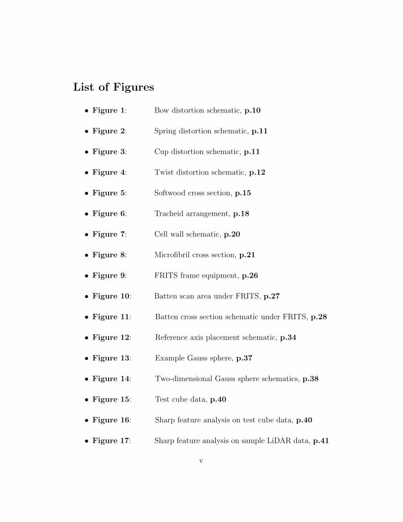
List of Figures
• Figure 1: Bow distortion schematic, p.10
• Figure 2: Spring distortion schematic, p.11
• Figure 3: Cup distortion schematic, p.11
• Figure 4: Twist distortion schematic, p.12
• Figure 5: Softwood cross section, p.15
• Figure 6: Tracheid arrangement, p.18
• Figure 7: Cell wall schematic, p.20
• Figure 8: Microfibril cross section, p.21
• Figure 9: FRITS frame equipment, p.26
• Figure 10: Batten scan area under FRITS, p.27
• Figure 11: Batten cross section schematic under FRITS, p.28
• Figure 12: Reference axis placement schematic, p.34
• Figure 13: Example Gauss sphere, p.37
• Figure 14: Two-dimensional Gauss sphere schematics, p.38
• Figure 15: Test cube data, p.40
• Figure 16: Sharp feature analysis on test cube data, p.40
• Figure 17: Sharp feature analysis on sample LiDAR data, p.41
v
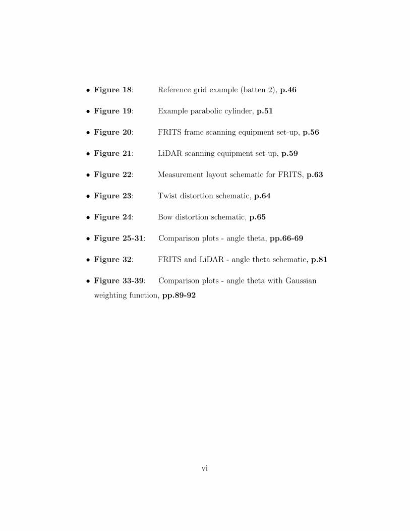
• Figure 18: Reference grid example (batten 2), p.46
• Figure 19: Example parabolic cylinder, p.51
• Figure 20: FRITS frame scanning equipment set-up, p.56
• Figure 21: LiDAR scanning equipment set-up, p.59
• Figure 22: Measurement layout schematic for FRITS, p.63
• Figure 23: Twist distortion schematic, p.64
• Figure 24: Bow distortion schematic, p.65
• Figure 25-31: Comparison plots - angle theta, pp.66-69
• Figure 32: FRITS and LiDAR - angle theta schematic, p.81
• Figure 33-39: Comparison plots - angle theta with Gaussian
weighting function, pp.89-92
vi
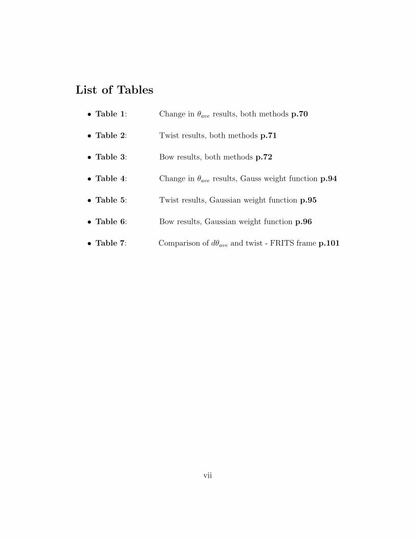
List of Tables
• Table 1: Change in θave results, both methods p.70
• Table 2: Twist results, both methods p.71
• Table 3: Bow results, both methods p.72
• Table 4: Change in θave results, Gauss weight function p.94
• Table 5: Twist results, Gaussian weight function p.95
• Table 6: Bow results, Gaussian weight function p.96
• Table 7: Comparison of dθave and twist - FRITS frame p.101
vii
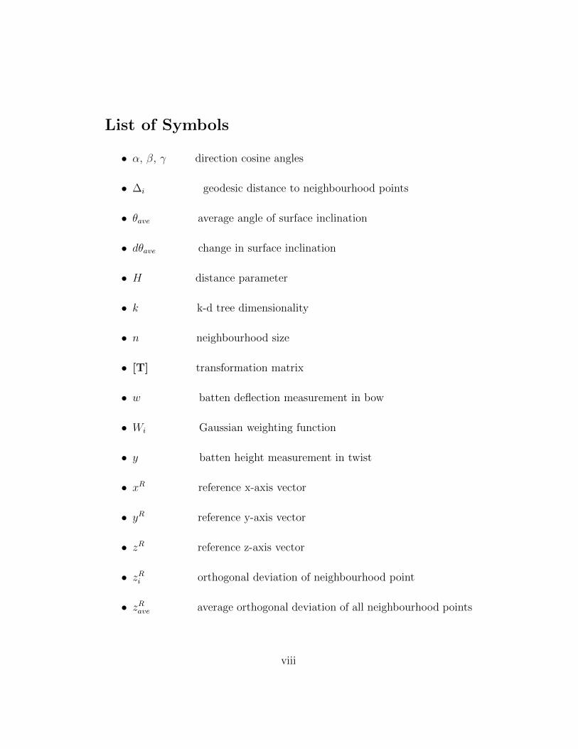
List of Symbols
• α, β, γ direction cosine angles
• ∆i geodesic distance to neighbourhood points
• θave average angle of surface inclination
• dθave change in surface inclination
• H distance parameter
• k k-d tree dimensionality
• n neighbourhood size
• [T] transformation matrix
• w batten deflection measurement in bow
• Wi Gaussian weighting function
• y batten height measurement in twist
• xR reference x-axis vector
• yR reference y-axis vector
• zR reference z-axis vector
• zRi orthogonal deviation of neighbourhood point
• zRave average orthogonal deviation of all neighbourhood points
viii
Contents
1 Introduction 5
1.1 Project Background . . . . . . . . . . . . . . . . . . . . . . . . 5
1.2 Grading and Classification Processes Within the Timber In-
dustry . . . . . . . . . . . . . . . . . . . . . . . . . . . . . . . 7
1.3 Feature Measurement Standards - BS EN 1310:1997 . . . . . . 9
2 Literature Review 14
2.1 Material Structure of Wood . . . . . . . . . . . . . . . . . . . 14
2.1.1 Macrostructure . . . . . . . . . . . . . . . . . . . . . . 14
2.1.2 Microstructure . . . . . . . . . . . . . . . . . . . . . . 17
2.1.3 Ultra-structure . . . . . . . . . . . . . . . . . . . . . . 19
2.1.4 Molecular Structure . . . . . . . . . . . . . . . . . . . . 20
2.2 Moisture in Wood . . . . . . . . . . . . . . . . . . . . . . . . . 22
2.2.1 Free Water . . . . . . . . . . . . . . . . . . . . . . . . 22
2.2.2 Bound Water . . . . . . . . . . . . . . . . . . . . . . . 22
2.2.3 Water Vapour . . . . . . . . . . . . . . . . . . . . . . . 23
2.2.4 Fibre Saturation Point . . . . . . . . . . . . . . . . . . 23
2.3 Summary . . . . . . . . . . . . . . . . . . . . . . . . . . . . . 23
3 FRITS Frame 26
3.1 Introduction . . . . . . . . . . . . . . . . . . . . . . . . . . . . 26
3.2 Feature Measurement with FRITS Frame - Surface Inclination 28
4 LiDAR Scanner 31
4.1 Introduction . . . . . . . . . . . . . . . . . . . . . . . . . . . . 31
1
4.2 LiDAR Technology . . . . . . . . . . . . . . . . . . . . . . . . 31
4.2.1 LiDAR Scanning - Measurement Method Overview . . 32
4.3 LiDAR Scanning Method Description . . . . . . . . . . . . . . 35
4.3.1 Reference Axis Placement . . . . . . . . . . . . . . . . 35
4.3.2 Sharp Feature Analysis Method . . . . . . . . . . . . . 35
4.3.3 Direct Vector Placement Method . . . . . . . . . . . . 42
4.3.4 Direction Cosine Angles & Transformation Matrix . . . 43
4.3.5 Point Translation & Reference Surface . . . . . . . . . 44
4.3.6 Reference Grid . . . . . . . . . . . . . . . . . . . . . . 45
4.3.7 k-Nearest Neighbour Search & Measurement Extraction 47
4.4 Alternative Approach To Feature Extraction from Point Cloud
Data Utilising Quadratic Surfaces . . . . . . . . . . . . . . . . 50
4.4.1 Quadratic Surfaces . . . . . . . . . . . . . . . . . . . . 50
4.4.2 Weighted Least Squares Approximation . . . . . . . . . 52
4.4.3 Canonical Form . . . . . . . . . . . . . . . . . . . . . . 53
5 Experiment Method Description 54
5.1 Introduction . . . . . . . . . . . . . . . . . . . . . . . . . . . . 54
5.2 FRITS Experiments . . . . . . . . . . . . . . . . . . . . . . . 54
5.3 LiDAR Experiments . . . . . . . . . . . . . . . . . . . . . . . 57
5.3.1 Comparison to FRITS Frame . . . . . . . . . . . . . . 60
6 Results 61
6.1 Introduction . . . . . . . . . . . . . . . . . . . . . . . . . . . . 61
6.2 Change in Surface Inclination Measurements . . . . . . . . . . 65
6.2.1 Average Theta Plots . . . . . . . . . . . . . . . . . . . 65
2
6.2.2 Change in Average Theta . . . . . . . . . . . . . . . . 70
6.3 Twist Measurements . . . . . . . . . . . . . . . . . . . . . . . 71
6.4 Bow Measurements . . . . . . . . . . . . . . . . . . . . . . . . 72
7 Comparative Analysis 73
7.1 Practical Aspects of Feature Measurement Experiments . . . . 73
7.1.1 FRITS Experiments . . . . . . . . . . . . . . . . . . . 73
7.1.2 LiDAR Experiments . . . . . . . . . . . . . . . . . . . 74
7.1.3 Measurement Errors . . . . . . . . . . . . . . . . . . . 77
7.2 Distortion Measurements . . . . . . . . . . . . . . . . . . . . . 79
7.2.1 Change in Surface Inclination . . . . . . . . . . . . . . 79
7.2.2 Twist . . . . . . . . . . . . . . . . . . . . . . . . . . . 82
7.2.3 Bow . . . . . . . . . . . . . . . . . . . . . . . . . . . . 84
7.2.4 Distortion Measurements Summary . . . . . . . . . . . 84
7.3 Weighted Averaging Method - Comparison with Gaussian Weight-
ing Function . . . . . . . . . . . . . . . . . . . . . . . . . . . . 87
7.3.1 Change in Surface Inclination with Gaussian Weight-
ing Function . . . . . . . . . . . . . . . . . . . . . . . . 89
7.3.2 Twist Measurements with Gaussian Weighting Function 95
7.3.3 Bow Measurements with Gaussian Weighting Function 96
7.3.4 Summary . . . . . . . . . . . . . . . . . . . . . . . . . 97
8 Discussion 100
8.1 Existing Standards . . . . . . . . . . . . . . . . . . . . . . . . 100
8.2 Outlook for the Use of LiDAR Scanning Within Timber Research102
9 Conclusion 106
3

10 References 108
4
Investigating the use of LiDAR scanning as a
method for the measurement of timber
distortion features
September 4, 2016
1 Introduction
1.1 Project Background
Macroscopic distortion of structural-grade timber is a source of considerable
concern within the timber industry. As a piece of timber is dried its shape
can become greatly altered, potentially rendering it unsuitable for use as a
structural element. This alteration of shape, and the subsequent rejection of
structural timber not fit for final use, generates waste within the industry,
both material and financial.
Within the wider field of timber research, much focus has centred on under-
standing the mechanisms that drive distortion: namely, the material profile
5
of wood itself (including its moisture content) and the environmental con-
ditions to which the wood is subjected. However, in order to describe how
distortion develops, measuring distortion in a meaningful and universal way
is an important first step. Accurately describing the shape (and therefore the
potential usability) of a timber batten provides a key function to ensuring
efficiency within timber selection procedures.
For relatively small scale experiments, the FRITS frame method is currently
the established approach in measuring the surface profile of structural tim-
ber pieces. Typically, this method relies on a large degree of interpolation
between relatively few measurement points across the timber surface to de-
scribe its overall shape. It is the purpose of this project to investigate the
use of LiDAR scanning as an alternative approach to measuring distortion
features of timber.
The considerably greater number of measurement points taken by the LiDAR
scanner generates a more comprehensive description of the timber macro-
scopic profile. In taking measurements across the entire surface area the
need for highly interpolative measuring is markedly reduced. Further, LiDAR
scanning in this context is considerably quicker than current approaches, with
set-up and scan time far shorter than FRITS. The method also allows for
measurements to be taken in any environment, the LiDAR scanner being a
highly transportable piece of equipment.
LiDAR scanning is a well-established measurement tool in many other fields
6
and allows for detailed scans to be taken in a variety of environments. This,
coupled with the quickness and efficiency of the technology warrants explo-
ration into its applicability within timber distortion measurement.
1.2 Grading and Classification Processes Within the
Timber Industry
Strength grading of structural timber consists of visual and machine grading
where timber is classified based on assessment of its strength, stiffness and
density. Within machine grading, a process of visual override is undertaken
to manually reject timber samples that fail a visual inspection. Here, vi-
sual override concerns a range of macroscopic features that may influence a
piece of timber’s structural performance. Obvious signs of obliquity within
the sawn timber’s profile, in addition to the presence and concentration of
macroscopic defects (such as knots and fissures, rot and insect damage), will
help determine a batten’s final grading [BS EN 14081-1, 2016]. Typ-
ically, the process of visual override is slow in comparison to mechanised
solutions and requires third party certification. By necessity, the gradings
given through visual inspections are conservative [Holland and Reynolds,
2005].
For detailed assessments, machine grading is used to determine the quality
of a given piece of structural timber. Machine grading techniques for struc-
tural timber allow for non-destructive assessment of structural performance.
Previously, three-point bending equipment was a standard method for non-
destructive measurements. More recently, however, three-point bending ma-
7
chines are being replaced by x-ray scanning and acoustic resonance testing.
With X-ray and microwave scanning, it is possible to measure the presence
of knots and the slope of the grain: properties relevant not only to quality
control but also structural performance and strength grading [Goldeneye,
2016]. Laser interferometer scanners can measure resonance frequency of a
timber board, enabling accurate, reliable calculation of the timber’s modulus
of elasticity [Viscan, 2016]. Moisture profiles within the wood material
can also be studied using Computed Tomography (CT) scanners [Sandberg
and Salin, 2012].
Concerning surface-related characteristics of timber, laser-based surface scan-
ning techniques allow for precise dimensional measuring of logs and sawn
timber pieces, helping to ensure efficient, economic output from the sawmill.
A range of commercial scanning equipment exists which can rapidly generate
360◦ imaging of a piece of timber, including the end surfaces. Output from
these detailed scans allows for measurement of annual growth rings, slope of
the grain and the position of the pith: key measurements within quality con-
trol procedures [WoodEye, 2016]. High-end laser-based scanning solutions
also exist to provide precise measurement of distorted boards [Curvescan,
2016]. These solutions rely on laser triangulation processes, as opposed to
LiDAR devices which rely on a time-of-flight approach.
In smaller, bench-top environments analogue means are generally employed
to measure macroscopic features. Scaled devices for measurement of bow,
spring, cup and twist (see section 1.3) allow for reliable measurements with
8
minimal expense [Grohmann et al., 2010].
The investigations of this thesis focus on the potential to develop a middle
path in distortion measurement. The use of large-scale scanning equipment
within the timber industry provides saw mills with a highly innovative and
ever expanding approach to timber grading. However, the scale and ex-
pense of such machinery currently prohibits their widespread use in humbler
settings, particularly within a research environment. While bench-top tech-
niques using hand-held analogue tools allow for an accessible and inexpensive
alternative to distortion measurement, the information gleaned in this way is
limited, lacks standardisation, and fails to provide the greater level of detail
afforded by industrialised scanning techniques.
As such, an intermediate approach that exploits the detailed measuring ca-
pabilities of scanning methods while remaining accessible and practical for
small scale testing environments would be a worthwhile addition to the tim-
ber research community.
1.3 Feature Measurement Standards - BS EN 1310:1997
Using existing standards for feature measurement of timber, information can
be extracted from measurement data sets (be they from FRITS or LiDAR
scanning) to assess the distortion of each batten. The current guidelines
provide a standard by which to compare output from the existing FRITS
method with output from the alternative LiDAR method.
9
Existing European guidelines on feature measurement of round and sawn
timber are contained within BS EN 1310:1997. These list four types of dis-
tortion in timber battens: bow, spring, cup and twist. In order for a timber
batten to be used successfully as a structural component, the degree to which
it has distorted is important. Battens with little or no deviations from a flat,
orthogonal shape respond more consistently to external loads, producing a
more reliable structural performance than highly deviated battens. Distorted
battens can produce difficulties on a construction site in fitting together tim-
ber kits and can eventually cause defects in the finished construction, such
as squeaking doors and uneven floors. As such, measuring how a batten
deviates from an undeformed shape on a macro level provides a partial yet
useful insight into a batten’s structural integrity and its potential use as a
structural, load-bearing member. Figures 1 to 4 depict the characteristics
of each distortion type as well as the criteria by which they are measured
[British Standards Institute, 1997].
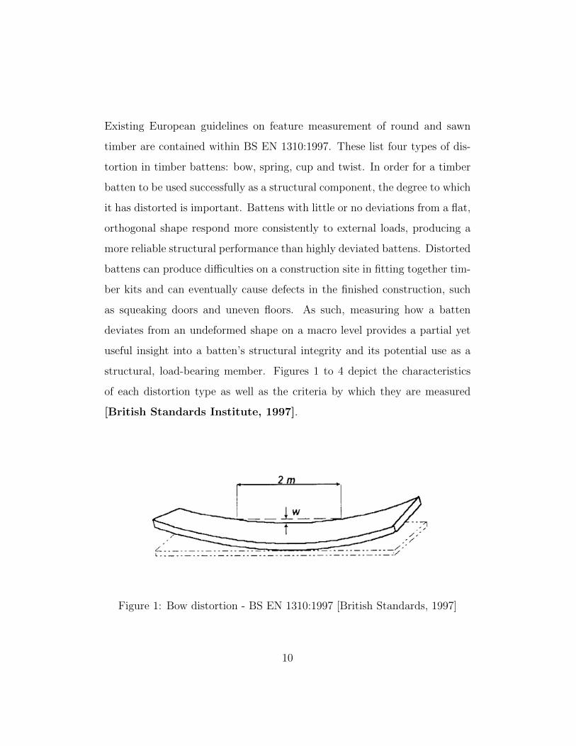
Figure 1: Bow distortion - BS EN 1310:1997 [British Standards, 1997]
10
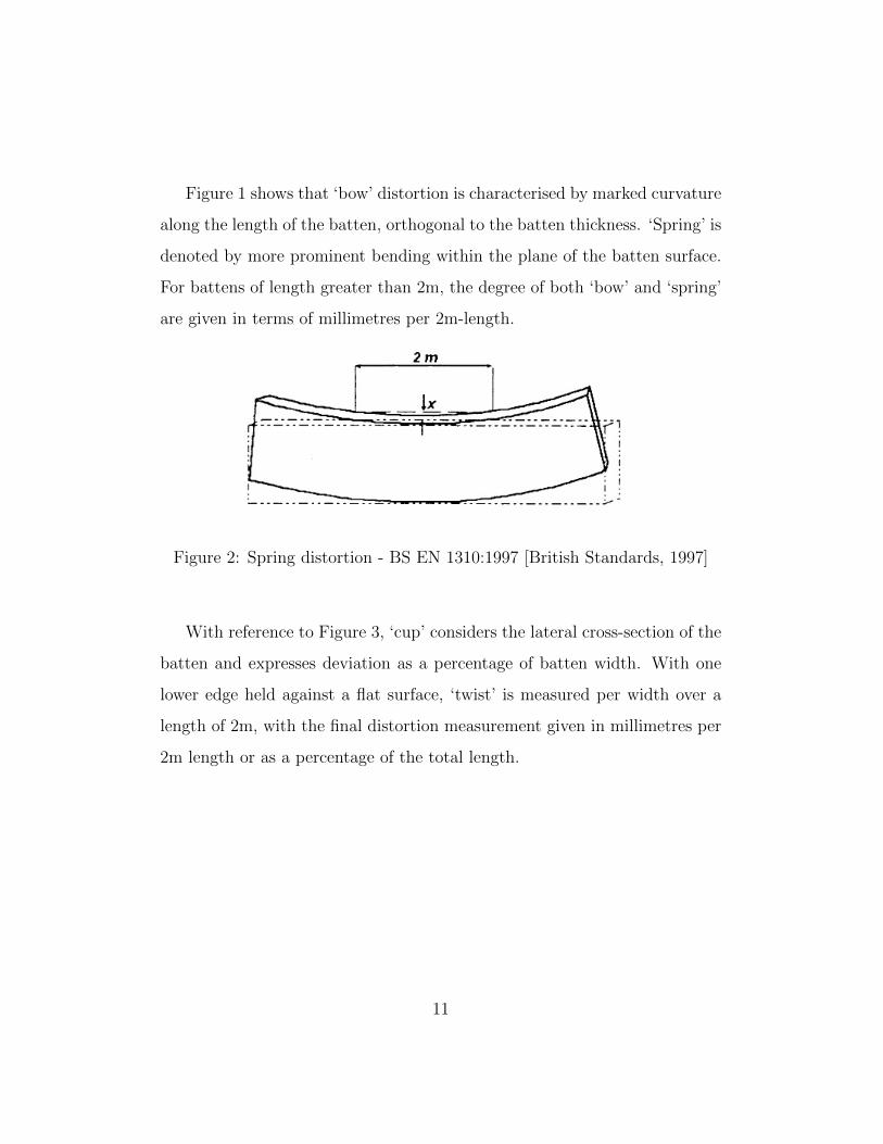
Figure 1 shows that ‘bow’ distortion is characterised by marked curvature
along the length of the batten, orthogonal to the batten thickness. ‘Spring’ is
denoted by more prominent bending within the plane of the batten surface.
For battens of length greater than 2m, the degree of both ‘bow’ and ‘spring’
are given in terms of millimetres per 2m-length.
Figure 2: Spring distortion - BS EN 1310:1997 [British Standards, 1997]
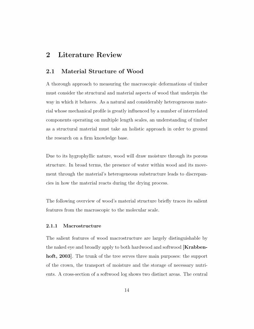
With reference to Figure 3, ‘cup’ considers the lateral cross-section of the
batten and expresses deviation as a percentage of batten width. With one
lower edge held against a flat surface, ‘twist’ is measured per width over a
length of 2m, with the final distortion measurement given in millimetres per
2m length or as a percentage of the total length.
11
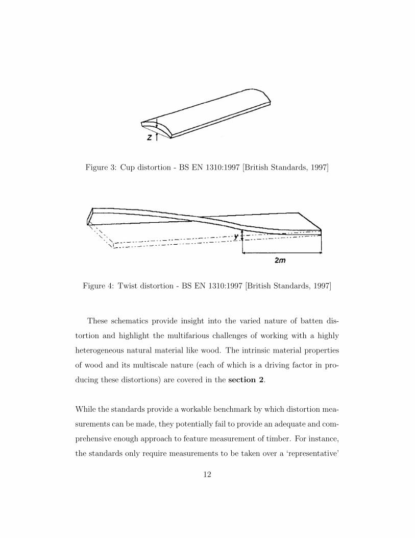
Figure 3: Cup distortion - BS EN 1310:1997 [British Standards, 1997]
Figure 4: Twist distortion - BS EN 1310:1997 [British Standards, 1997]
These schematics provide insight into the varied nature of batten dis-
tortion and highlight the multifarious challenges of working with a highly
heterogeneous natural material like wood. The intrinsic material properties
of wood and its multiscale nature (each of which is a driving factor in pro-
ducing these distortions) are covered in the section 2.
While the standards provide a workable benchmark by which distortion mea-
surements can be made, they potentially fail to provide an adequate and com-
prehensive enough approach to feature measurement of timber. For instance,
the standards only require measurements to be taken over a ‘representative’
12

2m length as described above, providing no specifications as to what ‘rep-
resentative’ may mean for battens of various lengths. Further, limiting the
number of distortion features by which a batten can be described to just four
may not be exhaustive enough to meet the highly varied nature of timber
distortion. These doubts regarding the efficacy and completeness of the stan-
dards in part motivate the research carried out here.
Nevertheless, in this project the standards given in BS EN 1310:1997 will
serve as a useful reference from which distortion features can be measured.
This will allow for standardised comparisons between the existing FRITS
technique and the LiDAR approach proposed here, helping validate the ac-
curacy of the new method.
13
2 Literature Review
2.1 Material Structure of Wood
A thorough approach to measuring the macroscopic deformations of timber
must consider the structural and material aspects of wood that underpin the
way in which it behaves. As a natural and considerably heterogeneous mate-
rial whose mechanical profile is greatly influenced by a number of interrelated
components operating on multiple length scales, an understanding of timber
as a structural material must take an holistic approach in order to ground
the research on a firm knowledge base.
Due to its hygrophyllic nature, wood will draw moisture through its porous
structure. In broad terms, the presence of water within wood and its move-
ment through the material’s heterogeneous substructure leads to discrepan-
cies in how the material reacts during the drying process.
The following overview of wood’s material structure briefly traces its salient
features from the macroscopic to the molecular scale.
2.1.1 Macrostructure
The salient features of wood macrostructure are largely distinguishable by
the naked eye and broadly apply to both hardwood and softwood [Krabben-
hoft, 2003]. The trunk of the tree serves three main purposes: the support
of the crown, the transport of moisture and the storage of necessary nutri-
ents. A cross-section of a softwood log shows two distinct areas. The central
14
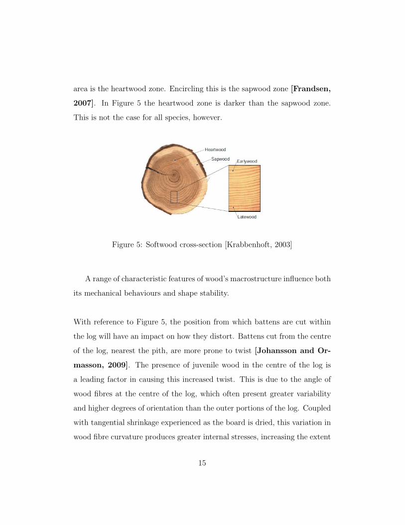
area is the heartwood zone. Encircling this is the sapwood zone [Frandsen,
2007]. In Figure 5 the heartwood zone is darker than the sapwood zone.
This is not the case for all species, however.
Figure 5: Softwood cross-section [Krabbenhoft, 2003]
A range of characteristic features of wood’s macrostructure influence both
its mechanical behaviours and shape stability.
With reference to Figure 5, the position from which battens are cut within
the log will have an impact on how they distort. Battens cut from the centre
of the log, nearest the pith, are more prone to twist [Johansson and Or-
masson, 2009]. The presence of juvenile wood in the centre of the log is
a leading factor in causing this increased twist. This is due to the angle of
wood fibres at the centre of the log, which often present greater variability
and higher degrees of orientation than the outer portions of the log. Coupled
with tangential shrinkage experienced as the board is dried, this variation in
wood fibre curvature produces greater internal stresses, increasing the extent
15

to which the wood distorts at a macro level [Johansson and Ormasson,
2009; Sandberg, 2005]. To this end, strategic cutting procedures are re-
quired within sawmills to ensure structural timber is cut furthest from the
pith.
The way in which a tree grows can greatly influence the material compo-
sition (and subsequent mechanical properties) of the timber it yields. Where
a tree grows at an orientation or out of equilibrium, reaction wood develops.
Reaction wood can be formed by a number of environmental factors, from
wind exposure, snow loadings, sloping ground and asymmetries within the
tree shape. While the chemical and material changes unique to reaction wood
are a necessary adaptation that allows the continued growth of the tree, the
timber it yields demonstrates poor mechanical performance [Du and Ya-
mamoto, 2007]. In softwoods, where wood material has been subjected
to compressive forces (for example, on the underside of a sloping tree or on
the leeward side of a tree exposed to strong winds) compression wood forms.
Variations within the material profile of compression wood, in particular a
higher microfibril angle (see section 2.1.2), can greatly impact the wood’s
future shape stability [Forestry Commission, 2003].
Mechanical behaviour of the timber can also be influenced by knots within
the wood surface [Lukacevic et al., 2014]. Localised distortions of the
grain direction are created around the knot, leading to disturbances in stress
distributions. The resultant sloping grain around knots can reduce tension
strength, compromising a batten’s potential structural performance [New
16
Zealand Timber Industry Federation, 2007].
Of further consideration to macroscopic distortion is the influence of the
drying process. How the battens are dried and the way in which they are
stored and restrained throughout can have an influence on their final mor-
phology [Johansson, 2006]. This shows clearly how early on in the milling
process a batten’s future shape stability can be determined.
2.1.2 Microstructure
On a cellular level, the microstructure of wood comprises an arrangement
of longitudinal, approximately square cells known as tracheids. These cells
do not follow exactly the direction of the longitudinal axis of the tree, but
instead present a spiral or helical orientation, similar to the orientations
of the wood grain. This spiral grain angle varies within the stem and is
typically no more than 5◦ [Neagu et al., 2006]. Newly formed tracheid
cells serve to transport water throughout the tree. Their large cross-section
and thin cell walls allow this. As the tree grows, new tracheid cells form to
provide structural support. Here, developing tracheid cells display smaller
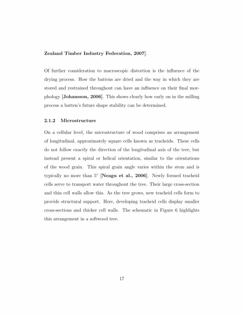
cross-sections and thicker cell walls. The schematic in Figure 6 highlights
this arrangement in a softwood tree.
17
Figure 6: Tracheid arrangment [Krabbenhoft, 2003]
The development of these tracheid cells as the tree grows can have a
significant impact on macroscopic distortion. Longitudinal compression of
cells creates internal stresses within the wood, as compressed cells pull on
adjoining cells. The distribution of these internal stresses will affect how
the batten distorts after sawing [Johansson and Ormasson, 2009]. The
movement of moisture through the cell structure, particularly during the dry-
ing process, is also a key factor in generating distortion [Fransden, 2007].
Further, the angle of spiral grain contributes significantly to macroscopic dis-
tortions. Larger values of spiral grain angle have shown a strong correlation
with greater degrees of shape instability, particularly towards the develop-
ment of twist [Watt et al., 2013, Ekevad, 2005].
18
2.1.3 Ultra-structure
The cell wall of each tracheid comprises a multi-layered structure consisting
of a primary wall (P) and a secondary wall (S ). This secondary wall is in
itself comprised of a number of layers: S1 = outer layer, S2 = middle layer
and S3 = inner layer. These are shown in Figure 7. Though the layers differ
in terms of thickness and composition, each is constructed from a matrix
material reinforced by microfibrils.
Packed tightly together, these thread-like microfibrils constitute the material
structure of the cell wall, with each microfibril measuring around 5000nm in
length and between 10 and 20nm in width [Krabbenhoft, 2003].
The discrepancies between microfibril orientations within the secondary wall
provide much of the structural rigidity of the cell wall. The release of internal
stresses when the batten is cut from the log plays a key role in generating
macroscopic distortion. The readjustment of fibres at this ultrascale, cou-
pled with the movement of moisture through the network of lumens, greatly
determines the batten‘s final shape.
19
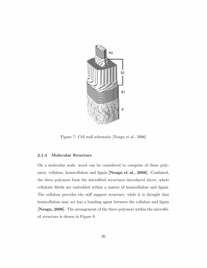
Figure 7: Cell wall schematic [Neagu et al., 2006]
2.1.4 Molecular Structure
On a molecular scale, wood can be considered to comprise of three poly-
mers: cellulose, hemicellulose and lignin [Neagu et al., 2006]. Combined,
the three polymers form the microfibril structures introduced above, where
cellulosic fibrils are embedded within a matrix of hemicellulose and lignin.
The cellulose provides the stiff support structure, while it is thought that
hemicellulose may act has a bonding agent between the cellulose and lignin
[Neagu, 2006]. The arrangement of the three polymers within the microfib-
ril structure is shown in Figure 8.
20
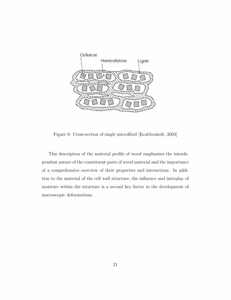
Figure 8: Cross-section of single microfibril [Krabbenhoft, 2003]
This description of the material profile of wood emphasises the interde-
pendent nature of the constituent parts of wood material and the importance
of a comprehensive overview of their properties and interactions. In addi-
tion to the material of the cell wall structure, the influence and interplay of
moisture within the structure is a second key factor in the development of
macroscopic deformations.
21
2.2 Moisture in Wood
As with the material structure of wood, an accurate description of water
in wood requires analysis on a number of different levels. In this instance,
‘moisture’ does not simply mean liquid water. Rather, it encompasses three
distinct forms. Here, moisture states are discussed within the context of
green timber drying.
2.2.1 Free Water
Typically, free water is found only in living trees and wood in direct contact to
water. There is an upper limit to the amount of moisture the fibrous cell wall
material can hold. When this limit is exceeded, free water is formed which is
then transported through void spaces within the tracheids [Krabbenhoft,
2003]. The influence of free water on macroscale mechanical properties of
wood is negligible [Eitelberger, 2011].
2.2.2 Bound Water
In this form, water molecules which are chemically bonded by intermolecular
forces to the wood substance are considered. Linked to fluctuations in relative
humidity, changes in bound water concentration bring about volume changes
in the cell wall. It is the associated strains and stresses which thus lead to
shrinkages and swelling in the macrostructure of the wood [Eitelberger,
2011].
22
2.2.3 Water Vapour
As liquid water begins to dry, it is replaced by a mixture of air and wa-
ter vapour. This water vapour is particularly difficult to model accurately
[Krabbenhoft, 2003].
2.2.4 Fibre Saturation Point
The concept of a fibre saturation point becomes pertinent to the discussion of
macro-level distortion when we consider that macroscopic deformations only
occur at moisture content levels below the FSP. With battens routinely kiln
dried to moisture contents of around 18%, the conditions under which defor-
mations are likely to occur will almost certainly be met in most commercial
drying processes. Drying freshly cut, green-state timber battens from rela-
tively high moisture content levels to moisture contents sufficiently below the
FSP instigates moisture transport mechanisms which create movement and
shrinkage across the cell wall material, in turn driving macroscopic changes
to the timber batten shape.
Again, by assessing the state and influence of moisture in timber, another
layer of interconnectivity is added to the hierarchical nature of wood’s ma-
terial behaviour.
2.3 Summary
As part of an investigation into macroscale distortion measurement, the de-
scription of wood as a mutliscale, hygrophyllic and extremely heterogeneous
23
material presented here is vital to understanding the influencing factors that
drive distortion to begin with.
The shape of a distorted timber batten as observed at the macroscale is
the result of complex interactions within the wood material across multiple
length scales. In addition, the presence and movement of moisture through
the wood material will greatly determine the batten’s final form.
Wood as a structural material obtains its stiffness from the rigid, densely
packed structure of its cell walls. The rigidity of the cell wall is achieved by
stiff microfibrils, wrapped in contrasting helical patterns in a number of lay-
ers to form the cell wall structure. These microfibrils act together to resist
axial and torsional movements. The stiffness of the microfibrils is in turn
gained from its matrix composition of polymers: cellulose, hemicellulose and
lignin. Cellulose provides much of the structural support to this matrix; how-
ever, the interplay between all three polymers ensures support is provided in
longitudinal and transverse directions. Upon cutting the timber, the internal
stresses of the microfibrils- rooted at the molecular scale- experience a release
and begin to pull the cell wall material.
Further, as the timber is dried, a movement of moisture is instigated through
the network of lumens within the cell wall as moisture travels from levels of
high concentration to low. The anisotropic nature of wood ensures that mois-
ture distribution and movement is not constant across the material. Thus
moisture level gradients are created. The presence of moisture in the cell
24
wall structure (either as bound water or water vapour) causes swelling and
shrinkage of the cell wall material. The uneven distribution of moisture will
naturally lead to uneven shrinkages and swelling across the cell wall network.
These molecular level movements and interactions eventually scale up, through
the material structure described above, to generate movements at the macro
level. It is these macroscopic movements that are of interest to this thesis.
However, as we have shown, their origin is of a much smaller, more subtle
dimension.
Presenting a new method for measuring timber distortion, as is the pur-
pose of this thesis, without consideration to its fundamental causes would
leave the work detached from the wider context in which it sits. A macro-
scopic description of timber distortion features addresses how a batten has
deformed and to what extent. However, a multiscale understanding of the
nature of wood and its properties addresses why the batten presents such
deformations.
25
3 FRITS Frame
3.1 Introduction
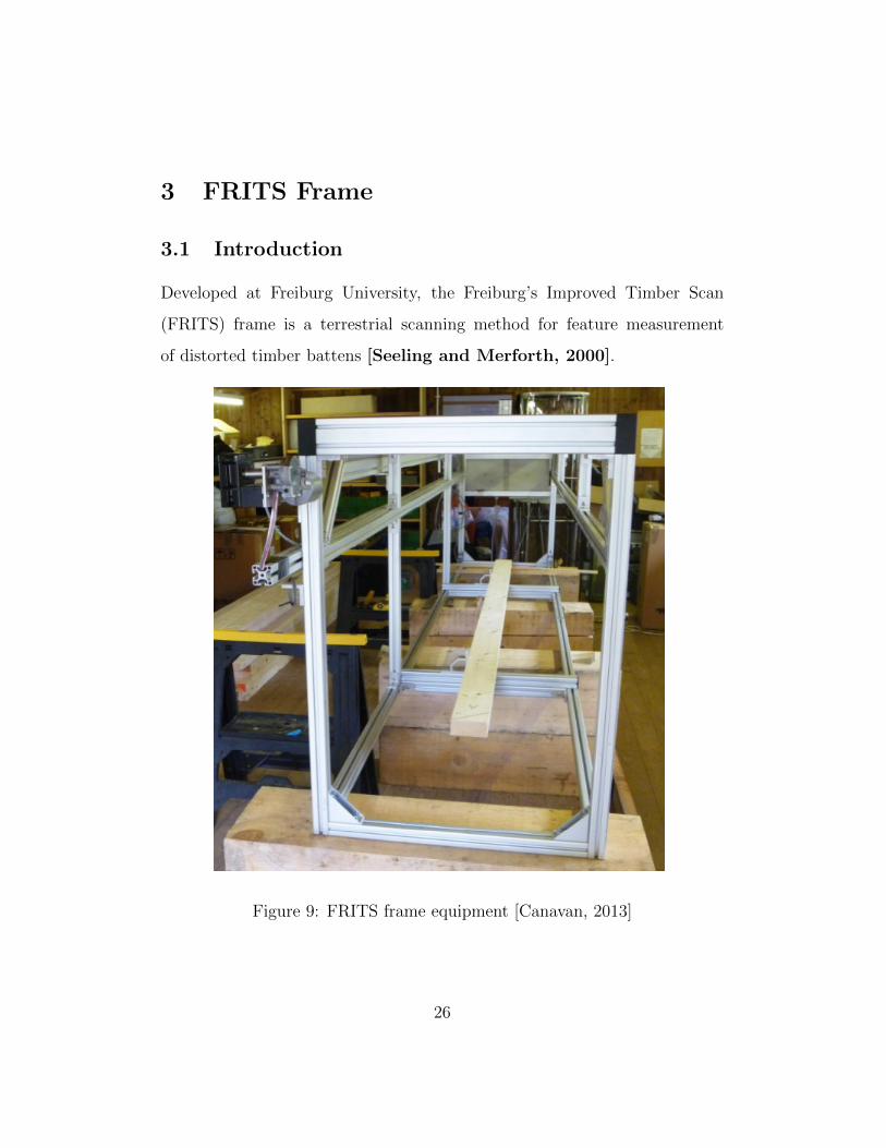
Developed at Freiburg University, the Freiburg’s Improved Timber Scan
(FRITS) frame is a terrestrial scanning method for feature measurement
of distorted timber battens [Seeling and Merforth, 2000].
Figure 9: FRITS frame equipment [Canavan, 2013]
26

A ‘semi-automated’ method, the FRITS frame comprises a steel frame
structure, in which the batten sits, and a set of two lasers. Distortion is
measured by one laser measuring vertical displacement at prescribed intervals
along the length of the batten, the longitudinal position being logged by the
horizontal laser.
Figure 10: Scan area of batten surface under FRITS frame scanning
Figure 10 shows a typical scan layout for a batten in the FRITS method.
A measurement is taken at each intersection point of the scan grid. Note
that the scan area does not cover the entirety of the batten surface and that
the number of measurements taken is relatively small.
27
3.2 Feature Measurement with FRITS Frame - Surface
Inclination
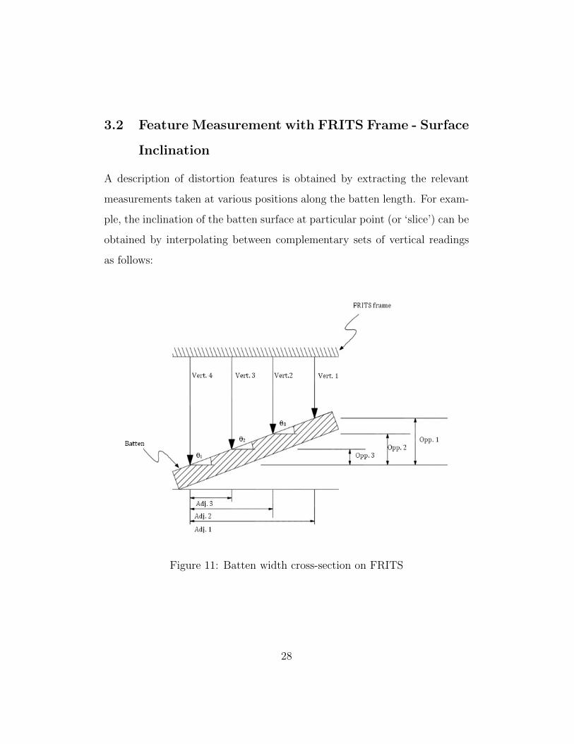
A description of distortion features is obtained by extracting the relevant
measurements taken at various positions along the batten length. For exam-
ple, the inclination of the batten surface at particular point (or ‘slice’) can be
obtained by interpolating between complementary sets of vertical readings
as follows:
Figure 11: Batten width cross-section on FRITS
28

Opp.1 = V ert.4− V ert.1 (1)
Opp.2 = V ert.4− V ert.2 (2)
Opp.3 = V ert.4− V ert.3 (3)
Each of the ‘Vert.’ displacements represents a measurement taken by the
vertical laser along the length of the batten. The adjacent values (Adj.|1,2,3)
are measured manually. The position of these measurements is at the dis-
cretion of the user, depending on the size of the scan area and the number
of measurement points desired. For a standard 3m long batten of width
100mm, three adjacent lengths of approximately 20mm, measured 20mm in
from the batten edge provide a suitably wide scan area, while ensuring all
points remain on the batten surface.
From Figure 11, each ‘slice’ taken with the FRITS frame contains three an-
gles, θ|1,2,3. A linear interpolation is used to calculate an angle of inclination
for the ‘slice’. Given the relatively short distance between measurements,
describing the batten surface by three separate linear interpolations and av-
eraging the results provides a good approximation for the change in surface
inclinations. A detailed description of the experiment set-up is given in sec-
tion 5.2.
29
θ1 = tan−1(Opp.1
Adj.1) (4)
θ2 = tan−1(Opp.2
Adj.2) (5)
θ3 = tan−1(Opp.3
Adj.3) (6)
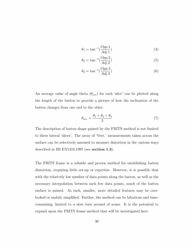
An average value of angle theta (θave) for each ‘slice’ can be plotted along
the length of the batten to provide a picture of how the inclination of the
batten changes from one end to the other.
θave =θ1 + θ2 + θ3
3(7)
The description of batten shape gained by the FRITS method is not limited
to these lateral ‘slices’. The array of ‘Vert.’ measurements taken across the
surface can be selectively assessed to measure distortion in the various ways
described in BS EN1310:1997 (see section 1.3).
The FRITS frame is a reliable and proven method for establishing batten
distortion, requiring little set-up or expertise. However, it is possible that
with the relatively low number of data points along the batten, as well as the
necessary interpolation between such few data points, much of the batten
surface is missed. As such, smaller, more detailed features may be over-
looked or unduly simplified. Further, the method can be laborious and time-
consuming, limited to a slow turn around of scans. It is the potential to
expand upon the FRITS frame method that will be investigated here.
30
4 LiDAR Scanner
4.1 Introduction
In this section the nature of LiDAR technology is discussed before introduc-
ing a method for using LiDAR scanning to describe the distortion of timber
battens. Investigation was undertaken to determine how this new method
performs as a practical, reliable alternative measurement technique. Pro-
viding a more detailed description of the batten surface, in contrast to the
point-wise analysis of the FRITS frame, the use of LiDAR scanning was
investigated as an alternative methodology in macroscopic feature analysis.
4.2 LiDAR Technology
Light Detection and Ranging (LiDAR) technology has been used extensively
in a number of fields to provide accurate three-dimensional depictions of
objects and environments. A standard tool in architectural studies, land
surveying and mapping, the technology has seen an increase in its demand
and popularity over the last ten years [Sun and Salvaggio, 2013]. While
technical details may differ from model to model, a LiDAR scanner collects
information about its spatial environment by rotating around a fixed point,
emitting intermittent beams of light (be it ultra-violet, visible or infra-red)
onto surrounding surfaces. The reflected beams of light are processed and
31
a three-dimensional polar coordinate of each reflected point is stored. The
resulting data set, known as a point cloud, comprises a list of these coordi-
nates with no reference to their connectivity or their relationship with one
another. The only raw measurement gleaned from the LiDAR scan is the
distance from the scanner to the surface off which the laser reflects. It falls
to the user as to what post-processing is carried out on the point cloud, de-
pending on the focus of the research or application. This open-ended nature
of how scans can be used is very much a key motivator in investigating and
validating the use of LiDAR scans in timber research.
Point cloud data returned from these scans benefits from a high level of
detail and accuracy, with the resultant images providing a faithful repre-
sentation of the scan environment. The versatility of scanning equipment,
coupled with developments in both scan technology and the software used in
post-processing has guided this research into exploring a new, fertile area of
inquiry for the timber industry.
4.2.1 LiDAR Scanning - Measurement Method Overview
The method proposed here for distortion measurement aims to utilise the ex-
tensive detail gained from the LiDAR scan to describe the distorted surface
and compare its performance to more conventional methods.
In essence, the LiDAR scanning method describes a batten surface using
the same concept as the FRITS frame method, only with a far greater, more
extensive number of sample points. With the FRITS frame, vertical devia-
32
tion is measured from a fixed datum at selected points across the batten. In
each FRITS scan, the datum is set by the frame structure in which the bat-
ten sits. In the LiDAR method here, however, the only piece of information
obtained from the point cloud is the global coordinates of each of the points.
Their connectivity and the shape they describe are unknown at the outset.
As such, the first key challenge in this method is to construct a standardised
datum for each scan. This datum is called the reference surface and it serves
as a benchmark from which distortion measurements are made with LiDAR
scanning.
The reference surface is a flat plane described by its own reference coor-
dinate system (xR, yR, zR), independent of the global coordinate system
(x,y, z) established by the LiDAR scanner (the scanner itself acts as origin
to the global scheme). As shown in Figure 12 below, the reference axes (xR,
yR) are positioned such that their origin is positioned approximately at a
batten corner edge, with the xR axis approximately aligning with the short
edge of the batten; the yR axis following the general direction of the long
edge. The vectors describing the reference axes are necessarily orthogonal
to each other. The reference axes could be positioned anywhere in space;
however, this placement convention was the simplest choice.
33

Figure 12: Reference axis placement
By using a transformation matrix consisting of the direction cosines of the
reference axis vectors, global coordinates of the point cloud data (x,y, z) are
rotated into equivalent reference coordinates (xR, yR, zR). The reference xR
& yR values describe the position of each LiDAR point projected onto the
reference surface. The reference zR value describes the orthogonal deviation
of that point to the reference surface: equivalent to the deviation measured
by the FRITS.
Following the approximate shape described by the projected points on the
reference surface, a grid network, called the reference grid, is established.
Each point on the reference grid uses the orthogonal deviations of the near-
34

est surrounding points on the reference surface to establish an averaged or-
thogonal deviation value. Thus, each point on the reference grid provides an
approximated description of how the batten surface sits in space. It is to the
discretion of the user which distortion features are extracted from this data.
4.3 LiDAR Scanning Method Description
4.3.1 Reference Axis Placement
The Cartesian coordinates obtained from LiDAR scans are the only raw data
needed to calculate distortion in this method. In order to transform the Li-
DAR points onto a reference surface, a separate coordinate system must be
created, distinct from the x,y,z-axes of the LiDAR scanner. Those edges rep-
resenting the width and length of the batten are used to position the xR and
yR-axes respectively, ensuring that neither axis deviates too greatly from the
batten edge while maintaining their necessary orthogonal relationship (This
reduces the need for extra spatial translations when projecting points onto
the surface). A third axis zR is calculated from the cross product of xR and
yR. These three vectors are then used to construct a transformation matrix,
converting raw LiDAR coordinates into the equivalent reference coordinates.
4.3.2 Sharp Feature Analysis Method
In the initial stages of this investigation, an almost automatic approach to es-
tablishing the xR and yR axes was sought, whereby the reference axes would
be created and positioned directly from the raw point cloud data without
requiring any initial assessment or calculation. This approach sought to use
35
existing methods of feature extraction from point cloud data sets, specifically
the detection method of ‘sharp’ features as described by Weber, Hahmann
et al [2010].
In their approach, information about the position of each point in the cloud
is obtained by analysing a ‘neighbourhood’ of its surrounding points. How
the cross-products of consecutive pairs of neighbourhood points vary in their
directions provides insight into whether the point under analysis is ‘sharp’
or ‘flat’, with sharp and flat points showing marked differences in the way
in which cross products are distributed. This type of analysis, described in
detail below, would allow one to identify the batten edges within the point
cloud and place the reference axes along their appropriate edges as required.
By this method, a k-nearest neighbourhood search is carried out across the
point cloud set. This type of classification algorithm uses the surrounding
data set to categorize a particular point based on the nearest surrounding
points within the data set. Using the Euclidean distances between the point
in question and the surrounding set, the point is classified based on a major-
ity of the k-nearest points.
For the model presented here, the point cloud functions as the data set.
Each point in the point cloud is considered in turn. Based on its coordi-
nates, open source neighbourhood search tools (described in detail in sec-
tion 4.3.7) establish which of the surrounding points are nearest according
to their geodesic distances. Given a chosen value for ‘k’, the neighbourhood
36
search selects the k-nearest points and stores them as a vector. This vector
is known as the point’s neighbourhood.
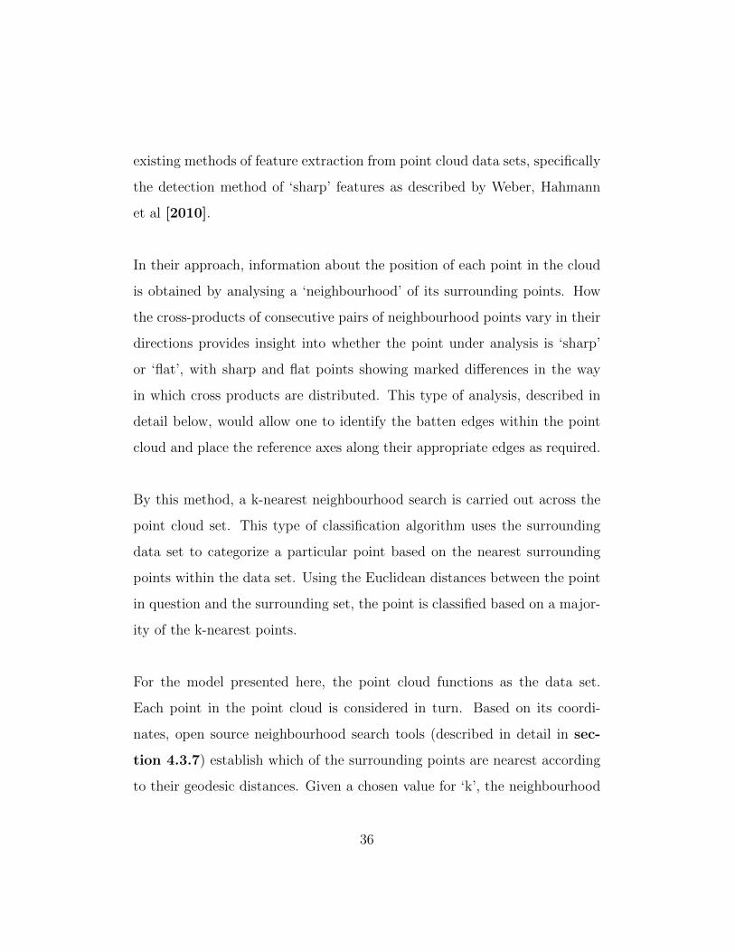
Each neighbourhood is then considered in turn. Within a neighbourhood, a
unit Gauss sphere is created, centred on the point under analysis. A unit
Gauss sphere translates the unit normal vector of a point on a surface onto
its equivalent position on unit sphere surface. Within these Gauss spheres,
sequential pairs of cross products are calculated using the surrounding neigh-
bourhood points. These cross products are projected up onto the unit Gauss
sphere surface where their clustering patterns can be analysed.
Figure 13: Gauss sphere example [Weber, Hahmann et al, 2010]
In Figure 13, the red point in the centre of the Gauss sphere is the point
under analysis. The yellow points are its neighbouring points, i.e. points
that are closest to the red point (In this example neighbourhood size, k =
12). The black points fall outwith the neighbourhood and are not included
in the calculations.
37
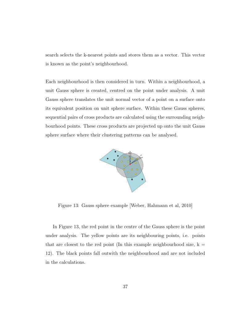
Depending on where the point under analysis is positioned on the batten sur-
face, the cross products projected onto the Gauss sphere will be distributed
in a number of ways. As such, the standard deviation of these distances
will markedly change depending on the distribution. The two-dimensional
Gauss sphere schematics in Figure 14 highlight three examples of how cross
products may be spread on the unit sphere surface.
Figure 14: Two-dimensional Gauss sphere schematics; left-right: flat surface,
high curvature, sharp feature [Weber, Hahmann et al, 2010]
With reference to Figure 14, the first case shows a point comfortably po-
sitioned on a flat surface. All the points within its neighbourhood lie on the
same plane, thus the cross products created all point in the same direction
and present a notably concise cluster on the Gauss sphere. As a result of
this, the standard deviation of geodesic distances between these points on
the Gauss sphere will be low.
The second schematic describes the distribution of a point on an area of
high curvature. This particular feature would not be present in scanning
rectangular battens, where the shape is adequately described by flat surfaces
38

and orthogonal edges. Any curvature detected would not be of this high
degree. Nevertheless, the method remains the same as above. Now, however,
the neighbourhood points no longer lie on the same plane, and the corre-
sponding cross products vary somewhat in their direction. As such, their
geodesic distances on the Gauss sphere would have a higher standard devia-
tion than those of a flat surface point.
The last of the examples shows a point on a sharp feature. For points situ-
ated on or near an edge, the neighbourhood points will be split between those
on one surface on those and those on the adjacent surface. This creates two
distinct clusters on the sphere surface. As such, the standard deviation of
geodesic distances will be notably higher than those on a flat surface or an
area of high curvature.
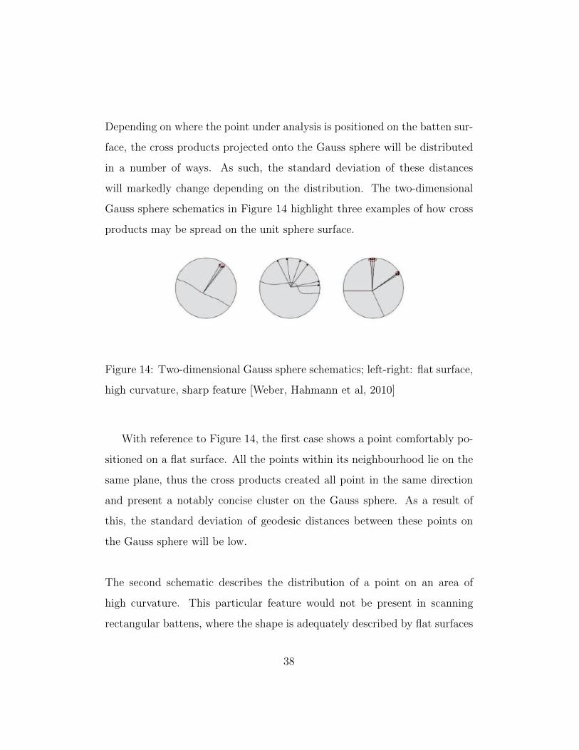
Considerable investigation was carried out to adopt this approach as the
first step in this distortion measurement method. In order to validate the
sharp feature analysis code, point cloud sets of cube surfaces with equally
spaced points were created. The object here, using simplified and somewhat
artificial data, was to confirm that the algorithm worked. Using these test
data sets, good results were achieved, with the code successfully identifying
those points that described the edges of the cube and dismissing those on
the flat surface.
39
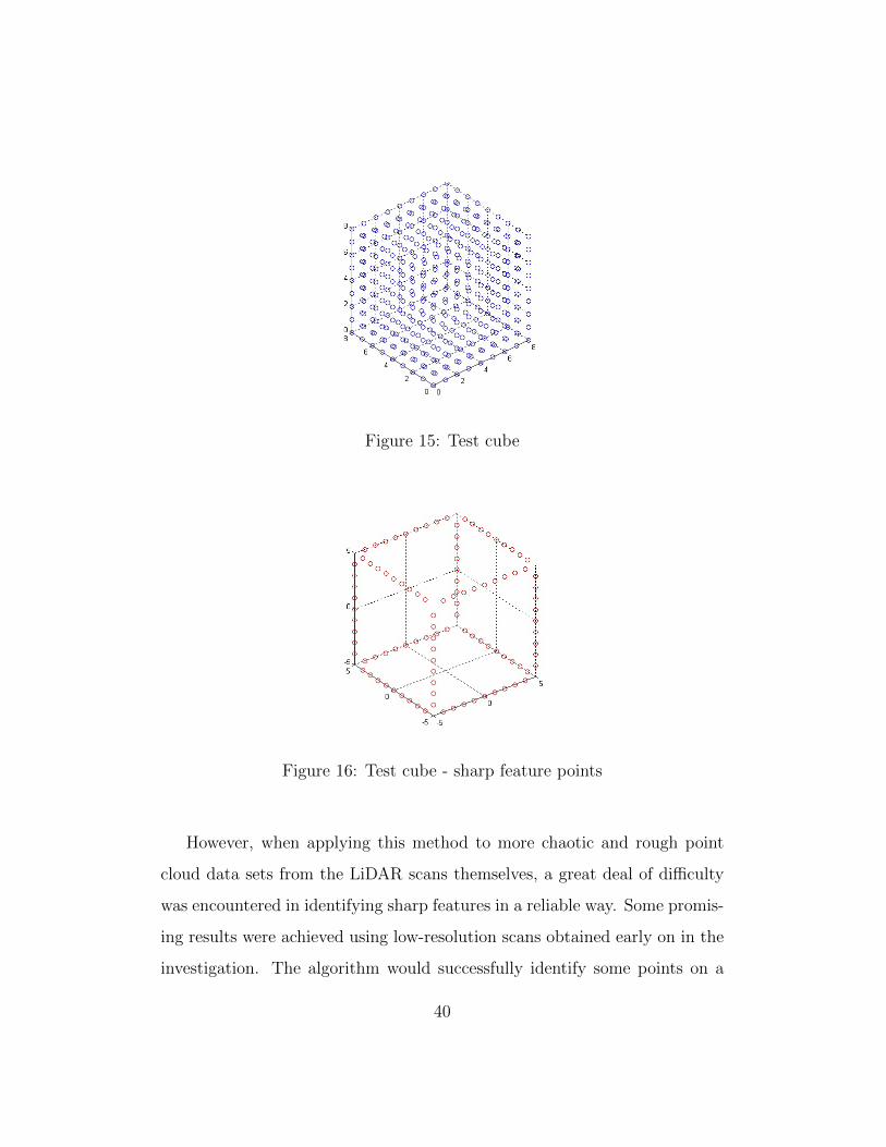
Figure 15: Test cube
Figure 16: Test cube - sharp feature points
However, when applying this method to more chaotic and rough point
cloud data sets from the LiDAR scans themselves, a great deal of difficulty
was encountered in identifying sharp features in a reliable way. Some promis-
ing results were achieved using low-resolution scans obtained early on in the
investigation. The algorithm would successfully identify some points on a
40

sharp feature, and three-dimensional plots of these points would show per-
haps the suggestion of a an edge or a corner. Figure 17 shows the output
from the sharp feature algorithm carried out on a corner section of a batten.
In this instance, the edges of the top and sides surfaces (shown in red and
blue, respectively) were reasonably well identified by the algorithm.
Figure 17: LiDAR data - sharp feature test with batten corner
Nevertheless despite this initially encouraging output, overall the results
from the sharp feature algorithm were unclear and unreliable. There ap-
peared to be too much variability between scans and within individual scans
themselves to create a reliable, ‘universal’ method. Assessing the output
from these sharp feature analyses, it was found that while some sharp feature
41
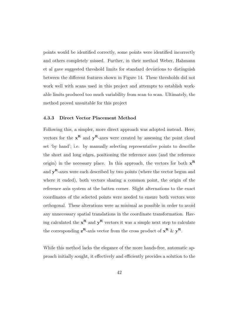
points would be identified correctly, some points were identified incorrectly
and others completely missed. Further, in their method Weber, Hahmann
et al gave suggested threshold limits for standard deviations to distinguish
between the different features shown in Figure 14. These thresholds did not
work well with scans used in this project and attempts to establish work-
able limits produced too much variability from scan to scan. Ultimately, the
method proved unsuitable for this project
4.3.3 Direct Vector Placement Method
Following this, a simpler, more direct approach was adopted instead. Here,
vectors for the xR and yR-axes were created by assessing the point cloud
set ‘by hand’; i.e. by manually selecting representative points to describe
the short and long edges, positioning the reference axes (and the reference
origin) in the necessary place. In this approach, the vectors for both xR
and yR-axes were each described by two points (where the vector begun and
where it ended), both vectors sharing a common point, the origin of the
reference axis system at the batten corner. Slight alternations to the exact
coordinates of the selected points were needed to ensure both vectors were
orthogonal. These alterations were as minimal as possible in order to avoid
any unnecessary spatial translations in the coordinate transformation. Hav-
ing calculated the xR and yR vectors it was a simple next step to calculate
the corresponding zR-axis vector from the cross product of xR & yR.
While this method lacks the elegance of the more hands-free, automatic ap-
proach initially sought, it effectively and efficiently provides a solution to the
42
initial step in the distortion measurement code, creating a ‘best fit’ descrip-
tion of the batten edge as required.
Having established the reference axes in order to carry out a coordinate
transformation from the global system to the reference system, the origins
of both the global LiDAR coordinate system and the reference coordinate
system must be aligned. This is achieved simply by translating the reference
origin from its position in space to a value of (0, 0, 0), and translating the
xR, yR & zR-axes accordingly. These translated vectors are then used to
calculate direction cosines.
4.3.4 Direction Cosine Angles & Transformation Matrix
The reference axis is defined by the following notation:
xR = [Xx, Yx, Zx] (8)
yR = [Xy, Yy, Zy] (9)
zR = [Xz, Yz, Zz] (10)
For each of these vectors, the three direction cosine angles, α, β and γ,
can be calculated to construct a transformation matrix.
[T] =
cosαx cosαy cosαz
cosβx cosβy cosβz
cosγx cosγy cosγz
(11)
Where for a generic vector [a, b, c] direction cosine angles are given as:
43
cosα =a√
a2 + b2 + c2(12)
cosβ =b√
a2 + b2 + c2(13)
cosγ =c√
a2 + b2 + c2(14)
These three angles are calculated for each of the three reference axis vec-
tors.
The transformation from global LiDAR coordinates [X, Y, Z] to equivalent
reference coordinates [XR, Y R, ZR], is given as:xR
yR
zR
= [T].
X
Y
Z
−X0
Y0
Z0
(15)
Where vector [X0, Y0, Z0] represents the spatial translation required to match
the origins of both coordinate systems.
4.3.5 Point Translation & Reference Surface
The convention adopted here of positioning the xR and yR-axes along the
short and long sides of the batten respectively meant that the flat reference
surface onto which the LiDAR points are projected is naturally described
44

on an x-y plane, with the z-component describing the orthogonal distance
through which that point has been projected. Note too in this convention
that a positive z-component describes a point above the reference x-y sur-
face, while a negative z-component describes a point below the reference x-y
surface. A reference grid is built across these projected x-y reference points.
4.3.6 Reference Grid
The concept of a reference grid across which spatial measurements can be
extracted is a salient part of this approach to distortion measurement. The
method of constructing the reference grid presented here, however, evolved
as the investigations progressed.
Before scans had been carried out, it was assumed that a regular rectan-
gular grid of a comparable size to the batten surface would suffice for this
purpose. However, the somewhat varied nature of the batten shapes meant
that this generic approach was not wholly applicable. Some battens pre-
sented marked lateral distortion, their surfaces curving outwards from the
central axis. As a consequence of the projected surfaces curving in the xR
direction, a regularly spaced rectangular grid would not sufficiently represent
the projected surface. These variations in batten shape necessitated a more
flexible approach to constructing each reference grid.
The solution decided upon ensured that the number of points comprising
the reference grid (the ‘resolution’ of the grid) remained the same for each
scan. Spacing of these points in both the xR and yR directions was also
45
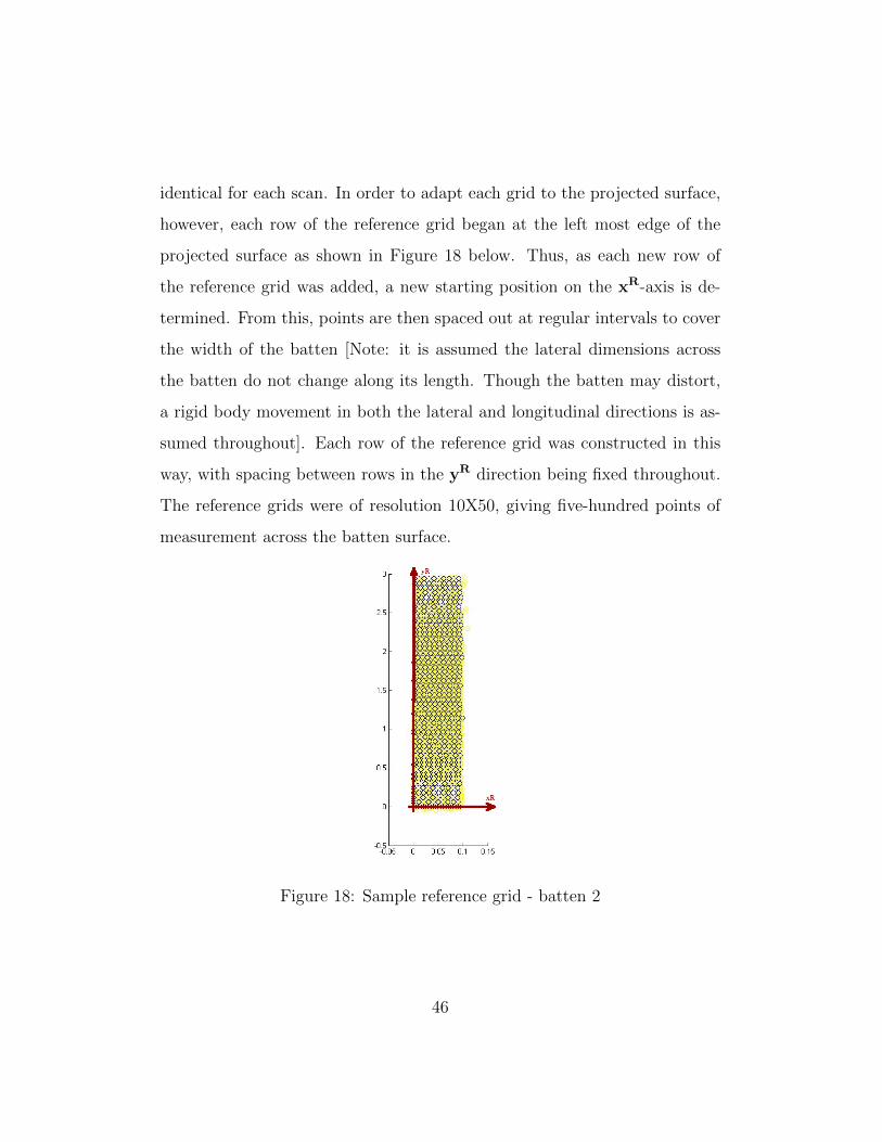
identical for each scan. In order to adapt each grid to the projected surface,
however, each row of the reference grid began at the left most edge of the
projected surface as shown in Figure 18 below. Thus, as each new row of
the reference grid was added, a new starting position on the xR-axis is de-
termined. From this, points are then spaced out at regular intervals to cover
the width of the batten [Note: it is assumed the lateral dimensions across
the batten do not change along its length. Though the batten may distort,
a rigid body movement in both the lateral and longitudinal directions is as-
sumed throughout]. Each row of the reference grid was constructed in this
way, with spacing between rows in the yR direction being fixed throughout.
The reference grids were of resolution 10X50, giving five-hundred points of
measurement across the batten surface.
Figure 18: Sample reference grid - batten 2
46

Batten 2 as shown in Figure 18 provides a typical example of a distorted
surface. The reference grid points (coloured dark blue in the figure) follow the
slight irregularities of the reference surface points (shown in yellow), giving
a closer approximation of the necessary shape.
4.3.7 k-Nearest Neighbour Search & Measurement Extraction
From each point within the reference grid, zR-coordinate values from the sur-
rounding surface points were collated to create a picture of the spatial profile
of the batten. Using open-source neighbourhood search tools developed by
Tagliasacchi, a k-nearest neighbourhood of reference surface points is created
for each point in the reference grid [Tagliasacchi, 2010].
The k-nearest neighbour search algorithm used first organises the data set
(in this instance the LiDAR coordinates) into a k-d tree. The k-d tree is
a data structuring method that employs binary space partitioning to recur-
sively split the feature space into smaller hyper-regions, generating a tree-like
structure in which the original data series is stored [Moore, 1991].
To help ensure a relatively balanced tree structure, the algorithm performs
median splits for each partitioning sequence. The algorithm selects the me-
dian value of all data points within the attribute under consideration. In this
instance, there are three attributes by which each data point is defined: its
x-, y- and z-coordinates. The median-splitting strategy is facilitated by em-
ploying the Heapsort algorithm to sort the data points from least to greatest
value for each of the attributes.
47
In the problem outlined here, dimensionality of the tree is k = 3. As such,
the algorithm cycles through the three attributes of the data series points (x-,
y- and z-coordinates) on each successive partitioning. Moore states that for
uniformly distributed data sets, this median splitting strategy works well.
However, difficulties can arise when the data sets are non-uniformly dis-
tributed [Moore, 1991]. The point cloud data sets used in this thesis were
all of sufficient resolution to ensure they described a uniform distribution
across the batten surfaces.
With the k-d tree structure in place, calculation of the nearest neighbour-
ing points to a query point can be undertaken. This is done by comparing
the attributes of the query point to those values presented at each node
within the tree. The search algorithm follows the path down the appropriate
branches of the tree until those points approximating the query point the
closest are found. The Tagliasacchi algorithm provides flexibility in stipulat-
ing the number and value of query points chosen. In the model given here,
each point in the reference grid represents a query point. In addition, the
number of neighbours (‘k’) is left to the discretion of the user. When the
requisite number of neighbours is found, the search stops accordingly.
From these calculations a two-dimensional array can be built in which the
indexes of the neighbouring points for every reference grid point are stored.
As stated in section 4.3, the orthogonal deviation in the zR direction de-
scribes the position of the batten surface relative to the datum established
48

by the reference surface. Using the zR values for points corresponding to the
neighbourhood indexes, an average orthogonal deviation can be calculated
for each of the reference grid points using the following expression:
zave =
n∑i=1
(zRi∆i
)
n∑i=1
( 1∆i
)(16)
Where:
n = neighbourhood size
zRi = orthogonal deviations of neighbourhood points
∆i = geodesic distance to neighbourhood points
The weighted averaging approach used in Equation 16 whereby distance is
used as the controlling metric was an intuitive choice given that the k-nearest
neighbour search was itself distance-weighted. Each neighbourhood vector
was generated based solely on the spatial proximity of LiDAR scan points to
reference grid points. As such, it was a natural progression when calculating
a weighted average value of orthogonal deviation (zave) that spatial distance
be the controlling variable. However, a number of other distribution func-
tions exist that could be used to carry out a weighted averaging of orthogonal
deviations. In section 7.3, a comparison is carried out showing the impact
of using a generalised Gaussian function as an alternative to the weighted
average in Equation 16.
49
A neighbourhood size of ten was used throughout. This gave good cover-
age around each grid point and did not produce long run times.
Having established an averaged orthogonal deviation for each point on the
reference grid, a profile of how the batten has deformed can be extracted.
By analysing specific groups of deviations and tracking their change along
the batten length (or width), existing feature measurement standards can be
applied to build a description of the batten’s distorted shape. The results of
these calculations are presented in sections 6 where three distortion features
(surface inclination, twist and bow) were calculated using both the FRITS
method and the LiDAR method developed here.
4.4 Alternative Approach To Feature Extraction from
Point Cloud Data Utilising Quadratic Surfaces
Fitting surfaces to describe point cloud data sets has been the focus of many
and diverse areas of research [Levin, 2004]. The preceding section has pre-
sented one approach to achieving this. Naturally, many alternative methods
exist. To provide a wider context to the solution presented in this thesis,
here we highlight an alternative approach to the feature extraction problem.
4.4.1 Quadratic Surfaces
While the distortions that a timber batten can undergo are varied, the final
shape that their surfaces describe can be thought of as an originally rectilin-
ear plane that has been curved and warped within three-dimensional space.
50
As such, the distorted surface to be measured can be approximated by a
quadratic surface. In a general form, quadratic surfaces are defined by the
equation:
Ax2 +By2 + Cz2 +Dxy + Exz + Fyz +Hx+ Iy + Jz +K = 0 (17)
where coefficients A− J are fixed, real constants.
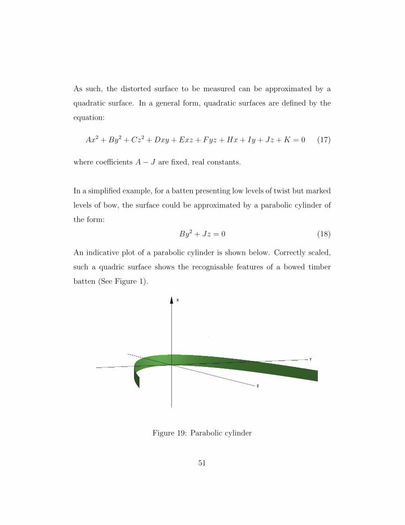
In a simplified example, for a batten presenting low levels of twist but marked
levels of bow, the surface could be approximated by a parabolic cylinder of
the form:
By2 + Jz = 0 (18)
An indicative plot of a parabolic cylinder is shown below. Correctly scaled,
such a quadric surface shows the recognisable features of a bowed timber
batten (See Figure 1).
Figure 19: Parabolic cylinder
51

In order to establish the parameters of Equation (17) and thus define the
batten surface, a least squares approximation method could be employed.
4.4.2 Weighted Least Squares Approximation
A least squares approximation seeks to describe a point-wise data set by an
alternative reference plane such that the sum of squared distances between
the original data set points and the new reference plane is minimised. Min-
imising the distances through which data set points are projected reduces
the error of the final approximated plane. With a localised weighted least
squares approximation, the error is typically weighted by a function of the
Euclidean distances between the data set points and projected points.
Briefly, let the the point data set be defined by N number of points po-
sitioned at xi, in three-dimensional real space where i ∈ [1...N ]. Each point
at fxi is defined by fi. Function f(x) is defined such that the sum of the
squared distances between xi and f(x). However, with a weighted least
squares approach, these distances are weighted by function θ(di), where di is
the Euclidean distance between x and projected point xi. The minimisation
is given as:N∑i=1
θ(d)||fxi − fi||2 (19)
Weighting function θ can be defined in a number of ways; for example, as a
Gaussian: θ = e−d2
h2 (see section 7.3).
52
Function f(x) can be written as:
f(x) = b(x)T .c = b(x).c (20)
where the basis vector b(x) describes the polynomial of the quadratic surface
describing the batten shape, and c is a vector containing the unknown coef-
ficients to be minimised. Taking the partial derivatives of ||fxi−fi||2 results
in a linear system of equations describing the quadratic surface. In order
to evaluate curvatures of the surface, the linear system of equations can be
standardised in its canonical form.
4.4.3 Canonical Form
Describing the polynomial of the quadratic surface in its canonical form helps
to translate the coordinates of the surface points from a global coordinate
system to a local, canonical coordinate system - equivalent to the reference
coordinate system described in this section - independently of the user, re-
moving the need for subjective selection of data points in determining the
reference coordinate system. From here, specific curvatures of the surface
can be calculated, allowing for assessment of the batten surface in accor-
dance with feature measurement standards.
53
5 Experiment Method Description
5.1 Introduction
The scanning experiments focused on comparing distortion measurement
using two different techniques. Seven Sitka spruce battens of dimensions
48.5x102x3000mm were used in total. These were sourced from the BSW
Timber Group’s Carlisle mill. All of the battens had undergone extensive kiln
drying at the Forestry Commission’s Northern Research Station in Roslyn.
Drying was carried out under restrained conditions where each batten had
been secured within a bracket and dried progressively over a number of weeks
to a moisture content of around 12%. Dried in this way, as part of a separate
experiment carried out by colleagues from the University of Glasgow, many
of the battens presented with a variety of marked distortion. Selecting bat-
tens with clear signs of macroscopic distortion provided a more rigorous test
of the new method. All of the test samples were relatively free from knots
and indentations.
5.2 FRITS Experiments
A surface scan of each batten was first carried out using the FRITS frame.
Each batten was scanned lengthwise four times, each scan comprising fifteen
measurements at lengthwise intervals of approximately 0.2m, describing the
surface with sixty data points. This interval length matches that which was
used by Seeling and Merforth [2000] in their initial experiments with their
FRITS frame apparatus.
54
A minimum of two runs is needed to acquire any meaningful results from
the FRITS frame as tracing a single line along the batten provides no oppor-
tunity to interpolate between results to explain the surface shape. Taking
four scans along the batten surface created a measurement area comparable
to the overall width of the surface itself. Dividing this area into four mea-
surements of vertical displacement allowed for a comprehensive averaging
of the overall batten slope. A higher number of measurements would have
provided more input data over which to average. However, given the cum-
bersome nature of the FRITS frame equipment, this would have proved very
time consuming. As such, four lengthwise scans were deemed an appropriate
number to work with.
The lengthwise measurement intervals of 0.2m were approximate to around
1/1000m. These discrepancies were largely due to vibrations and jolting
produced by the scanner as the vertical laser rig moved along its rail. The
stopping mechanism for the vertical laser can be altered manually to cre-
ate shorter or longer distances between measurements, however, as stated
previously, early experiments in establishing the FRITS frame’s competence
worked with this standard of 0.2m producing reliable, reproducible results
[Seeling and Merforth, 2000].
For ease of comparison between FRITS frame and LiDAR scans, it was use-
ful to denote one end of the batten as the ‘top’ (the end at which FRITS
measurement were begun) and the other end as ‘bottom’ (the end at which
FRITS measurements finished). This was then taken into consideration when
55
carrying out LiDAR scans, as described below.
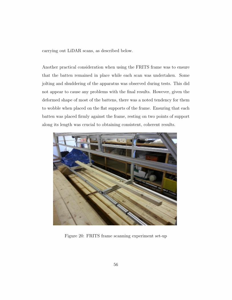
Another practical consideration when using the FRITS frame was to ensure
that the batten remained in place while each scan was undertaken. Some
jolting and shuddering of the apparatus was observed during tests. This did
not appear to cause any problems with the final results. However, given the
deformed shape of most of the battens, there was a noted tendency for them
to wobble when placed on the flat supports of the frame. Ensuring that each
batten was placed firmly against the frame, resting on two points of support
along its length was crucial to obtaining consistent, coherent results.
Figure 20: FRITS frame scanning experiment set-up
56
5.3 LiDAR Experiments
The LiDAR experiments covered in this thesis were carried out using a FARO
Photon 20/120 Laser Scanner. Commercial laser scanners allow for scans to
be made over a range of resolutions, with higher resolutions creating larger
point cloud data samples, thus yielding more detailed depictions of the scan-
ning environment. Increasing the sample size naturally lengthens the scan
time.
In addition to the resolution setting, the spatial limits, both horizontal and
vertical, within which a scan is carried out, must be specified prior to scan-
ning. These limits, or angular area of the scan, again are at the discretion
of the user, depending on the environment being scanned and the nature of
the investigation. An almost complete 360◦ scan is possible (‘Almost’ due to
the inability of the scanner to point completely 180◦ downwards towards the
ground).
Although requiring a somewhat longer set-up than the FRITS frame, scan-
ning each of the battens with the LiDAR scanner was a comparatively quicker
process. While a full FRITS frame would take six to eight minutes, typically
a single LiDAR scan was completed within two minutes.
Selecting a suitable scan resolution was a necessary first step that required
balancing the need for an accurate, detailed description of the battens while
ensuring practical scan times and workable data sets. An extremely high
resolution scan may yield a very accurate point cloud reconstruction of the
57
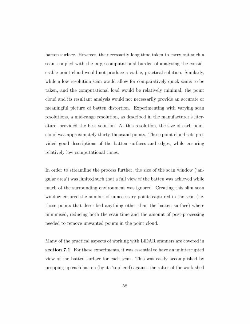
batten surface. However, the necessarily long time taken to carry out such a
scan, coupled with the large computational burden of analysing the consid-
erable point cloud would not produce a viable, practical solution. Similarly,
while a low resolution scan would allow for comparatively quick scans to be
taken, and the computational load would be relatively minimal, the point
cloud and its resultant analysis would not necessarily provide an accurate or
meaningful picture of batten distortion. Experimenting with varying scan
resolutions, a mid-range resolution, as described in the manufacturer’s liter-
ature, provided the best solution. At this resolution, the size of each point
cloud was approximately thirty-thousand points. These point cloud sets pro-
vided good descriptions of the batten surfaces and edges, while ensuring
relatively low computational times.
In order to streamline the process further, the size of the scan window (‘an-
gular area’) was limited such that a full view of the batten was achieved while
much of the surrounding environment was ignored. Creating this slim scan
window ensured the number of unnecessary points captured in the scan (i.e.
those points that described anything other than the batten surface) where
minimised, reducing both the scan time and the amount of post-processing
needed to remove unwanted points in the point cloud.
Many of the practical aspects of working with LiDAR scanners are covered in
section 7.1. For these experiments, it was essential to have an uninterrupted
view of the batten surface for each scan. This was easily accomplished by
propping up each batten (by its ‘top’ end) against the rafter of the work shed
58
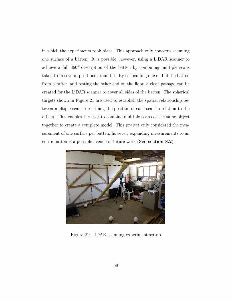
in which the experiments took place. This approach only concerns scanning
one surface of a batten. It is possible, however, using a LiDAR scanner to
achieve a full 360◦ description of the batten by combining multiple scans
taken from several positions around it. By suspending one end of the batten
from a rafter, and resting the other end on the floor, a clear passage can be
created for the LiDAR scanner to cover all sides of the batten. The spherical
targets shown in Figure 21 are used to establish the spatial relationship be-
tween multiple scans, describing the position of each scan in relation to the
others. This enables the user to combine multiple scans of the same object
together to create a complete model. This project only considered the mea-
surement of one surface per batten, however, expanding measurements to an
entire batten is a possible avenue of future work (See section 8.2).
Figure 21: LiDAR scanning experiment set-up
59
5.3.1 Comparison to FRITS Frame
Similar to the FRITS frame, spatial deviations measured by the LiDAR scan-
ner in this method can be assessed in a variety of ways to describe the batten
shape, in accordance with the standards set out in BS EN1310:1997.
As an example, analysing each row of the reference grid provides horizontal
‘slices’ across the batten, describing the overall inclination of the batten sur-
face by which an average angle (θave) can be calculated. This value can be
plotted along the length of the batten, providing a highly detailed description
of batten surface deviation along its entire length. This result can then be
compared to the traditional FRITS frame approach to assess the suitability
of the LiDAR method.
60

6 Results
6.1 Introduction
Section 1.3 introduced standards BS EN 1310:1997 by which distortion fea-
tures can be measured in timber battens. For this project parts of the spatial
data obtained from both measurement techniques (FRITS and LiDAR) were
extracted to allow for comparisons between three measurements of distortion
for each batten.
The first of these measurements, not given in the European Standards, is
a measure of surface inclination along the length of the batten. This is a
standard measurement taken by the FRITS frame and was covered in sec-
tion 3.2. The methodology of FRITS frame measurement, whereby lateral
‘slices’ are taken at regular intervals along a batten length, leads quite nat-
urally to the measurement of surface inclination (θave). With the LiDAR
approach presented here, measuring lateral ‘slices’ along the batten from
each row of the reference grid allows for a straightforward comparison with
the FRITS method.
Measuring how the angle of the batten surface changes along its length in this
way provides an immediate indication of how the surface alters as a whole.
The angle measurements here can dovetail into more specific measurements
of twist as given in the standards. For example, the instance where θave
shows little or no change over a considerable length, i.e. the slope of the
surface remains on a level plane, would indicate a relatively low or negligible
61
degree of twist in the batten.
It should also be noted that for the comparison of FRITS and LiDAR mea-
surements, the focus is on the change in θave along the length of the bat-
ten. Both methods describe distortion by measuring orthogonal deviation
from points on the batten surface to a prescribed datum. With the LiDAR
method presented in this thesis, the datum is set by the placement of the
reference axis, which in itself is unique to each scan. This stands in contrast
to the fixed datum of the FRITS frame approach and would naturally create
orthogonal measurements of different magnitudes. As such, values of θave
for each ‘slice’ would differ between both methods. Nevertheless, with both
approaches, one would expect the overall trend in θave to be the same or
similar, providing both methods are consistent within themselves.
The second measurement is that of twist as described in BS EN 1310:1997
over a length of approximately two metres. The European standards for
timber feature measurement currently lack clarity and are open to various
interpretations of how measurements from a batten should be taken. With
specific reference to twist, the standards only advise measuring orthogonal
deviation over a ‘representative’ two metre length (or the length of the piece).
By the FRITS frame scanning convention shown in Figure 22 the vertical
measurements along lengthwise scans ‘Right’ and ‘Left’ were used to cal-
culate twist in accordance with standards. Each batten was rested on the
FRITS frame supports along its ‘Right’ side as level and as securely as possi-
62
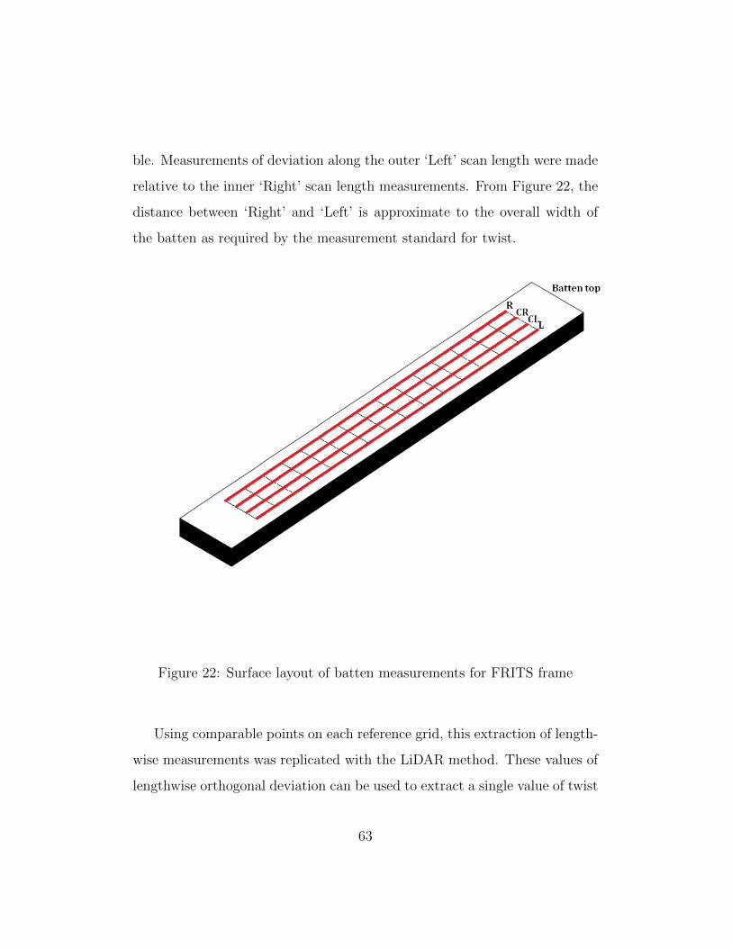
ble. Measurements of deviation along the outer ‘Left’ scan length were made
relative to the inner ‘Right’ scan length measurements. From Figure 22, the
distance between ‘Right’ and ‘Left’ is approximate to the overall width of
the batten as required by the measurement standard for twist.
Figure 22: Surface layout of batten measurements for FRITS frame
Using comparable points on each reference grid, this extraction of length-
wise measurements was replicated with the LiDAR method. These values of
lengthwise orthogonal deviation can be used to extract a single value of twist
63
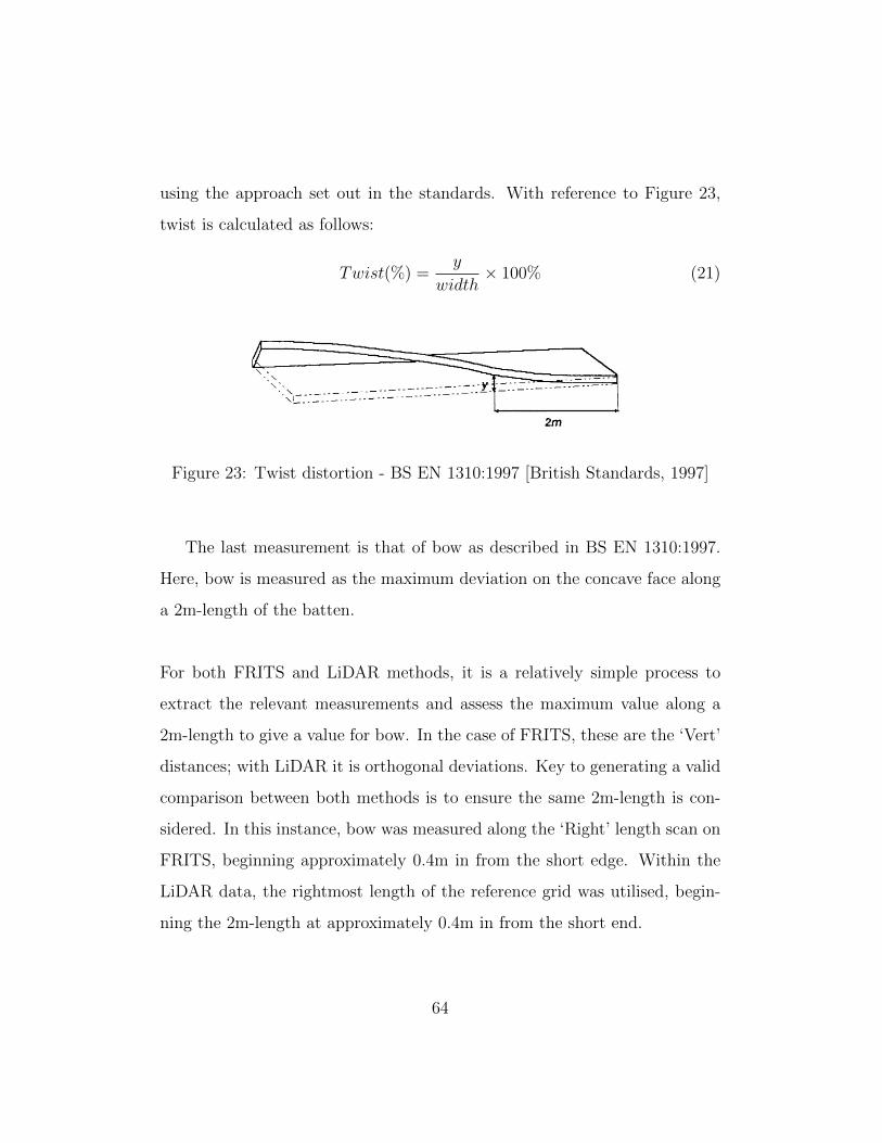
using the approach set out in the standards. With reference to Figure 23,
twist is calculated as follows:
Twist(%) =y
width× 100% (21)
Figure 23: Twist distortion - BS EN 1310:1997 [British Standards, 1997]
The last measurement is that of bow as described in BS EN 1310:1997.
Here, bow is measured as the maximum deviation on the concave face along
a 2m-length of the batten.
For both FRITS and LiDAR methods, it is a relatively simple process to
extract the relevant measurements and assess the maximum value along a
2m-length to give a value for bow. In the case of FRITS, these are the ‘Vert’
distances; with LiDAR it is orthogonal deviations. Key to generating a valid
comparison between both methods is to ensure the same 2m-length is con-
sidered. In this instance, bow was measured along the ‘Right’ length scan on
FRITS, beginning approximately 0.4m in from the short edge. Within the
LiDAR data, the rightmost length of the reference grid was utilised, begin-
ning the 2m-length at approximately 0.4m in from the short end.
64
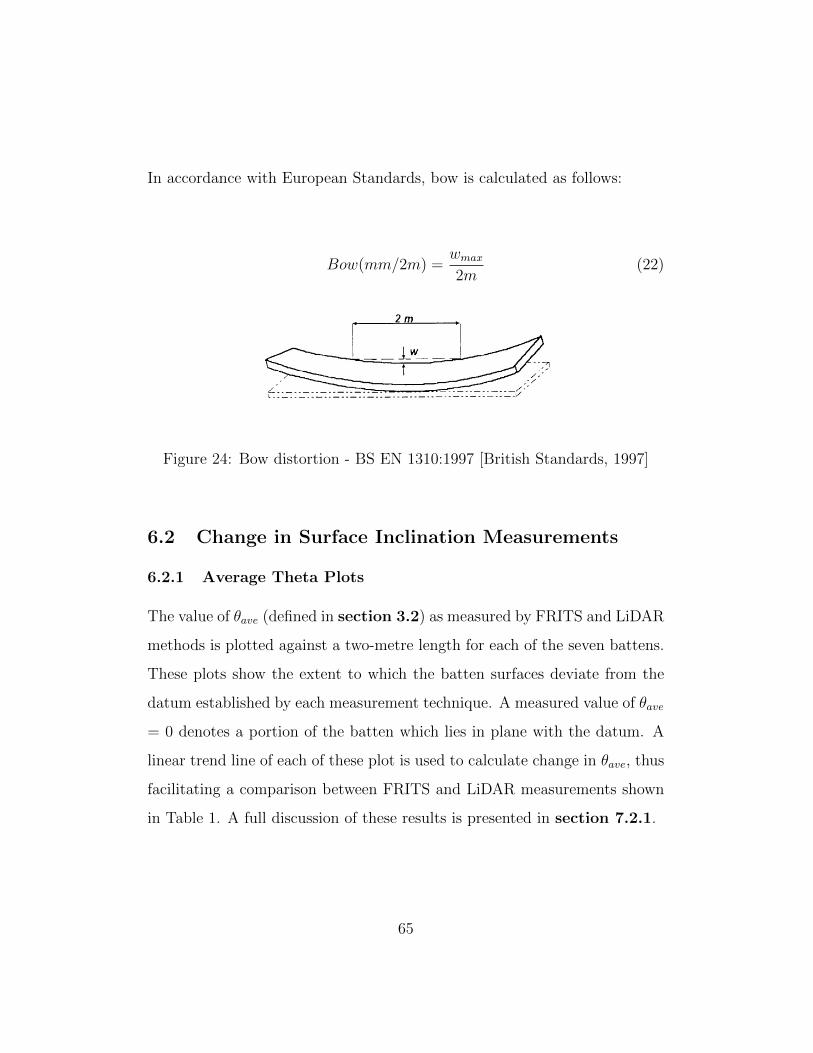
In accordance with European Standards, bow is calculated as follows:
Bow(mm/2m) =wmax
2m(22)
Figure 24: Bow distortion - BS EN 1310:1997 [British Standards, 1997]
6.2 Change in Surface Inclination Measurements
6.2.1 Average Theta Plots
The value of θave (defined in section 3.2) as measured by FRITS and LiDAR
methods is plotted against a two-metre length for each of the seven battens.
These plots show the extent to which the batten surfaces deviate from the
datum established by each measurement technique. A measured value of θave
= 0 denotes a portion of the batten which lies in plane with the datum. A
linear trend line of each of these plot is used to calculate change in θave, thus
facilitating a comparison between FRITS and LiDAR measurements shown
in Table 1. A full discussion of these results is presented in section 7.2.1.
65
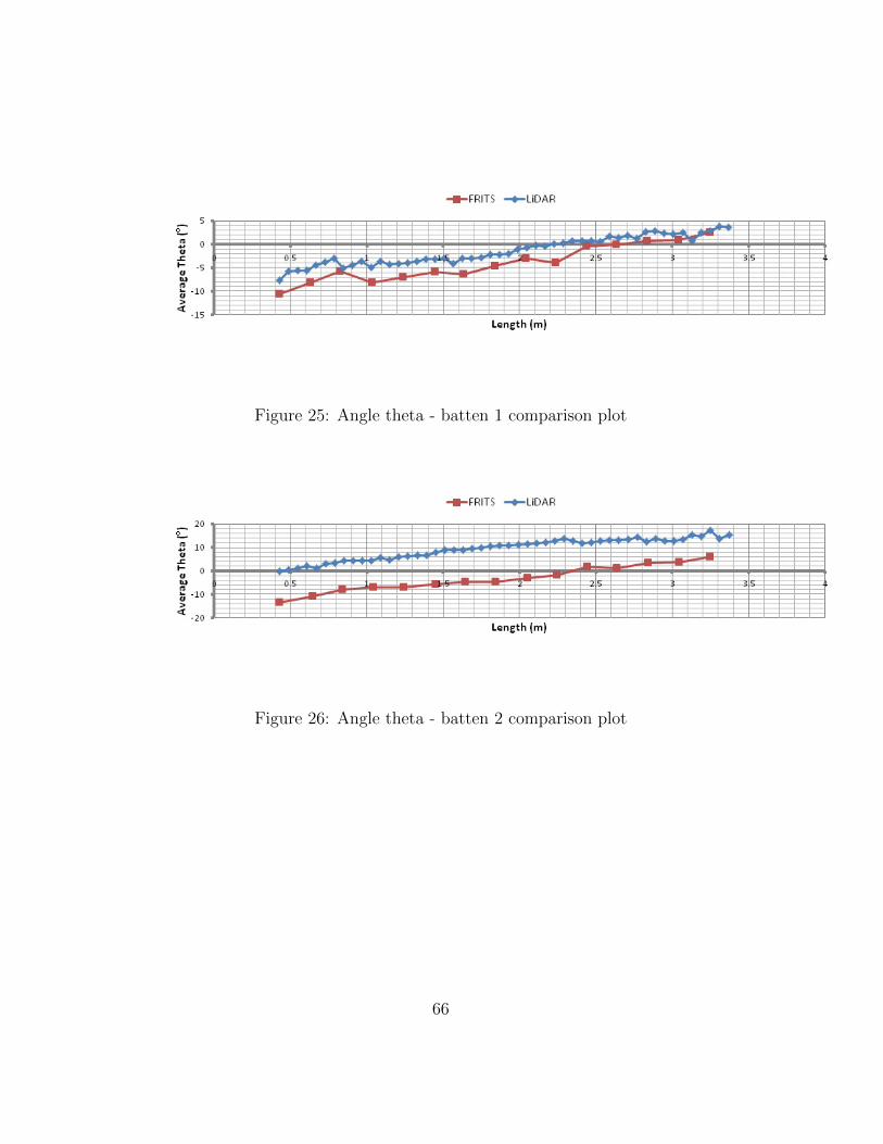
Figure 25: Angle theta - batten 1 comparison plot
Figure 26: Angle theta - batten 2 comparison plot
66
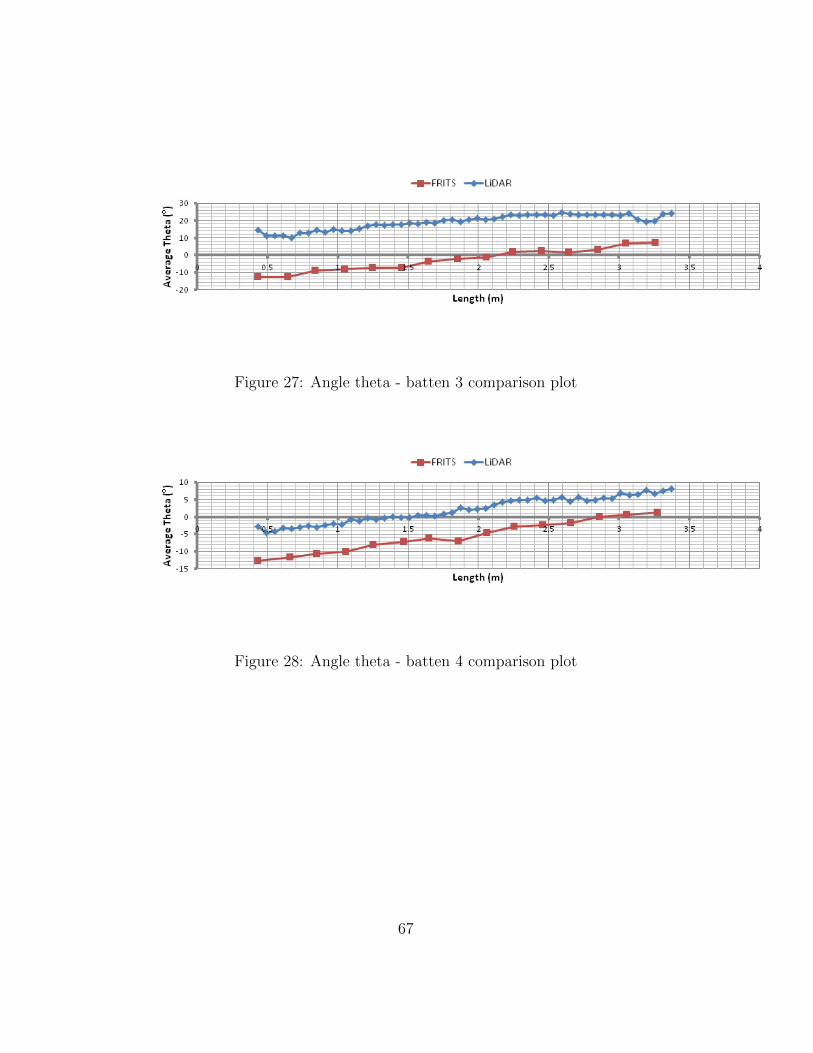
Figure 27: Angle theta - batten 3 comparison plot
Figure 28: Angle theta - batten 4 comparison plot
67
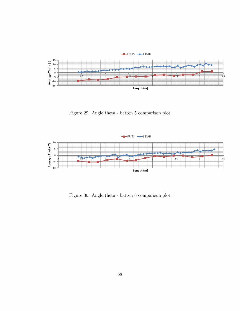
Figure 29: Angle theta - batten 5 comparison plot
Figure 30: Angle theta - batten 6 comparison plot
68
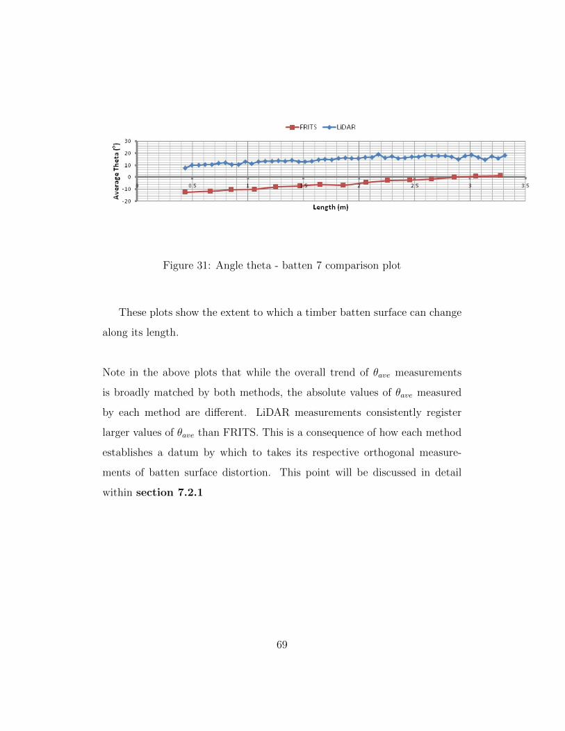
Figure 31: Angle theta - batten 7 comparison plot
These plots show the extent to which a timber batten surface can change
along its length.
Note in the above plots that while the overall trend of θave measurements
is broadly matched by both methods, the absolute values of θave measured
by each method are different. LiDAR measurements consistently register
larger values of θave than FRITS. This is a consequence of how each method
establishes a datum by which to takes its respective orthogonal measure-
ments of batten surface distortion. This point will be discussed in detail
within section 7.2.1
69
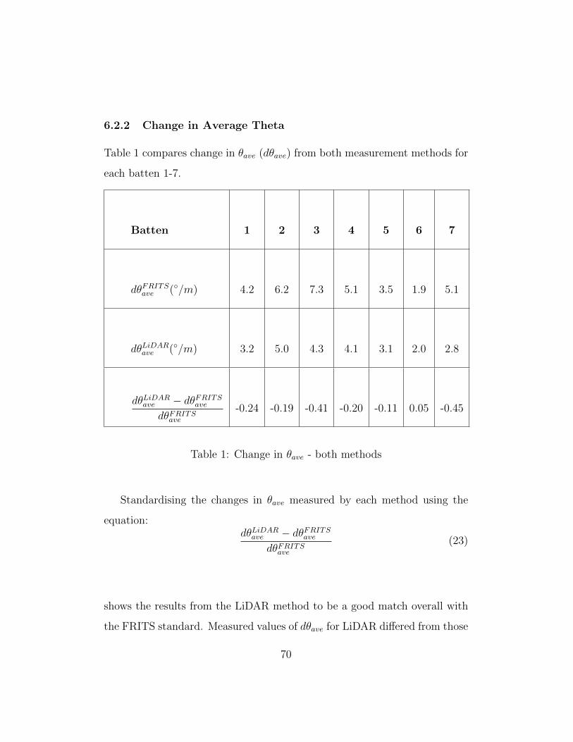
6.2.2 Change in Average Theta
Table 1 compares change in θave (dθave) from both measurement methods for
each batten 1-7.
Batten 1 2 3 4 5 6 7
dθFRITSave (◦/m) 4.2 6.2 7.3 5.1 3.5 1.9 5.1
dθLiDARave (◦/m) 3.2 5.0 4.3 4.1 3.1 2.0 2.8
dθLiDARave − dθFRITS
ave
dθFRITSave
-0.24 -0.19 -0.41 -0.20 -0.11 0.05 -0.45
Table 1: Change in θave - both methods
Standardising the changes in θave measured by each method using the
equation:dθLiDAR
ave − dθFRITSave
dθFRITSave
(23)
shows the results from the LiDAR method to be a good match overall with
the FRITS standard. Measured values of dθave for LiDAR differed from those
70

of the FRITS frame by a mean value of −0.22◦/m with a standard deviation,
σ = 0.17◦/m. A discussion of these results is presented in section 7.2.1.
6.3 Twist Measurements
Using the convention introduced in section 6.1 a single of value of twist was
extracted from each of the seven battens by means of both the FRITS and
LiDAR scanning methods. The results are summarised in Table 2 below.
Batten 1 2 3 4 5 6 7
TwistFRITS(%) 0.0 3.1 2.9 -4.2 -5.0 0.0 -3.0
TwistLiDAR(%) 0.1 2.1 4.5 -1.0 -1.1 0.2 -3.0
TwistLiDAR − TwistFRITS
TwistFRITS/ -0.32 +0.55 -0.76 -0.78 / 0.00
Table 2: Twist - both methods
Measured values of Twist for LiDAR differed from those of the FRITS
frame by a mean value of −0.26% with a standard deviation, σ = 0.56%. A
discussion of these results is given in section 7.2.2.
71
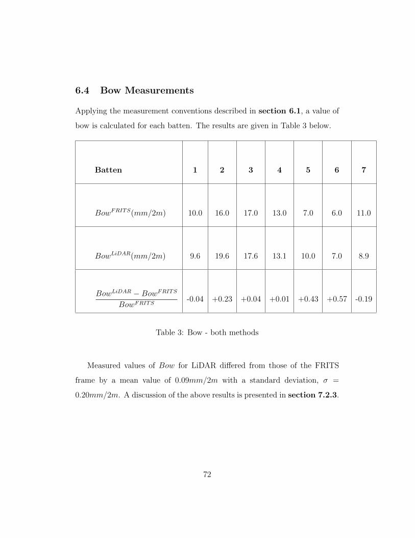
6.4 Bow Measurements
Applying the measurement conventions described in section 6.1, a value of
bow is calculated for each batten. The results are given in Table 3 below.
Batten 1 2 3 4 5 6 7
BowFRITS(mm/2m) 10.0 16.0 17.0 13.0 7.0 6.0 11.0
BowLiDAR(mm/2m) 9.6 19.6 17.6 13.1 10.0 7.0 8.9
BowLiDAR −BowFRITS
BowFRITS-0.04 +0.23 +0.04 +0.01 +0.43 +0.57 -0.19
Table 3: Bow - both methods
Measured values of Bow for LiDAR differed from those of the FRITS
frame by a mean value of 0.09mm/2m with a standard deviation, σ =
0.20mm/2m. A discussion of the above results is presented in section 7.2.3.
72
7 Comparative Analysis
7.1 Practical Aspects of Feature Measurement Exper-
iments
Here, a comparative overview of some of the practical aspects of both mea-
surement techniques is presented.
7.1.1 FRITS Experiments
The FRITS frame has the advantage of being a proven, established measure-
ment technique. Set-up time of the apparatus itself is relatively minimal as
the equipment is a stationary unit; and after a brief introduction, its use is
largely straightforward. Measurements from both lasers can be input into a
spread sheet immediately they have been taken using a Bluetooth connection
between both lasers and a laptop. Given the repetitive and formatted nature
of the scanning procedure it is possible to build up output calculations of
distortion features while the scan is taking place, giving a finalised data set
upon completion of the scan. This requires each batten to be scanned in the
same way.
Scan time for each batten was around six to eight minutes. This included
ensuring each batten was positioned firmly in place within the frame, carry-
ing out test runs to ensure the vertical laser was on target along the length
of the timber, as well as dealing with the inevitable glitches and interrupted
signals incurred while using Bluetooth. This timescale only applies to the
scanning of one surface per batten.
73
The size and bulk of the frame apparatus itself limits where and when the
measurements can be carried out. The frame is a static piece of equipment
and as such must always be worked around. Further, the manual nature of
positioning the FRITS frame lasers incurs inaccuracies in establishing ex-
actly where each laser measurement is positioned on the batten surface. The
method assumes that the edge of the batten runs parallel to the direction
along which the laser travels. This may be a suitable assumption for battens
presenting little deviation from the central axis. However, this can become
less justifiable as batten deformation increases.
7.1.2 LiDAR Experiments
The technical requirements for using a LiDAR scanner are somewhat greater
than those of the FRITS frame. A trained technician is needed for both the
set-up of the apparatus, as well as the post-scan editing required. Once set-
up correctly, scan time for the chosen resolution was less than two minutes.
If multiple scans of a batten are to be taken, the method only requires ac-
cess to all sides of the batten. With this accounted for, resetting for another
scan takes very little time. While markedly quicker to scan than the FRITS
frame, LiDAR scanning does require a certain amount of post-processing of
the point cloud data to eliminate unnecessary points. Additional manipula-
tion is needed if multiple scans are to be combined.
Unlike the FRITS frame, LiDAR scanning can be carried out wherever there
is room to comfortably manoeuvre the batten and the LiDAR unit. Weather
74

permitting, and with adequate power supply, it can also be performed out-
side, freeing it from the static constraints of the Freiburg method. Of par-
ticular note, LiDAR scanning does not require the often cumbersome and
potentially costly transport of timber battens to the scan site. Rather, the
relatively portable scanning equipment and battery supply can be taken to
where they are needed, freeing up the measurement process and allowing a
more flexible, adaptive approach to distortion measurement.
With the LiDAR method, however, measurements of distortion cannot be
extracted directly and automatically from the raw data as in the FRITS
method. Once the point cloud has been finalised, further information must
be extracted from the data before distortion measurements can be taken.
A datum from which distortion can be measured must be established first.
With the FRITS frame scans, this datum is set automatically by the frame
itself and remains constant for each experiment. However, each time a scan is
carried out using LiDAR, the datum changes with the position of the scan-
ner and the batten being measured. Calculating a reference surface from
which deviations can be measured is a necessary first step in the new LiDAR
method, and is unique for each scan (See section 4.3 for a full explanation
of the distortion code).
This additional analysis is a consequence of the substantially greater amount
of input data gained from the LiDAR method as compared to the FRITS
frame. The FRITS frame experiments took sixty measurements of each bat-
ten surface, whereas the point cloud used to describe each batten with the
75

LiDAR scanner consisted of around thirty-thousand points. Managing these
larger figures and extracting meaningful measurements from them will there-
fore undoubtedly be subject to greater computational requirements.
However, the LiDAR scan does provide a much more comprehensive de-
scription of each unique batten surface: in stark contrast to the pointwise,
interpolative measurements of the FRITS frame. Further, set-up and scan
times for the LiDAR are considerably shorter and less tedious than those of
the FRITS. Use of the FRITS frame requires positioning the batten within
the frame such that a suitable number of points can be measured; the start-
ing position for each scan length and the distances between them must be
measured by hand, and a test run for each new scan length must be carried
out to ensure the laser remains comfortably on the batten surface through-
out. All of which generates an unavoidably lengthy scanning procedure.
In contrast, positioning of the batten for LiDAR scanning requires only that
the scanner receives an uninterrupted view of the batten surface and that
the batten remains stationary. No manual measurements need be taken of
the batten during LiDAR scanning as these can be extracted from the point
cloud data as necessary. Combined, these features allow for a greater num-
ber of battens to be scanned in a much shorter period of time compared to
the FRITS frame. From a practical standpoint LiDAR scanning provides a
quicker, more efficient solution to feature measurement.
76
7.1.3 Measurement Errors
The FRITS frame apparatus utilised two Leica DISTO lasers with a certified
accuracy of ±2mm. For the LiDAR experiments a FARO Photon 20/120
Laser Scanner was used, also with a certified accuracy of ±2mm, as per the
manufacturer’s literature. In discussing the accuracy of laser scanning tech-
nologies, the range over which measurements are taken is important. Given
the dimensions of the FRITS frame, vertical measurements of displacement
were taken from around one meter from the surface of the batten. With
the LiDAR set-up used, the scanner was similarly placed around one to two
meters from the batten for each experiment. In this regard, the FRITS
frame apparatus does ensure consistent, standardised measurements, while
the movable nature of LiDAR opens itself up to discrepancies in the range
over which it scans. However, the portable nature of the LiDAR is one of
the things that recommends it over the static FRITS approach.
Further, the FRITS frame is subjected to a noticeable degree of vibration
as the vertical laser moves along its track. Quantifying the impact of this
movement on final accuracy is difficult. However, it is not inconceivable that
a markedly distorted batten - say, for example, a batten presenting a signifi-
cant degree of bow - could be disturbed from its resting position on the frame
as the laser moves down the track. Any accidental movement of the batten
during scanning could understandably produce inaccurate results. The issue
of vibration is not a problem met with by the LiDAR scanner. Provided the
scanner is positioned on a solid, stable footing, the equipment presents no
noticeable degree of vibration.
77
Output from the FRITS frame lasers was given to the nearest 1mm, whereas
LiDAR output was to the nearest one-hundredth of a millimetre. To ease
comparison and to avoid spuriously ‘precise’ results, all final distortion fea-
ture measurements were given to one decimal place for both methods. This
corresponded to batten measurements for bow and twist being taken to the
nearest millimetre. For measurements of angle theta, the relevant batten
measurements used in the calculations were also rounded to the nearest mil-
limetre. Measurements were restricted in this way to allow easy comparison
with the FRITS frame measurements, whose limits of accuracy only extended
to the level of a millimetre. Further, specifications for distortion limits pro-
vided in the standards are only given to the nearest millimetre [BS EN
14081-1, 2005].
While the LiDAR produces measurements to a finer degree of detail than
the FRITS, the lower specification of the FRITS equipment in addition to
the accuracy prescribed in the standards mean that a comparison between
the two methods was restricted to the FRITS frame’s lesser measurement
length scale. This being said, some insight was gained by the finer level de-
tail of the LiDAR. For instance, two battens (battens 1 and 6) in the sample
presented with 0.0% twist when measured by FRITS. Given that the battens
were selected due to their failing of visual inspection, it seems unlikely that
any of the battens did not present with some degree of twist. More likely
rather is that the lower accuracy of the FRITS frame did not register enough
of a discrepancy between vertical measurements at the millimetre scale to
78
generate a value of twist. However, with the LiDAR scanner a small de-
gree of twist was registered in both battens. This potentially suggests that
both its increased point density and measurement accuracy allows the Li-
DAR to recognise subtle features of batten shape not currently afforded by
the FRITS.
7.2 Distortion Measurements
7.2.1 Change in Surface Inclination
Measurements of change in surface inclination as achieved by the LiDAR
method compared well against those measured by the FRITS frame stan-
dard. However, with the exception of a small portion of batten 1, LiDAR
measurements of θave were larger than those of FRITS to a greater or lesser
degree. This difference in magnitude is a result of the nature by which each
method generates its respective datums, relative to the batten surface.
In the case of the FRITS frame the process is consistent and automatic
for each scan. Vertical measurements are taken from the laser affixed to
the upper supports of the frame structure. Each batten is lain on the lower
frame supports, which run parallel to those above, while ensuring that three
points of support are maintained. As such, the surface on which each batten
sits is in plane with that from which measurements are taken. Thus, if a
batten presents with only relatively minor distortion out of plane from the
supports, then relatively smaller values of θave will be recorded. With ref-
erence to the results presented in sections 6.2.1-2, batten 6, for instance,
79

shows a batten largely in plane with the FRITS structure, with a low value
of dθave = 1.9◦/m. It is interesting to note that with this low value of dθave,
batten 6 recorded a twist value of 0%. Conversely, batten 3 recorded a larger
value of dθave = 7.3◦/m, and a subsequently larger value of twist = 2.9%.
With the LiDAR method presented here, however, the position of the datum
is much more arbitrary, tailored each time to the batten under consideration.
The reference surface from which deviations are measured is described by rel-
atively few points along the short and long edges of the batten. Indeed, both
the xR and yR axes were defined by just three points in total: one shared
point at the approximate corner of the ‘top’ end of the batten which served
as the reference origin, and one point along the adjacent short and long edges
to define the xR and yR axes respectively.
This point-wise approach stands in contrast to the FRITS method. In this
instance, the extent to which the batten has distorted will determine how
it rests on the support surface; however, that surface will always remain in
plane with the surface from which measurements are taken. On the other
hand, the LiDAR is much more susceptible to generating a reference sur-
face that is markedly more out of plane with the batten surface itself. This
seems to be the case in the measurements of θave, where the magnitudes of
angle θave were consistently larger for LiDAR than with FRITS. Figure 32
below compares how a difference in orientation between FRITS and LiDAR
measurements can lead to a difference in magnitude for avalue of θave at an
arbitrary point along the batten length.
80
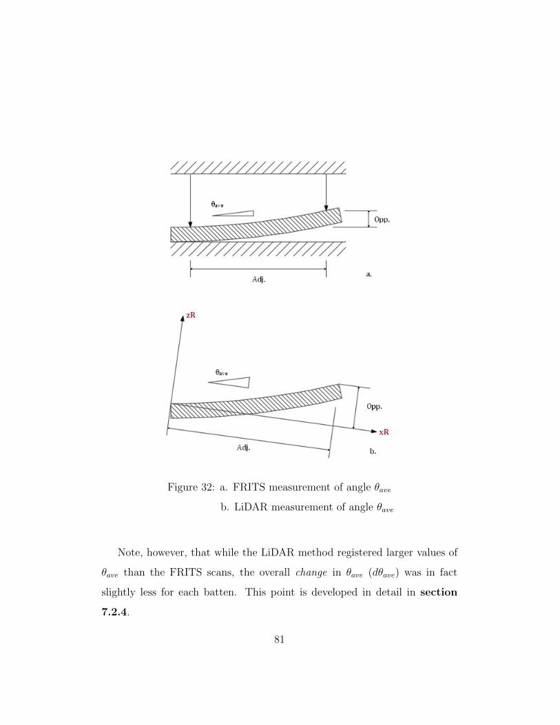
Figure 32: a. FRITS measurement of angle θave
b. LiDAR measurement of angle θave
Note, however, that while the LiDAR method registered larger values of
θave than the FRITS scans, the overall change in θave (dθave) was in fact
slightly less for each batten. This point is developed in detail in section
7.2.4.
81

As was to be expected with using such a large data set, the LiDAR scans
generated much more variable measurements of surface inclination, as the
plots of average theta in Figures 25-31 attest. Still, even with the far larger
amount of measurement, a linear trend line applied to the measurements of
angle θave show relatively smooth curves, comparing well with the much more
limited measurements produced by the FRITS scans. This smoothness could
be improved further by increasing the resolution of the reference grid to gen-
erate an even greater number of measurements. It must be noted, however,
that this increase would naturally entail a greater computational burden.
This point of reference grid resolution is developed further in section 8.2.
Across all seven battens, the LiDAR method was able to accurately and
reliably reproduce dθave results gained from the FRITS standard.
7.2.2 Twist
Overall, measurements of twist gained from the new LiDAR approach com-
pared well with those achieved by FRITS. Unlike measurements of dθave,
where trends over the length of the batten were considered, single values
of twist were extracted at a specific length from each batten end. In this
way, discrepancies between measurement datums of both methods discussed
above were somewhat more influential in determining degrees of twist than
was apparent in measurements of surface inclination.
Prescriptions for measuring twist in accordance with European Standards
82

require one long side of the batten to be laid on a flat surface while the
height of the opposite long side is recorded at a length of two metres from
the batten end. This height (y) is divided by the batten width to give a
measure of twist, with the final value being expressed as a percentage.
In the FRITS frame experiments, each batten was rested on the frame sup-
ports along its ‘Right’ side, as per the convention described in section 6.1.
Measurements of height were then taken from the opposing ‘Left’ edge. In
this way, the ‘Right’ side of each batten was prescribed as being the lower
side, with height measurements (y) recorded relative to it. With the LiDAR
method, however, the reference axes were positioned such that yR axis was
aligned along the ‘Left’ long side of the batten. By this convention, the ’Left’
long side of each was prescribed as the lower side. This difference in orienta-
tion had to be considered when extracting values of ‘y’ from point cloud data
in order to match the convention established by FRITS. This ensured that
the LiDAR data matched the FRITS data in terms of its sign convention.
However, the magnitude of twist measurements differed to varying degrees
across the sample battens.
These differences in magnitude of twist as measured by LiDAR in comparison
to FRITS were largely a result of the arbitrary placement of the reference
surface discussed above. Three out of the seven battens scanned measured
a value of twist less that measured by FRITS, with a fourth giving batten
matching the value of twist (rounded to one decimal place). This corresponds
strongly with the trend observed with measurements of change in surface in-
83
clination whereby the LiDAR consistently recorded lower values than the
FRITS frame.
In a similar way to measurements of the change in surface inclination, mea-
surements of twist essentially record a change in height across the batten
surface- not lengthwise, as with surface inclination, but rather laterally across
the batten width. In this way, the height of one side of the batten (y) is mea-
sured by it’s relative position to the height of the other side which is assumed
to be on a flat, level surface. Where the reference axes are not fully aligned
with the plane of the batten surface, values of orthogonal deviation used to
calculate height ‘y’ may incur additional offsets making a faithful comparison
with the more standardised FRITS method more challenging.
7.2.3 Bow
Many of the issues raised in the comparisons between measurements of both
surface inclination and twist obtain for bow. Overall, measurements of bow
using LiDAR matched strongly with those gained from FRITS. As discussed
above, the LiDAR measurements presented differing magnitudes of bow com-
pared to those measured by FRITS; however, with bow measurements, these
differences were relatively small across the sample set.
7.2.4 Distortion Measurements Summary
Concerning the magnitudes of distortion values, in five of the seven battens
scanned, the LiDAR method recorded a larger value of bow than FRITS. It
is interesting to note that of the four feature measurement types considered
84
here, surface inclination (θave) and bow generally recorded larger values with
the LiDAR method than the FRITS; while both change in surface inclination
(dθave) and twist tended to record lower values for the LiDAR method. These
trends may provide insight into how the reference axis placement performs
and help guide efforts to more a standardised, reliable approach in the future.
For now, these discussions will help inform any comparisons between FRITS
and LiDAR
Those feature measurements that recorded larger values with the LiDAR
model (θave and bow) considered only single measurements at a specific point
on the batten surface. In the case of θave this was the angle of the surface
at prescribed intervals. With bow it was the maximum deviation from the
longitudinal axis along a two metre length of one edge of the batten. These
measurements did not consider any relative change in the batten surface,
nor the relationship of one portion of the batten with another. Rather, they
concerned only direct measurements of the batten relative to the reference
surface. Surface inclination with the LiDAR method was a measure of the
slope of the batten surface relative to the reference surface. Similarly, in mea-
suring deviations along a two meter-length of one long edge and selecting the
maximum value to calculate bow, the final result recorded was directly de-
pendent on the spatial relationship of the batten and reference surface.
Conversely, measurements of dθave and twist recorded relationships of the
batten relative to itself. Change in surface inclination considered how the
slope of the batten altered from one end to the other along the longitudinal
85
axis. Twist considered the projecting height of one side of the batten rela-
tive to the other side. In this way, the relationship between the batten and
it’s measurement datum was of little consequence. Only changes across the
batten were measured.
As such, in assessing the discrepancies brought about by the arbitrary place-
ment of the reference axes, the issue of axis positioning is more pertinent to
measures of θave and bow. Additionally, from the definitions established in
the European standards, measurement of spring would also be dependent on
the placement of the reference axis. In these instances, a formalised, univer-
sal placement system would be required to provide more reliable comparisons
between LiDAR and FRITS. With measurements of change in surface inclina-
tion and twist (and cup as per European standards), however, reference axis
placement and orientation becomes less important. In this way, a stronger
comparison can be made between results from the new LiDAR method and
the FRITS frame.
Notwithstanding some of the issues raised regarding the comparison between
FRITS and LiDAR, it is interesting to note that both methods recorded an
apparent correlation between measured values of change in surface inclina-
tion, twist and bow. From the relatively small selection of batten samples
used in this thesis, a higher measurement of change in surface inclination
tended to correspond to greater values of both twist and bow. Both FRITS
and LiDAR recorded the highest values of each of these measurements in
battens two and three. For lower values of dθave, the comparison breaks
86
down somewhat with LiDAR measurements of twist. Among the batten
samples, FRITS recorded a lowest value of dθave in batten 6 (1.9◦/m). Cor-
respondingly, FRITS measured the lowest values of twist and bow in batten
6 (0% and 6mm/2m, respectively). For twist measurements, this was not
fully captured with the LiDAR method. However, the trend was replicated
much more reliably with measurements of bow, where again one of the lowest
measurements were recorded in batten 6 (9.4mm/2m).
7.3 Weighted Averaging Method - Comparison with
Gaussian Weighting Function
In Section 4.3.7 a method was introduced by which a measure of orthogonal
deviation could be estimated for each point on the reference grid by averaging
the orthogonal deviations of the surrounding LiDAR points. However, the
weighted averaging method used, shown in Equation 16, is only one possible
method and others exist. Given that the weighting method is used to estab-
lish final orthogonal deviations across the reference grid points, it’s influence
on the measurements extracted from the LiDAR model is clear. For this rea-
son, an investigation was carried out to assess what impact was made on final
distortion measurements by using an alternative weighted averaging fucntion.
Alexa et al. [2003] describe a typical Gaussian weight function that can
be applied to averaging procedures with point data sets. The weight func-
tion is as follows:
87
Wi = e∆2i
H2 (24)
Where:
∆i = geodesic distance of neighbourhood point to reference grid point
H = parameter representing the geodesic distances between points within
the neighbourhood
Levin [2004] specifies the ‘H’ parameter as the average distance between
data points. Accordingly, the mean spacing between points within each Li-
DAR scan was used for the value of ‘H‘.
As can be seen, the influence a point has in determining the final orthogonal
deviation falls off exponentially the further the point is from the reference
grid point. Thus, the averaged measurement tends to greatly favour those
points closer to the measurement point.
The average orthogonal deviation of each reference grid point is calculated
by multiplying the orthogonal deviation of each neighbourhood point by the
above weighting function and summing. This is shown in Equation 25.
zave =n∑
i=1
WizRi (25)
88
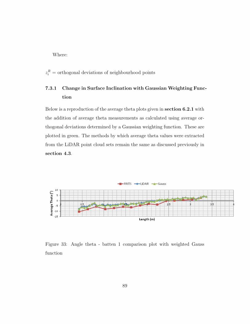
Where:
zRi = orthogonal deviations of neighbourhood points
7.3.1 Change in Surface Inclination with Gaussian Weighting Func-
tion
Below is a reproduction of the average theta plots given in section 6.2.1 with
the addition of average theta measurements as calculated using average or-
thogonal deviations determined by a Gaussian weighting function. These are
plotted in green. The methods by which average theta values were extracted
from the LiDAR point cloud sets remain the same as discussed previously in
section 4.3.
Figure 33: Angle theta - batten 1 comparison plot with weighted Gauss
function
89
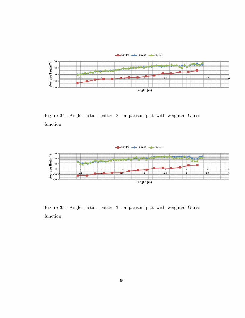
Figure 34: Angle theta - batten 2 comparison plot with weighted Gauss
function
Figure 35: Angle theta - batten 3 comparison plot with weighted Gauss
function
90

Figure 36: Angle theta - batten 4 comparison plot with weighted Gauss
function
Figure 37: Angle theta - batten 5 comparison plot with weighted Gauss
function
91
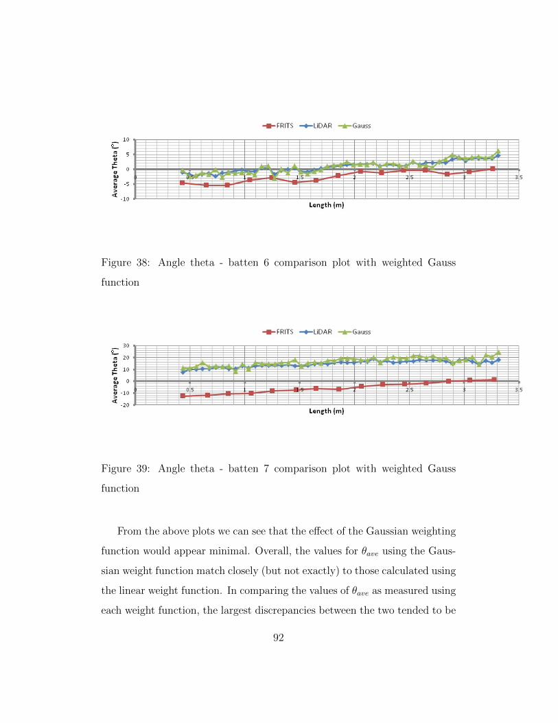
Figure 38: Angle theta - batten 6 comparison plot with weighted Gauss
function
Figure 39: Angle theta - batten 7 comparison plot with weighted Gauss
function
From the above plots we can see that the effect of the Gaussian weighting
function would appear minimal. Overall, the values for θave using the Gaus-
sian weight function match closely (but not exactly) to those calculated using
the linear weight function. In comparing the values of θave as measured using
each weight function, the largest discrepancies between the two tended to be
92
within those measurements taken at the ends of the battens. These areas at
the ends of each batten tended to be where the fit of the reference grid to
the projected reference surface was somewhat less precise and the reference
grid rows did not align exactly with the often rather scattered arrangement
of the reference surface points. As such, the neighbourhood searches along
these rows struggled to produce a cogent measurement of orthogonal devia-
tion. These discrepancies seem to have been further affected by the change
of weight function.
As before, a measure of the change in surface inclination was calculated
with the Gaussian weight function. These results are summarised in Table 4
below, along with the original values obtained from the FRITS and LiDAR
methods.
93
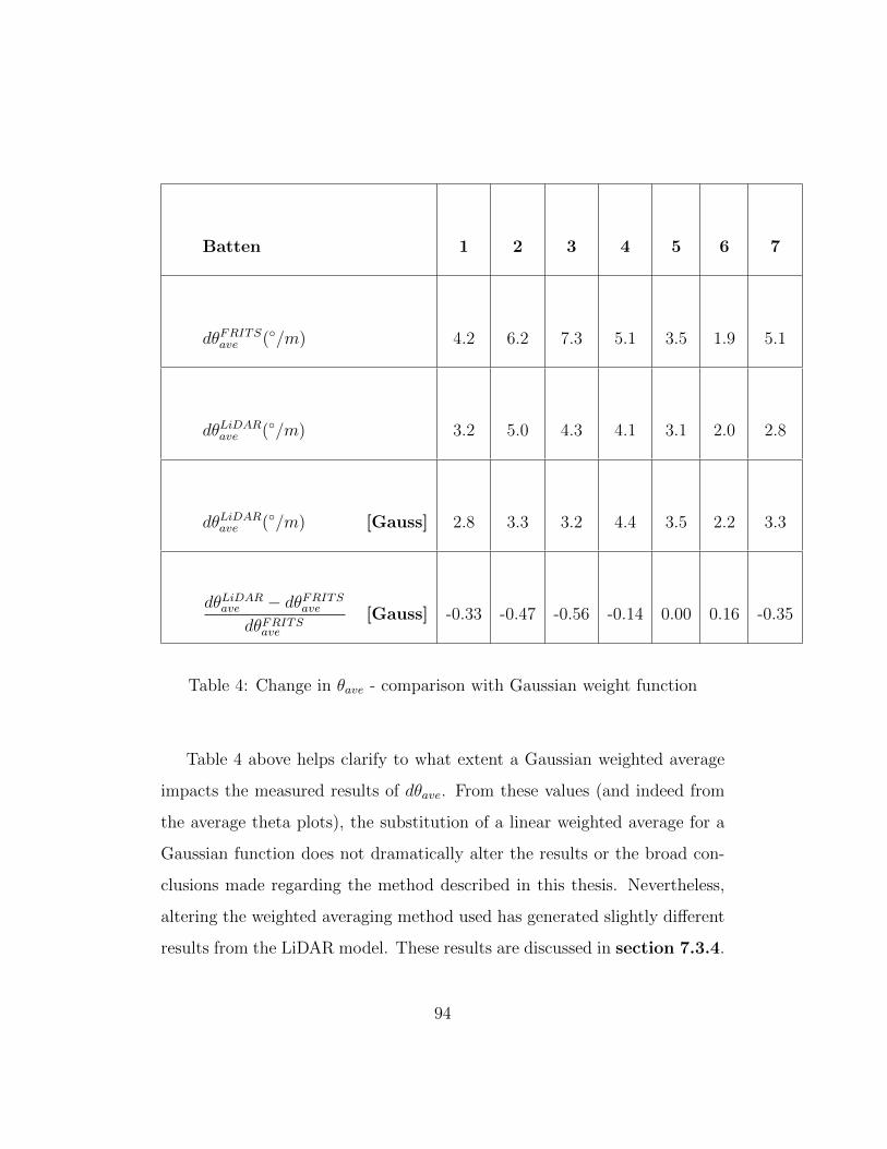
Batten 1 2 3 4 5 6 7
dθFRITSave (◦/m) 4.2 6.2 7.3 5.1 3.5 1.9 5.1
dθLiDARave (◦/m) 3.2 5.0 4.3 4.1 3.1 2.0 2.8
dθLiDARave (◦/m) [Gauss] 2.8 3.3 3.2 4.4 3.5 2.2 3.3
dθLiDARave − dθFRITS
ave
dθFRITSave
[Gauss] -0.33 -0.47 -0.56 -0.14 0.00 0.16 -0.35
Table 4: Change in θave - comparison with Gaussian weight function
Table 4 above helps clarify to what extent a Gaussian weighted average
impacts the measured results of dθave. From these values (and indeed from
the average theta plots), the substitution of a linear weighted average for a
Gaussian function does not dramatically alter the results or the broad con-
clusions made regarding the method described in this thesis. Nevertheless,
altering the weighted averaging method used has generated slightly different
results from the LiDAR model. These results are discussed in section 7.3.4.
94
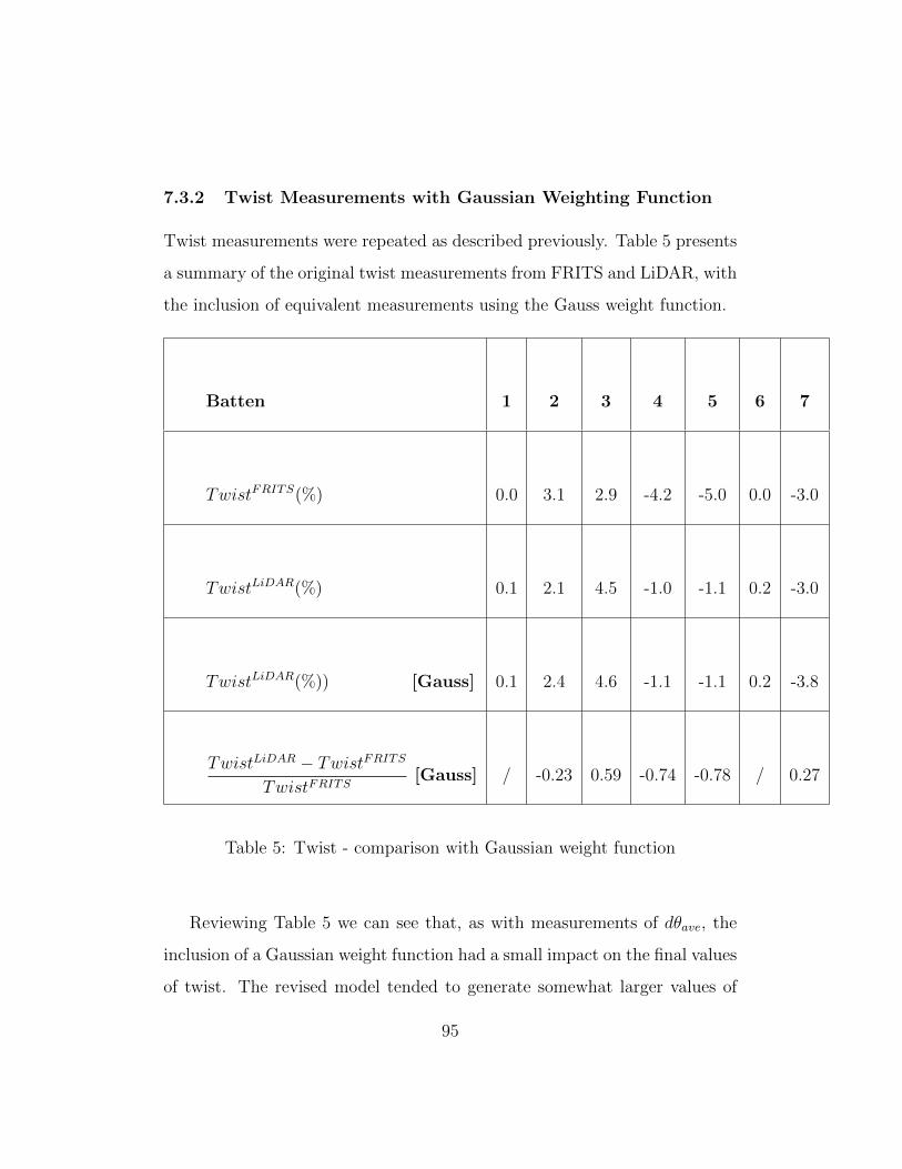
7.3.2 Twist Measurements with Gaussian Weighting Function
Twist measurements were repeated as described previously. Table 5 presents
a summary of the original twist measurements from FRITS and LiDAR, with
the inclusion of equivalent measurements using the Gauss weight function.
Batten 1 2 3 4 5 6 7
TwistFRITS(%) 0.0 3.1 2.9 -4.2 -5.0 0.0 -3.0
TwistLiDAR(%) 0.1 2.1 4.5 -1.0 -1.1 0.2 -3.0
TwistLiDAR(%)) [Gauss] 0.1 2.4 4.6 -1.1 -1.1 0.2 -3.8
TwistLiDAR − TwistFRITS
TwistFRITS[Gauss] / -0.23 0.59 -0.74 -0.78 / 0.27
Table 5: Twist - comparison with Gaussian weight function
Reviewing Table 5 we can see that, as with measurements of dθave, the
inclusion of a Gaussian weight function had a small impact on the final values
of twist. The revised model tended to generate somewhat larger values of
95
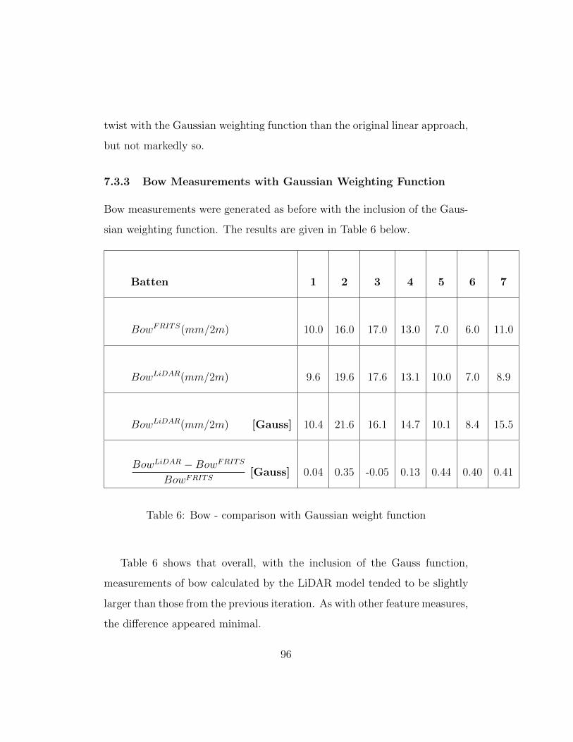
twist with the Gaussian weighting function than the original linear approach,
but not markedly so.
7.3.3 Bow Measurements with Gaussian Weighting Function
Bow measurements were generated as before with the inclusion of the Gaus-
sian weighting function. The results are given in Table 6 below.
Batten 1 2 3 4 5 6 7
BowFRITS(mm/2m) 10.0 16.0 17.0 13.0 7.0 6.0 11.0
BowLiDAR(mm/2m) 9.6 19.6 17.6 13.1 10.0 7.0 8.9
BowLiDAR(mm/2m) [Gauss] 10.4 21.6 16.1 14.7 10.1 8.4 15.5
BowLiDAR −BowFRITS
BowFRITS[Gauss] 0.04 0.35 -0.05 0.13 0.44 0.40 0.41
Table 6: Bow - comparison with Gaussian weight function
Table 6 shows that overall, with the inclusion of the Gauss function,
measurements of bow calculated by the LiDAR model tended to be slightly
larger than those from the previous iteration. As with other feature measures,
the difference appeared minimal.
96

7.3.4 Summary
This section has provided a useful insight into some of the underlying features
of the model presented in this thesis. Questioning some of the choices made
in constructing the original measurement model and assessing the impact of
alternative approaches aids in the overall evaluation of the model’s efficacy.
Given the focus of this thesis is to compare the LiDAR model with the
established standard of the FRITS method, reviewing Tables 4-6 we can see
that the inclusion of the Gauss function tended to broaden the gap between
FRITS measurements and LiDAR measurements.
In assessing the impact of using a Gaussian weighting function to average
orthogonal deviations within each neighbourhood, the size of the neighbour-
hoods themselves does not appear to be of great significance. Increasing
neighbourhood size ‘k’ from ten (the standard used throughout this thesis)
to fifty does not have any appreciable impact on the final distortion mea-
surements gained. Rather, the issue may be a question of scan resolution. In
their investigations into rendering point cloud samples, Alexa et al. discuss
the use of a Gaussian weighting function in the context of using dense and
often highly complex point clouds. These are far in advance of the medium-
range resolution scans used in this thesis. It may be that to achieve the
full benefits of an alternative weighting function, much denser, more detailed
scans would have to be carried out than were used in the experiments here.
In comparing the two averaging methods, while the differences in magni-
97
tude may appear numerically small, there is a potential that these differences
could impact on the final grading of a batten. For example, in the measure-
ment of bow in batten 2, both the FRITS and original LiDAR methods give
a value of bow less than 20mm/2m. In accordance with BS EN 14081-1, this
would meet the criteria for strength class C18 [BS EN 14081-1, 2005].
However, with the inclusion of the Gaussian weight function, the updated
LiDAR model gives a value of bow of 21.6mm/2m, i.e. slightly above the
threshold of maximum bow permissible for class C18. It is worth noting,
though, that the moisture content at which these battens were assessed was
lower than that at which distortion is typically measured. Considering this
low moisture content, a bow measurement of 21.6/2m could be considered
acceptable. It is interesting to note that across all three measurement meth-
ods (the FRITS, the LiDAR and the updated LiDAR) and across all three
feature measurements taken, batten 2 tended to be present one of the largest
degrees of distortion in the sample set used. Note also that the discrepan-
cies between FRITS measurement values and LiDAR measurement values for
batten 2 tended to be among the largest for measurements of dθave and bow
among the seven battens scanned.
It would appear then that in having greater disparities between orthogo-
nal deviations of reference surface point - or in other words, a greater degree
of distortion across the batten - the impact of the weighted averaging of those
deviations seems to be more apparent. Where there is little distortion to mea-
sure, in batten 6 for example, the differences between feature measurements
with a linear weighted averaging and a Gaussian equivalent seem to diminish.
98
With consideration of the above points, a thorough assessment of alternative
weighted averaging schemes would benefit from using higher resolution scans
than those used here. While far in excess of anything that can be achieved
with the FRITS, the LiDAR scans used for this project limited themselves to
a medium resolution level - relatively sparse in comparison to the higher reso-
lutions available. Further, the small sample size used here seemed to indicate
that the greatest impact of a change in weighted averaging appeared to be
present in those battens showing the greatest degree of distortion. Accord-
ingly, future experiments would benefit from focusing on battens showing
sizeable levels of distortion.
99

8 Discussion
Beyond the practical and quantitative comparisons between FRITS and Li-
DAR scanning, these investigations have generated a number of observations,
conclusions and recommendations regarding the broader issue of feature mea-
surement of timber battens and the existing measurement standards by which
battens are judged. Further, the experimentation with LiDAR scanning has
suggested new ways in which the approach could be exploited and developed
further in timber research, with particular reference to feature measurement.
8.1 Existing Standards
It was noted in section 1.3 that this research was in part motivated by the
deficiencies within standards BS EN1310:1997. These investigations have
highlighted some of these pre-existing issues and have given further credence,
if any were required, to the need for re-evaluation. The work into creating a
new feature measurement technique has generated specific recommendations
as to how the existing standards could be added to and improved.
From a geometric standpoint, the existing standards may appear to be ex-
haustive: the four measures of deviation (bow, spring, cup and twist) seem
to account for all the possible ways and directions in which a rectangular
batten may deviate. However, the standards limit themselves to using max-
imum values of deviation along single measurement lengths. On the other
hand, a measurement of the change in surface inclination (dθave), whereby
a greater proportion of the batten surface is covered, in both lateral and
100
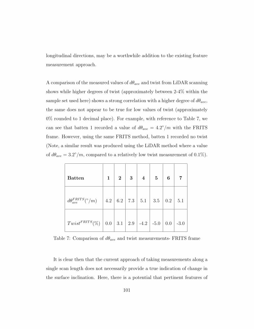
longitudinal directions, may be a worthwhile addition to the existing feature
measurement approach.
A comparison of the measured values of dθave and twist from LiDAR scanning
shows while higher degrees of twist (approximately between 2-4% within the
sample set used here) shows a strong correlation with a higher degree of dθave,
the same does not appear to be true for low values of twist (approximately
0% rounded to 1 decimal place). For example, with reference to Table 7, we
can see that batten 1 recorded a value of dθave = 4.2◦/m with the FRITS
frame. However, using the same FRITS method, batten 1 recorded no twist
(Note, a similar result was produced using the LiDAR method where a value
of dθave = 3.2◦/m, compared to a relatively low twist measurement of 0.1%).
Batten 1 2 3 4 5 6 7
dθFRITSave (◦/m) 4.2 6.2 7.3 5.1 3.5 0.2 5.1
TwistFRITS(%) 0.0 3.1 2.9 -4.2 -5.0 0.0 -3.0
Table 7: Comparison of dθave and twist measurements- FRITS frame
It is clear then that the current approach of taking measurements along a
single scan length does not necessarily provide a true indication of change in
the surface inclination. Here, there is a potential that pertinent features of
101

the batten surface are not begin captured. Instead, measurements that track
a wider surface area along the batten length, such as dθave, may provide a
more representative insight into changes of batten surface morphology and
could serve as an important addition to current standards.
Existing standards could be re-written then to adopt a more holistic ap-
proach to feature measurement. Standards could utilise measurements that
consider the batten more holistically and cover a larger area of the batten
surface, registering changes in deviation across the full length of the bat-
ten. With the introduction of LiDAR scanning technologies, this increase in
measurement sampling could be handled in a timely, efficient and accurate
way.
8.2 Outlook for the Use of LiDAR Scanning Within
Timber Research
Experimentation with the LiDAR scanner revealed a number of new areas of
potential interest from which future researches in feature measurement may
benefit. These ideas exploit the practical nature of LiDAR scanning in order
to further expand upon the existing FRITS frame approach.
With LiDAR scanning it would also be possible to scan the thinner, adjacent
edges of the batten to gain detailed distortion measurements not currently
possible using the FRITS. Spring, as defined in EN 1310:1997 could be mea-
sured easily using the same method described in this thesis, only with the
batten turned 90◦ such that its thin edge is presented to the scanner. From
102
this, plots of how the batten edge deviated from an undeformed datum could
be generated, giving a comprehensive measure of spring. Such detail would
not be possible with the current FRITS method. A batten resting on its
narrow edge within the frame presents a very limited area along which mea-
surements could be taken. Using the FRITS equipment, such an approach
allows for, at most, two scan lengths to be taken; in some cases only one
is possible. This incurs a great deal of interpolation between measurement
points and provides little insight into the actual morphology of the batten
edge.
Similarly, profiles of the end surface could be generated and analysed us-
ing LiDAR. Not only could this aid in the measuring of cup, for example,
they could also generate a comparison for how the batten profile changes
from one end of the batten to the other. End profiles like these cannot cur-
rently be replicated using the current method as the FRITS is limited to only
lengthwise scans.
In section 7.2.1 the potential for expanding the resolution of the reference
grid to give highly detailed measurements was touched upon. Measurements
of the batten ends could provide a avenue for further expansion of the Li-
DAR method as an accessible, smaller-scale alternative to industrial-sized
scanners. Currently, commercial laser scanners (such as the WoodEye Scan-
ner) can provide accurate, highly-detailed measurements, not just of batten
geometry but also of wood grain patterns. It is posited here that using a high
resolution LiDAR scan of the batten end at close range could, for example,
103
allow analysis of the annual growth rings or accurate positioning of the pith.
The problem would reduce down to an assessment of geometric information,
much like the solution presented in this thesis. The challenge, however, would
be in the successful management of significantly higher, more concentrated
point cloud data points. Nevertheless, the LiDAR method aims to provide
an accessible, practical comparative tool for timber analysis. Assessment of
annual growth rings is another possible area for expansion.
A natural progression of the LiDAR method is the use of three-dimensional
scans to describe the shape of the entire batten and not just one surface.
With the FRITS frame, measurements can be taken of both surfaces of a
batten and compared, the process is cumbersome and time consuming. To
scan two surfaces of a batten with the FRITS effectively doubles the work
load and proves an inefficient and often tedious process. However, multiple
LiDAR scans can be carried out with relative ease providing there is enough
room to manoeuvre around the batten. A minimum of two scans are required
to achieve a full 360◦ scan of a timber batten. This can be carried out within
five minutes on a medium scan resolution: far quicker and easier than the
FRITS. The process would require additional manipulation of the point cloud
data in order to map individual scans together to form a complete 3D model.
This is a standard requirement for many who work with LiDAR scanning
and such manipulation is easily provided for by the necessary software.
This research, and indeed the British Standards themselves, considered mea-
surements along one surface only and assumed the batten to be a rigid body,
104
with the deviation of one surface being matched by the surface underneath.
These may prove to be suitable assumptions in most cases; however, further
investigation is recommended to verify this. Although FRITS scans of op-
posing surfaces have been carried out by colleagues, again the necessarily
high interpolation required of the FRITS method may not be providing a
full picture of how the surface alters. Adopting the LiDAR scanner would
provide an efficient and more accurate alternative to this task.
105
9 Conclusion
For measurements of the change in surface inclination (dθave), the LiDAR
method developed in this project consistently compared well with the re-
sults obtained by the standard FRITS approach. Comparing final outputs
from the LiDAR with those of the FRITS, the LiDAR method differed from
the standard FRITS frame measurements by a mean value of −0.22◦/m
(σ = 0.17◦/m). In six out of the seven battens scanned, the LiDAR method
measured the change in surface inclination to be lower than that of the FRITS
frame.
Similarly, for measurements of the degree of twist along the leftmost edge, the
LiDAR method produced results comparable to those obtained by FRITS.
The LiDAR measurements differed from the FRITS standard by a mean
value of −0.26% (σ = 0.56%). Using LiDAR the degree of twist was found
to be higher than that found by FRITS in all but one of the seven battens.
In measuring bow, values extracted from LiDAR scans differed from those of
the FRITS method by an average value of 0.09mm/2m (σ = 0.2mm/2m).
In five out of the seven battens, the LiDAR method produced results for bow
that were larger than that obtained by FRITS.
The ongoing need for reassessment of existing standards was also highlighted
in this work. The investigations here have lead to the recommendation of an
expansion of BS EN 1310:1997 to include a standardised measure of surface
inclination (θave) in its list of distortion features. Currently, fixation on ‘rep-
106
resentative lengths’ to measure batten distortion do not paint an accurate
picture of batten morphology, nor are they broadly applicable to all battens.
Rather, the inclusion of a distortion feature more representative of the sur-
face as a whole would be a worthwhile addition to the feature measurement
standards. The increase in surface measurements required of this approach,
while cumbersome with the existing FRITS frame method, could be readily
and efficiently met by utilising LiDAR scanning technologies.
*
This thesis has helped introduce the use of LiDAR scanning to the field of
timber distortion measurement. It has served as a crucial proof of concept
for a heretofore untapped resource in a fertile area of timber research. It is
the hope of this work that the investigations detailed here have presented
LiDAR scanning as a viable, reliable new approach to distortion feature
measurement. Over reliance on a single measurement method will struggle
to provide new insights or improvements in distortion feature analysis, and
as such, the field may stagnate and fail to address the issues it currently
faces. The work in this report has confirmed that LiDAR scanning can
produce comparable results to the existing FRITS method, while being a far
more efficient, more practical approach. The technique also allows for further
development of the feature measurement process not currently capable with
existing methods. As such, the groundwork has been laid for LiDAR scanning
to become an approved and standard approach to measuring macroscopic
deformations of timber battens.
107
10 References
Alexa, M., Behr, J., Cohen-Or, D., Fleishman, S., Levin, D. and Silva, C.T.
(2003). Computing and Rendering Point Set Surface. IEEE TRANSAC-
TIONS ON VISUALIZATION AND COMPUTER GRAPHICS. 9, pp.3-15.
Almeida, G. and Hernandez, R.E. (2006). Changes in physical properties
of tropical and temperate hardwoods below and above the fibre saturation
point. Wood Science Technology. 40, pp.599-613.
Bergander, A. and Salmn, L. (2002). Cell wall properties and their effects
on the mechanical properties of fibres. Journal of Materials Science. 37,
pp.151-156.
Brandstrom, J. (2001). Micro- and ultrastructural aspects of Norway spruce
tracheids: a review. IAWA Journal. 22, pp.333-353.
British Standards Institute (1997). BS EN 1310:1997. Round and sawn
timber - Method of measurement of features. BSi.
British Standards Institute (2016). BS EN 14801-1. Timber structures
Strength graded structural timber with rectangular cross section Part 1:
General requirements. BSi.
Christensen, G.N. and Hergt H.F.A. (1969). Effect of previous history on
kinetics of sorption by wood cell walls. Journal of Polymer Science. 7,
108

pp.2427-2430.
Christensen, G.N. and Kelsey, K.E. (1959). The rate of sorption of water
vapour by wood. Holz Roh Werkst. 17, pp.178-188.
Curvescan [online]. (2016). Available from: http://microtec.eu/assets/products/
curvescan/Microtec-Curvescan-Optiside-1.pdf. [Accessed 21st August 2016].
Du, S. and Yamamoto, F. (2007). An Overview of the Biology of Reaction
Wood Formation. Journal of Integrative Plant Biology. 49(2), pp.131-143.
Eitelberger, J. (2011). A multiscale material description for wood below the
fibre saturation point with particular emphasis on wood-water interactions.
PhD thesis, Vienna University of Technology.
Ekevad, M. (2005). Twist of wood studs: dependence on spiral grain gradi-
ent. Journal of Wood Science. 51, pp.455461.
Engelund, E.T., Thygesen, L.G., Svensson, S and Hill, C.A.S. (2012). A crit-
ical discussion of the physics of wood-water interactions. In: COST Action
FP0802, 2008-2012: Experimental and computational micro-characterization
techniques in wood mechanics, 25 October 2012, Edinburgh.
Forestry Commission [online]. (2003). Available from:
http://www.forestry.gov.uk/fr/infd-4xgjc8.
109
[Accessed 4th January 2016].
Fransden, H.L. (2007). Selected constitutive model for simulating the hy-
gromechanical response of wood. PhD thesis, Aalborg University.
Goldeneye [online]. (2016). Available from: http://microtec.eu/en/catalogue/
products/goldeneye300/. [Accessed 21st August 2016].
Grohmann, R., Aleon, D., Knaggs, G., Lagana, R. and Baso, C. (2010).
COST Action E53 [online]. Available from:
http://www.coste53.net/index.php?Activities:Publications:Distortion of
Sawn Timber
[Accessed 2nd January 2016].
Hill, C.A.S., Norton, A.J. and Newman, G. (2010). Water vapour soprtion
properties of Sitka spruce determined using a dynamic vapour sorption ap-
paratus. Wood Science Technology. 44, pp.497-514.
Hill, C.A.S., Keating, B.A., Jaluladin, Z. and Mahrdt, E. (2012). A rhe-
ological description of the water vapour sorption kinetics behaviour of wood
invoking a model using a canonical assembly of Kelvin-Voigt elements and a
possible link with sorption hysteresis. Holzforschung. 66, pp.35-47.
Holland, C. and Reynolds, T. (2005) Timber grading and scanning. BRE
Digest. 492.
110

Johansson, M. (2006). Problem with distortion in timber Background and
explanations. In: COST Action E53 - International Workshop in Sopron, 9th
November 2006, Sopron. pp. 100-125.
Johansson, M. and Ormarsson, S. (2009). Influence of growth stresses and
material properties on distortion of sawn timber numerical investigation.
Annals of Forest Science. 66, pp.604-614.
Krabbenhft, K. (2003). Moisture transport in wood: A study of physical
mathematical models and their numerical implementation. PhD thesis, Tech-
nical University of Denmark.
Lukacevic M., Fussl J., Griessner M. and Eberhardsteiner, J. (2014). Per-
formance Assessment of a Numerical Simulation Tool for Wooden Boards
with Knots by Means of Full-Field Deformation Measurements. Strain. 50,
pp.301317.
Levin, D. (2004). Mesh-Independent Surface Interpolation. Geometric Mod-
elling for Scientific Visualization, Springer. pp.37-49.
Moore, A. (1991). Efficient Memory based Learning for Robot Control. PhD
thesis, University of Cambridge.
Neagu, R.C., Gamstedt, E.K., Bardage, S.L. and Lindstrm M. (2006). Ul-
111

trastructural features affecting mechanical properties of wood fibres. Wood
Material Science and Engineering. 1, pp.146-170.
New Zealand Timber Industry Federation [online]. (2007). Available from:
http://www.nzwood.co.nz/wp-content/uploads/2013/06/sawnmanufacture.pdf
[Accessed 4th January 2016].
O’Sullivan, A.C. (1997). Cellulose: the structure slowly unravels. Cellu-
lose. 4, pp.173-207.
Sandberg, D. (2005). Distortion and visible crack formation in green and
seasoned timber: influence of annual ring orientation in the cross section.
Holz als Roh- und Werkstoff. 63, pp.11-18.
Sandberg, K. and Salin, J. (2012). Liquid water absorption in dried Nor-
way spruce timber measured with CT scanning and viewed as a percolation
process. Wood Science Technology. 46, pp.207-219.
Seeling, U. and Merforth, C. (2000). FRITS - a new equipment to measure
distortion. Holz als Roh- und Werkstoff. 58, pp.338-339.
Stone, J.E. and Scallan, A.M. (1967). Effect of component removal upon
porous structure of cell wall of wood - 2. swelling in water and fibre satura-
tion point. Tappi. 50, pp.496-501.
Sun, S. and Salvaggio, C. (2013). Aerial 3D Building Detection and Mod-
112
elling From Airborne LiDAR Point Clouds. IEEE Journal of Selected Topics
in Applied Earth Observations and Remote Sensing. 6, pp.1440-1449.
Tagliasacchi, A. (2010). MathWorks [online]. Available from:
http://uk.mathworks.com/matlabcentral/fileexchange/21512-kd-tree-
for-matlab. [Accessed 26th November 2013].
Tiemann, H.D. (1906). Effect of Moisture upon the Strength and Stiffness
of Wood. 1st. ed. Harvard University: U.S. Dept. of Agriculture, Forest
Service.
Viscan [online]. (2016). Available from: http://microtec.eu/en/catalogue/
products/viscan. [Accessed 21st August 2016].
Watt, M.S., Kimberley, M.O., Harrington, J.J., Riddell, M.J.C., Cown, D.J.
and Moore, J.R. (2013). Differences in intra-tree variation in spiral grain an-
gle for radiata pine. New Zealand Journal of Forestry Science. 43, Article 12.
Weber, C., Hahmann, S. and Hagen, H. (2010). Sharp Feature Detection
in Point Clouds. In: IEEE International Conference on Shape Modelling
and Applications, 21-23 June 2010, Aix en Provence. pp. 175-186.
WoodEye [online]. (2016). Available from: http://woodeye.se/en/woodeye-
5/. [Accessed 2nd January 2016].
113