Bond Positions, Expectations, And The Yield Curve∗

Monika Piazzesi

Chicago GSB, FRB Minneapolis & NBER

Martin Schneider

NYU, FRB Minneapolis & NBER

February 2008

Abstract

This paper implements a structural model of the yield curve with data on nominal positions

and survey forecasts. Bond prices are characterized in terms of investors’ current portfolio

holdings as well as their subjective beliefs about future bond payoffs. Risk premia measured

by an econometrician vary because of changes in investors’ subjective risk premia, identified

from portfolios and subjective beliefs, but also because subjective beliefs differ from those of the

econometrician. The main result is that investors’ systematic forecast errors are an important

source of business-cycle variation in measured risk premia. By contrast, subjective risk premia

move less and more slowly over time.

∗Preliminary and incomplete. Comments welcome! We thank Ken Froot for sharing the Goldsmith-Nagan surveydata with us, and the NSF for financial support to purchase the Bluechip survey data. We also thank Andy Atkeson,Jon Faust, Bing Han, Lars Hansen, Narayana Kocherlakota, Glenn Rudebusch, Ken Singleton, Dimitri Vayanos,seminar participants at the San Francisco Federal Reserve Bank, UT Austin and conference participants at theAtlanta Federal Reserve Bank, ECB “Risk Premia” conference, 2007 Nemmers Conference at Northwestern University,“Conference on the Interaction Between Bond Markets and the Macro-economy” at UCLA and the Summer 2007Vienna conference. Email addresses: piazzesi@uchicago.edu, martin.schneider@nyu.edu. The views expressed hereinare those of the authors and not necessarily those of the Federal Reserve Bank of Minneapolis or the Federal ReserveSystem.

1

I Introduction

Asset pricing theory says that the price of an asset is equal to the expected present value of its

payoff, less a risk premium. Structural models relate the risk premium to the covariance between

the asset payoff and investors’ marginal utility. Quantitative evaluation of asset pricing models

thus requires measuring investors’ expectations of both asset payoffs and marginal utility. The

standard approach is to estimate a time series model for these variables, and then invoke rational

expectations to argue that investors’ beliefs conform with the time series model. The standard

approach has led to a number of asset pricing puzzles. For bonds, the puzzle is that long bond

prices are much more volatile than expected long bond payoffs, and that returns on long bonds

appear predictable.

This paper considers a model of bond returns without assuming rational expectations. Instead,

we use survey forecasts and data on investor asset positions to infer investors’ subjective distribution

of asset payoffs and marginal utility. The basic asset pricing equation—price equals expected payoff

plus risk adjustment—holds in our model, even though investors do not have rational expectations.

Consider the price P (n)t of a zero-coupon bond of maturity n. In particular, there is a pricing kernel

M∗, such that

P(n)t =

1

RtE∗t P

(n−1)t+1 + cov∗t

³M∗

t+1, P(n−1)t+1

´,

where Rt is the riskless rate. The expected payoff from a zero coupon bond next period is the

expected price next period, when the bond will have maturity n−1. The risk premium depends onhow that price covaries withM∗. The key difference to the standard approach is that both moments

are computed under a subjective probability distribution, indicated by an asterisk. This subjective

distribution is estimated using survey data, and can be different from the objective distribution

implied by our own time series model.

Asset pricing puzzles arise because observed bond prices are more volatile than present values

of expected payoffs computed under an objective distribution used by the researcher, EtP(n−1)t+1 say.

To see how our model speaks to the puzzles, rewrite the equilibrium price as

(1) P(n)t =

1

RtEtP

(n−1)t+1 + cov∗t

³M∗

t+1, P(n−1)t+1

´+1

Rt

³E∗t P

(n−1)t+1 −EtP

(n−1)t+1

´.

2

The equilibrium price can deviate from objective expected payoffs not only because of (subjective)

risk premia, but also because subjective and objective expectations differ. Under the rational

expectations approach, the second effect is assumed away. Structural models then fail because they

cannot generate enough time variation in risk premia to account for all price volatility in excess of

volatility in (objectively) expected payoffs.

This paper explores asset pricing under subjective expectations in three steps. First, we doc-

ument properties of subjective expectations of interest rates using survey data over the last four

decades. Here we show that the last term in (1) is not zero, and moves systematically over the

business cycle. Second, we estimate a reduced form model that describes jointly the distribution of

interest rates and inflation and investors’ subjective beliefs about these variables. Since we impose

the absence of arbitrage opportunities in bond markets, we can recover a subjective pricing kernel

M∗ implied by survey forecasts. This allows us to quantify the contribution of forecast errors to

the excess volatility and predictability of bond prices. Third, we derive subjective risk premia in a

representative agent model, where M∗ reflects the investor’s marginal rate of substitution.

The first step combines evidence from the Blue Chip survey, available since 1982, as well as

its precursor, the Goldsmith-Nagan survey, available since 1970. We establish two stylized facts.

First, there are systematic differences in subjective and objective interest-rate expectations, and

hence bond prices and excess returns on bonds. We compare expected excess returns on bonds

implied by predictability regressions that are common in the literature to expected excess returns

on bonds perceived by the median survey investor. We find survey expected excess returns to be

both smaller on average and less countercyclical than conventional measures of expected excess

returns. In particular, conventionally measured expected returns appear much higher than survey

expected excess returns during and after recessions.

The second stylized fact is that there are systematic biases in survey forecasts. In particular,

with hindsight, survey forecasters do a bad job forecasting mean reversion in yield spreads after

recessions This finding says that the first stylized fact is not driven by our choice of a particular, and

thus perhaps inadequate, objective model. To the contrary, the better the forecasting performance

of the time series model used to construct objective forecasts, the larger will be the difference

between those forecasts and survey forecasts.

3

In the second part of the paper, we estimate a reduced form model using interest rate data

for many different maturities as well as forecast data for different maturities and forecast hori-

zons. To write down a parsimonious model that nevertheless uses all the information we have, we

employ techniques familiar from the affine term structure literature. There, actual interest rates

are represented as conditional expectations under a “risk neutral probability”, which are in turn

affine functions of a small number of state variables. The Radon-Nikodym derivative of the risk

neutral probability with respect to the objective probability that governs the evolution of the state

variables then captures risk premia. Our exercise also represents subjective forecasts as conditional

expectations under a subjective probability, again written as an affine function of the state vari-

ables. The Radon-Nikodym derivative of this subjective probability with respect to the objective

probability then captures forecast biases, and can be identified from survey data.

The main result from the estimated reduced form model is that survey forecasters perceive both

the level and the slope of the yield curve to be more persistent than they are under an objective

statistical model. For example, in the early 1980s when the level of the yield curve was high,

survey forecasters expected all interest rates to remain high whereas statistical models predicted

faster reversion to the mean. In addition, at the end of recessions when the slope of the yield curve

was high, survey forecasters believed spreads on long bonds to remain high, whereas statistical

models predicted faster mean reversion in yield spreads.

By equation (1), both biases have important implications for the difference between objective

and subjective risk premia. First, both biases imply that survey forecasters predict lower bond

prices, and hence lower excess returns than statistical models when either the level or the slope of

the yield curve is high. However, times of high level or high slope are precisely the times when

objective premia are high. This explains why we find subjective premia that are significantly less

volatile than objective premia: the volatility of 1-year holding premia is reduced by 40%-60%,

depending on the maturity of the bond.

A second implication is that subjective and objective premia have different qualitative proper-

ties. For long bonds (such as a 10 year bond), yields move relatively more with the slope of the

yield curve as opposed with the level. As a result, the bias in spread forecasts is more important.

This goes along with the fact that objective premia on long bonds also move more with the slope of

4

the yield curve. Subjective premia of long bond are thus not only less volatile, but also much less

cyclical. The lesson we draw for the structural modelling of long bonds is that the puzzle is less

that premia are cyclical, but rather that they were much higher in the early 1980s than at other

times. For medium term bonds (such as a two year bond), which relatively more with the level of

the yield curve, the bias in level forecasts is more important. It implies that subjective premia are

somewhat lower than objective premia in the 1980s, but both premia share an important cyclical

component.

The third part of the paper proposes a new way to empirically evaluate a structural asset pricing

model, using data on not only survey expectations, but also investor asset positions. The theoretical

model is standard: we consider a group of investors who share the same Epstein-Zin preferences.

We assume that these investors hold the same subjective beliefs — provided by our reduced form

model — about future asset payoffs. To evaluate the model quantitatively, we work out investors’

savings and portfolio choice problem given the beliefs to derive asset demand, for every period in

our sample. We then find prices that make asset demand equal to investors’ observed asset holdings

in the data. We thus arrive at a sequence of model-implied bond prices of the same length as the

sample. The model is “successful” if the sequence of model-implied prices is close to actual prices.

Since there is a large variety of nominal instruments, an investor’s “bond position” is in principle

a high-dimensional object. To address this issue, we use the subjective term-structure model to

replicate positions in many common nominal instruments by portfolios that consist of only three zero

coupon bonds. Three bonds work because a two-factor model does a good job describing quarterly

movements in the nominal term structure. The replicating portfolios shed light on properties of

bonds outstanding in the US credit market. One interesting fact is that the relative supply of longer

bonds declined before 1980, as interest rate spreads were falling, but saw a dramatic increase in

the 1980s, a time when spreads were extraordinarily high.

We illustrate our asset pricing approach by presenting an exercise where investors are assumed to

be “rentiers”, that is, they hold only bonds. Rentiers’ bond portfolios are taken to be proportional

to those of the aggregate US household sector, and we choose preference parameters to best match

the mean yield curve. This leads us to consider relatively patient investors with low risk aversion.

Our model then allows a decomposition of “objective” risk premia as measured under the objective

5

statistical model of yields into their three sources of time variation. We find that subjective risk

premia are small and vary only at low frequencies. This is because both measured bond positions,

and the hedging demand for long bonds under investors’ subjective belief move slowly over time.

In contrast, the difference in subjective and objective forecasts is a source of large time variation

in risk premia at business cycle frequencies.

We build on a small literature which has shown that measuring subjective beliefs via surveys can

help understand asset pricing puzzles. Froot (1989) argued that evidence against the expectations

hypothesis of the term structure might be due to the failure of the (auxiliary) rational expectations

assumption imposed in the tests rather than to failures of the expectations hypothesis itself. He

used the Goldsmith-Nagan survey to measure interest rate forecasts and found that the failure

of the expectations hypothesis for long bonds can be attributed to expectational errors. The

findings from our reduced form model confirm Froot’s results while including the BlueChip data

set that allows for a longer sample as well as more forecast horizons and maturities. Moreover, our

estimation jointly uses all data and recovers and characterizes the entire subjective kernel M∗.1

Several authors have explored the role of expectational errors in foreign exchange markets. Frankel

and Froot (1989) show that much of the forward discount can be attributed to expectational errors.

Gourinchas and Tornell (2004) use survey data to show that deviations from rational expectations

can rationalize the forward premium and delayed overshooting puzzles. Bacchetta, Mertens and

van Wincoop (2008) study expectational errors across a large number of asset markets.

The rest of the paper is structured as follows. Section II introduces the modelling framework.

Section III documents properties of survey forecasts. Section IV describes estimation results for the

reduced form model. Section V explains how we replicate nominal position by simple portfolios.

Section VI reports results from the structural model.

1Kim and Orphanides (2007) estimate a reduced-form term structure model using data on both interest rates andinterest rate forecasts. They show that incorporating survey forecasts into the estimation sharpens the estimates ofrisk premia in small samples. In our language, they obtain more precise estimates of “objective premia”; they arenot interested in the properties of subjective risk premia for structural modelling.

6

II Setup

Investors have access to two types of assets. Bonds are nominal instruments that promise dollar-

denominated payoffs in the future. In particular, there is a one period bond — from now on, the

short bond — that pays off one dollar at date t+1; it trades at date t at a price e−it . Its real payoff

is e−πt+1 , where πt is (log) inflation.2 In addition to short bonds, there are long zero-coupon bonds

for all maturities; a bond of maturity n trades at log price p(n)t at date t and pays one dollar at

date t+n. The log excess return over the short bond from date t to date t+1 on an n-period bond

is defined as x(n)t+1 = p(n−1)t+1 − p

(n)t − it. In some of our exercises, we also allow investors to trade a

residual asset, which stands in for all assets other than bonds. The log real return from date t to

date t+ 1 is rrest+1, so that its excess return over the short bond is xrest+1 = rrest+1 − it − πt+1.

A. Reduced form model

We describe uncertainty about future returns with a state space system. The basic idea is to start

from an objective probability P , provided by a system with returns and other variables that fits

the data well from our (the modeler’s) perspective. A second step then uses survey expectations

to estimate the state space system under the investor’s subjective probability, denoted P ∗.

The state space system is for an S-vector of observables ht which contains all variables that are

needed to describe the statistical properties of nominal returns and inflation (so that investors can

compute real returns.) Under the objective probability P , the state space system is

ht = μh + ηhst−1 + et(2)

st = φsst−1 + σset,

where st and et are S-vectors of state variables and i.i.d. zero-mean normal shocks with Eete>t = Ω,

respectively. The first component of ht is always the short interest rate i(1)t and the first state

2This is a simple way to capture that the short (1 period) bond is denominated in dollars. To see why, considera nominal bond which costs P (1)

t dollars today and pays of $1 tomorrow, or 1/pct+1 units of numeraire consumption.Now consider a portfolio of pct nominal bonds. The price of the portfolio is P

(1)t units of consumption and its payoff

is pct/pct+1 = 1/πt+1 units of consumption tomorrow. The model thus determines the price P

(1)t of a nominal bond in

$.

7

Figure 1: Relationship between the different probability measures

variable is the demeaned short interest rate, that is, st,1 = i(1)t − μ1.

From objective to subjective probability

We assume that investors’ beliefs are also described by the state space system, but with different

coefficients. To define investors’ subjective beliefs, we represent the Radon-Nikodym derivative of

investors’ subjective belief P ∗ with respect to the objective probability P by a stochastic process

ξ∗t , with ξ∗1 = 1 and

(3)ξ∗t+1ξ∗t

= exp

µ−12κ>t Ωκt − κ>t et+1

¶.

Since et is i.i.d. mean-zero normal with variance Ω under the objective probability P , ξ∗t is a

martingale under P . Since et is the error in forecasting ht, the process κt can be interpreted as

investors’ bias in their forecast of ht. The forecast bias is affine in state variables, that is

κt = k0 + k1st.

Standard calculations now deliver that e∗t = et + Ωκt is i.i.d. mean-zero normal with variance

matrix Ω under the investors’ belief P ∗, so that the dynamics of ht under P ∗ can be represented

8

by

ht = μh −Ωk0 + (ηh −Ωk1)st−1 + e∗t := μ∗h + η∗hst−1 + e∗t(4)

st = −σsΩk0 + (φs − σsΩk1)st−1 + σse∗t := μ∗s + φ∗sst−1 + σse

∗t

The vector k0 thus affects investors’ subjective mean of ht and also the state variables st, whereas

the matrix k1 determines how their forecasts of h deviate from the objective forecasts as a function

of the state st.

Other bond prices

Our description of subjective beliefs needs to deal with the fact that we allow investors to invest

in bonds of all maturities. As a consequence, the number of bond returns (and state variables) in the

state space system (4) can become very large. By assuming the absence of arbitrage opportunities

in bond markets, we can obtain a more parsimonious system. Another advantage of this approach

is that a small number of bonds will be enough to span bond markets, which makes the portfolio

choice problem of investors manageable.

An implication of the no-arbitrage assumption is that there exists a “risk neutral” probability

Qunder which bond prices are discounted present values of bond payoffs. In particular, the prices

P (n) of zero-coupon bonds with maturity n satisfy the recursion

P(n)t = e−itEQ

t

hP(n−1)t+1

i

with terminal condition P(0)t = 1.

As illustrated in Figure 1, we specify the Radon-Nikodym derivative ξQt of the risk neutral

probability Q with respect to the objective probability P by ξQ1 = 1 and

ξQt+1

ξQt= exp

µ−12λ>t Ωλt − λ>t et+1

¶,

where λt is an S-vector which contains the “market prices of risk” associated with innovations et+1.

9

We assume that risk premia are linear in the state vector, that is,

λt = l0 + l1st,

for some S × 1 vector l0 and some S × S matrix l1. With this specification, eQt = et + Ωλt is an

i.i.d. zero-mean normal innovation under Q. The state vector dynamics under Q are

st = −σsΩl0 + (φs − σsΩl1)st−1 + σseQt := μQs + φQs st−1 + σse

Qt .

We select a subset of the state variables as term-structure factors ft = ηfst using the selection

matrix η = [IF×F 0F×S−F ] . The advantage of this approach is that we can describe the time-t

price for a bond with any maturity n as an exponential-linear function of only F factors. Standard

calculations deliver that the price is

(5) P(n)t = exp

³An +B>n ft

´

where An is a scalar and Bn is an F × 1 vector of coefficients that depend on maturity n.

Given these formulas for bond prices, interest rates i(n)t = − lnP (n)t /n are also linear functions of

the factors with the coefficients an = −An/n and bn = −Bn/n. Moreover, the objective expectation

of the excess (log) return on an n-period bond is

(6) Et

hx(n)t+1

i+1

2V art [xt+1] = B>n−1σfΩλt.

This affine function in the state vector has a constant which depends on the parameter l0 and a

slope coefficient which is driven by l1. The expression shows that the expectations hypothesis holds

under the objective probability if l1 = 0.

Investors have beliefs P ∗ rather than P , and so their subjective market prices of risk are not

equal to λt. Instead, their subjective market price of risk process is λ∗t = λt − κt, so that the bond

prices computed earlier are also risk-adjusted present discounted values of bond payoffs under the

10

subjective belief P ∗:

P(n)t = e−itEQ

t

hP(n−1)t+1

i= e−itE∗t

∙exp

µ−12λ∗>t Ωλ

∗t − λ∗>t et+1

¶P(n−1)t+1

¸.

Investors have subjective excess (log) returns expectations

E∗thx(n)t+1

i+1

2V ar∗t [xt+1] = B>n−1σfΩλ

∗t ,

which depend on the parameters of the subjective market price of risk process. The expectations

hypothesis holds under their beliefs provided that l∗1 = 0.

B. Structural model

A large number of identical investors live forever. Their preferences over consumption plans are

represented by Epstein-Zin utility with unitary intertemporal elasticity of substitution. The utility

ut of a consumption plan (Cτ )∞τ=t solves

(7) ut = (1− β) logCt + β logE∗the(1−γ)ut+1

i 11−γ

,

where E∗ denotes the expectation operator based on the subjective probability measure P ∗. In-

vestors’ ranking of certain consumption streams is thus given by discounted logarithmic utility.

At the same time, their attitude towards atemporal lotteries is determined by the risk aversion

coefficient γ. We focus below on the case γ > 1, which implies an aversion to persistent risks (as

discussed in Piazzesi and Schneider 2006).

Investors start a trading period t with initial wealth W t. They decide how to split this initial

wealth into consumption as well as investment in F + 2 assets: the residual asset, F long bonds,

and the short bond. These F +1 bonds are enough to span bond markets, because bond prices (5)

depend on F factors. We collect the log nominal prices of the F long bonds — which we refer to as

spanning bonds — at date t in a vector pt, and we collect their log nominal payoffs3 at date t+1 in

3This notation is convenient to accomodate the fact that the maturity of zero-coupon bonds changes from onedate to the next. For example, assume that there is only one long bond, of maturity n, and let i(n)t denote its yield

11

a vector p+1t+1. The log excess returns over the short bond from date t to date t+ 1 on these bonds

can thus be written bxt+1 = p+1t+1 − pt − it.

We denote by ωrest the portfolio weight on the residual asset (that is, the fraction of savings in-

vested in that asset), and we collect the portfolio weights on the spanning bonds in an F -dimensional

vector bωt, so that 1−ωrest − ι>bωt is the weight on the short bond, where ι denotes a vector of ones.Therefore, the one-period return on wealth from date t to date t+1 is RW

t+1 =PF+2

i=1 ωit exp¡rit+1

¢,

where ωit is the date-t portfolio weight on asset i and rit+1 is its log real return from t to t+1. The

household’s sequence of budget constraints can then be written as4

W τ+1 = Rwτ+1

¡W τ − Cτ

¢,

Rwτ+1 =

³1 + ωresτ

¡exp

¡xresτ+1

¢− 1¢+ bω>τ (exp (xτ+1)− ι)´exp (iτ − πτ+1) ; τ ≥ t.(8)

The household problem at date t is to maximize utility (7) subject to (8), given initial wealth W t

as well as subjective beliefs about returns. These beliefs are based on current bond prices pt, the

current short rate it, as well as the conditional distribution of the vector¡rresτ , iτ , πτ , pτ , p

+1τ

¢τ>t

,

that is, the return on the residual asset, the short interest rate, the inflation rate and the prices

and payoffs on the long spanning bonds. We denote this conditional distribution by P ∗t .

We now relate bond prices to positions and subjective expectations using investors’ optimal

policy functions. Since preferences are homothetic and all assets are tradable, optimal consumption

and investment plans are proportional to initial wealth. The optimal portfolio weights on long bonds

and the residual asset thus depend only on subjective beliefs about returns and can be written

as bωt (it, pt, P ∗t ) and ωrest (it, pt, P∗t ), respectively. Moreover, with an intertemporal elasticity of

substitution of one, the optimal consumption rule is Ct = (1− β)W t. Now suppose we observe

investors’ bond positions: we write Bt for the total dollar amount invested in bonds at date t, and

we collect investors’ holdings of the F long bonds in the vector bBt.

We perform two types of exercises. Consider first a class of investors who invest only in bonds;

there is no residual asset. These “rentier” investors have wealth Bt and so their portfolio weights

to maturity. The long bond trades at date t at a log price pt = −ni(n)t , and it promises a log payoff at date t+ 1 ofp+1t+1 = − (n− 1) i(n−1)t+1 .

4Here exp (xt) is an F -vector with the jth element equal to exp (xt,j).

12

on long bonds are

(9) bωt (it, pt, P ∗t ) = Bt

Bt.

These equations can be solved for long bond prices pt as a function of the short rate it, bond

positions (Bt, Bt) and subjective expectations P ∗t . We can thus characterize yield spreads in terms

of these variables.

Second, suppose there is a residual asset. Since investors’ wealth equals their savingsW t−Ct =

βW t =β1−βCt, we must have

bωt (it, pt, P ∗t ) =1− β

β

Bt

Ct,(10)

ωrest (it, pt, P∗t ) = 1− 1− β

β

Bt

Ct.

These equations can be solved for long bond prices pt and the short rate it, as a function of bond

positions (Bt, Bt), consumption Ct and expectations P ∗t . This characterizes both short and long

yields in terms of positions and subjective expectations.

III Preliminary evidence about subjective beliefs

We measure subjective expectations of interest rates with survey data from two sources. Both

sources conduct comparable surveys that ask approximately 40 financial market professionals for

their interest-rate expectations at the end of each quarter and record the median survey response.

Our first source are the Goldsmith-Nagan surveys that were started in mid-1969 and continued until

the end of 1986. These surveys ask participants about their one-quarter ahead and two-quarter

ahead expectations of various interest rates, including the 3-month Treasury bill, the 12-month

Treasury bill rate, and a mortgage rate. Our second source are Bluechip Financial Forecasts, a

survey that was started in 1983 and continues until today. This survey asks participants for a

wider range of expectation horizons (from one to six quarters ahead) and about a larger set of

interest rates. The most recent surveys always include 3-month, 6-month and 1-year Treasury bills,

13

the 2-year, 5-year, 10-year and 30-year Treasury bonds, and a mortgage rate.5

To measure objective interest-rate expectations, we estimate unrestricted VAR dynamics for

a vector of interest rates with quarterly data over the sample 1964:1-2007:4 and compute their

implied forecasts. Later, in Section IV, we will impose more structure on the VAR by assuming

the absence of arbitrage and using a lower number of variables in the VAR, and thereby check the

robustness of the empirical findings we document here. The vector of interest rates Y includes

the 1-year, 2-year, 3-year, 4-year, 5-year, 10-year and 20-year zero-coupon yields. We use data on

nominal zero-coupon bond yields with longer maturities from the McCulloch file available from the

website http://www.econ.ohio-state.edu/jhm/ts/mcckwon/mccull.htm. The sample for these data

is 1952:2 - 1990:4. We augment these data with the new Gurkaynak, Sack, and Wright (2006) data.

We compute the forecasts by running OLS directly on the system Yt+h = μ + φYt+ εt+h, so that

we can compute the h-horizon forecast simply as μ+ φYt.

Deviations of subjective expectations from objective expectations of interest rates have conse-

quences for expected excess returns on bonds. We write the (log) excess return on an n-period bond

for a h-period holding period as the log-return from t to t+h on the bond in excess of the h-period

interest rate, x(n,h)t+h = p(n−h)t+h − p

(n)t − hi

(h)t . The objective expectation E of an excess returns can

be decomposed as follows:

Et

hx(n,h)t+h

i| z = E∗t

hx(n,h)t+h

i+Et

hp(n−h)t+h

i−E∗t

hp(n−h)t+h

i(11)

= E∗thx(n,h)t+h

i| z +(n− h)

³E∗thi(n−h)t+h

i−Et

hi(n−h)t+h

i´| z

objective premium = subjective premium + subj. - obj. interest-rate expectation

This expression shows that, if subjective expectations E∗ of interest rates deviate from their objec-

tive expectations E, the objective premium is different from the subjective premium. In particular,

if the difference between objective and subjective beliefs changes in systematic ways over time, the

objective premium may change over time even if the subjective premium is constant.

We can evaluate equation (11) based on our survey measures of subjective interest-rate ex-5The survey questions ask for constant-maturity Treasury yield expectations. To construct zero-coupon yield

expectations implied by the surveys, we use the following approximation. We compute the expected change in then-year constant-maturity yield. We then add the expected change to the current n-year zero-coupon yield.

14

pectations E∗thi(n−h)t+h

iand the VAR measures of objective expectations Et

hi(n−h)t+h

ifor different

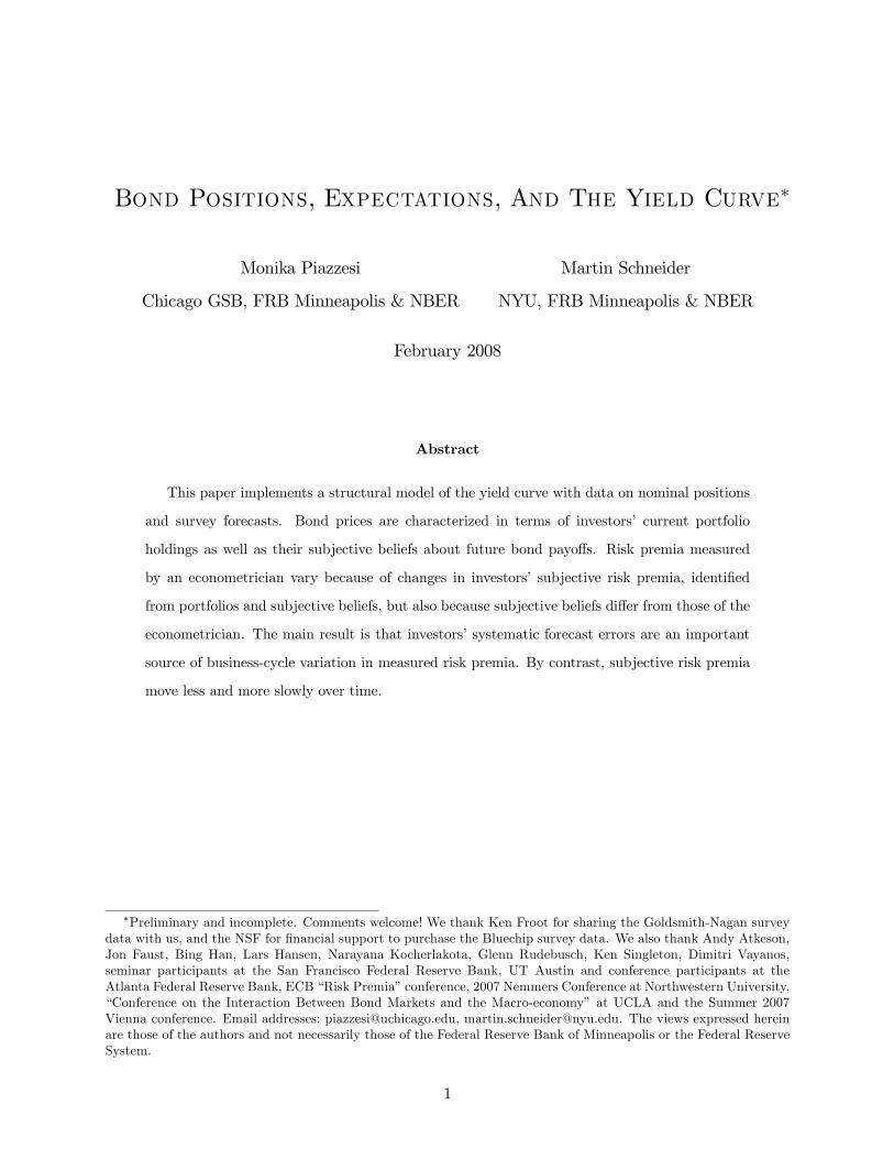
maturities n and different horizons h. Figure 2 plots the left-hand side of equation (11), expected

excess returns under objective beliefs as a black line, and the second term on the right-hand side

of the equation, the difference between subjective and objective interest-rate expectations, as a

gray line. For the short post-1983 sample for which we have Bluechip data, we have data for many

maturities n and many forecasting horizons h. The lower two panels of Figure 2 use maturities n =

3 years and 11 years and a horizon of h = 1 year, so that we deal with expectations of the n − h

= 2 year and 10 year interest rate. These combinations of n and h are in the Bluechip survey, and

the VAR includes these two maturities as well so that the computation of objective expectations is

easy.

For the long post-1970 sample, we need to combine data from the Goldsmith-Nagan and

Bluechip surveys. The upper left panel shows the n = 1.5 year bond and h = 6 month hold-

ing period. from the estimated VAR (which includes the n−h = 1 year yield.) This works, becauseboth surveys include the n−h = 1 year interest rate and a h = 6-month horizon. The VAR deliversan objective 6-month ahead expectation of the 1-year interest rate. For long bonds, we do not have

consistent survey data over this long sample. To get a rough idea of long-rate expectations during

the Great Inflation, we take the Goldsmith-Nagan data on expected mortgage-rate changes and the

Bluechip data on expected 30-year Treasury-yield over the next h = 2 quarters and add them to

the current 20-year zero-coupon yield. The VAR produces a h = 2 quarter ahead forecast of the

20-year yield.

Figure 2 also shows NBER recessions as shaded areas. The plots indicate that expected excess

returns under objective beliefs and the difference between subjective and objective interest-rate

expectations have common business-cycle movements. The patterns appear more clearly in the

lower panels which use longer (1 year) horizons. This is not surprising in light of the existing

predictability literature which documents that expected excess returns on bonds and other assets

are countercyclical when we look at longer holding periods, such as one year (e.g., Cochrane and

Piazzesi 2005.) In particular, expected excess returns are high right after recession troughs. The

lower panels show indeed high values for both series around and after the 1991 and 2001 recessions.

The series are also high in 1984 and 1996, which are years of slower growth (as indicated, for

15

1970 1980 1990 2000

-5

0

5

10

Long sample, n = 1.5 years, h = 6 monthspe

rcen

t, an

nual

ized

1970 1980 1990 2000

-60

-40

-20

0

20

Long sample, n = 20.5 years, h = 6 months

1985 1990 1995 2000 2005

-2

-1

0

1

2

3

4

5Short sample, n = 3 years, h = 1 year

perc

ent

1985 1990 1995 2000 2005-10

-5

0

5

10

15

Short sample, n = 11 years, h = 1 year

Figure 2: Each panel shows objective expectations of excess returns in black (the left-hand sideof equation (11)) and the difference between subjective and objective interest-rate expectations ingray (the second term on the right-hand side of the equation) for the indicated bond maturity nand holding period/forecast horizon h. Shaded areas indicate NBER recessions. The numbers areannualized and in percent. The upper panels show data over a longer sample than the lower panels.

example, by employment numbers) although they were not classified as recessions.

For shorter holding periods, the patterns are also there in the data but they are much weaker.

However, the upper panels show additional recessions where similar patterns appear. For example,

the two series in both panels are high in the 1970, 1974, 1980 and 1982 recessions or shortly

afterwards. (As we can see in the upper panels, expected excess returns for short holding periods

are large when annualized. Of course, the risk involved in these investment strategies is high, and

16

so they are not necessarily attractive.)

Table 1 shows summary statistics of subjective beliefs measured from surveys. During the short

Bluechip sample, the average difference between realized interest rates and their one-quarter ahead

subjective expectation is negative for short maturities and close to zero, or slightly positive for

longer maturities. The average forecast error is −15 basis points for the 3-quarter interest rateand −45 basis points for the 6-quarter interest rates. These two mean errors are the only onesthat are statistically significant, considering the sample size of 98 quarters (which means that the

ratio of mean to standard deviation needs to be multiplied by roughly 10 to arrive at the relevant

t-statistic.) There is stronger evidence of bias at the 1-year horizon, where on average subjective

interest-rate expectations are above subsequent realizations for all maturities. During the long

combined Goldsmith-Nagan and Bluechip sample, the average 2-quarter ahead forecast errors are

−54 and −27 basis points for the 3-month and 1-year yields. The average 1-quarter forecast errorsare also negative for these maturities. The column for the 30 year yield in Table 1 includes the

average forecast errors for the constructed long bond. The roughly 10 bp errors for this long interest

rate needs to be viewed with some caution due to how we constructed the survey series for this

bond (as explained earlier.)

The upward bias in subjective expectations may partly explain why we observe positive average

excess returns on bonds. The right-hand side of equation (11) shows why: if objective expectations

are unbiased, then E∗t i(n−h)t+h > Eti

(n−h)t+h on average, which raises the value of the left-hand side of the

equation. The magnitude of the bias is also economically significant. For example, the −56 basis-point bias in subjective expectations of the 1-year interest rate contributes 56 basis points to the

objective premium on the 2-year bond. For higher maturities, we need to multiply the subjective

bias by n − 1 as in equation (11). For example, the −52 basis point bias in 2-year interest rateexpectations multiplied by n− h = 2 contributes 1.04 percentage points to the objective premium.

17

Table 1: Subjective Biases And Objective Bond Premiahorizon maturity n

subj. bias h 3 qtr 6 qtr 1 year 2 year 3 year 5 year 7 year 10 year 30 year

Short Bluechip sample 1983:1 - 2007:3average 1 qrt -0.17 -0.47 -0.17 -0.13 -0.10 -0.02 0.03 0.11 0.00

1 year -0.58 -0.86 -0.58 -0.54 -0.49 -0.39 -0.33 -0.24 -0.30

std 1 qrt 0.58 0.83 0.80 0.77 0.77 0.74 0.71 0.67 0.601 year 1.40 1.62 1.65 1.54 1.46 1.46 1.27 1.21 1.11

Long Combined Goldsmith-Nagan and Bluechip Sample 1970:1-2007:3average 1 qrt -0.11 -0.02 0.10

2 qrt -0.55 -0.29 0.10stdev 1 qrt 1.31 1.84 0.66

2 qrt 1.77 2.27 0.88

Note: The table reports summary statistics of subjective expectational errors computed as

in−ht+h − E∗t i(n−h)t+h for the indicated horizon h and maturity n. The numbers are annualized

and in percent.

When we match up these numbers, it is important to keep in mind that subjective biases and

objective premia are measured imprecisely, because they are computed with small data samples.

In particular, over most of the Bluechip sample, interest rates were declining.

A potential concern with Bluechip forecast data is that the survey is not anonymous, and

so career concerns of survey respondents may matter. To address this concern, we also measure

subjective interest-rate expectations using the Survey of Professional Forecasters. Starting in 1992,

the SPF reports median interest-rate forecasts for the 10-year Treasury bond over various forecast

horizons. We find that median forecasts from the SPF are similar to those from the Bluechip

survey. Importantly, the differences between SPF forecasts and objective expectations show the

same patterns as those documented in Figure 2.

To sum up, the evidence presented in this section suggests that subjective interest-rate expec-

tations deviate from the objective expectations that we commonly measure from statistical models.

Table 1 suggests that these deviations may account for average objective premia. Figure 2 suggest

that these deviations may also be responsible for the time-variation in objective bond premia.

18

IV Modeling subjective beliefs

The previous section has documented some properties of survey forecasts of interest rates. In order

to implement our asset pricing model, we need investors’ subjective conditional distributions over

future asset returns. Subsection A. describes our approach to construct such distributions. In

subsection B., we report estimation results for a specific model of beliefs.

A. Estimation

Our baseline state space system is a version of (2) with two term structure factors — the short rate

and one yield spread — as well as expected inflation as a third state variable. In terms of the general

notation from in section II, we have S = 3 and F = 2. The observables vector ht contains the

one quarter rate, the spread between the five year and one quarter rate, and CPI inflation. While

expected inflation is not itself a term structure factor, it can affect expected excess returns to the

extent that it helps forecast the factors. We choose this baseline because (i) two term structure

factors are known to fit well the dynamics of yields at the quarterly frequency and (ii) we would

like inflation in the system in order to describe real returns. We describe the baseline results in

detail in this section.

We also consider the robustness of our conclusions to our choice of system. The appendix

estimates four alternative systems. On the one hand, we want to know how the presence of inflation

affects the results. Model 2 is a “yields only” two factor model (S = F = 2), with only the one

quarter rate and the 5-year-1-quarter-spread. Model 3 is a “yields only” 3 factor model which

has the 5-year-4-year spread as an additional state variable and factor. Model 4 is Model 3 with

inflation: it has S = 4 > F = 3. Finally, Model 5 is a three factor model, where inflation serves as

a factor along with the 1 quarter rate and the 5-year-1-quarter spread (S = F = 3).

Estimation

The sample for estimation is 1964:1:2007:3. We follow the literature in not using yields before

1964 for data quality reasons (Fama and Bliss 1987). The data on zero-coupon interest rates and

survey forecasts are the same as in section III. Moreover, we measure inflation with quarterly

19

data on the GDP deflator from the NIPA tables. We also use measures of subjective inflation

expectations from the Survey of Professional Forecasters. This survey is conducted at a quarterly

frequency during the years 1968:4-2007:3.

Step 1: State space system

The estimation proceeds in three steps. First, we estimate the state space system (2) under

the objective probability P by maximum likelihood. We need to restrict the parameter matrices

to ensure identification. We would also like to impose that those term structure factors that are

based on yields are contained in both the vector of observables ht and in the state vector st. Let

st = (syt , s

ot ) and ht = (h

yt , h

ot ) , where s

yt = hyt contains the term structure factors based on yields.

We then write the system (2) as

⎛⎜⎝ hyt

hot

⎞⎟⎠ =

⎛⎜⎝ μy

μo

⎞⎟⎠+⎛⎜⎝ φy

0 I(S−Y )

⎞⎟⎠⎛⎜⎝ syt−1

sot−1

⎞⎟⎠+ et,

⎛⎜⎝ syt

sot

⎞⎟⎠ =

⎛⎜⎝ φy

φo

⎞⎟⎠ st−1 +

⎛⎜⎝ IY 0

σo

⎞⎟⎠ et,

We have imposed two restrictions here. First, for the variables based on yields, the first Y

observation equations must be copies of the first Y state equations. Second, for all other observables

hot , the state variables sot are the expected values of the h

ot . For example, in our baseline model,

syt = hyt contains the short rate and spread, while hot is inflation and sot is expected inflation. The

system is more general than simply a VAR in the three observables, because it allows additional

MA style dynamics in inflation. Altogether, there are 32S +

52S

2 − Y (S − Y ) parameters. The

likelihood is formed recursively, starting the system at s0 = 0. The estimation then also recovers a

sequence of estimates st of the state vector, including the unobservable components. For example,

in the baseline case we recover an expected inflation series.

Step 2: Objective risk premia

The second step is to estimate the parameters l0 and l1 that describe the objective risk premia

λt. Here we take as given the dynamics of the state variables st under the probability P delivered

20

by step 1. A distribution of st under P plus a set of parameters l0 and l1 give rise to a distribution

of st under the risk neutral probability Q. From the bond price equation (5), we then obtain

interest rate coefficients (an, bn) implied by the absence of arbitrage. We can thus form a sample

of predicted zero coupon yields

(12) i(n)t = an + b>n ft,

where ft = ηf st is a sample of factor realizations derived from the backed out state realizations st

from step 1.

We estimate l0 and l1 by minimizing, for a set of maturities, the sum of squared fitting errors,

that is, differences between actual yields and predicted yields computed from (12). We use yields

of maturities 1, 10, 15, 20 and 30 years. We also impose the constraint that that the short rate and

the spreads that serve as factors are matched exactly. This constraint amounts to imposing a1 = 0

and b1 = e1, and a20 = 0 and b20 = e2 on the yield coefficients from equation (12), where ei is an

F -dimensional vector of zeros with 1 as ith entry. We also have to restrict the parameter matrix l1

to ensure that the term structure factors ft = ηfst are Markov under the risk neutral probability

Q. The distribution of the term structure factors under Q can be represented by

(13) ft = −ηfσsΩl0 + ηf (φs − σsΩl1) st−1 + ηfσseQt

A matrix l1 is admissible only if there exists an F × F matrix φQf such that ηf (φs − σsΩl1) =

[φQf 0]. If this is true, then we can indeed represent ft as a VAR(1) under Q: we have

ft = μQf + φQf ft−1 + σfeQt ,

with σf = ηfσs and μQf = −σfΩl0. The condition is not restrictive if F = S. More generally, it

says that the top right hand F × (S − F ) block of the matrix σfΩl1 must equal the top right hand

F × (S − F ) block of φs.

With the term structure factors Markov under Q, the bond price coefficients can be computed

21

from the difference equations

An+1 = An +B>n μQf +

1

2B>n σfΩσ

>f Bn − μ1

B>n+1 = B>n φQf − e>1

where initial conditions are given by A0 = 0 and B0 = 0F×1. The coefficients for the short (one-

period) bond are thus A1 = −μ1 and B1 = −e1.

The coefficient formulas show that the estimation cannot identify all the parameters in l0 and l1

if F < S. Indeed, the parameters appear always as part of the terms σfΩl0 and σfΩl1, which have

dimension F×1 and F×(S − F ), respectively. Intuitively, since bond prices depend only on shocks

to the term structure factors, only risk premia that compensate for term structure factor shocks

can be identified from bond price data. In other words, while the vector λt represents market prices

of risk for the innovations et, bond prices will reflect only factor market prices of risk σfΩλt. The

latter are sufficient to describe expected excess returns on all bonds, as in equation (6) above.

Step 3: Subjective state space system

The third step is to estimate the parameters k0 and k1 that govern the Radon-Nikodym deriv-

ative (3) and thus the change of measure from objective beliefs to subjective beliefs described in

equations (4). Here we take as given the dynamics of the state variables st under the probability P

delivered by step 1 and the interest rate coefficients (an, bn) delivered by step 2. A distribution of

st under P plus a set of parameters k0 and k1 give rise to a distribution of st under the subjective

probability P ∗. We can thus form a sample of subjective interest rate forecasts

(14) E∗thi(n)t+h

i= an + b>nE

∗t [ft+h] = an + b

>nηf

h³I − φ∗hs

´(I − φ∗s)

−1 μ∗s + φ∗hs st

i

where st is the sample of backed out state variables from step 1. Similarly, we can form a sample

of subjective inflation forecasts

(15) E∗t [πt+h] = ηπ

h³I − φ∗hs

´(I − φ∗s)

−1 μ∗s + φ∗hs st

i,

where ηπ is the row of ηh that corresponds to the inflation rate.

22

We estimate k0 and k1 by minimizing a sum of squared fitting errors, that is, differences between

median survey forecasts and subjective model forecasts computed as in (14)-(15). The maturities

and horizons for the interest rate forecasts differ by sample period. For 1970:1-1982:2, we use

Goldsmith-Nagan data and consider a horizon of 2 quarters and maturities 1 year and 20 years.

For 1982:3-2007:3, we Bluechip data and consider horizons of 2 and 4 quarters, and maturities of

1 quarter, as well as 1, 2, 3, 5, 7, 10 and 30 years. For inflation forecasts, we use a horizon of 4

quarters over the sample 1968:2-2007:3.

B. Results

The appendix reports our estimates for objective and subjective beliefs. To understand the es-

timated objective dynamics, we report covariance functions which completely characterize the

Gaussian state space system. Figure X plots covariance functions computed from the objective

state space system and the raw data. At 0 quarters, these represent variances and contempora-

neous covariances. The black lines from the system match the gray lines in the data quite well.

To interpret the units, consider the upper left panel. The quarterly variance of the short rate is

0.54 in model and data which amounts to√0.54× 4 = 1.47 percent annualized volatility. Figure

x shows that all three state variables are positively autocorrelated. For example, the covariance

cov³i(1)t , i

(1)t−1´= ρ var

³i(1)t

´= ρ× 0.54 = 0.53 which implies that the first-order autocorrelation is

0.98.

The objective dynamics of the state variables are persistent. The largest eigenvalues of the

matrix φs are complex with a modulus of 0.95, while the third eigenvalue is 0.71. In Figure X, the

autocovariance functions of the short rate and inflation are flatter than that of the spread, which

indicates that they are more persistent. The short rate and the spread are contemporaneously

negatively correlated and the spread is negatively correlated with the short rate lagged less than

year, and positively correlated with longer lags of the short rate. The short rate is negatively

correlated with the spread lagged less than three years, with weak correlation for longer lags.

To understand the implications of the estimated parameters l0 and l1, we report the properties

of excess returns expected under the objective probability. Table 2 reports the loadings of these

23

conditional expected values on the state variables. For a 1-quarter holding period, these loadings

are B>n−1σfΩl1. For longer holding periods, we can compute Et

hx(n,h)t+h

i+ 1

2V art

hx(n,h)t+h

iusing the

recursions for the coefficients An and Bn. The results in Table 2 indicate that the expected excess

return on a 2-year bond is high in periods with high short rate, high spreads or high expected infla-

tion. For example, a 1-percent increase in the spread leads to a 2.22 percent increase in the objective

premium. This dependence on the spread captures that objective premia are countercyclical. For

each 1-percent increase in the short rate, the premium increases by 1.53 percent. This dependence

on the short rate induces some low-frequency movements in expected excess returns. The premium

on the 10-year bond has larger loadings on all state variables. Both the spread coefficient and the

short rate coefficient for the 10 year bond are roughly 10 times higher than for the 2-year bond.

Table 2: Estimation of Objective Model

Panel A: Loadings of expected excess returns on state variables

horizon h = 1 yearn short rate spread expected inflation

maturity of the bond 2 year 1.53 2.22 0.0910 year 8.84 22.4 0.15

Panel B: Fitting errors for bond yields (annualized)maturity

1 qrt 1 year 5 year 10 year 15 year 20 year 30 yearmean absolute errors (in %) 0 0.30 0 0.24 0.36 0.42 0.45

NOTE: Panel A reports the model-implied loadings of the function Et

hx(n,h)t+h

i= An−h+

B>n−hEt [ft+h]−An −B>n ft +Ah +B>h ft on the current factors ft for a holding periodof h = 1 year and bond maturities of n = 2 years, 10 years. Panel B reports meanabsolute model fitting errors for yields.

Panel B of Table 2 reports by how much the model-implied yields differ from observed yields on

average. By construction, the model hits the 1-quarter and 5-year interest rates exactly, because

these rates are included as factors. For intermediate maturities, the error lies within the 24 — 45

basis points range. We will see below that these errors are sufficiently small for our purposes.

Subjective vs. objective dynamics

24

Subjective forecasts are on average very close to the forecasts from our statistical model: the

unconditional means of the factors under P ∗ are very small. At the same time, the factors are more

persistent under P ∗. The largest eigenvalues of the two matrices

φs =

⎛⎜⎜⎜⎜⎝0.88 0.12 0.13

0.05 0.76 −0.06−0.04 −0.08 0.97

⎞⎟⎟⎟⎟⎠ , φ∗s =

⎛⎜⎜⎜⎜⎝0.99 0.10 0.05

−0.04 0.92 −0.03−0.10 −0.08 0.86

⎞⎟⎟⎟⎟⎠ .

are 0.95 and 0.97, respectively. Other things equal, a one-percent increase in the short rate (spread)

increases the forecast of the short rate (spread) next period by 99% (92%), as opposed to 88% (76%)

under the objective model.

The estimated market prices of risk λ∗t imply that subjective risk premia are less cyclical than

objective premia. The subjective loadings on the spread in Table 3 are smaller than those in

Table 2. For long bonds, the loading on expected inflation increases under subjective beliefs. This

indicates that subjective premia on long bonds will reflect some of the low-frequency movements

in expected inflation.

Table 3: Estimation of Subjective Model

Panel A: Loadings of expected excess returns on state variables

horizon h = 1 yearn short rate spread expected inflation

bond maturity 2 year 0.35 1.27 -0.1510 year 6.34 4.86 4.58

Panel A: Mean absolute fitting errors for yield forecasts (% p.a.)maturity

subjective model objective modelBluechip sample, maturity of forecasted yield

horizon1 qrt 1 year 3 year 5 year 10 year 1 qrt 1 year 3 year 5 year 10 year

2 quarter 0.28 0.39 0.26 0.25 0.35 0.42 0.60 0.39 0.28 0.341 year 0.33 0.36 0.25 0.24 0.33 0.62 0.75 0.60 0.51 0.54

Combined sample, maturity of forecasted yield1 year 20 year 1 year 20 year

2 quarter 1.81 0.46 1.94 0.64

25

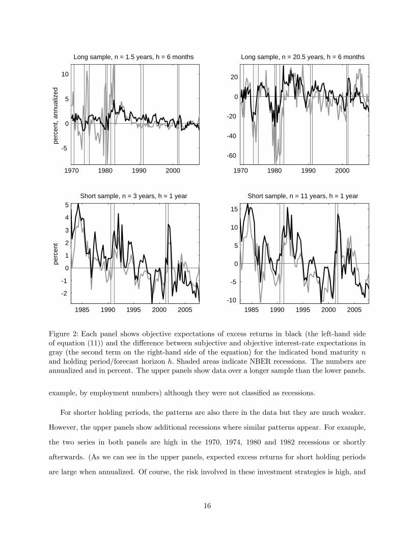
Panel B of Table 3 reports mean absolute distances between the survey forecasts and model-

implied forecasts, for both the subjective belief and the objective statistical model. Comparison of

these errors provides a measure of how well the change of measure works to capture the deviation

of survey forecasts from statistical forecasts.

1984 1986 1988 1990 1992 1994 1996 1998 2000 2002 2004

4

6

8

10

12

perc

ent

Survey forecasts and model implied forecasts; 10 year bond

surveyssubj. modelobj.model

1984 1986 1988 1990 1992 1994 1996 1998 2000 2002 2004

-0.5

0

0.5

1

1.5

perc

ent

One year forecast less objective one year forecast; 10 year bond

surveyssubj. model

Figure 3: The top panel shows one-year ahead forecasts of the 10-year zero coupon rate constructedfrom survey data in Section III, together with the corresponding forecasts from our objective andsubjective models. The bottom panel shows the difference between the survey forecast and theobjective model forecast, as well as the difference between the subjective and objective modelforecasts.

The results show that the improvement is small for short-horizon forecasts of short yields.

However, there is a marked reduction of errors for 1-year forecasts, especially for the 10-year bond.

Figure 3 shows where the improvements in matching the long-bond forecasts come from. The top

26

panel shows one-year ahead forecasts of the 10-year zero coupon rate constructed from survey data

in Section III, together with the corresponding forecasts from our objective and subjective models,

for the sample 1982:4-2007:3. All forecasts track the actual 10-year rate over this period, which

is natural given the persistence of interest rates. The largest discrepancies between the survey

forecasts and the subjective model on the one hand, and the objective model on the other hand,

occur during and after the recessions of 1990 and 2001. In both periods, the objective model quickly

forecasts a drop in the interest rate, whereas investors did not actually expect such a drop. The

subjective model captures this property.

For our asset pricing application, we are particularly interested in how well the subjective model

captures deviations of survey forecasts of long interest rates from their statistical forecasts over the

business cycle. As discussed in Section III, this forecast difference is closely related to measured

expected excess returns. The bottom panel of the figure focuses again on forecasting a 10-year rate

over one year, and plots the difference between the survey forecast and the objective model forecast,

as well as the difference between the subjective and objective model forecasts. It is apparent that

both forecast differences move closely together at business cycle frequencies, increasing during and

after recessions. We thus conclude that the subjective model is useful to capture this key fact about

subjective forecasts that matters for asset pricing.

C. Subjective risk premia

We now compare our estimated subjective risk premia to common statistical measures of objective

risk premia. The motivation is that measures of objective premia provide stylized facts that rational

expectations asset pricing models try to match. In particular, empirical evidence of predictability

of excess returns from standard predictability regressions has led to a search for sources of time

varying risk or risk aversion. The preliminary results of section III suggest that less time variation

in risk premia is required once investors’ forecast errors are taken into account. Here we quantify

how much time variation in expected excess returns is left once we move to subjective beliefs.

We focus on 1-year holding period returns on bonds with 2 and 10 years maturity. We compare

our subjective premia to three statistical measures of objective premia. The first is the fitted value

27

of a regression of excess returns on a single yield spread, the 5-year-1-quarter spread, denoted the

YS measure. In other words, we regress the excess return x(n,4)t+4 on i(20)t − i(1)t and a constant. This

regression is closely related to that in the classic Fama-Bliss study of bond return predictability,

which uses the forward-spot spread. The second measure (labelled CP measure) is the fitted

value from a regression on five yields with maturities 1,2,3, 4 and 5 years. This follows Cochrane

and Piazzesi (2005) who showed that this approach leads to substantially higher R2s. The third

measure is, for each subjective model specification, the forecast from the corresponding objective

model which provides the conditional expectation of the excess return under P .

Table 4 summarizes the properties of the regression based measures of objective premia. Ac-

cording to these measures, the volatility of the predictable part of 1-year holding period returns

is around 1% per year for the 2-year bond, and around 6% for the 10-year bond. The regression

based on five yields naturally delivers a higher R2, over 30% on both bonds. We are also interested

in the frequency properties of premia. We use a band pass filter to decompose premia into three

orthogonal components, a low frequency “trend” component (period > 8 years), a “cycle” com-

ponent (period between 1.5 and 8 years), as well as high frequency noise. The columns labelled

“trend” and “cycle” show the percentage of variance contributed by the respective components.

Since the yield spread is a key business cycle indicator, the YS measure is particularly cyclical. The

CP measure improves in part by including a larger trend component.

Table 4: Objective Premia from Regressions

maturity 2 years maturity 10 yearsRegression on yield spread (YS measure)

volatility % trend % cycle R2 volatility % trend % cycle R2

0.72 12 57 .14 6.10 12 57 .28Regression on five yields (CP measure)

volatility % trend % cycle R2 volatility % trend % cycle R2

1.08 29 40 0.31 6.29 24 50 0.30

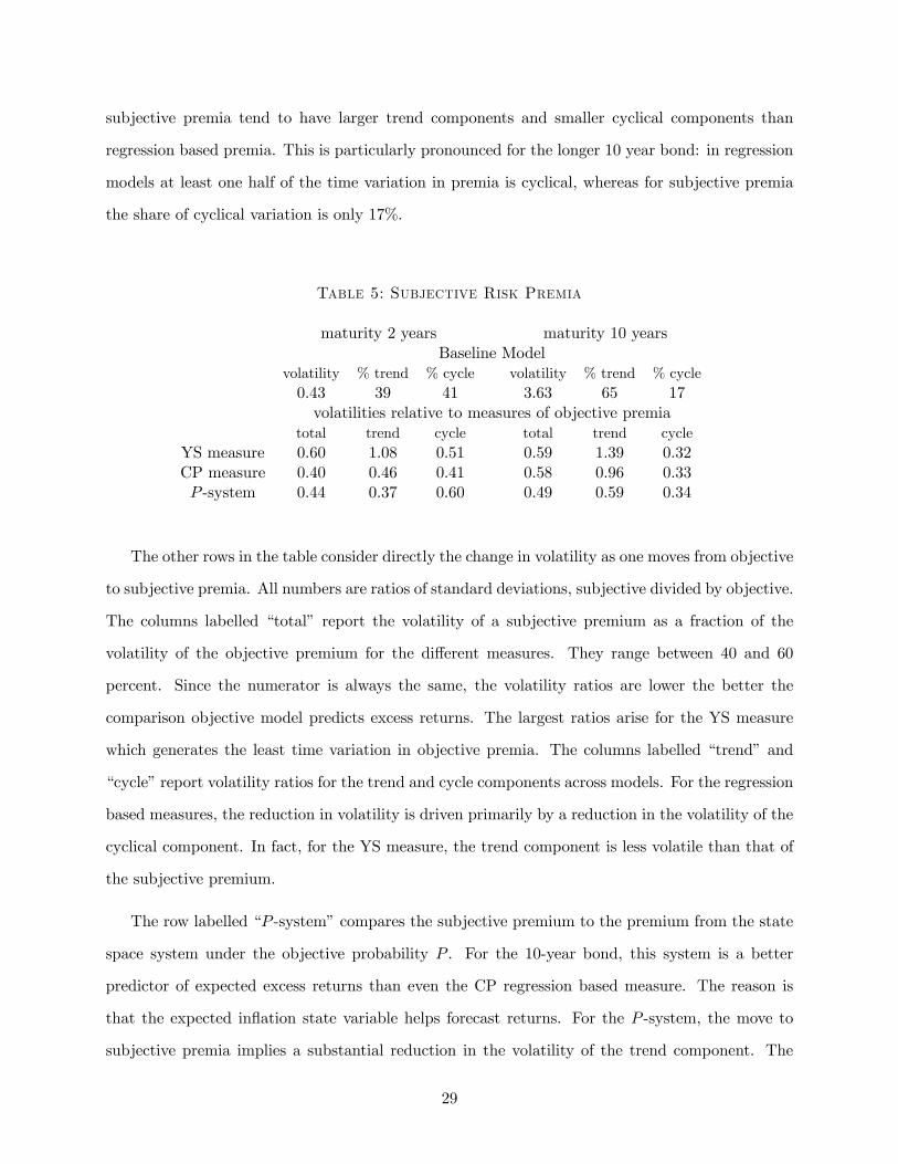
Table 5 presents a set of comparison statistics. The first line shows the properties of the

subjective premium itself. For the baseline model, the standard deviation of the one-year premium

on a 2-year bond is 43 basis points; it is 3.6% on the 10-year bond. These volatilities are substantially

smaller than those of regression measures of premia. The frequency properties are also different:

28

subjective premia tend to have larger trend components and smaller cyclical components than

regression based premia. This is particularly pronounced for the longer 10 year bond: in regression

models at least one half of the time variation in premia is cyclical, whereas for subjective premia

the share of cyclical variation is only 17%.

Table 5: Subjective Risk Premia

maturity 2 years maturity 10 yearsBaseline Model

volatility % trend % cycle volatility % trend % cycle0.43 39 41 3.63 65 17volatilities relative to measures of objective premia

total trend cycle total trend cycleYS measure 0.60 1.08 0.51 0.59 1.39 0.32CP measure 0.40 0.46 0.41 0.58 0.96 0.33P -system 0.44 0.37 0.60 0.49 0.59 0.34

The other rows in the table consider directly the change in volatility as one moves from objective

to subjective premia. All numbers are ratios of standard deviations, subjective divided by objective.

The columns labelled “total” report the volatility of a subjective premium as a fraction of the

volatility of the objective premium for the different measures. They range between 40 and 60

percent. Since the numerator is always the same, the volatility ratios are lower the better the

comparison objective model predicts excess returns. The largest ratios arise for the YS measure

which generates the least time variation in objective premia. The columns labelled “trend” and

“cycle” report volatility ratios for the trend and cycle components across models. For the regression

based measures, the reduction in volatility is driven primarily by a reduction in the volatility of the

cyclical component. In fact, for the YS measure, the trend component is less volatile than that of

the subjective premium.

The row labelled “P -system” compares the subjective premium to the premium from the state

space system under the objective probability P . For the 10-year bond, this system is a better

predictor of expected excess returns than even the CP regression based measure. The reason is

that the expected inflation state variable helps forecast returns. For the P -system, the move to

subjective premia implies a substantial reduction in the volatility of the trend component. The

29

P -system measure differs from the regression based measures in that it generates premia with larger

trend components; the shares of the trend components is 55% for the 2 year bond and 58% for the

10 year bond. These components are due to the presence of expected inflation in the system.

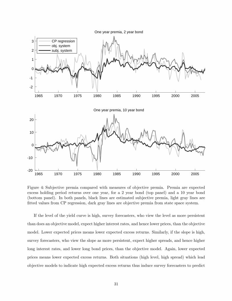
Figure 4 plots subjective premia on the two bonds together with the respective CP measures

as well as the objective premia from the state space system under P . The properties from the

table are also visible to the naked eye. Consider first the long, (10 year) bond in the bottom panel.

Both measures of objective premia show substantial cyclical movements: most recessions during

the sample period can be identified as upward spikes in objective premia, for example in 1970, 1991

and 2001. The CP measure also spikes in 1974 and 1979. Here the P -system measure responds less

to the business cycle; this is because it is driven more by expected inflation which lowers premia

during this period. In contrast to both measures of objective premia, the subjective premium on

the long bond responds only weakly to recessions. The bulk of the movement in the subjective

premium is at low frequencies: it was high in the late 1970s and early 1980s when the level of the

yield curve was high, and low towards the beginning and end of our sample.

Consider next the medium (2 year) bond. It is clear again that the subjective premium is less

volatile than the measures of objective premia. At the same time, recession periods now register as

upward spikes in all of the displayed lines. The main difference between objective and subjective

premia for the medium bond is in the trend: the subjective premium is much smaller in the late

1970s and early 1980s then the objective premia. Comparing the objective premia across maturities

(across panels), it is also apparent that objective premia on the long bond are more cyclical and

exhibit less trend than objective premia on the medium bond. For subjective premia, the situation

is the reverse.

The intuition for these results comes from the differences between survey forecasts and objective

forecasts. Under a statistical model, both the slope and the level are indicators of high expected

excess returns. For example, Figure 4 shows that measures of objective premia comove positively

with both slope and level. We have seen in the previous section that survey forecasters treat both

the level and the slope of the yield curve as more persistent than what they are under an objective

model. This difference between survey forecasts and objective forecasts of future bond prices then

weakens the effect of both indicators.

30

1965 1970 1975 1980 1985 1990 1995 2000 2005

-2

-1

0

1

2

3

One year premia, 2 year bond

CP regressionobj. systemsubj. system

1965 1970 1975 1980 1985 1990 1995 2000 2005-20

-10

0

10

20

One year premia, 10 year bond

Figure 4: Subjective premia compared with measures of objective premia. Premia are expectedexcess holding period returns over one year, for a 2 year bond (top panel) and a 10 year bond(bottom panel). In both panels, black lines are estimated subjective premia, light gray lines arefitted values from CP regression, dark gray lines are objective premia from state space system.

If the level of the yield curve is high, survey forecasters, who view the level as more persistent

than does an objective model, expect higher interest rates, and hence lower prices, than the objective

model. Lower expected prices means lower expected excess returns. Similarly, if the slope is high,

survey forecasters, who view the slope as more persistent, expect higher spreads, and hence higher

long interest rates, and lower long bond prices, than the objective model. Again, lower expected

prices means lower expected excess returns. Both situations (high level, high spread) which lead

objective models to indicate high expected excess returns thus induce survey forecasters to predict

31

lower prices and returns than the objective models. This generates the overall reduction in volatility.

The higher persistence of level and slope perceived by survey forecasters also helps explain the

different frequency properties of premia on medium (for example 2 year) and long (for example 10

year) bonds. The level of the yield curve is always relatively more important for short bonds rather

than for long bonds. This is true not only for yields themselves, but also for measures of objective

premia: those measures are driven relatively more by the slope for long bonds and relatively more

by the level for medium bonds. A move to subjective premia weakens the effect of both indicators

of high premia, the slope and the level. For a given maturity, it tends to weaken more the effect

of the indicator that is more important. The move thus makes the premium on long bonds less

responsive to the slope and it makes the premium on medium bonds less responsive to the level.

This is the effect displayed in the figure.

V Bond positions

In this section, we use the (subjective) term structure model estimated in the previous section

to represent the universe of bonds available to investors in terms of a small number of “spanning

bonds”. In subsection A., we construct, for every zero-coupon bond, a portfolio of three bonds

— a short bond and two long bonds — that replicates closely the return on the given zero-coupon

bond. In subsection B., we then show how statistics on bond positions in the US economy can be

converted into a time series of positions in the three bonds.

A. Replicating Zero Coupon Bonds

According to the term structure model, the price P(n)t of a zero coupon bond of maturity n at

date t is well described by exp (An +B0nft). We now select N long bonds, zero-coupon bonds with

maturity greater than one, and stack their coefficients in a vector ba and a matrix bb. Our goal isto construct a portfolio containing the long bonds and the short bond such that the return on the

portfolio replicates closely the return on any other zero-coupon bond with maturity n. We use a

discretization of continuous time returns, similar to those used above for the return on wealth. We

32

approximate the change in price on an n-period bond by

P(n−1)t+1 − P

(n)t ≈ P

(n)t

µAn−1 −An +B0n−1(ft+1 − ft) + (Bn−1 −Bn)

0ft +1

2B0n−1σfσ

0fB

0n−1

¶= P

(n)t

µAn−1 −An +B0n−1μ

∗f +B0n−1(φ

∗f − I)ft + (Bn−1 −Bn)

0ft +1

2B0n−1σfσ

0fB

0n−1

¶+P

(n)t B0n−1σfε

∗t+1

= : a(n)t + b

(n)t σfε

∗t+1(16)

Conditional on date t, we thus view the change in value of the bond as an affine function in

the shocks to the factors σfε∗t+1. Its distribution is described by N +1 time-dependent coefficients:

the constant a(n)t and the loadings b(n)t on the N shocks. In particular, we can calculate coefficients³a(1)t , b

(1)t

´for the short bond, and we can arrange coefficients for the N long bonds in a vector at

and a matrix bt. Now consider a portfolio that contains θ1 units of the short bond and θi units

of the ith long bond. The change in value of this portfolio is also an affine function in the factor

shocks and we can set it equal to the change in value of any n-period bond:

(17)³θ1 θ

0´⎛⎜⎝ a(1)t b

(1)t

at bt

⎞⎟⎠⎛⎜⎝ 1

σfε∗t+1

⎞⎟⎠ =

µa(n)t b

(n)t

¶⎛⎜⎝ 1

σfε∗t+1

⎞⎟⎠ .

Since the (N + 1)×(N + 1) matrix of coefficient on the left hand side is invertible for a nondegener-

ate term structure model, we can select the portfolio³θ1 θ

0´to make the conditional distribution

of the value change in the portfolio equal to that of the bond.

Replicating portfolios based on a two-factor model

When stated in terms of units of bonds³θ1, θ

´, the replicating portfolio for the n-period bond

answers the question: how many spanning bonds are equivalent to one n-period bond? For our work

below it is more convenient to define portfolio weights that answer the question: how many dollars

worth of spanning bonds are equivalent to one dollar worth of invested in the n-period bonds? The

answer to this question can be computed using the units³θ1, θ

´and the prices of spanning bonds.

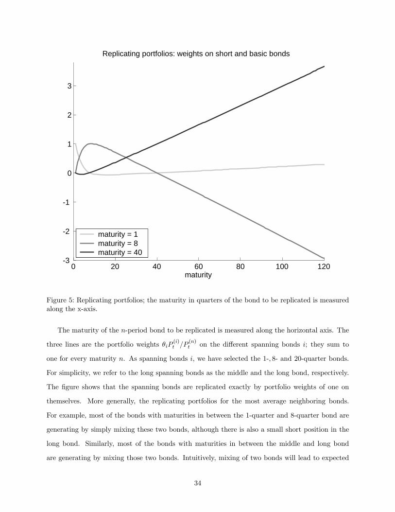
Figure 5 provides the answer computed from the two-factor term structure model estimated above.

Since the term structure model is stationary, these weights do not depend on calendar time.

33

0 20 40 60 80 100 120-3

-2

-1

0

1

2

3

Replicating portfolios: weights on short and basic bonds

maturity

maturity = 1maturity = 8maturity = 40

Figure 5: Replicating portfolios; the maturity in quarters of the bond to be replicated is measuredalong the x-axis.

The maturity of the n-period bond to be replicated is measured along the horizontal axis. The

three lines are the portfolio weights θiP(i)t /P

(n)t on the different spanning bonds i; they sum to

one for every maturity n. As spanning bonds i, we have selected the 1-, 8- and 20-quarter bonds.

For simplicity, we refer to the long spanning bonds as the middle and the long bond, respectively.

The figure shows that the spanning bonds are replicated exactly by portfolio weights of one on

themselves. More generally, the replicating portfolios for the most average neighboring bonds.

For example, most of the bonds with maturities in between the 1-quarter and 8-quarter bond are

generating by simply mixing these two bonds, although there is also a small short position in the

long bond. Similarly, most of the bonds with maturities in between the middle and long bond

are generating by mixing those two bonds. Intuitively, mixing of two bonds will lead to expected

34

returns that are linear in maturity, whereas adding a third bond helps generate curvature.

Quality of the approximation

We now provide some evidence that the approximation of a zero-coupon bond by a portfolio of

spanning bonds is decent for our purposes. There are two dimensions along which we would like to

obtain a good approximation. First, we would like the value of the approximating portfolio to be

the same as the value of the zero-coupon bond. This is relevant for measuring the supply of bonds:

below we will take existing measures of the quantity of zero-coupon-bonds held by households and

convert them into portfolios of the small number of spanning bonds that are tradable by agents in

our model. Along this dimension, the approximation is essentially as good as the term structure

model itself. For a replicating portfolio defined by (17), the portfolio value e−itθ1 + P 0t θ differs

from the bond value P (n)t only to the extent that the term structure model does not fit bonds of

maturity n. The additional approximation error introduced by the matching procedure is less than

.0001 basis points.

Second, we would like the conditional distribution of bond returns to be the same as that of

the portfolio return. This is important because we would like agents in our model to have bond

investment opportunity sets that are similar to those of actual households who trade bonds of many

more maturities. Figure 6 gives an idea about the goodness of the approximation (17) by comparing

statistics of the actual return implied by the term structure model and the approximating return.

All statistics are unconditional moments computed from our sample, using the realizations of the

term structure factors. For example, to obtain the difference in means in the top panel, we compute

(i) quarterly returns from the term structure model using the formula exp (An +B0nft) for prices,

and (ii) quarterly returns based on the approximate formula for price changes (16) and subtract

the mean of (i) from the mean of (ii).

On average, the two return distributions are quite similar for all maturities. The mean returns

differ by less than 10 basis points for all bonds shorter than 30 years. The difference in variance is

at most 30 basis points. The approximation error increases with maturity, as do the mean return

and the variance of returns themselves. The approximate mean return on bonds is always within

5% of the true mean return, while the approximate variance is within 5-15% of the true variance.

35

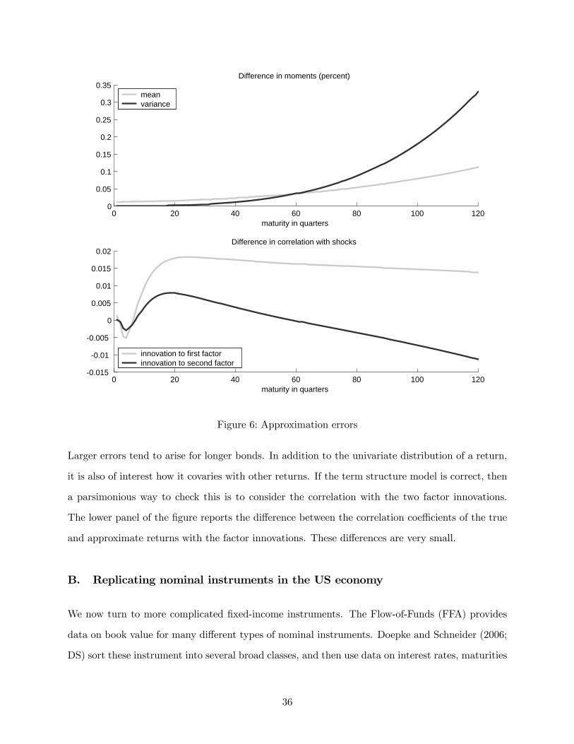
0 20 40 60 80 100 120-0.015

-0.01

-0.005

0

0.005

0.01

0.015

0.02Difference in correlation with shocks

maturity in quarters

innovation to first factorinnovation to second factor

0 20 40 60 80 100 1200

0.05

0.1

0.15

0.2

0.25

0.3

0.35Difference in moments (percent)

maturity in quarters

meanvariance

Figure 6: Approximation errors

Larger errors tend to arise for longer bonds. In addition to the univariate distribution of a return,

it is also of interest how it covaries with other returns. If the term structure model is correct, then

a parsimonious way to check this is to consider the correlation with the two factor innovations.

The lower panel of the figure reports the difference between the correlation coefficients of the true

and approximate returns with the factor innovations. These differences are very small.

B. Replicating nominal instruments in the US economy

We now turn to more complicated fixed-income instruments. The Flow-of-Funds (FFA) provides

data on book value for many different types of nominal instruments. Doepke and Schneider (2006;

DS) sort these instrument into several broad classes, and then use data on interest rates, maturities

36

and contract structure to construct, for every asset class and every date t, a certain net payment

stream that the holders of the asset expect to receive in the future. Their procedure takes into

account credit risk in instruments such as corporate bonds and mortgages. They use these payment

streams to restate FFA positions at market value and assess the effect of changes in inflation

expectations on wealth.

Here we determine, for every broad asset class, a replicating portfolio that consists of spanning

bonds. For every asset class and every date t, DS provide a certain payment stream, which we can

view as a portfolio of zero-coupon bonds. By applying equation (17) to every zero-coupon bond,

and then summing up the resulting replicating portfolios across maturities, we obtain a replicating

portfolio for the asset class at date t. Figure 7 illustrates replicating portfolios for Treasury bonds

and mortgages. The top panel shows how the weights on the spanning bonds in the replicating

portfolio for Treasury bonds have changed over the postwar period.

The reduction of government debt after the war went along with a shortening of maturities:

the weight on the longest bond declined from over 60% in 1952 to less than 20% in 1980. This

development has been somewhat reversed since 1980.6 The bottom panel shows that the effective

maturity composition of mortgages was very stable before the 1980s, with a high weight on long

bonds. The changes that apparent since the 1980s are driven by the increased use of adjustable

rate mortgages.

We do not show replicating portfolios for Treasury bills, municipal bonds and corporate bonds,

since the portfolio weights exhibit few interesting changes over time. All three instruments are

represented by essentially constant portfolios of only two bonds: T-bills correspond to about 80%

short bonds and 20% middle bonds, that for corporate bonds corresponds to about 60% middle

bonds and 40% long bonds, and the replicating portfolio for municipal bonds has 70% long bonds

and 30% middle bonds. The final asset class is a mopup group of short instruments, which we

replicate by a short bond.

Replicating aggregate FFA household sector positions

We compute measure aggregate household holdings in the FFA at date t. To derive their

6The figure shows only the portfolios corresponding to outstanding Treasury bonds, not including bills. DS usedata from the CRSP Treasury data base to construct a separate series for bills.

37

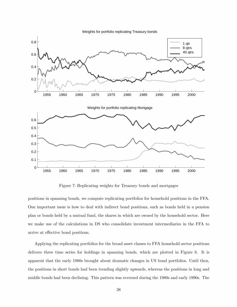
1955 1960 1965 1970 1975 1980 1985 1990 1995 20000

0.2

0.4

0.6

0.8

Weights for portfolio replicating Treasury bonds

1 qtr 8 qtrs 40 qtrs

1955 1960 1965 1970 1975 1980 1985 1990 1995 20000

0.1

0.2

0.3

0.4

0.5

0.6

Weights for portfolio replicating Mortgage

Figure 7: Replicating weights for Treasury bonds and mortgages

positions in spanning bonds, we compute replicating portfolios for household positions in the FFA.

One important issue is how to deal with indirect bond positions, such as bonds held in a pension

plan or bonds held by a mutual fund, the shares in which are owned by the household sector. Here

we make use of the calculations in DS who consolidate investment intermediaries in the FFA to

arrive at effective bond positions.

Applying the replicating portfolios for the broad asset classes to FFA household sector positions

delivers three time series for holdings in spanning bonds, which are plotted in Figure 8. It is

apparent that the early 1980s brought about dramatic changes in US bond portfolios. Until then,

the positions in short bonds had been trending slightly upwards, whereas the positions in long and

middle bonds had been declining. This pattern was reversed during the 1980s and early 1990s. The

38

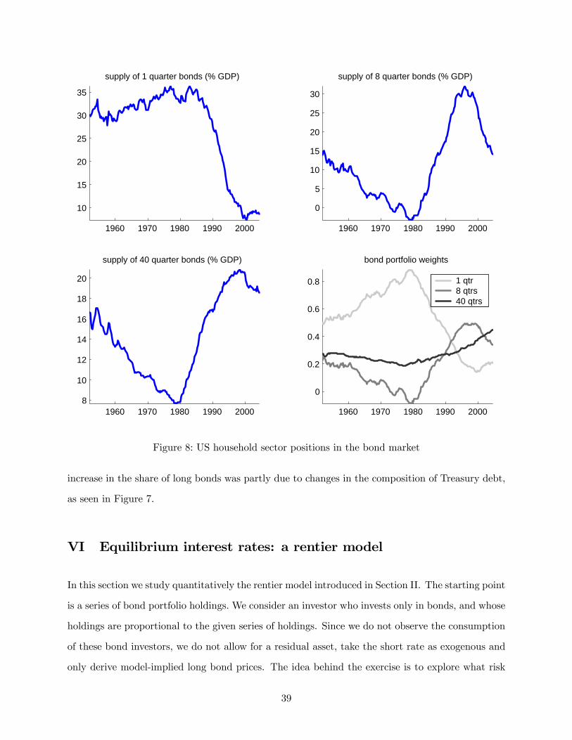
1960 1970 1980 1990 2000

10

15

20

25

30

35

supply of 1 quarter bonds (% GDP)

1960 1970 1980 1990 2000

0

5

10

15

20

25

30

supply of 8 quarter bonds (% GDP)

1960 1970 1980 1990 20008

10

12

14

16

18

20

supply of 40 quarter bonds (% GDP)

1960 1970 1980 1990 2000

0

0.2

0.4

0.6

0.8

bond portfolio weights

1 qtr8 qtrs40 qtrs

Figure 8: US household sector positions in the bond market

increase in the share of long bonds was partly due to changes in the composition of Treasury debt,

as seen in Figure 7.

VI Equilibrium interest rates: a rentier model

In this section we study quantitatively the rentier model introduced in Section II. The starting point

is a series of bond portfolio holdings. We consider an investor who invests only in bonds, and whose

holdings are proportional to the given series of holdings. Since we do not observe the consumption

of these bond investors, we do not allow for a residual asset, take the short rate as exogenous and

only derive model-implied long bond prices. The idea behind the exercise is to explore what risk

39

premia look like if there is a subset of investors for whom bonds are very important.

Formally, the input to the rentier exercise is a sequence of portfolio weights bωt = Bt/Bt that

represents the class of bonds considered in terms of our spanning bonds, a sequence of observed

short-term interest rates, as well as a sequence of subjective beliefs P ∗t about future interest rates

and inflation that is needed to solve the portfolio choice problem. The latter sequence of beliefs

consists of a sequence of conditionals from the subjective probability distribution over yields and

inflation estimated in subsection B.. The exercise proceeds by deriving portfolio demand and solving

out for equilibrium prices from equation (9).

Portfolio choice with subjective return distributions driven by a normal VAR

When subjective beliefs are represented by a linear system with normal shocks, tractable ap-

proximate formulas for investors’ portfolio policies and equilibrium prices are available. Subjective

beliefs about term structure factors and inflation are represented by (4). The log short interest

rate it+1 and log inflation πt+1 are linear functions of ht+1 and log excess returns xt+1 are linear

functions of st+1 and st. The real return on the short bond it+1 − πt+1 and the excess returns on

the other bonds xt+1 can thus also be represented as a state space system with state vector st. The

state vector for the household problem is therefore¡W t, st

¢.

We use the approximation method proposed by Campbell, Chan and Viceira (2003). The basic

idea is that the log return on a portfolio in a discrete time problem is well approximated by a

discretized version of its continuous-time counterpart. In our setup, the log return on wealth is

approximated by

(18) logRwt+1 ≈ it − πt+1 + ω>t xt+1 +

1

2ω>t (diag (Σxx)−Σxxωt) ,

where Σxx is the one-step-ahead conditional covariance matrix of excess returns xt+1, and ωt is the

vector of portfolio weights on the long bonds.

If this approximation is used for the return on wealth, the investor’s value function can be written

as vt¡W t, st

¢= logW t + v(st+1), where v is linear-quadratic in the state vector st. Moreover, the

40

optimal portfolio is

ωt ≈1

γΣ−1xx

µE∗t [xt+1] +

1

2diag (Σxx)

¶+

µ1− 1

γ

¶Σ−1xx cov

∗t (xt+1, πt+1)(19)

−µ1− 1

γ

¶Σ−1xx cov

∗t (xt+1, v(st+1)) .

If γ = 1 — the case of separable logarithmic utility — the household behaves “myopically”, that is, the

portfolio composition depends only on the one-step-ahead subjective distribution of returns. More

generally, the first line in (19) represents the myopic demand of an investor with one-period horizon

and risk aversion coefficient γ. To obtain intuition, consider the case of independent returns, so

that Σxx is diagonal. The first term then says that the myopic investor puts more weight on assets

with high expected returns and low variance, and more so when risk aversion is lower. The second

term says that, if γ > 1, the investor also likes assets that provide insurance against inflation, and

buys more such insurance assets if risk aversion is higher. For general Σxx, these statements must

be modified to take into account correlation patterns among the individual assets.

For a long-lived household with γ 6= 1, asset demand also depends on the covariance of excessreturns and future continuation utility v (st+1). Continuation utility is driven by changes in in-

vestment opportunities: a realization of st+1 that increases v is one that signals high returns on

wealth (“good investment opportunities”) in the future. Agents with γ > 1 prefer relatively more

asset payoff in states of the world where investment opportunities are bad. As a result, an asset

that pays off when investment opportunities are bad is attractive for a high-γ agent. He will thus

demand more of it than a myopic agent.

Explicit price formulas

Substituting the portfolio policy (19) into (9), we can explicitly solve out for long bond prices. To

clarify the effect of subjective expectations, we also add and subtract the objective price expectation

Etpt+1 to arrive at

pt = −it +Etpt+1 +1

2diag (Σxx)

+E∗t pt+1 −Etpt+1

−γΣxxbωt + (γ − 1) cov∗t (xt+1, πt+1)− (γ − 1) cov∗t (xt+1, v(st+1)) .(20)

41

According to the first line of this formula, the price of the long bond is determined as the (log)

discounted expected future price (where the variance term appears because of Jensen’s inequality).

For a moment, suppose that the expressions in the other lines are constant. In this case, the prices

are determined according to the expectations hypothesis: on average (up to a constant), buying a

long bond at t and holding it to maturity should cost the same as buying a short bond at t, earning

interest it on it and then buying the long bond only at t+ 1.

The remaining lines of this formula may lead to deviations from the expectations hypothesis,

and thus to time-varying expected excess returns. The two lines give two seperate seasons for

such deviations. The second line in the formula says that we may observe deviations from the

expectations hypothesis because investors may have expectations that are not rational. In this

case, investors’ subjective expectation of bond payoffs E∗t bpt+1 differs from the objective expectationEtbpt+1. The third line in the formula represents subjective risk premia, which may also changeover time. In particular, they may change as the composition of investor portfolios ωt changes over

time. Below, we discuss these mechanism in detail.

Suppose that investors have expectations of future prices that are not rational so that subjective

expectations E∗t bpt+1 differ from objective expectations Etbpt+1. This implies that even if subjectiverisk premia (in the third line of the formula) are constant, the modeler may be able to predict

excess returns on long bonds with some variable known at time t. This predictability reflects the

systematic forecast errors E∗t pt+1 −Etpt+1 made by investors.

But even if expectations are rational, there are subjective risk premia which may change over

time. These premia compensate investors for holding a risky long bond for three reasons. First,

investors with Epstein-Zin utility demand compensation for holding assets whose returns covary

with the return on wealth. This is captured by the conditional covariance Σxxbωt, which is thecovariance of excess returns on bonds with the excess return on wealth, bω>t bxt+1 from equation

(18). Since the composition of wealth bωt changes over time, with changes in the relative amountof different bonds in Bt, so there can be time variation in risk premia. In the case of log utility

(γ = 1) this covariance represents the entire risk premium. More generally, a higher risk aversion

coefficient drives up the compensation required for covariance with the return on wealth.7

7Since consumption is proportional to savings, or wealth, the first term in the risk premium also represents the

42

Second, there is a premium for covariance with future investment opportunities. An asset

that insures households against bad future investment opportunities — by paying off less when

continuation utility vt+1 is high — commands a lower premium. Hedging against future opportunities

also changes the inflation risk premium. For γ > 1, households have to be compensated less to hold

an asset that provides insurance against inflation.

A. Numerical results

The inputs are a sequence of portfolio weights and a system for returns. For the weights, we

have used US households’ holdings of Treasury bonds, their holdings of all nominal assets except

deposits, as well as US households’ net position of nominal assets. The main lessons have been

similar for all cases. In what follows, we report only the results for the total net position.

Table 6: Subjective Moments of Excess Returns (% p.a.)

excess returns (%) 2 year 10 year

mean 0.80 1.16

cond. standard deviation 2.78 13.72

cond. correlation matrix 1 0.811

correlation with short bond 0.19 0.08

Under the subjective system from Section IV, the short bond has a subjective mean real return

of 1.80% and a one-quarter-ahead conditional volatility of 0.58%, both in annualized percentage

terms. Table 6 summarizes other relevant moments of the subjective distribution of quarterly

excess returns implied by the model for the middle and long spanning bonds (maturities of 2

and 10 years, respectively) In terms of conditional Sharpe ratios (mean excess return divided by

standard deviation), the middle bonds looks more attractive than the long bond. It is also notable

that the long and middle bond returns are highly positively correlated. No longer bond covaries

much with the short bond return. We have also seen that the subjective belief generates a role for

covariance of returns with consumption growth, multiplied by risk aversion.

43

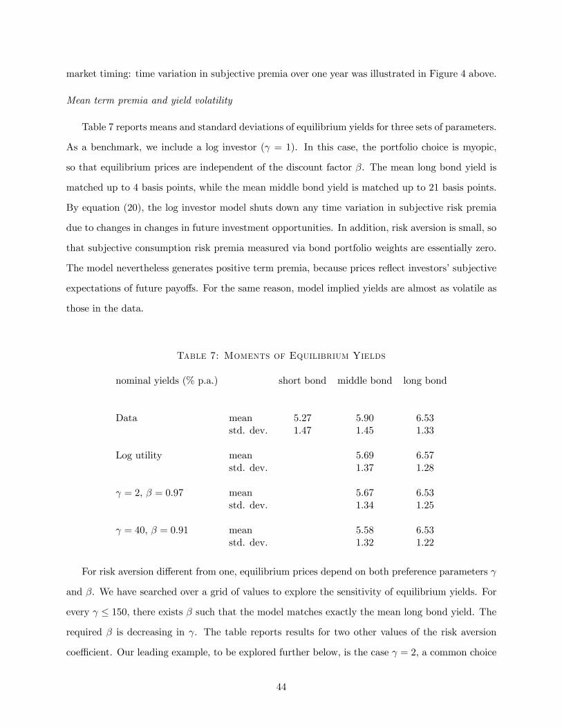
market timing: time variation in subjective premia over one year was illustrated in Figure 4 above.

Mean term premia and yield volatility

Table 7 reports means and standard deviations of equilibrium yields for three sets of parameters.

As a benchmark, we include a log investor (γ = 1). In this case, the portfolio choice is myopic,

so that equilibrium prices are independent of the discount factor β. The mean long bond yield is

matched up to 4 basis points, while the mean middle bond yield is matched up to 21 basis points.

By equation (20), the log investor model shuts down any time variation in subjective risk premia

due to changes in changes in future investment opportunities. In addition, risk aversion is small, so

that subjective consumption risk premia measured via bond portfolio weights are essentially zero.

The model nevertheless generates positive term premia, because prices reflect investors’ subjective

expectations of future payoffs. For the same reason, model implied yields are almost as volatile as

those in the data.

Table 7: Moments of Equilibrium Yields

nominal yields (% p.a.) short bond middle bond long bond

Data mean 5.27 5.90 6.53std. dev. 1.47 1.45 1.33

Log utility mean 5.69 6.57std. dev. 1.37 1.28

γ = 2, β = 0.97 mean 5.67 6.53std. dev. 1.34 1.25

γ = 40, β = 0.91 mean 5.58 6.53std. dev. 1.32 1.22

For risk aversion different from one, equilibrium prices depend on both preference parameters γ

and β. We have searched over a grid of values to explore the sensitivity of equilibrium yields. For

every γ ≤ 150, there exists β such that the model matches exactly the mean long bond yield. Therequired β is decreasing in γ. The table reports results for two other values of the risk aversion

coefficient. Our leading example, to be explored further below, is the case γ = 2, a common choice

44

for risk aversion in macro models; matching the long rate then requires β = 0.97. The resulting

summary statistics are quite close to the log investor case. Relative to the log case, the mean long

rate falls, even though risk aversion has gone up. This is because a patient investor can hold the

long bond to hedge against bad investment opportunities, that is, low future short interest rates.

This reduces the required compensation for risk.

The table also provides a high risk aversion example: for γ = 40, we must pick β = 0.91 to

match the mean long rate. As risk aversion increases, the desire to hedge becomes stronger which

by itself would increase the demand for the long bond and lower the long rate. The reduction in β

weakens the hedging motive to keep the mean long rate at its observed value. This tradeoff says

that if high risk aversion of rentiers is to be consistent with yield spreads in the data, then the

effective planning horizon of the rentier must be shorter than that of the typical RBC agent.

There does not exist β and γ in order to find values that match exactly the mean excess returns

on both the 2 year and the 10 year yields. This is somewhat surprising, since the parameters β

and γ do have different effects on portfolio demand. In particular, higher risk aversion γ lowers

the myopic demand for bonds, but increases the hedging demand for assets that provide insurance

against bad future investment opportunities. In contrast, the discount factor affects only the size

of the hedging demand: provided that γ 6= 1, increasing β makes hedging demand more importantrelative to myopic demand. However, it appears that the myopic and hedging demands for the

two bonds react to both parameters in a similar way, so that they cannot be identified from the

two average premia. In fact, the mean spread between the long and middle bond reacts very

little to changes in β and γ. The reason is that it is due in part to systematic differences in

payoff expectations between the two bonds (induced by the subjective model), which affect prices

independently of the risk premium terms that are responsive to γ and β.

Model-implied yield spreads

Figure 9 plots yield spreads from the data together with yield spreads implied by the model

for the case γ = 2, β = 0.97. The middle panel shows that the model matches the 10-year spread

quite well. The top and bottom panel show the two-year spread, as well as the spread of the ten

year rate over the two year rate, respectively. Both panels reflects the fact that the mean 2-year

45

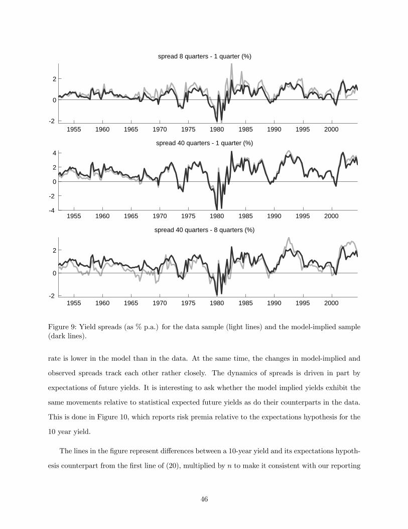
1955 1960 1965 1970 1975 1980 1985 1990 1995 2000-2

0

2

spread 8 quarters - 1 quarter (%)

1955 1960 1965 1970 1975 1980 1985 1990 1995 2000-4

-2

0

2

4spread 40 quarters - 1 quarter (%)

1955 1960 1965 1970 1975 1980 1985 1990 1995 2000-2

0

2

spread 40 quarters - 8 quarters (%)

Figure 9: Yield spreads (as % p.a.) for the data sample (light lines) and the model-implied sample(dark lines).

rate is lower in the model than in the data. At the same time, the changes in model-implied and

observed spreads track each other rather closely. The dynamics of spreads is driven in part by

expectations of future yields. It is interesting to ask whether the model implied yields exhibit the

same movements relative to statistical expected future yields as do their counterparts in the data.

This is done in Figure 10, which reports risk premia relative to the expectations hypothesis for the

10 year yield.

The lines in the figure represent differences between a 10-year yield and its expectations hypoth-

esis counterpart from the first line of (20), multiplied by n to make it consistent with our reporting

46

of premia in previous sections:

n

µi(n)t −

h

ni(h)t −

(n− h)

nEti

(n−h)t+h − 1

2vart

³x(n,h)t+1

´¶,

where x(n)t+1 is the 1-quarter excess holding period return on the n-period bond. In other words, the

lines show the difference between the forward rate on a contract that promises an (n − 1)-periodbond one period from date t. The three lines differ in what forward rate is used, and how the

expectation is formed. The light gray line labelled “data — obj. EH” shows the difference between

the forward rate from the data and the expected rate under the objective probability. It is thus

corresponds to measured expected excess returns, which tend to be high during and after recessions.

The black line represents a model implied objective risk premium — the difference between the

forward rates implied by the model and the expected rates under the objective probability. It

exhibits both a low frequency component and a business cycle component that comoves with the

risk premium from the data. To illustrate the source of these movements, the dark gray lines

show the subjective risk premia that is, differences between the forward rate implied by the model

and the expected rate under the subjective probability. The subjective premia are smoother and

contain more trend than the objective premia. Instead, those movements are due to the differences

between subjective and objective forecasts documented in Sections III.

Investors’ subjective perception of risk is reflected in the subjective risk premium, and is also

responsible for the low frequency components in the model implied objective risk premium. For

one quarter premia, equation (20) says that changes in the subjective premium must be due to

changes in hedging opportunities or changes in bond positions. At the current parameter values,

risk aversion is low and changes in positions do not have large effects. Instead, the V-shaped

pattern in the subjective risk premium is due to changes in the covariance between long bond

returns and future continuation utility. Intuitively, the insurance that long bonds provide to long

horizon investors against drops in future short rates became more valuable in the 1980s when short

rates were high. As a result, the compensation required for holding such bonds declined.

For longer horizon premia, the subjective expectation of the bond price at the end of the horizon

reflects properties of interest rate expectations beyond the next quarter. Interestingly, the market

47

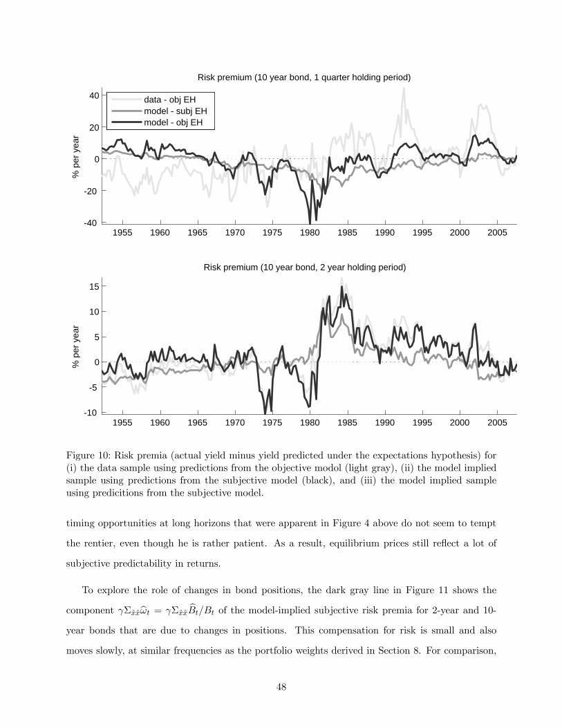
1955 1960 1965 1970 1975 1980 1985 1990 1995 2000 2005-40

-20

0

20

40

% p

er y

ear

Risk premium (10 year bond, 1 quarter holding period)

data - obj EHmodel - subj EHmodel - obj EH

1955 1960 1965 1970 1975 1980 1985 1990 1995 2000 2005-10

-5

0

5

10

15

Risk premium (10 year bond, 2 year holding period)

% p

er y

ear

Figure 10: Risk premia (actual yield minus yield predicted under the expectations hypothesis) for(i) the data sample using predictions from the objective modol (light gray), (ii) the model impliedsample using predictions from the subjective model (black), and (iii) the model implied sampleusing predicitions from the subjective model.

timing opportunities at long horizons that were apparent in Figure 4 above do not seem to tempt

the rentier, even though he is rather patient. As a result, equilibrium prices still reflect a lot of

subjective predictability in returns.

To explore the role of changes in bond positions, the dark gray line in Figure 11 shows the

component γΣxxbωt = γΣxx bBt/Bt of the model-implied subjective risk premia for 2-year and 10-

year bonds that are due to changes in positions. This compensation for risk is small and also

moves slowly, at similar frequencies as the portfolio weights derived in Section 8. For comparison,

48

the figure also shows, at different scales, low frequency components of the respective term spreads

that have been extracted using a band-pass filter. The increase in the spread in the 1980s thus

went along with a shift towards longer bond positions that contributed positively to risk premia.

However, the drop in subjective risk premia before 1980s did not go along with movements in the

spread.

The quantitative lessons of this section are confirmed when we start the exercise from other

classes of bond portfolios. Matching the long interest rate under the subjective model point us to

small risk aversion coefficients, which in turn make the contribution of subjective risk premia, and

especially the part due to bond positions, is quantitatively small. A qualitative difference is that

when we eliminate deposits and liabilities from the portfolio, the middle and long bonds become

relatively more important, and there is some evidence of business cycle variation in the model

implied subjective risk premia. This suggests that a different model of conditional variance might

lead to a larger role for subjective risk premia measured via bond positions.

49

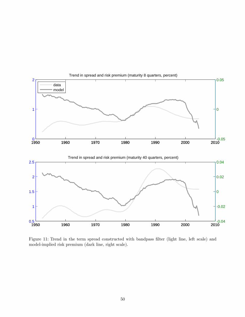
1950 1960 1970 1980 1990 2000 20100

1

2Trend in spread and risk premium (maturity 8 quarters, percent)

1950 1960 1970 1980 1990 2000 2010-0.05

0

0.05datamodel

1950 1960 1970 1980 1990 2000 20100.5

1

1.5

2

2.5Trend in spread and risk premium (maturity 40 quarters, percent)

1950 1960 1970 1980 1990 2000 2010-0.04

-0.02

0

0.02

0.04

Figure 11: Trend in the term spread constructed with bandpass filter (light line, left scale) andmodel-implied risk premium (dark line, right scale).

50

References

Ang, A., Bekaert, G., Wei, M. 2007. Do Macro Variables, Asset Markets or Surveys ForecastInflation better? Journal of Monetary Economics 54, 1163-1212.

Bacchetta, P., Mertens, E., van Wincoop, E. 2008. Predictability in Financial Markets: What doSurvey Expectations tell us? Manuscript, Lausanne.

Backus, D., Gregory, A., Zin, S. 1989. Risk Premiums in the Term Structure: Evidence fromArtificial Economies. Journal of Monetary Economics 24, 371-399.

Bansal, R., A. Yaron 2004. Risks for the long run: A potential resolution of asset pricing puzzles.Journal of Finance 59, 1481-1509.

Campbell, J.Y., Chan Y.L., Viceira, L.M. 2003. A Multivariate Model of Strategic Asset Alloca-tion. Journal of Financial Economics 67(1), 41-80.

Campbell, J.Y., Viceira, L.M. 2001. Who should buy long-term bonds? American EconomicReview 91(1), 99-127.

Chun, A.L. 2006. Expectations, Bond Yields and Monetary Policy. Manuscript, University ofMontreal.

Cochrane, J.H., M. Piazzesi 2005. Bond Risk Premia. American Economic Review 95:1, 138-160.

Cogley, T. 2005. Changing Beliefs and the Term Structure of Interest Rates: Cross-EquationRestrictions with Drifting Parameters. Review of Economic Dynamics 8, pp.

Dai, Q., K.J. Singleton 2002. Expectation Puzzles, Time-varying Risk Premia, and Affine Modelsof the Term Structure Journal of Financial Economics 63, 415-441.

Doepke, M., Schneider M. 2006. Inflation and the Redistribution of Nominal Wealth. Journal ofPolitical Economy 114(6), 1069-1097.

Epstein, L., Zin, S. 1989. Substitution, risk aversion and the temporal behavior of consumptionand asset returns: a theoretical framework. Econometrica 57, 937-69

Fama, E.F., Bliss, R.R.. The Information in Long-Maturity Forward Rates. American EconomicReview, 1987, (77), 680-92.

Frankel, J.A., Froot, K. 1987. Using Survey Data to Test Standard Propositions RegardingExchange Rate Expectations. American Economic Review 77, 133-153.

Friedman, Ben. 1980. Survey Evidence on the ‘Rationality’ of Interest-Rate Expectations. Journalof Monetary Economics 6, 453-465.

Froot, K. 1989. New Hope for the Expectations Hypothesis of the Term Structure of InterestRates. Journal of Finance, 44, pp. 283-305.

Gourinchas, P.0., Tornell A. 2005. Exchange Rate Dynamics, Learning, and Misperception. Jour-nal of International Economics 64, pp. 303-333.

Greenwood, J. and D. Vayanos 2007, Bond Supply and Expected Excess Returns. Manuscript,HBS and LSE.

51

Gürkaynak, R.S., Sack, B., Wright, J.H., 2006. The U.S. Treasury Yield Curve: 1961 to thePresent. Manuscript, Federal Reserve Board of Governors.

Hansen, L.P., J.C. Heaton, and N. Li 2005. Consumption strikes back? Measuring Long RunRisk. Manuscript, University of Chicago.

Kim, D., A. Orphanides 2007. Term Structure Estimation with Survey Data on Interest RateForecasts. Manuscript, Federal Reserve Board.

Krishnamurthy, A., Vissing-Jorgensen, A. 2007. The Demand for Treasury Debt. NBER WorkingPaper #12881.

Lucas, R.E. Jr. 1978. Asset Prices in an Exchange Economy. Econometrica 46, 1429-1445.

Piazzesi, M., Schneider, M. 2006. Equilibrium Yield Curves. NBER Macroannual 2006.

Wachter, J. 2006. A Consumption-Based Model of the Term Structure of Interest Rates. Journalof Financial Economics 79, 365-399.

52

A Appendix

Table 1 A reports maximum likelihood estimates of the objective state space system (2). The

quarterly data sample is 1964:1-2007:4.

Table 1 A: Estimation of Objective System

μ× 100 ηh chol(Ω)

short rate 1.47 0.88 0.12 0.13. 0.26— (0.04) (0.08) (0.05) (0.01)

spread 0.27 0.05 0.76 -0.06 -0.13 0.13— (0.03) (0.06) (0.03) (0.01) (0.01)

exp. inflation 0.98 0 0 1 0.04 0.03 0.27— (0.02) (0.02) (0.01)

φs σs

short rate 0.88 0.12 0.13 1(0.04) (0.08) (0.05)

spread 0.05 0.76 -0.06 0 1(0.03) (0.06) (0.03)

exp. inflation -0.04 -0.08 0.97 0.13 -0.09 0.53(0.03) (0.06) (0.04) (0.11) (0.16) (0.09)

NOTE: This table contains maximum-likelihood estimates of the state space system

ht = μ+ ηst−1 + et

st = φsst−1 + σset.

“chol(Ω)” denotes the Cholesky decomposition of var(et) = Ω. Brackets indicate maximum-likelihood asymptotic standard errors computed from the Hessian.

53

Table 2A: Estimation of Market Prices of Risk

λ0 λ1short rate spread exp. inflation

short rate -0.20 -0.13 -0.11 0.13spread 0.09 0.05 -0.08 -0.06

λ∗0 λ∗1

short rate -0.01 -0.01 -0.14 0.03spread -0.04 -0.03 0.08 -0.05

NOTE: This table contains nonlinear least-squares estimates of the first two rows ofobjective market price of risk parameters λt = l0+l1st and their subjective counterparts.

B Appendix

The goal of this appendix is to describe an equilibrium model of the US economy. The equations

about optimal behavior and model-implied prices described in the body of the paper (for the case

with a residual asset) hold in this equilibrium model. The model goes beyond these equations

because it (i) derives initial wealth of households as the (endogenous) value of exogenous quantities

of asset endowments and (ii) and specifies trades between US households and other sectors of the

economy, such as foreigners. The households in the model optimize for some given exogenous

expectations. This specification allows expectations to be consistent with survey evidence or with

some learning mechanism.

The model describes a single trading period t. In each period, the US household sector trades

assets with another sector of the economy. We call the other sector the “rest of the economy”

(ROE), which stands in for the government, business, and foreign sectors. Households enter the

trading period t endowed with one unit of the residual asset. Their initial wealthW t also comprises

dividends from the residual asset as well as the value of all bonds written on the rest of the economy

that households bought at date t− 1, denoted Bt:

(B-1) W t =: Prest +Dt + Bt.

Households decide how to split this initial wealth into consumption as well as investment in the

54

N+2 assets. More specifically, the household problem at date t is to maximize utility (7) subject to

the budget constraint (8), given initial wealth Wt as well as beliefs about (a conditional distribution

of) the relevant future price variables¡xresτ , iτ , πτ , pτ , p

+1τ

¢τ>t: the excess return on the residual

asset, the short interest rate, the inflation rate and the prices and payoffs on the long spanning

bonds.

The trading strategy of the rest of the economy is exogenous. In particular, at date t the ROE

sector sells residual assets worth P resft. This trade captures, for example, the construction of

new houses, and the net issuance of new equity. The ROE also trades in the bond market. It is

convenient to summarize bond trades in terms of the value of outstanding bonds written on the

ROE. At date t, the ROE redeems all short bonds issued at date t − 1, and it also buys back alloutstanding long bonds, at a total cost of B. Moreover, the ROE issues new bonds worth Bt, so

that its net sale of bonds is Bt − Bt, which could be positive or negative.

To define new issues of individual bonds, we collect the values of new long bonds in a vectorbBt. The value of outstanding short bonds is then Bt − ι0t bB, where ι is an N -vector of ones. The

ROE trading strategy is thus set up so that the same set of N + 1 types of bonds — namely the

short bond and the long bonds — are held by households at the end of every trading period. For

example, suppose that the only long bond is a zero-coupon bond with a maturity of n periods.

Between dates t − 1 and t, households can then hold short (1-period) and long (n-period) bonds.

At date t, the ROE buys back all long bonds (which now have maturity n − 1), and again issuesnew 1-period short and n-period long bonds, and so on.

Equilibrium

We solve for a sequence of temporary equilibria. For each trading date t, we take as given (i)

the strategy of the rest of the economy, summarized by its asset trades³P resft, Bt, Bt, bBt

´, (ii)

dividends Dt on the residual asset earned by households and (iii) household expectations about

(that is, the conditional distribution of) the relevant price variables¡rresτ , iτ , πτ , pτ , p

+1τ

¢τ>t, which

comprise the return on the residual asset, the short interest rate, the inflation rate and the prices

and payoffs on the long bonds for all future periods. We characterize equilibrium prices as functions

of these three inputs by equating household asset demand to the net asset supply provided by the

55

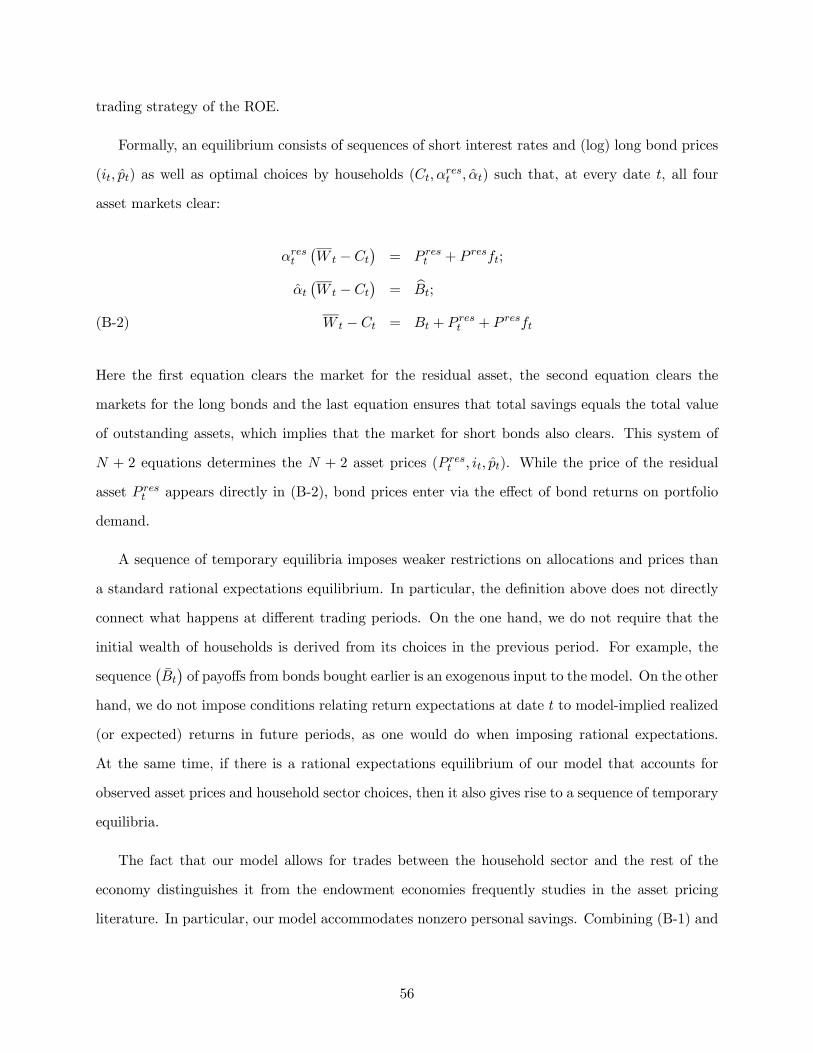
trading strategy of the ROE.

Formally, an equilibrium consists of sequences of short interest rates and (log) long bond prices

(it, pt) as well as optimal choices by households (Ct, αrest , αt) such that, at every date t, all four

asset markets clear:

αrest

¡W t − Ct

¢= P res

t + P resft;

αt¡W t − Ct

¢= bBt;

W t − Ct = Bt + P rest + P resft(B-2)

Here the first equation clears the market for the residual asset, the second equation clears the

markets for the long bonds and the last equation ensures that total savings equals the total value

of outstanding assets, which implies that the market for short bonds also clears. This system of

N + 2 equations determines the N + 2 asset prices (P rest , it, pt). While the price of the residual

asset P rest appears directly in (B-2), bond prices enter via the effect of bond returns on portfolio

demand.

A sequence of temporary equilibria imposes weaker restrictions on allocations and prices than

a standard rational expectations equilibrium. In particular, the definition above does not directly

connect what happens at different trading periods. On the one hand, we do not require that the

initial wealth of households is derived from its choices in the previous period. For example, the

sequence¡Bt

¢of payoffs from bonds bought earlier is an exogenous input to the model. On the other

hand, we do not impose conditions relating return expectations at date t to model-implied realized

(or expected) returns in future periods, as one would do when imposing rational expectations.

At the same time, if there is a rational expectations equilibrium of our model that accounts for

observed asset prices and household sector choices, then it also gives rise to a sequence of temporary

equilibria.

The fact that our model allows for trades between the household sector and the rest of the

economy distinguishes it from the endowment economies frequently studies in the asset pricing

literature. In particular, our model accommodates nonzero personal savings. Combining (B-1) and

56

the last equation in (B-2), we obtain the flow-of-funds identity

(B-3) Ct + P resft +¡Bt − Bt

¢= Dt.

The dividend on the residual asset Dt corresponds to personal income less net personal interest

income. As a result, Dt−Ct is personal savings less net interest. It consists of P resft — net purchases

of all assets other than bonds — and Bt − Bt — net purchases of bonds less net interest. A typical

endowment economy model of the type studied by Lucas (1978) instead assumes that bonds are in

zero net supply and that household net wealth is a claim on future consumption, so that Ct = Dt

and P resft = 0.

57