Boiler Control Systems Engineering Second Edition … · 12 Boiler Control Systems Engineering...

http://bit.ly/29LlCvq

BOILER CONTROLSYSTEMS ENGINEERING,Second Edition

G. F. (Jerry) Gilman

Table of Contents

Chapter 1 — Boiler Fundamentals . . . . . . . . . . . . . . . . . . . . . . . . . . . . . . . . 1Basic Boilers . . . . . . . . . . . . . . . . . . . . . . . . . . . . . . . . . . . . . . . . . . . . . . . . . 1Boiler Components . . . . . . . . . . . . . . . . . . . . . . . . . . . . . . . . . . . . . . . . . . . . 2Furnace . . . . . . . . . . . . . . . . . . . . . . . . . . . . . . . . . . . . . . . . . . . . . . . . . . . . . 2Fans. . . . . . . . . . . . . . . . . . . . . . . . . . . . . . . . . . . . . . . . . . . . . . . . . . . . . . . . 2Windbox . . . . . . . . . . . . . . . . . . . . . . . . . . . . . . . . . . . . . . . . . . . . . . . . . . . . 2Flue Gas Heat Exchangers . . . . . . . . . . . . . . . . . . . . . . . . . . . . . . . . . . . . . . . 2Combustion Air Preheater . . . . . . . . . . . . . . . . . . . . . . . . . . . . . . . . . . . . . . . 5Economizer . . . . . . . . . . . . . . . . . . . . . . . . . . . . . . . . . . . . . . . . . . . . . . . . . 5Superheater . . . . . . . . . . . . . . . . . . . . . . . . . . . . . . . . . . . . . . . . . . . . . . . . . 6Boiler Drums . . . . . . . . . . . . . . . . . . . . . . . . . . . . . . . . . . . . . . . . . . . . . . . . 6Piping and Instrument Diagrams (P&IDs) . . . . . . . . . . . . . . . . . . . . . . . . . . . 7Design Basis Check List. . . . . . . . . . . . . . . . . . . . . . . . . . . . . . . . . . . . . . . . . 8

Chapter 2 — Control of Boilers . . . . . . . . . . . . . . . . . . . . . . . . . . . . . . . . . 11Control Strategies . . . . . . . . . . . . . . . . . . . . . . . . . . . . . . . . . . . . . . . . . . . . 11Bumpless Transfer. . . . . . . . . . . . . . . . . . . . . . . . . . . . . . . . . . . . . . . . . . . . . 11Simple Feedback Control. . . . . . . . . . . . . . . . . . . . . . . . . . . . . . . . . . . . . . . 11Feedforward plus Feedback Control . . . . . . . . . . . . . . . . . . . . . . . . . . . . . . . 12Cascade Control . . . . . . . . . . . . . . . . . . . . . . . . . . . . . . . . . . . . . . . . . . . . . 13Ratio Control . . . . . . . . . . . . . . . . . . . . . . . . . . . . . . . . . . . . . . . . . . . . . . . 14Feedforward Control . . . . . . . . . . . . . . . . . . . . . . . . . . . . . . . . . . . . . . . . . . 14Controller Tuning . . . . . . . . . . . . . . . . . . . . . . . . . . . . . . . . . . . . . . . . . . . . 15Determining Gain, Reset, and Derivative . . . . . . . . . . . . . . . . . . . . . . . . . . . 17Gain vs. Proportional Band (PB) . . . . . . . . . . . . . . . . . . . . . . . . . . . . . . . . . 19Controller Actions . . . . . . . . . . . . . . . . . . . . . . . . . . . . . . . . . . . . . . . . . . . . 19Controller Actions Setup . . . . . . . . . . . . . . . . . . . . . . . . . . . . . . . . . . . . . . . 22The Effects on Tuning . . . . . . . . . . . . . . . . . . . . . . . . . . . . . . . . . . . . . . . . . 22Calibration Effect on Gain . . . . . . . . . . . . . . . . . . . . . . . . . . . . . . . . . . . . . . 22Transmitters . . . . . . . . . . . . . . . . . . . . . . . . . . . . . . . . . . . . . . . . . . . . . . . . 22Redundancy . . . . . . . . . . . . . . . . . . . . . . . . . . . . . . . . . . . . . . . . . . . . . . . . 23Interlock Circuitry. . . . . . . . . . . . . . . . . . . . . . . . . . . . . . . . . . . . . . . . . . . . 23Final Control Elements . . . . . . . . . . . . . . . . . . . . . . . . . . . . . . . . . . . . . . . . 24

Chapter 3 — Furnace Draft . . . . . . . . . . . . . . . . . . . . . . . . . . . . . . . . . . . . . 25Pressure Fired Boilers. . . . . . . . . . . . . . . . . . . . . . . . . . . . . . . . . . . . . . . . . . 25Balanced Draft Boiler Fans. . . . . . . . . . . . . . . . . . . . . . . . . . . . . . . . . . . . . . 26Furnace Pressure Control. . . . . . . . . . . . . . . . . . . . . . . . . . . . . . . . . . . . . . . 26Summer. . . . . . . . . . . . . . . . . . . . . . . . . . . . . . . . . . . . . . . . . . . . . . . . . . . . 30

VII

Gilman front of book.qxd 6/9/2010 11:05 PM Page VII

Chapter 4 — Feedwater . . . . . . . . . . . . . . . . . . . . . . . . . . . . . . . . . . . . . . . . 35Once-Through Boilers . . . . . . . . . . . . . . . . . . . . . . . . . . . . . . . . . . . . . . . . 35Drum Level Feedwater Control . . . . . . . . . . . . . . . . . . . . . . . . . . . . . . . . . . 36Transmitters . . . . . . . . . . . . . . . . . . . . . . . . . . . . . . . . . . . . . . . . . . . . . . . . 41Shrink and Swell . . . . . . . . . . . . . . . . . . . . . . . . . . . . . . . . . . . . . . . . . . . . . 42Single Element Level Control . . . . . . . . . . . . . . . . . . . . . . . . . . . . . . . . . . . 44Two Element Level Control. . . . . . . . . . . . . . . . . . . . . . . . . . . . . . . . . . . . . 44Three Element Level Control . . . . . . . . . . . . . . . . . . . . . . . . . . . . . . . . . . . 48Control System Configuration . . . . . . . . . . . . . . . . . . . . . . . . . . . . . . . . . . . 48Summer . . . . . . . . . . . . . . . . . . . . . . . . . . . . . . . . . . . . . . . . . . . . . . . . . . . 48

Chapter 5 — Coal Fired Boilers . . . . . . . . . . . . . . . . . . . . . . . . . . . . . . . . . 51Pulverized Coal Fired Boilers. . . . . . . . . . . . . . . . . . . . . . . . . . . . . . . . . . . . 51Raw Coal and Feeder . . . . . . . . . . . . . . . . . . . . . . . . . . . . . . . . . . . . . . . . . 54Stoker Boilers . . . . . . . . . . . . . . . . . . . . . . . . . . . . . . . . . . . . . . . . . . . . . . . 56Cyclone Boiler . . . . . . . . . . . . . . . . . . . . . . . . . . . . . . . . . . . . . . . . . . . . . . 56Graphics: Pulverizer Coal Boiler. . . . . . . . . . . . . . . . . . . . . . . . . . . . . . . . . . 59

Chapter 6 — Fuel and Air Control . . . . . . . . . . . . . . . . . . . . . . . . . . . . . . . 67Fuel and Air Control Gas Oil . . . . . . . . . . . . . . . . . . . . . . . . . . . . . . . . . . . 72Fuel and Air Control Characterization . . . . . . . . . . . . . . . . . . . . . . . . . . . . . 74Excess Air to Oxygen . . . . . . . . . . . . . . . . . . . . . . . . . . . . . . . . . . . . . . . . . 76Multiple Fuel Control . . . . . . . . . . . . . . . . . . . . . . . . . . . . . . . . . . . . . . . . . 77Oxygen (O2) Trim Control . . . . . . . . . . . . . . . . . . . . . . . . . . . . . . . . . . . . . 78Multiple Boilers. . . . . . . . . . . . . . . . . . . . . . . . . . . . . . . . . . . . . . . . . . . . . . 80

Chapter 7 — Steam Temperature . . . . . . . . . . . . . . . . . . . . . . . . . . . . . . . . 81Three Element Level Control . . . . . . . . . . . . . . . . . . . . . . . . . . . . . . . . . . . 83

Chapter 8 —Burner Management Systems . . . . . . . . . . . . . . . . . . . . . . . . 91Burner Management System (BMS) Control . . . . . . . . . . . . . . . . . . . . . . . . 91NFPA 85 Code 2007 . . . . . . . . . . . . . . . . . . . . . . . . . . . . . . . . . . . . . . . . . 91Boiler Control and Operating Documentation . . . . . . . . . . . . . . . . . . . . . . . 92Combustion Control . . . . . . . . . . . . . . . . . . . . . . . . . . . . . . . . . . . . . . . . . . 92Purge Control . . . . . . . . . . . . . . . . . . . . . . . . . . . . . . . . . . . . . . . . . . . . . . . 93Requirement for Independence of Control (Hardware/Software) . . . . . . . . . 94Flame Detection . . . . . . . . . . . . . . . . . . . . . . . . . . . . . . . . . . . . . . . . . . . . . 95Flame Monitoring and Tripping System (Multiple Burner Boilers) . . . . . . . . 96Flame Tripping Validation . . . . . . . . . . . . . . . . . . . . . . . . . . . . . . . . . . . . . . . 97Examples of Permissive Starting Logic and Protective Tripping Logic . . . . . 109

VIII

Gilman front of book.qxd 6/9/2010 11:05 PM Page VIII

Chapter 9 — Environment . . . . . . . . . . . . . . . . . . . . . . . . . . . . . . . . . . . . . 111NOx and NOx Control . . . . . . . . . . . . . . . . . . . . . . . . . . . . . . . . . . . . . . . 111Excess Air to Oxygen . . . . . . . . . . . . . . . . . . . . . . . . . . . . . . . . . . . . . . . . 113Boiler Efficiency Computations . . . . . . . . . . . . . . . . . . . . . . . . . . . . . . . . . 115Input/Output Example . . . . . . . . . . . . . . . . . . . . . . . . . . . . . . . . . . . . . . . 115

Chapter 10 — Control Valve Sizing. . . . . . . . . . . . . . . . . . . . . . . . . . . . . . 117Valve Characteristics. . . . . . . . . . . . . . . . . . . . . . . . . . . . . . . . . . . . . . . . . . 117Valve Characteristic Graph . . . . . . . . . . . . . . . . . . . . . . . . . . . . . . . . . . . . . 118Recommended Velocities . . . . . . . . . . . . . . . . . . . . . . . . . . . . . . . . . . . . . . 118Valve Sizing for Different Control Media . . . . . . . . . . . . . . . . . . . . . . . . . . 119Control Valve Sizing Calculations . . . . . . . . . . . . . . . . . . . . . . . . . . . . . . . . 119Gas Valve Sizing . . . . . . . . . . . . . . . . . . . . . . . . . . . . . . . . . . . . . . . . . . . . . 120

Chapter 11 — Steam Temperature Control . . . . . . . . . . . . . . . . . . . . . . . 123Purpose . . . . . . . . . . . . . . . . . . . . . . . . . . . . . . . . . . . . . . . . . . . . . . . . . . . 123Introduction . . . . . . . . . . . . . . . . . . . . . . . . . . . . . . . . . . . . . . . . . . . . . . . 123Principles and Methods of Transient Superheat Steam . . . . . . . . . . . . . . . . 124

Temperature ControlNOx Control. . . . . . . . . . . . . . . . . . . . . . . . . . . . . . . . . . . . . . . . . . . . . . . 126Redundancy . . . . . . . . . . . . . . . . . . . . . . . . . . . . . . . . . . . . . . . . . . . . . . . 126Reset Windup Prevention . . . . . . . . . . . . . . . . . . . . . . . . . . . . . . . . . . . . . 126Advanced Steam Temperature Control . . . . . . . . . . . . . . . . . . . . . . . . . . . . 127

Acronyms . . . . . . . . . . . . . . . . . . . . . . . . . . . . . . . . . . . . . . . . . . . . . . . . . . . 129

Appendix A. . . . . . . . . . . . . . . . . . . . . . . . . . . . . . . . . . . . . . . . . . . . . . . . . . 131

Appendix B . . . . . . . . . . . . . . . . . . . . . . . . . . . . . . . . . . . . . . . . . . . . . . . . . 141

Appendix C . . . . . . . . . . . . . . . . . . . . . . . . . . . . . . . . . . . . . . . . . . . . . . . . . 179

Appendix D . . . . . . . . . . . . . . . . . . . . . . . . . . . . . . . . . . . . . . . . . . . . . . . . . 181

Bibliography . . . . . . . . . . . . . . . . . . . . . . . . . . . . . . . . . . . . . . . . . . . . . . . . . 187

References. . . . . . . . . . . . . . . . . . . . . . . . . . . . . . . . . . . . . . . . . . . . . . . . . . . 189

Kraft Pulp Mill . . . . . . . . . . . . . . . . . . . . . . . . . . . . . . . . . . . . . . . . . . . . . . . 195

Index . . . . . . . . . . . . . . . . . . . . . . . . . . . . . . . . . . . . . . . . . . . . . . . . . . . . . . . 197

IX

Gilman front of book.qxd 6/9/2010 11:05 PM Page IX

CHAPTER 2

Control of Boilers

Control Strategies

There are basically five fundamental control strategies that are used in process control.They are:simple feedback control, feedforward plus feedback control, cascade control, ratio control, andfeedforward control. In the control of boilers, all five of the fundamental control strategies areused. Many companies show all controllers on drawings as PID controllers. This is becausevendor algorithms/function blocks for control are defined as PID controllers. Most controlloops are PI only, therefore that format is used in this book.

Bumpless Transfer

The NFPA 85 Code requires bumpless transfer from manual to automatic.Before the devel-opment of the DCS (distributed control systems or digital control systems) and electronicsystems, it was the responsibility of the operator to line up the set point and the processvariable before transferring to automatic control.These systems have the capability of theset point tracking the process variable so they are aligned when control is transferred toautomatic control.

Simple Feedback Control

With simple feedback control, changes in the primary variable feedback to a control function,as shown in Figure 2-1.The process variable is compared to the set point of the controller.Thedifferential between the set point and process variable generates an output signal to the manip-ulated variable and adjusts the variable to bring it back to set point. The function can beproportional-plus-integral (as shown), proportion-only, proportional-plus-derivative, integral-only, or proportional-plus-integral-plus-derivative.

In all these cases, the controller includes an error detector function, which measures the errorbetween the primary variable and the set point. Other terms are used such as process variableor measured variable.The controller output is determined by a combination or summation of the effects of the different control action capabilities that are built into the controller.This can be gain, reset, derivative, or any combination of the three.These are the proportionalor gain multiplication of the error magnitude, the difference between the measured amountand the set point, the integral action based on incremental time away from set point multi-plied by error magnitude, and the derivative or rate of change of the measured variable.

Control of Boilers 11

Gilman chp2.qxd 6/14/2010 9:27 PM Page 11


Derivative action is not represented in the functional diagram/symbol drawing examples,although it may be used. Derivative action should only be used when there is dead time or aslow responding process such as temperature control.A change in the controller output changesthe manipulated variable, which through action of the process, changes the process outputselected as the primary variable.The manipulated variable may also be referred to as the processvariable. For drum level control, the manipulated variable is the water flow. On draft control,the manipulated variable is typically the ID fan vane or damper and may be ID fan speed con-trol or a combination of vane or damper and speed.

More detail on how proportional, integral, and derivative action function is covered in con-troller tuning.

Feedforward plus Feedback Control

In feedforward-plus-feedback control, a secondary variable that has a predictable relationshipwith the manipulated variable is connected (Figure 2-2). In this case, a change in the secondaryvariable causes the manipulated variable to change in anticipation of a change in the primaryvariable.This reduces the magnitude of the primary variable change due to the more timelycontrol action that originates from the secondary variable.The feedback portion of the loopcontains the set point and can contain any of the controller functions of the basic feedbackloop.The feedforward gain is adjustable.

Basically, the feedforward portion of the control loop minimizes upsets and keeps the processat the desired set point.

12 Boiler Control Systems Engineering

Figure 2-1 Simple feedback control.Note: See Reference section for explanation of functional diagram/symbols.


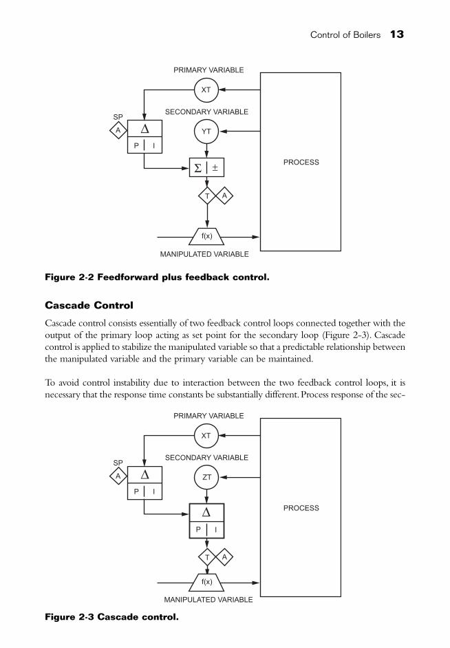
Cascade Control

Cascade control consists essentially of two feedback control loops connected together with theoutput of the primary loop acting as set point for the secondary loop (Figure 2-3). Cascadecontrol is applied to stabilize the manipulated variable so that a predictable relationship betweenthe manipulated variable and the primary variable can be maintained.

To avoid control instability due to interaction between the two feedback control loops, it isnecessary that the response time constants be substantially different.Process response of the sec-


Figure 2-2 Feedforward plus feedback control.

Figure 2-3 Cascade control.


ondary control loop should be the faster of the two.A general rule is that the time constant ofthe primary loop process response should be a minimum of 5 to 10 times that of the secondaryloop.The longer time constant of the primary loop indicates a much slower response. Becauseof this, a normal application would be temperature control (a normally slow loop) cascadingonto flow control (a normally fast loop).Other suitable candidates for cascade control are tem-perature cascading onto pressure control and level control cascading onto flow control.

Ratio Control

Ratio control consists of a feedback controller whose set point is in direct proportion to anuncontrolled variable (Figure 2-4).The operator of the process can set the proportional rela-tionship, or another controller, or a feedforward signal can automatically adjust it.When boilersburn multiple fuels, air requirements for the different fuels may vary. Ratio control is used toratio the quantity of air required for different fuels.

As shown, the mathematical function is a multiplier. If the ratio is set, the set point of the con-trolled variable changes in direct proportion to changes in the uncontrolled variable. If themultiplication is changed, the direct proportional relationship, or ratio between the controlledand the uncontrolled variable, is changed.

Most boiler control applications will consist of an overall control system in an interconnectedmatrix of the five types of control.

Feedforward Control

Feedforward control is used in a number of configurations to improve process control. In feed-forward control, a measured variable is used to detect a process change in the system. The


Figure 2-4 Ratio control.


measured variable sends this information to a feedforward controller.The feedforward controllerdetermines the required change in the manipulated variable, so that when the effect of the changeis combined with the change in the manipulated variable, no change occurs in the controlledvariable. This perfect correction is difficult to accomplish. Feedforward control has some significant problems. The configuration of feedforward control assumes that the changes areknown in advance, that the changes will have transmitters associated with them, and that noimportant undetected changes will occur. Steam flow is used as a feedforward signal for the setpoint of an O2 analyzer, or the signal from a fuel flow can be used to set a fuel air ratio (Figure5-3 in Chapter 5). Feedforward can be used to add derivative to increase pulverizer coal feed.

Controller Tuning

There are a number of procedures for tuning controllers.There is Default Tuning, S.W.A.G.tuning, Ziegler Nichols, Lambda, and self tuning. Some startup engineers still use the trial anderror or S.W.A.G. method.

Self-tuning controller algorithms are now available for insertion into control systems. Such con-trollers automatically compensate the controller tuning as process or boiler conditions change.Adaptive tuning can also be implemented from load or some other variable of the process.

“Lambda tuning was originated in the synthesis design method whereby the controller mustcancel out the process dynamics. In more technical words, given the transfer functions of thecomponents of a feedback loop, synthesize the controller required to produce a specific closed-loop response (loop in automatic).The simplest achievable closed-loop response is a first-orderlag.This response was originally proposed by Dahlin (1968), who defined the tuning parameterwith the Greek letter Lambda, to signify the time constant of the control loop in automatic,hence the name Lambda Tuning.Lambda Tuning produces a first order,non-oscillatory responseto a set point change.This is done by selecting the desired time constant on automatic. Loopstuned using Lambda Tuning will minimize (or eliminate) over-shoot, have great flexibility, andpresent repeatable results.This method is becoming more popular as more uniform products arerequired, minimum variability is demanded, and stable processes are needed.”1

To demonstrate the various tuning modes the Ziegler Nichols method is used. In 1942,Zieglerand Nichols were the first to propose a standard method for tuning feedback controllers.Afterstudying numerous processes, they arrived at a series of equations that can be used for calcu-lating the gain, reset, and derivative values for feedback control loops. They developed twomethods. One is referred to as the ultimate method because it requires the determination ofthe ultimate gain (sensitivity) and the ultimate period for the control loop.The ultimate gainis the maximum allowable value of gain for a controller with only a proportional mode inoperation for which the closed loop system shows a stable sine wave response to a disturbance.

The second method developed by Ziegler and Nichols for tuning control loops was based ondata from the process reaction curve for the system under control.The process reaction curveis simply the reaction of the process to a step change in the input signal.This process curve isthe reaction of all components in the control system (excluding the controller) to a step changeto the process.


1 Tom Dorsch,“Lambda Tuning:An Alternative to Ziegler Nichols,” December 1997: Fisher Controls.


The ultimate method is also referred to as the quarter decay tuning (see Figure 2-5 and Table2-1 for the equations).This method requires defining the Su and the Pu (Figure 2-6). Su is ulti-mate sensitivity and is the gain or proportional band that creates a continuous sine wave,steady-state output as indicated on the center graph in Figure 2-6.This is determined with thereset/integral turned off. Pu is the ultimate period or time between the peaks of the steady-statesine wave in Figure 2-6.

The ultimate method is used in the examples because it is easy to understand and demonstratesthe difference between proportional/gain, reset/integral, and derivative control by using PC-ControLAB 3,a software training program developed by Harold Wade Associates and sold by ISA.The top diagram in Figure 2-6 demonstrates an unstable response. In this diagram the outputvariations become larger and larger. The bottom diagram demonstrates dampened response. Inthis diagram the outputs become smaller and smaller.With this method there is overshoot. Insome cases, it is important to tune the system so that there is no overshoot.

The center diagram demonstrates a stable response. From this diagram we can determine theSu and the Pu. In these equations, gain is used and the integral is in minutes/repeat. Some ven-dors use repeats/minute instead of minutes/repeat, or proportional band, instead of gain.

For any feedback control system, if the loop is closed (and the controller is on automatic), onecan increase the controller gain, during which time the loop will tend to oscillate more andmore. If the gain is further increased, continuous cycling, or oscillation in the controller vari-able, will be observable.This is the maximum gain at which the system can be operated beforeit becomes unstable; therefore, this is the ultimate gain.The period of these sustained oscilla-tions is called the ultimate period. If the gain is increased further still, the system will becomeunstable.These three situations are illustrated in Figure 2-6.


Figure 2-5 Ziegler Nichols tuning.



Determining Gain, Reset, and Derivative

To determine the ultimate gain and the ultimate period, remove the reset and derivative actionfrom the controller by setting the derivative time to zero and the reset time to infinity, or turnthe reset off. PC-ControLAB 3 provides the ability to turn off the reset by going to tuneoptions and turning off reset.

With the controller in the automatic mode, the loop closed, and the gain set at 12, an upset isimposed on the control loop and the response observed.The easiest way to impose an upset isto change the set point by a small amount. If the response curve produced does not dampenout and is unstable (top of Figure 2-6 - unstable response), the gain is too high.

With the gain set to 3, an upset is created. If the response curve dampens out (bottom of Figure 2-6 - dampened response), the gain is too low. The gain was increased and upsets repeateduntil a stable response was obtained.


Table 2-1 Tuning terms/equations

Terms are:

Equations are:Proportional onlyKc = 0.5 Su

Proportional-Plus-ResetKc = 0.45 SuTi = Pu/1.2 min/rpt

Proportional-Plus-DerivativeKc = 0.6 SuTd = Pu/8

Proportional-Plus-Reset-Plus-DerivativeKc = 0.6 SuTi = 0.5 Pu min/rptTd = Pu/8

Using the equations Su = 9 and Pu = 7.5 minutesfrom Figure 2-6.

Proportional only Figure 2-6 aKc = 0.5 Su 0.5 x 9 = 4.5 gain

Proportional-plus-reset Figure 2-6 bKc = 0.45 Su 0.45 x 9 = 4.05 gainTi = Pu/1.2 min/rpt 7.5 / 1.2 = 6.25 reset

Proportional-Plus-Reset-Plus-Derivative Figure 2-6 cKc = 0.6 Su 0.6 x 9 = 5.4 gainTi = 0.5 Pu min/rpt 0.5 x 7.5 = 3.75 resetTd = Pu/8 7.5 / 8 = 0.94 derivative

Kc = gainTi = integral, reset (Time integral) Td = derivative (Time)

Pu = ultimate periodSu = ultimate sensitivity


When a stable response is obtained, the values of the ultimate gain (Su) and the ultimate period(Pu) of the associated response curve should be noted.The ultimate period is determined bythe time period between successive peaks on the stable response curve.The ultimate gain (alsocalled the ultimate sensitivity or Su) is the gain setting of the controller when a stable responseis reached (center of Figure 2-6 - stable response).

Using PC-ControLAB 3, the stable response is achieved with a gain of 9, and the time from peak to peak is approximately 7.5 minutes.The 7.5 minutes is the peak to peak time onFigure 2-7.The cycle is generated with a gain of 9 and no reset (reset turned off).


Figure 2-6 Typical control system responses.


Gain vs. Proportional Band (PB)

Gain and proportional band are used as tuning terms. Gain is the reciprocal of proportionalband. Proportional band (PB) is in percent.

Prop Band = 100 / Gain Gain = 100 / Prop Band

Examples: If Gain is 2, PB = ½ = 0.5 X 100 = 50% PB or 100% / 2 = 50%If Gain is 0.5, PB = 1 = 2 X 100/0.5 = 200% PB or 100% / 0.5 = 200%

Repeats per minute vs. minutes per repeat:

Integral Action is minutes per repeat or repeats per minute. Repeats per minute is thereciprocal of minutes per repeat.

Example: 0.5 Min/Repeat = 1/0.5 = 2 Repeats/Min

Figure 2-7 demonstrates a typical output variable.

Figure 2-7 Typical output variable.Note: Only a small output cycle is required to determine the Su and Pu values.

Controller Actions

Gain/Proportional ActionWhen gain/proportional control only is used, there is a one-time step change based on devi-ation from set point. A feedback controller with gain/proportional control only, may notstabilize the set point (Figure 2-8). Note the difference between the process variable (PV) andset point (SP). For gain/proportional only control, the gain is 4.5 (Table 2-1).



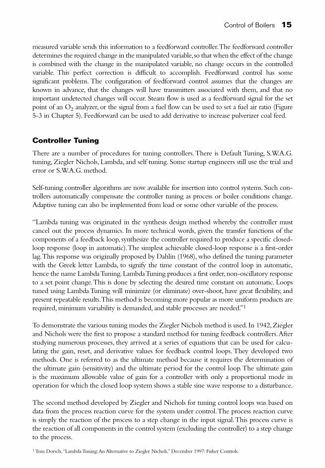
Figure 2-8 Deviation between setpoint and process variable.

Integral/Reset ActionIntegral action is time-based change in minutes and repeats the gain change until the loop stabilizes at set point.The tuning setting is in repeats per minute or minutes per repeat. Notein Figure 2-9 with gain/proportional and integral/reset action, the measurement lines out atset point in approximately 30 minutes. Also note the recovery on the second cycle is onequarter of the first cycle. For gain/proportional plus reset control, the gain is 4.05 and reset is6.25 (Table 2-1).

Figure 2-9 Upset and return to recovery with reset.




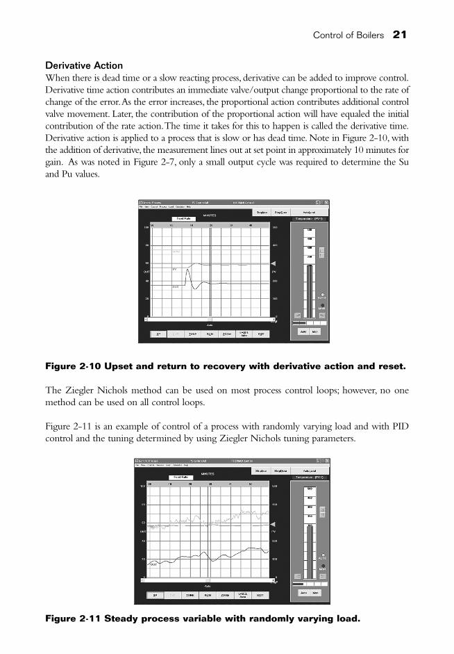
Derivative ActionWhen there is dead time or a slow reacting process, derivative can be added to improve control.Derivative time action contributes an immediate valve/output change proportional to the rate ofchange of the error.As the error increases, the proportional action contributes additional controlvalve movement. Later, the contribution of the proportional action will have equaled the initialcontribution of the rate action.The time it takes for this to happen is called the derivative time.Derivative action is applied to a process that is slow or has dead time. Note in Figure 2-10, withthe addition of derivative, the measurement lines out at set point in approximately 10 minutes forgain. As was noted in Figure 2-7, only a small output cycle was required to determine the Suand Pu values.

Figure 2-10 Upset and return to recovery with derivative action and reset.

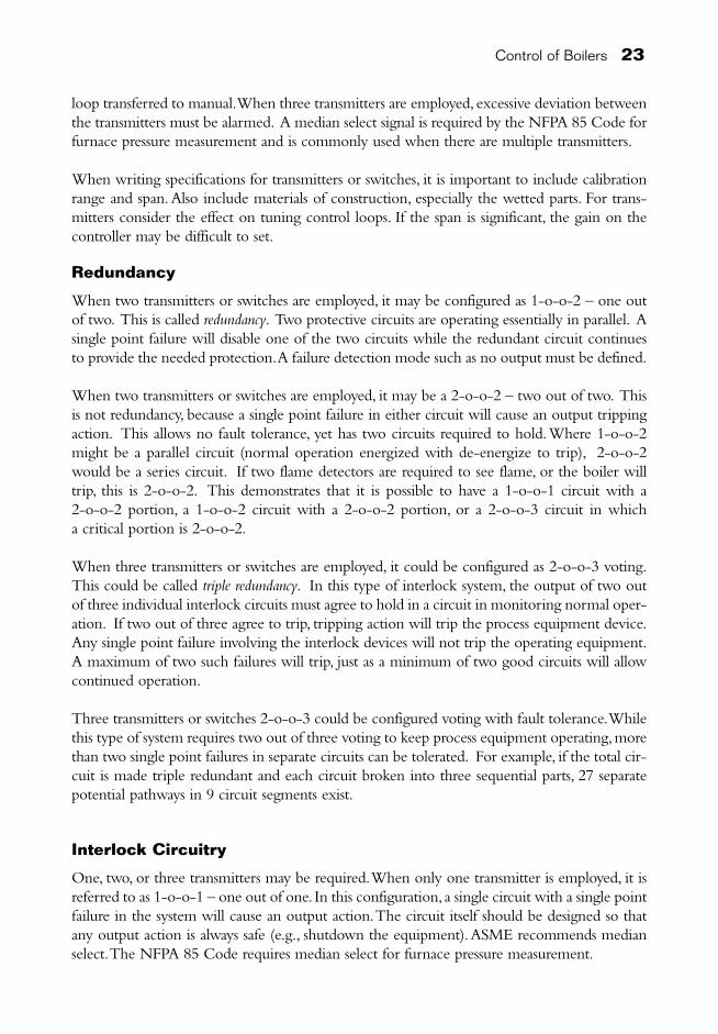
The Ziegler Nichols method can be used on most process control loops; however, no onemethod can be used on all control loops.

Figure 2-11 is an example of control of a process with randomly varying load and with PIDcontrol and the tuning determined by using Ziegler Nichols tuning parameters.

Figure 2-11 Steady process variable with randomly varying load.



Controller Actions Setup

There are many different functions required in design and configuration and/or programminga control system. Controller functions need to be determined. Controller functions can bedirect or reverse acting.A direct acting controller output increases as the PV (Process Variable)increases, and a reverse acting controller output decreases as the PV increases. If the controlsystem is programmable, the systems engineer must make the selection.The failure mode of thecontrol valve or damper determines whether the controller is a direct or reverse acting con-troller.Units of measurement are in percent or engineering units.When we think of the variouscontrol signals such as the process variable or set points, we can define them as a percentage orassign engineering units.

The Effects on Tuning

There are numerous things that affect the tuning of control loops. Some examples are: reactiontime of process, process noise (furnace pressure, air flow), calibration of transmitter (span of thetransmitter), linearity of process (pH loop), linearity of final element, speed of response of finalelement (valves, dampers), valve sizing and valve hysteresis.The addition of a valve positionercan improve control by providing valve position repeatability for a specific input.

Temperature control would be an example of a slow responding process. Flow control wouldbe an example of a fast responding process.

Calibration Effect on Gain

Example: Span of transmitter

0-2000 psi 4-20 ma = 125 psi/ma1000 to 2000 psi 4-20 ma = 62.5 psi/ma

Note, the span is one number and calibration range is two numbers.

Using engineering units in this example, the span of 0-2000 is two times that of the span 1000-2000. Therefore, the gain would be two times greater than when calibrated with a span of0-2000 psi.This is a common problem particularly on high pressure boilers.With a wide span,a control output may cycle and yet the process appears to be steady.

There is no one method of control tuning that is best for all process loops. Different types ofprocesses, control valves or dampers, vendor control algorithms or function blocks can makethis impractical.

Transmitters

Each control loop should be reviewed by a risk analysis to determine if a redundant transmitteror switch is required. Field transmitter or switch device redundancy should be provided to theextent necessary to achieve desired system reliability.When two transmitters or switches areemployed, excessive deviation between the devices must be alarmed and the associated control



loop transferred to manual.When three transmitters are employed, excessive deviation betweenthe transmitters must be alarmed. A median select signal is required by the NFPA 85 Code forfurnace pressure measurement and is commonly used when there are multiple transmitters.

When writing specifications for transmitters or switches, it is important to include calibrationrange and span. Also include materials of construction, especially the wetted parts. For trans-mitters consider the effect on tuning control loops. If the span is significant, the gain on thecontroller may be difficult to set.

Redundancy

When two transmitters or switches are employed, it may be configured as 1-o-o-2 – one outof two. This is called redundancy. Two protective circuits are operating essentially in parallel. Asingle point failure will disable one of the two circuits while the redundant circuit continuesto provide the needed protection.A failure detection mode such as no output must be defined.

When two transmitters or switches are employed, it may be a 2-o-o-2 – two out of two. Thisis not redundancy, because a single point failure in either circuit will cause an output trippingaction. This allows no fault tolerance, yet has two circuits required to hold.Where 1-o-o-2might be a parallel circuit (normal operation energized with de-energize to trip), 2-o-o-2would be a series circuit. If two flame detectors are required to see flame, or the boiler willtrip, this is 2-o-o-2. This demonstrates that it is possible to have a 1-o-o-1 circuit with a 2-o-o-2 portion, a 1-o-o-2 circuit with a 2-o-o-2 portion, or a 2-o-o-3 circuit in which a critical portion is 2-o-o-2.

When three transmitters or switches are employed, it could be configured as 2-o-o-3 voting.This could be called triple redundancy. In this type of interlock system, the output of two outof three individual interlock circuits must agree to hold in a circuit in monitoring normal oper-ation. If two out of three agree to trip, tripping action will trip the process equipment device.Any single point failure involving the interlock devices will not trip the operating equipment.A maximum of two such failures will trip, just as a minimum of two good circuits will allowcontinued operation.

Three transmitters or switches 2-o-o-3 could be configured voting with fault tolerance.Whilethis type of system requires two out of three voting to keep process equipment operating,morethan two single point failures in separate circuits can be tolerated. For example, if the total cir-cuit is made triple redundant and each circuit broken into three sequential parts, 27 separatepotential pathways in 9 circuit segments exist.

Interlock Circuitry

One, two, or three transmitters may be required.When only one transmitter is employed, it isreferred to as 1-o-o-1 – one out of one. In this configuration, a single circuit with a single pointfailure in the system will cause an output action.The circuit itself should be designed so thatany output action is always safe (e.g., shutdown the equipment).ASME recommends medianselect.The NFPA 85 Code requires median select for furnace pressure measurement.



Final Control Elements

All final control elements are to be designed to fail safe on loss of demand signal or motivepower, i.e., open, close, or lock in place.The fail safe position must be determined by the userand based upon the specific application.




Boiler Control Systems Engineering Second Edition … · 12 Boiler Control Systems Engineering...

Documents

Transcript of Boiler Control Systems Engineering Second Edition … · 12 Boiler Control Systems Engineering...