This Provisional PDF corresponds to the article as it appeared upon acceptance. Fully formattedPDF and full text (HTML) versions will be made available soon.

A nomogram for P values

BMC Medical Research Methodology 2010, 10:21 doi:10.1186/1471-2288-10-21

Leonhard Held (leonhard.held@ifspm.uzh.ch)

ISSN 1471-2288

Article type Research article

Submission date 9 December 2009

Acceptance date 16 March 2010

Publication date 16 March 2010

Article URL http://www.biomedcentral.com/1471-2288/10/21

Like all articles in BMC journals, this peer-reviewed article was published immediately uponacceptance. It can be downloaded, printed and distributed freely for any purposes (see copyright

notice below).

Articles in BMC journals are listed in PubMed and archived at PubMed Central.

For information about publishing your research in BMC journals or any BioMed Central journal, go to

http://www.biomedcentral.com/info/authors/

BMC Medical ResearchMethodology

© 2010 Held , licensee BioMed Central Ltd.This is an open access article distributed under the terms of the Creative Commons Attribution License (http://creativecommons.org/licenses/by/2.0),

which permits unrestricted use, distribution, and reproduction in any medium, provided the original work is properly cited.

A nomogram for P values

Leonhard Held∗1

1Biostatistics Unit, Institute of Social and Preventive Medicine, University of Zurich, Hirschengraben 84, 8001 Zurich, Switzerland

Email: Leonhard Held∗- leonhard.held@ifspm.uzh.ch;

∗Corresponding author

1

Abstract

Background: P values are the most commonly used tool to measure evidence against a hypothesis. Several

attempts have been made to transform P values to minimum Bayes factors and minimum posterior probabilities

of the hypothesis under consideration. However, the acceptance of such calibrations in clinical fields is low due

to inexperience in interpreting Bayes factors and the need to specify a prior probability to derive a lower bound

on the posterior probability.

Methods: I propose a graphical approach which easily translates any prior probability and P value to minimum

posterior probabilities. The approach allows to visually inspect the dependence of the minimum posterior

probability on the prior probability of the null hypothesis. Likewise, the tool can be used to read off, for fixed

posterior probability, the maximum prior probability compatible with a given P value. The maximum P value

compatible with a given prior and posterior probability is also available.

Results: Use of the nomogram is illustrated based on results from a randomized trial for lung cancer patients

comparing a new radiotherapy technique with conventional radiotherapy.

Conclusion: The graphical device proposed in this paper will enhance the understanding of P values as measures

of evidence among non-specialists.

Background

P values are the most commonly used tool to measure evidence against a hypothesis [1]. The P value is

defined as the probability, under the assumption of no effect (the null hypothesis H0), of obtaining a result

equal to or more extreme than what was actually observed. The complexity of this definition has led to

widespread misinterpretations and criticisms [2–5]. Indeed, P values are often misinterpreted (a) as the

probability of obtaining the observed data under the assumption of no real effect, (b) as an “observed”

type-I error rate, (c) as the false discovery rate, i.e. the probability that a significant finding is “false

positive”, and (d) as the (posterior) probability of the null hypothesis [6].

The latter misinterpretation has given rise to interesting work on the connection between P values and

(posterior) probabilities of the null hypothesis. Within a Bayesian framework, the posterior probability is a

2

function of the prior probability and the so-called Bayes factor, which summarizes the evidence against the

null hypothesis.

Several attempts have been made to transform P values to lower bounds on the Bayes factor and the

resulting posterior probability of the null hypothesis [7–11]. In this context Bayes factors are usually

oriented as P values such that smaller values provide stronger evidence against the null hypothesis. These

techniques calibrate P values such that an interpretation as minimum Bayes factor or minimum posterior

probability is justified. Although the different approaches do not result in identical calibration scales, a

universal finding is that the evidence against a simple null hypothesis is by far not as strong as the P value

might suggest.

However, the acceptance of calibrated P values in clinical fields is low. Minimum Bayes factors have the

advantage that they do not depend on the prior probability of the null hypothesis [9], but their

interpretation requires an intuitive understanding of odds, similar to likelihood ratios in diagnostic

studies [12]. Clinicians, however, prefer to think in terms of probabilities. The calculation of the minimum

posterior probability, on the other hand, requires to decide on a prior probability of the null hypothesis.

Fixing a prior probability may be difficult for the clinician, who would perhaps prefer to investigate - for a

given P value - the dependence of the (minimum) posterior probability of the null hypothesis on the prior

probability.

In this paper I propose a graphical approach, which easily translates any prior probability and P value into

minimum posterior probabilities. Likewise, the tool can be used to derive, for fixed posterior probability,

the maximum prior probability compatible with a given P value. The maximum P value in accordance

with a given prior and posterior probability can be also read off. The approach is inspired by the Fagan

nomogram [13] used to derive the post-test probability in diagnostic tests [12]. It will enhance the

understanding and facilitate the interpretation of P values as measures of evidence against the null

hypothesis among non-specialists.

MethodsCalibration of P values

In a seminal paper, Edwards, Lindman and Savage [7] (ELS) studied the relationship between P values and

minimum Bayes factors in several settings. Of particular interest is the case where a test statistic is normal

distributed with unknown mean µ. A simple null hypothesis H0 corresponds to a particular mean value

µ = µ0. Calculation of the Bayes factor requires fixing a prior density for µ under the alternative

3

hypothesis H1 : µ 6= µ0.

This scenario reflects, at least approximately, many of the statistical procedures found in medical journals.

The minimum Bayes factor turns out to be

BF = exp(−0.5z2),

here z is the z-value, i.e. the test statistic which has given rise to the observed P value. This lower bound

can be derived using the fact that the Bayes factor is minimized if the alternative hypothesis has all its

prior density at one particular value of µ supported most by the data (the Maximum Likelihood estimate).

Because this point is always on one side of the null hypothesis, ELS suggested to use a z-value based on a

one-tailed rather than a two-tailed significance test. A two-tailed test, which leads to slightly larger values

of z and to slightly smaller values of BF has also been suggested [9].

For a fixed prior probability q, say, of the null hypothesis, the minimum Bayes factor BF can easily be

transformed into a lower bound on the posterior probability of the null hypothesis based on Bayes’ theorem:

Minimum Posterior Probability =

(1 +

(BF · q1− q

)−1)−1

. (1)

The first row in Table 1 gives this lower bound for q = 50% and P values of 0.05, 0.01 and 0.001,

respectively, using the ELS approach. A striking feature is that the lower bound for the posterior

probability is considerably larger than the corresponding P value.

The ELS approach has been refined by Berger and Sellke [8] (BS). They derived lower bounds for the

Bayes factor under more realistic families of prior distributions for µ under the alternative hypothesis. In

particular, they considered (1) symmetric prior distributions, (2) unimodal and symmetric prior

distributions, and (3) normal prior distributions, all centered at µ0. As one would expect, the

corresponding lower bounds on the posterior probability of H0 increase with increasing restrictions on the

prior family for µ, as can be seen in Table 1.

Perhaps the simplest and most intuitive calibration has been suggested by Sellke, Bayarri and Berger [10]

(SBB). They use the fact that a P value is (under suitable regularity conditions) uniformly distributed if

H0 is true. Under the alternative hypothesis smaller P values are more likely than larger P values, i.e. the

density of the P value is monotonically decreasing. A flexible class of decreasing densities on the unit

interval is provided by specific beta densities with one unknown parameter. The minimum Bayes factor is

then

BF =

{−e p log p if p < 1/e1 otherwise.

4

Here p is the observed P value and e = exp(1) ≈ 2.718 is Euler’s constant. The resulting lower bounds on

the posterior probability of the null hypothesis are very similar to those obtained using the BS approach

with a unimodal prior density for µ, as can be seen from Table 1. Note that the SBB bounds hold in a more

general setting without the assumption of a beta distributed P value under the alternative hypothesis [10].

More recently, minimum Bayes factors for χ2-distributed test statistics have been studied [11]. Such test

statistics have an additional parameter, the degrees-of-freedom ν, which depends on the specific type of

test applied. The following lower bound on the Bayes factor has been derived:

BF =

{ (νx

)−ν/2exp

(−x−ν2

)for x > ν

1 otherwise.

Here, x is the value of the χ2-test statistic which has given rise to the observed P value. It can be easily

shown that BF decreases with increasing degrees-of-freedom. Perhaps more interestingly, BF is equal to the

BS lower bound for normal priors for ν = 1, equals the SBB lower bound for ν = 2, and is equal to the ELS

lower bound for ν →∞. This illustrates that the range of lower bounds on the posterior probability given

in Table 1 reflects a large variety of different tests and scenarios.

A nomogram for P values

The apparent complexity of the formulae presented in the previous section may be one of the reasons why

the proposed calibration of P values has not entered routine scientific research. I therefore suggest to adapt

a graphical device, originally developed for diagnostic tests [13], to the setting outlined above. The original

Fagan nomogram allows to visually determine the post-test probability for a given pre-test probability and

a likelihood ratio in a diagnostic test framework [12]. The likelihood ratio is a function of sensitivity,

specificity and the actual result of the diagnostic test considered. The likelihood ratio is a specific form of a

Bayes factor where both hypotheses under consideration (either the patient has the disease or not) are

simple and no additional prior assumptions have to be made.

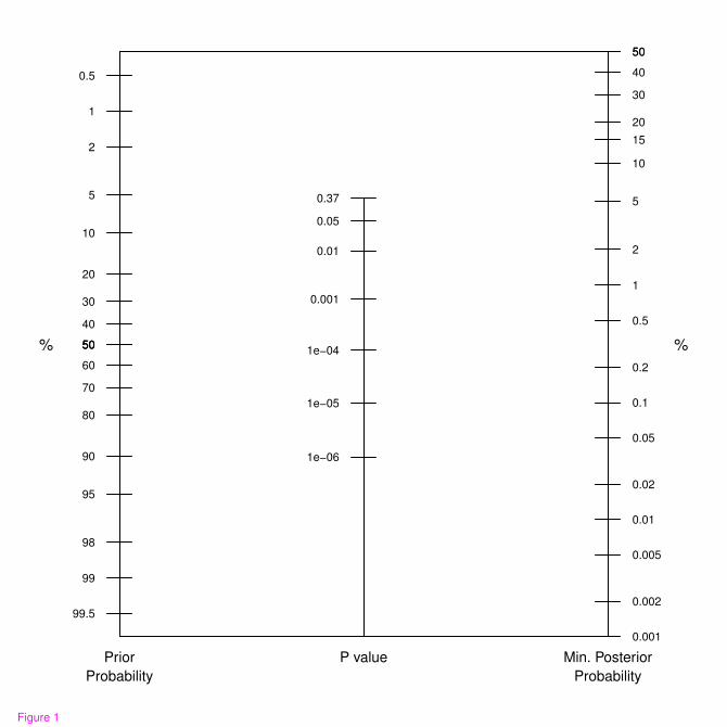
The proposed graphical device is shown in Figure 1. The prior probability for the null hypothesis is located

on the first axis and joined to the observed P value on the second axis. The minimum posterior probability

is then read off the third axis. The P value scaling on the second axis is based on the SBB calibration. Of

course, any other of the calibrations discussed in the previous section could have been used, but the SBB

approach seems particularly suitable since it is not designed for a specific test statistic (normal or χ2) but

is derived in a more general setting.

Note that there are some notable differences compared with the original Fagan nomogram. First, the

5

likelihood ratio is replaced with the P value. Secondly, only P values smaller than 1/e ≈ 0.37 are

considered since BF is unity for larger P values, where there is lack of evidence against the null hypothesis.

Therefore the prior probability scale on the left-hand side of the plot is not identical to the posterior

probability scale on the right-hand side of the plot. This reflects the fact that P values are asymmetric

measures of evidence, they quantify the evidence against the null hypothesis, but they do not quantify the

evidence in favour of the null hypothesis. This is different in the Fagan nomogram, where likelihood ratios

can be both larger and smaller than unity. Finally, the third axis gives not an exact value for the posterior

probability of the null hypothesis but only the minimum posterior probability.

Results

The proposed nomogram can be used in three different ways, as will be illustrated by the following

example. In 1986 a new radiotherapy technique called CHART was introduced. Promising pilot studies led

the UK Medical Research Council to instigate a large randomized trial for lung cancer patients. The

objective of the study was to estimate the change in survival when given CHART compared with

conventional radiotherapy.

Before the trial a q = 10% prior chance that CHART would offer no survival benefit at all was elicited from

11 clinicians [5]. At the end of the trial a clinically important and statistically significant difference in

survival was found (9% improvement in 2 year survival, 95% CI: 3-15%, Two-sided P value = 0.3%,

i.e. 0.003) [14]. We can now easily read off the lower bound of around 0.5% for the posterior probability of

the null hypothesis (green line in Figure 2).

Due to the relatively small prior probability, the minimum posterior probability of the null hypothesis is in

this example numerically quite close to the P value. This will be different for larger prior probabilities. For

example, for q = 50% we obtain a minimum posterior probability of no survival benefit of around 4.5% (red

line). For q = 90% the minimum posterior probability is 29.9% (blue line).

There are two other ways how to use the nomogram, solving for either the prior probability or the P value.

For example, to obtain a posterior probability of 0.3% with a P value of 0.3%, the prior probability must

be 6% or smaller, as can be read off from the red line in Figure 3. Alternatively, one might be interested in

the maximum P value that is compatible with a reduction of the probability of the null hypothesis from

50% a priori to 0.3% a posteriori, say. Figure 3 indicates (green line) that we need a P value of 0.014%

(0.00014) or smaller to achieve this, more than one order of magnitude smaller than the targeted posterior

probability of 0.3%.

6

Discussion

The Fagan nomogram [12] is widely used in the context of diagnostic tests and I hope that the proposed

nomogram for P values will reach similar popularity. It visually transforms P values to minimum posterior

probabilities of the null hypothesis and thus avoids complicated calculations. Sensitivity with respect to

prior assumptions can be studied graphically. In addition, for fixed posterior probability, the maximum

prior probability compatible with a given P value can be read off. The maximum P value compatible with

a given prior and posterior probability is also available.

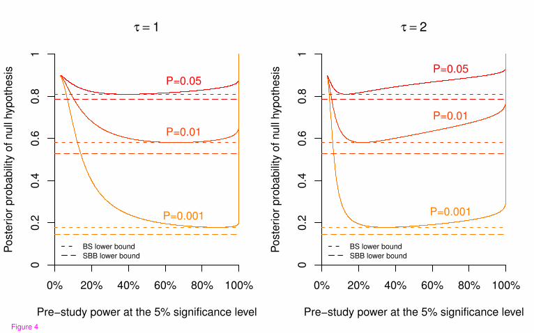
As emphasized in Spiegelhalter et al. [5, p. 130-133], the actual posterior probability of the null hypothesis

will also depend on the power (i.e. sample size) of the study. However, Hooper [15] has recently shown that

the evidence against the null hypothesis provided by a precise P value does not strongly depend on power

over the range of study sizes that are commonly encountered in clinical and epidemiological research. For

illustration, we reproduce in our Figure 4 the top panel of Figure 3 from Hooper [15], which gives the

posterior probability of the null hypothesis plotted against the (pre-study) power at the 5% significance

level for P = 0.05, 0.01, and 0.001. The calculation is based on a normal prior with mean µ0 and standard

deviation τ = 1 (left plot) and τ = 2 (right plot) under the alternative (assuming that one unit corresponds

to the minimum clinically important difference). This corresponds to Scenario 3 from Berger & Sellke [8].

We have added the corresponding BS lower bound (short dashed) on the posterior probability in Figure 4.

The actual posterior probability is quite close to this minimum for all powers typically encountered in

clinical research, say between 40% and 95%. This holds both for τ = 1 (left plot in Figure 4) and τ = 2

(right plot). Only for very small or very large studies the posterior probability is considerably greater than

the BS lower bound. The SBB bound, given by the long dashed line, is more conservative and hence

slightly lower than the BS lower bound.

In this paper I have adopted a Bayesian approach to calculate a lower bound on the posterior probability of

the null hypothesis, derived from a prior probability and a precise P value. Even Cox [16, p. 83] agrees

that “conclusions expressed in terms of probability are on the face of it more powerful than those expressed

indirectly via confidence intervals and P values. Further, in principle at least, they allow the inclusion of a

richer pool of [prior] information.” However, Cox feels that “conclusions derived from the frequentist

approach are more immediately secure than those derived from most Bayesian analysis” because [prior]

“information is typically more fragile or even nebulous as compared with that typically derived more

directly from the data under analysis”. On the other hand, Goodman [1,3, 6, 9] argues that the

misunderstanding and misuse of P values is so widespread that new tools are needed to properly convey

7

the strength of evidence provided by research data. The nomogram proposed in this paper is such a tool

and is particularly useful to study sensitivity to the prior probability of the null hypothesis, as illustrated

in Figure 2. Combined with a precise P value we obtain a range of plausible values for the posterior

probability of the null hypothesis, which is far easier to interpret than the P value itself.

Conclusions

The graphical device proposed in this paper enhances the understanding and facilitates the interpretation

of P values as measures of evidence against the null hypothesis among non-specialists. For study sizes

typically encountered in clinical and epidemiological research, the posterior probability of the null

hypothesis will be quite close to the lower bound provided by the nomogram. We are currently preparing a

JAVA applet at www.biostat.uzh.ch/static/pnomogram which allows to interactively use the proposed

nomogram on the internet.

Statement of competing interests

I declare that I have no competing interests.

Acknowledgements

I am grateful to Kaspar Rufibach and two referees for helpful comments on earlier versions of this

manuscript.

References1. Goodman SN: P Value. In Encyclopedia of Biostatistics, 2nd edition, Chichester: Wiley 2005:3921–3925.

2. Cohan J: The Earth is Round (p < .05). Am Psychol 1994, 49:997–1003.

3. Goodman SN: Towards Evidence-Based Medical Statistics. 1: The P Value Fallacy. Ann Int Med1999, 130:995–1004.

4. Hubbard R, Bayarri MJ: Confusion over measures of evidence (p’s) versus errors (α’s) in classicalstatistical testing (with discussion). Am Stat 2003, 57:171–182.

5. Spiegelhalter DJ, Abrams KR, Myles JP: Bayesian Approaches to Clinical Trials and Health-Care Evaluation.New York: Wiley 2004.

6. Goodman SN: Introduction to Bayesian methods I: measuring the strength of evidence. Clin Trials2005, 2:282–290.

7. Edwards W, Lindman H, Savage LJ: Bayesian Statistical Inference in Psychological Research. PsychRev 1963, 70:193–242.

8. Berger JO, Sellke T: Testing a point null hypothesis: Irreconcilability of P values and evidence(with discussion). J Am Stat Assoc 1987, 82:112–139.

9. Goodman SN: Towards Evidence-Based Medical Statistics. 2: The Bayes Factor. Ann Int Med 1999,130:1005–1013.

8

10. Sellke T, Bayarri MJ, Berger JO: Calibration of p Values for Testing Precise Null Hypotheses. Am Stat2001, 55:62–71.

11. Johnson VE: Bayes factors based on test statistics. J Roy Stat Soc B 2005, 67:689–701.

12. Deeks JJ, Altman DG: Diagnostic tests 4: likelihood ratios. Brit Med J 2004, 329:168–169.

13. Fagan TJ: Letter: Nomogram for Bayes theorem. N Engl J Med 1975, 293:257.

14. Spiegelhalter DJ, Myles JP, Jones DR, Abrams KR: Bayesian Methods in Health TechnologyAssessment: A Review. Health Technol Assess 2000, 4(38).

15. Hooper R: The Bayesian interpretation of a P -value depends only weakly on statistical power inrealistic situations. J Clin Epidemiol 2009, 62:1242–1247.

16. Cox DR: Principles of Statistical Inference. Cambridge: Cambridge University Press 2005.

FiguresFigure 1 - A nomogram for P values.

The prior probability for the null hypothesis is located on the first axis, the observed P value on the second

axis, and the minimum posterior probability on the third axis.

Figure 2 - Application to lung cancer CHART trial.

For a P value of 0.3% (0.003), the lower bound on the posterior probability can be read off the third axis

for a q = 10% (green line), q = 50% (red line), and q = 90% (blue line) prior probability.

Figure 3 - Application to lung cancer CHART trial.

The prior probability must be 6% or smaller to obtain a lower bound of 0.3% on the posterior probability

(red line). The green line indicates, that we need a P value of 0.014% (0.00014) or smaller to reduce the

probability of the null hypothesis from q = 50% a priori to 0.3% a posteriori.

Figure 4 - Dependence of the posterior probability on study power.

Posterior probability of the null hypothesis plotted against the (pre-study) power at the 5% significance

level for P = 0.05, 0.01, and 0.001 and a prior probability of q = 90%. The calculation is based on a normal

prior with standard deviation τ = 1 (left plot) and τ = 2 (right plot) under the alternative, assuming that

one unit corresponds to the minimum clinically important difference. The dashed lines indicate the

minimum posterior probability as obtained from the BS (short dashed) and SBB (long dashed) approach,

respectively.

9

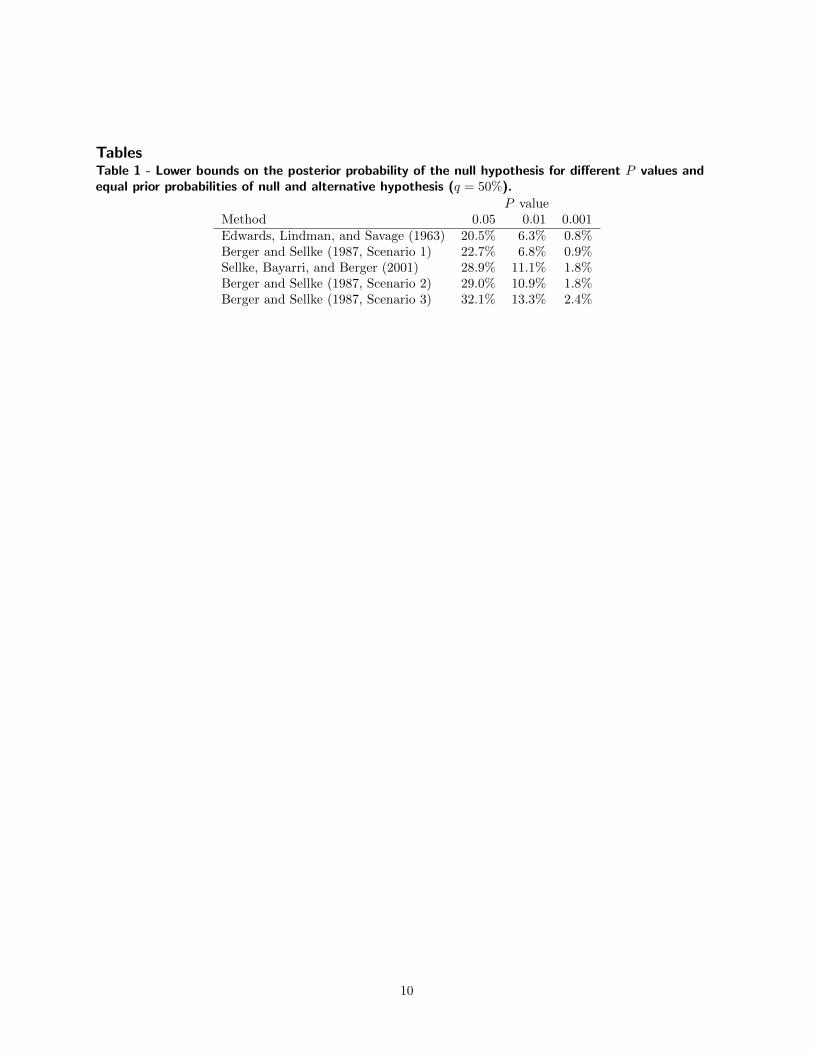
TablesTable 1 - Lower bounds on the posterior probability of the null hypothesis for different P values andequal prior probabilities of null and alternative hypothesis (q = 50%).

P valueMethod 0.05 0.01 0.001Edwards, Lindman, and Savage (1963) 20.5% 6.3% 0.8%Berger and Sellke (1987, Scenario 1) 22.7% 6.8% 0.9%Sellke, Bayarri, and Berger (2001) 28.9% 11.1% 1.8%Berger and Sellke (1987, Scenario 2) 29.0% 10.9% 1.8%Berger and Sellke (1987, Scenario 3) 32.1% 13.3% 2.4%

10

0.5

1

2

5

10

20

30

40

505050

60

70

80

90

95

98

99

99.5

1e−06

1e−05

1e−04

0.001

0.01

0.05

0.37

0.001

0.002

0.005

0.01

0.02

0.05

0.1

0.2

0.5

1

2

5

10

15

20

30

40

5050

% %

Prior P value Min. Posterior

Probability Probability

Figure 1

0.5

1

2

5

10

20

30

40

505050

60

70

80

90

95

98

99

99.5

1e−06

1e−05

1e−04

0.001

0.01

0.05

0.37

0.001

0.002

0.005

0.01

0.02

0.05

0.1

0.2

0.5

1

2

5

10

15

20

30

40

5050

% %

Prior P value Min. Posterior

Probability Probability

Figure 2

0.5

1

2

5

10

20

30

40

505050

60

70

80

90

95

98

99

99.5

1e−06

1e−05

1e−04

0.001

0.01

0.05

0.37

0.001

0.002

0.005

0.01

0.02

0.05

0.1

0.2

0.5

1

2

5

10

15

20

30

40

5050

% %

Prior P value Min. Posterior

Probability Probability

Figure 3

Pre−study power at the 5% significance level

Poste

rior

pro

babili

ty o

f null

hypoth

esis

0% 20% 40% 60% 80% 100%

00.2

0.4

0.6

0.8

1

P=0.05

P=0.01

P=0.001

τ = 1

BS lower bound

SBB lower bound

Pre−study power at the 5% significance level

Poste

rior

pro

babili

ty o

f null

hypoth

esis

0% 20% 40% 60% 80% 100%

00.2

0.4

0.6

0.8

1

P=0.05

P=0.01

P=0.001

τ = 2

BS lower bound

SBB lower bound

Figure 4