This Provisional PDF corresponds to the article as it appeared upon acceptance. Fully formattedPDF and full text (HTML) versions will be made available soon.

Statistical Analysis of Dendritic Spine Distributions in Rat Hippocampal Cultures

BMC Bioinformatics 2013, 14:287 doi:10.1186/1471-2105-14-287

Aruna Jammalamadaka (arunaj@ece.ucsb.edu)Sourav Banerjee (sourav.banerjee@lifesci.ucsb.edu)Kenneth S Kosik (kenneth.kosik@lifesci.ucsb.edu)

Bangalore S Manjunath (manj@ece.ucsb.edu)

ISSN 1471-2105

Article type Research article

Submission date 7 February 2013

Acceptance date 16 September 2013

Publication date 2 October 2013

Article URL http://www.biomedcentral.com/1471-2105/14/287

Like all articles in BMC journals, this peer-reviewed article can be downloaded, printed anddistributed freely for any purposes (see copyright notice below).

Articles in BMC journals are listed in PubMed and archived at PubMed Central.

For information about publishing your research in BMC journals or any BioMed Central journal, go to

http://www.biomedcentral.com/info/authors/

BMC Bioinformatics

© 2013 Jammalamadaka et al.This is an open access article distributed under the terms of the Creative Commons Attribution License (http://creativecommons.org/licenses/by/2.0), which

permits unrestricted use, distribution, and reproduction in any medium, provided the original work is properly cited.

Statistical analysis of dendritic spine distributionsin rat hippocampal cultures

Aruna Jammalamadaka1∗

∗Corresponding authorEmail: arunaj@ece.ucsb.edu

Sourav Banerjee2

Email: sourav.banerjee@lifesci.ucsb.edu

Bangalore S Manjunath1

Email: manj@ece.ucsb.edu

Kenneth S Kosik2∗∗Corresponding authorEmail: kenneth.kosik@lifesci.ucsb.edu

1Department of Electrical and Computer Engineering, University of CaliforniaSanta Barbara, Santa Barbara, CA, USA

2Department of Molecular and Cellular Neurobiology, University of CaliforniaSanta Barbara, Santa Barbara, CA, USA

Abstract

Background

Dendritic spines serve as key computational structures in brain plasticity. Much remains to be learnedabout their spatial and temporal distribution among neurons. Our aim in this study was to performexploratory analyses based on the population distributions of dendritic spines with regard to theirmorphological characteristics and period of growth in dissociated hippocampal neurons. We fit a log-linear model to the contingency table of spine features suchas spine type and distance from the somato first determine which features were important in modelingthe spines, as well as the relationshipsbetween such features. A multinomial logistic regression was then used to predict the spine typesusing the features suggested by the log-linear model, alongwith neighboring spine information.Finally, an important variant of Ripley’s K-function applicable to linear networks was used to studythe spatial distribution of spines along dendrites.

Results

Our study indicated that in the culture system, (i) dendritic spine densities were “completelyspatially random", (ii) spine type and distance from the soma were independent quantities, and mostimportantly, (iii) spines had a tendency to cluster with other spines of the same type.

Conclusions

Although these results may vary with other systems, our primary contribution is the set of statisticaltools for morphological modeling of spines which can be usedto assess neuronal cultures followinggene manipulation such as RNAi, and to study induced pluripotent stem cells differentiated toneurons.

Keywords

Dendritic spines, Rat hippocampal culture, Linear networkK-function, Morphological modeling,Spatial statistics, Point processes, Neuronal growth

Background

Spines are protrusions that occur on the dendrites of most mammalian neurons. They contain the post-synaptic apparatus and have a role in learning and memory storage. Spine distribution is a criticallyimportant question for multiple reasons. Changes in spine distributions and shape have been linked toneurological disorders such as Fragile X syndrome [1]. Spine distributions determine the extent to whichthe neuropil will be electrically sampled, i.e. dense distributions will sample the neural connectivitymap more fully [2]. Furthermore, the nature of optimal sampling is unknown and likely depends onthe surrounding anatomy and the total information content available to dendrites. Because pruning takesplace during development in an activity dependent manner, spine distributions may reflect activity withinneural circuits. Distributions of spine types are biologically important because the electrical propertiesof spines, such as the spine neck resistance, promote nonlinear dendritic processing and associated formsof plasticity and storage [3] to enhance the computational capabilities of neurons.

The shapes and types of dendritic spines contribute to synaptic plasticity. Because neighboring spineson the same short segment of dendrite can express a full rangeof structural dimensions, individualspines might act as separate computational units [4]. Nevertheless, the dendrite acts in a coordinatedmanner and thus the spatio-temporal distributions of different spine types is likely to be significant.Little is known about this population level organization ofdendritic spines. Our aim was to perform anexploratory analysis of neuronal data from different time periods during the growth of rat dissociatedhippocampal neurons, a well-established model system [5].The observations here pertain only to theculture system and not necessarily to in vivo settings although the analytical tools used here could beadapted to in vivo analyses.

By quantifying populations of dendritic spines with automated tools at a global level, we were ableto perform a much larger and more comprehensive analysis than most previous studies. Many studiesonly analyze a small region of interest on the largest dendrites, for example the 50–75µm closest tothe soma [6], or10 µm segments [7], making it easier to measure manually the spinetype counts anddimensions. Other works determine spine lengths and widthsby manually drawing a line along themaximal length and measuring the length of that line [8], andtherefore are only able to analyze a fewneurons and a few hundred spines at a time.

In this study we determined the ratios of spine types along the dendrites as a function of time in culture,clustering or repulsion of spines in space, and how best to model spine type distributions. A model thatfits the spatial distribution of spine types in healthy cultured neurons would be useful to assess neuronalcultures following gene manipulation such as RNAi and to study features of induced pluripotent stemcells differentiated to neurons.

Log-Linear Models (LLM) and Multinomial Logistic Regressions (MLR) are two basic and essentialstatistical methods, and have an extensive history of beingused in biological studies. However, thesetools have not been used thus far in the analysis of spine distributions. We fit a log-linear model (LLM)to the contingency table of spine features to determine the dependence between spine types (mushroom,thin, and stubby), distance from the cell body along the dendrite (in micrometers), the branch order of thedendritic segment on which it lies (primary, secondary, tertiary, etc.), and the day in vitro (DIV) on whichit was imaged. Once we determined which of these attributes contributed to the overall dendritic spinemodel, we then asked whether these attributes can predict the occurrence of spines and of spine types.

To answer this question we used a Multinomial Logistic Regression (MLR) model, which predictedthe spine type, using the attributes that were found to be important through the LLM and associatedcontingency tables.

Finally, to understand how the dendritic spine density varied over the length of the neuron or whetherthe appearance of spines was completely spatially random i.e uniformly distributed over the neurites, wemade use of spatial point processes. Spatial point processes have been used before in biological studiesto model the locations of entire neurons [9-11], locations of ants nests [12] or xylem conduits [13].There have also been other more ad-hoc methods created to study the number of “clustered spines” oneach dendritic segment in monkey brains, where a cluster is defined as a group of 3 or more spines [14]however we believe our use of the linear network K-function [15] is the first work to analyze the locationsof dendritic spines and their clustering properties in sucha principled manner. Our analysis indicatedthat the density of spines is generally completely spatially random (CSR) over the dendritic lengthprobably due to the absence of instructive directional signals found an in vivo setting in which spinedistributions are unlikely to be CSR.

Methods

Cell imaging

Dissociated hippocampal neurons from embryonic rat brains(E18) were plated onto poly-l-lysine coatedcoverslips. Once neurons adhered to the coverslip, they were placed face-down on glial cells grown invitro for 15 days. These neurons were a primary neuronal culture system, and no cell line was used.Neurons were grown for specific time periods up to 21 days in a neuronal medium containing B27. Thisco-culture of neurons and glia mimic the physiological conditions of neuronal growth and developmentin mammalian brain [5]. Work with the neuronal cultures was approved by the UCSB animal carecommittee.

To fill the neuronal processes including dendritic spines Green Fluorescent Protein (GFP) wasexpressed from a plasmid containing the beta-actin promoter (CAG-GFP) [16]. Of this plasmid,2 µgwas transfected into each coverslip containing about50, 000 neurons (including about20% glial cells).Transfection was performed as described in the manufacturer’s protocol (Lipofectamine 2000 fromInvitrogen) with minor changes. The transfection mix and neurons were incubated for two hours toavoid toxicity caused by lipo2000. Following transfection, coverslips were flipped back onto the glialdish, where they were originally cultured. GFP-actin transfected into the neurons at DIV4 (Day InVitro) and neurons were studied at three time points- DIV7, 14 and 21. These time points survey thematuration period over which synapses and spines emerge [17]. Note that these were not the sameneurons studied over time, but each time point represents a different population of neurons which weregrown in culture up until the point of imaging. In this way ouranalysis represents a study at thepopulation level. At each time point the number of images taken per plate depended on the transfectionefficiency of that plate. On average approximately1% of cells were transfected. The plating densitywas set so that neurons were relatively isolated in order to capture one neuron per image. An OlympusFluoView laser scanning confocal microscope was used. Image slices were2048 by 2048 pixels at154nm per pixel resolution. There were7–33 z-slices per stack depending on the depth of the neuron,taken at200nm steps. This means that the stacks were315.39 µm× 315.39 µm× 1.4–6.6 µm. The zdimension slices were used to capture each depth level at theoptimal focus, however we cannot claimto have accurate volumetric information at this resolution. A 40X oil objective lens with no opticalzoom was used. Numerical Aperture (NA) was1.3, and illumination conditions were kept constant.Deconvolution of the raw data before processing was not necessary because the images were clearenough to manually annotate the neuron traces and manually edit all the spine detections and types asdescribed in the following section. We performed three biological replicates, the results of which are

detailed below.

Although there are other higher resolution, full volume methods, the analysis of this data is broadlyapplicable to imaged neurons in other systems [5]. We attempted to capture the entire neuron in eachimage, however because of limits in available imaging techniques we found that this does not alwayshappen. In the cases where dendrites were truncated at the end of the image plane we assumed that theproportion of spines in the missing data was similar to what had already been observed, and thereforethe resulting distributions did not change. We verified thisassumption visually by taking tiled mosaicsof a few neurons imaged in their entirety from each DIV and checking that the branch orders, distancesto soma and spine type counts were unchanged as compared to those of the same DIV. There was anobserved increase in the dendritic length truncated by the image plane as the DIV increased. Howeverin our particular analyses the methods used, such as the Log-Linear Model and Multinomial LogisticRegression, were focused on trends between spine characteristics such as distance to soma and typeand these trends are innately unaffected by the truncation of dendrites given the above assumption.In addition, spatial point process analyses such as the linear network K-function always include thespecification of an observation window [18], which in our case was the image plane. We verified (seeResults and discussion section) that the overall spine density and the density of each spine type did notvary with distance from the soma so that we could assume spinedensity at the ends of the dendriteswhich were truncated was similar to the dendritic length which was observed. We recognize that wecannot see the proximity of labeled cells to other neurons which haven’t taken up the GFP labeling.These unlabeled neighboring neurons may cause some difference in spine distributions which we cannotquantify. For this reason we have attempted to quantify our biological findings statistically over entireexperiments and DIV time points instead of by individual neurons, although in certain cases showingresults from individual randomly sampled neurons was necessary.

Neuronal reconstruction

There exist many automated methods for studying neuronal growth and morphometry and therefore wepresent a brief review of available software for tracing dendrites and detecting and classifying spines.In particular, NeuronJ [19] is a widely used software; however it is only semi- automatic and one mustclick several points to trace each neurite. The labeling is done manually and the statistics output onlyinclude lengths of neurites and not spine data. HCA-Vision [20] is a costly software with similar goals,however the parameters of the neurite tracing are set manually with a sliding bar and thus results requiremuch hand-tuning. In addition, it is also focused on tracingneurites as opposed to spine analysis. For afull review of existing methods and softwares for neuron tracing and spine detection see [21]. We foundNeuronStudio [22-24] to be the most user-friendly, and for this reason we used it to annotate dendritesand spines for this analysis.

Despite the abundance of automated softwares, neuronal reconstructions are still largely performed byhand [25] and this is is especially essential for a study likethis one, where the traversed distance ofthe dendrites and number of spines and their shapes were analyzed in such detail. Using automatedreconstruction algorithms on raw data is prone to both falsepositive and false negative detections ofspines, as well as misleading spine shape measurements. In cases where neurites from neighboringneurons enter into an image (e.g. Figure 1 panes B and C), NeuronStudio often incorrectly tracesthese neurites as belonging to the neuron of interest. For this reason we manually traced each dendriticbranch and soma of each neuron, ran NeuronStudio’s automated spine detection/classification algorithmand then manually inspected and verified each spine’s location and type. The verification and tracingwere done by the primary author and an undergraduate biologystudent working in the Kosik Lab (seeAcknowledgments). They were both familiar with dendrite and spine morphology and the resultingannotations from each were cross-checked by the other.

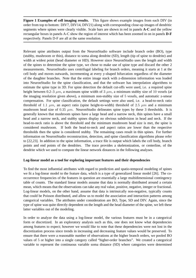
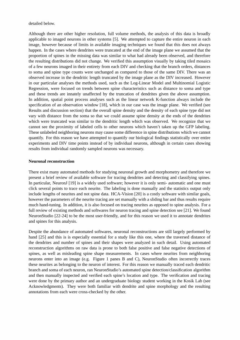
Figure 1 Examples of cell imaging results. This figure shows example images from each DIV (inorder from top to bottom: DIV7, DIV14, DIV21) along with corresponding close-up images of dendriticsegments where spines were clearly visible. Scale bars are shown in red in panelsA-C and the yellowrectangular boxes in panels A-C show the region of interest which has been zoomed in on in panelsD-Frespectively. Panels D-F are all at the same resolution.

Relevant spine attributes output from the NeuronStudio software include branch order (BO), type(stubby, mushroom or thin), distance to soma along dendrite(SD), length (tip of spine to dendrite) andwidth at widest point (head diameter or HD). However since NeuronStudio uses the length and widthof the spines to determine the spine type, we chose to make useof spine type and discard the other 2measurements. NeuronStudio uses centrifugal labeling forbranch orders, meaning it starts at 1 at thecell body and moves outwards, incrementing at every y-shaped bifurcation regardless of the diameterof the daughter branches. Note that the entire image stack with z-dimension information was loadedinto NeuronStudio for the spine classification, and that thesoftware has interpolation algorithms toestimate the spine type in 3D. For spine detection the default cut-offs were used, i.e. a required spineheight between 0.2–3µm, a maximum spine width of3 µm, a minimum stubby size of10 voxels (atthe imaging resolution given above), a minimum non-stubby size of 5 voxels, and automatic z-smearcompensation. For spine classification, the default settings were also used, i.e. a head-to-neck ratiothreshold of1.1 µm, an aspect ratio (spine height-to-width) threshold of2.5 µm and a minimummushroom head size of0.35 µm. NeuronStudio delineates spine types by these 3 thresholds. It isgenerally known that mushroom spines have a large head and a narrow neck, thin spines have a smallhead and a narrow neck, and stubby spines display no obvious subdivision in head and neck. If thehead-to-neck ratio is above the threshold and the minimum mushroom head size is met, the spine isconsidered mushroom. If both the head-to-neck and aspect ratios are lower than the respectivethresholds then the spine is considered stubby. The remaining cases result in thin spines. For furtherinformation on NeuronStudio reconstruction, detection, and spine classification algorithms please referto [22,23]. In addition to the spine information, a trace fileis output which labels the cell body, branchpoints and end points of the dendrites. The trace provides a skeletonization, or centerline, of thedendrite which we used to compute the linear network distances in the following analyses.

Log-linear model as a tool for exploring important featuresand their dependencies

To find the most influential attributes with regard to prediction and spatio-temporal modeling of spineswe fit a log-linear model to the feature data, which is a type ofgeneralized linear model [26]. The co-occurrence frequencies of the features in question are essentially a large multidimensional contingencytable of counts. The standard linear models assume that datais normally distributed around a certainmean, which means that the observations can take any real value, positive, negative, integer or fractional.Log-linear models, on the other hand, assume that data is intrinsically non-negative, typically countsthat could be Poisson distributed, and allow us to model the association and interaction patterns amongcategorical variables. The attributes under consideration are BO, Type, SD and DIV. Again, since thetype of spine was quite directly dependent on the length and the head diameter of the spine, we left theselatter variables out of the modeling.

In order to analyze the data using a log-linear model, the various features must be in a categoricalform or discretized. In an exploratory analysis such as this, one does not know what dependenciesamong features to expect; however we would like to note that these dependencies were not lost in thediscretization process since trends in increasing and decreasing feature values would be preserved. Toensure that there were a reasonable number of observations at the higher branch orders, we pooled BOvalues of5 or higher into a single category called “higher-order branches”. We created a categoricalvariable to represent the continuous variable soma distance (SD) where categories were determined

using the4 quartiles of the SD spine data pooled over all3 experiments. Specifically, SD values of lessthan65.65 µm were classified into the first group, from this value to less than108.99 µm the second,from this to less than157.04 µm the third, and the rest (less than the most distal spine whichlay at413.25 µm from the cell body) fell in the fourth group. Binning the observed data for the continuousvariables is the best way to get a general feel for how these quantities relate to each other. After thispost-processing of the data we arrived at5 categories of branch order,4 categories of soma distance,3spine types (mushroom, stubby, and thin), and3 DIVs (7, 14, and 21 days).

Using the observed frequencies for the aforementioned attributes, we created a four-way contingencytable and fit the model using the ‘glm’ function in the R package ‘stats’. The table of the frequency ofoccurrences of the four attributes was modeled as Poisson with each entry being a simple count of theco-occurrences of that bin. We called this countfijkl with each of the subscriptsi, j, k, l correspondingto a different attribute. The method uses the link functionyijkl = log(fijkl), and treats the model as aregular linear model. Each entryyijkl is modeled by a combination of coefficients: the intercept, plusmain effects, plus every combination of interactions between these four attributes, as shown below.

yijkl = µ+ αi + βj + γk + δl + (αβ)ij + (αγ)ik + (αδ)il + . . .+ error. (1)

We estimated this full interaction model using the least-squares maximum-likelihood approach. We alsoused a stepwise fit algorithm, which begins with a model that includes only the constant term, and ateach step chooses whether or not to add one additional term. The algorithm begins with the main effectsthen tries each possible 2-way interaction, aiming to minimize the Akaike Information Criterion (AIC).The AIC is defined as

AIC = 2k − 2ln(L(θ|y,x)) (2)

wherek is the number of parameters i.e the total number of coefficients being estimated, and

L(θ|y,x) = maxθ

N∏

n=1

eynθ′xne−eθ

′xn

yn!(3)

is the maximized value of the likelihood function for the estimated Poisson model. In the aboveequationsx = x1, . . . , xN ∈ R

4 are the input vectors,θ = θ1 . . . θk are the parameter values (one perterm in eqn. 1), andy = y1, . . . , yN ∈ R is the output. The AIC is a commonly used goodness-of-fitmeasure for a model given the observed data. Adding or subtracting terms, whether they be maineffects, pairwise interactions, or up to 3-way interactions between attributes, will change the AIC valuefor the model. A lower AIC criterion indicates a better fit to the data and therefore a better model. Tocompute the stepwise fit we used the R function ‘step’. For more information on the stepwise fitalgorithm as well as the AIC criterion we ask that the readersrefer to the ‘step’ function reference( [27], Chapter 6). We ran both of these LLM fitting proceduresfor all 3 experiments separatelyexpecting to find general agreement between coefficients of the corresponding models created.

Multinomial logistic regression to predict spine type from neighbor types

In order to predict spine type we first determined which attributes contributed most to spine typeprediction. Given the complexity of the multidimensional LLM and the various interactions andconditional frequencies that would impinge on this issue, we decided to determine these attributes byanalyzing 2-way contingency tables for spine type vs. SD, BO, DIV, as well as the spine types of the 3nearest neighbors. This analysis helped us pick attributesthat would be useful as the predictors in themultinomial logistic regression (MLR) [28] explained below.

When the response variable of a regression takes binary values “Logistic Regression” is used. Thisis an approach which uses a linear combination of the predictor variables to predict the log-odds of

a success (the “logit” of the probability). Since our response variable was spine type and it can take 3values (mushroom, stubby or thin), we needed to use a “Multinomial Logistic Regression” (MLR) whichattempts to model the probability of any of multiple possible outcomes. We did not use the attributesSD or BO as predictors variables since the results of both theLLM analysis and 2-way contingencytables mentioned above told us that these quantities were not as relevant for spine type prediction.Therefore our model consisted of spine type as the output variable and the DIV, 1st, 2nd and 3rd nearestneighbor type along the dendrite as the predictor variables. We tried using only 1 or 2 nearest neighbors,however the results proved inconclusive because the prediction probabilities for each of the 3 typeswere predominantly close to1/3. If we used more than the 3 nearest neighbors we sometimes ended upspanning a segment of dendrite which we did not consider to be“local”, so we decided that 3 nearestneighbors provide the most useful information in the case ofthis study.

The MLR analysis we performed in this paper does disregard the actual inter-spine distances, meaningthat if the 3 nearest neighbors are very close or very far apart we still treat them the same. We didthis partially because adding the distance variables wouldcomplicate the model significantly, but alsobecause we believe that over a large population of spines such as the one we have, these differences indistance will average out and we will still get a general picture of the trends between neighboring spinetypes. To verify that this was true we computed a histogram showing the distribution of 3rd nearestneighbor distances for each spine, shown in Figure 2. Although the maximum distance to any 3rdnearest neighbor is extremely high (248.31 µm) we can see from the histogram as well as the fact thatthe median 3rd nearest neighbor distance was5.34 µm that this distance is clearly an outlier case andthat the majority of 3rd nearest neighbor distances lie below 25 µm.

Figure 2 Histogram of 3rd nearest neighbor distances. This figure shows the distribution of 3rdnearest neighbor distances in order to get an idea of the physical neighborhood of spine types used forthe MLR. It shows that although the maximum distance to any 3rd nearest neighbor was extremely high(248.31 µm) this distance was clearly an outlier case.

Suppose the output variable categories are denoted by0, 1, 2 corresponding to mushroom, stubby orthin spines, with0 being the reference category. Ifyi denotes the observed outcome of the outputvariable (spine type), andXi is the corresponding vector of the 3 neighbor types and DIV for the ithobservation, one regression is run for the logit probability of each categoryk, with βk representing thevector of regression coefficients in thekth regression (eqns. 4,5). This is done for all but the referencecategory, whose probability is then obtained by subtracting all other probabilities from one (eqn. 6).Note that because the predictor variables were spine types,which were nominal as opposed to ordinalvariables, the predictor variablesXi must be represented with a “dummy coding”. This means eachneighbor type was represented by 2 predictor variables, where (1, 0) corresponded to mushroom type,(0, 1) corresponded to stubby type and(0, 0) corresponded to thin type. This does not need to be donefor the output variabley. With the addition of the DIV, which does not have to be dummy coded since itis an ordinal variable, this made eachXi vector of length 7.

The regressions are then written as:

P (yi = 1) =exp(β1Xi)

1 + exp(β1Xi) + exp(β2Xi)(4)

P (yi = 2) =exp(β2Xi)

1 + exp(β1Xi) + exp(β2Xi)(5)

and

P (yi = 0) = 1− P (yi = 1)− P (yi = 2) =1

1 + exp(β1Xi) + exp(β2Xi)(6)

The parameters are estimated typically by using an iterative procedure such as “iteratively re-weightedleast squares” (IRLS) or, more commonly by a numerical approach (a quasi-Newton method) such as theBroyden-Fletcher-Goldfarb-Shanno (BFGS) method. In our case we create an MLR using the commandmultinomin the R package nnet [29] which uses BFGS by calling the R function optim. It can be seenthat

log(P (yi = 1)

P (yi = 0)) = β1Xi (7)

log(P (yi = 2)

P (yi = 0)) = β2Xi (8)

so that the beta coefficients represent the change in the log odds of the dependent variable being in aparticular category with respect to the reference categoryi.e. the thin type, for a unit change of thecorresponding independent variable. To check if the modelscreated from all three experiments were inagreement, we ran the MLR separately for each experiment.

To satisfy one of the major assumptions of this analysis, namely that the data must be a set of independentobservations, we took200 randomly sampled spines of each type from each experiment (600 spines perexperiment total) to use for the parameter estimation. We chose to select equal proportions of each spinetype in order to remove any bias in the model towards the less frequent thin spines, and200 was thelargest number we could justify using since there were only649 thin spines in experiment3. We verifiedthat these randomly sampled spines did not lie within10 µm of the image border so that we were fairlycertain their nearest neighbors did not fall outside of the image plane. Note that due to the tortuosity ofthe dendritic structure this did not mean that our sample wasnecessarily biased towards spines whichwere proximal to the soma. We did not verify explicitly that the sampled spines were not neighborsof each other, since we assumed that the variation captured by the random sampling was enough toensure some level of independence. The idea was to aim for an independent set of observations whichrepresented the entire “population” of spines in that experiment.To be clear we used all30, 285 spinesfor the LLM model and K-function analysis, only the MLR modelrequired random sampling since wewere using neighbor information which would have been redundant if we considered every spine.

To verify that the prediction of spine type provided by the MLR was better than what we would get purelyby their relative abundance i.e. without neighboring spinetype information, we computed somethingsimilar to a “Bayes Factor” [30]. Bayes factor is a method of choosing between two models on thebasis of the observed data. In our case, the first prediction model was simply the prior global probabilityof finding a given spine type based on its frequency in the particular experiment under consideration.The second model was the MLR prediction model using the neighbor type information. We computedP (Y = i|X)/P (Y = i) and reasoned that values considerably larger than one indicated the neighboringspine type information was helpful in the prediction of the central spine type.

Linear network K-function as a tool for testing spatial point patterns

Originally proposed by Ripley in 1981 [31], the purpose of the K-function is to estimate whether or notthere is clustering or repulsion present in a given spatial point process. The common null hypothesis isthat the points within the observation window are distributed as a homogeneous Poisson process, whichis also termed “completely spatially random” or CSR. This means that the density of points does notvary depending on the spatial parameters i.e. x and y in the 2DEuclidean case, or the location alongthe dendritic network in our case. In order to determine if this is a valid null hypothesis for our data,we created Q-Q plots [32] for individual dendrites which compared the quantiles of the SD values ofobserved spines to the theoretical quantiles for the CSR case. If the two distributions (observed and CSR)being compared were similar, the points in the Q-Q plot wouldapproximately lie on the liney = x. Inorder to create the theoretical quantiles it is necessary toknow the values of SD at any location on thegiven network, not just at the spine locations. Once we have this we can partition the network into

epsilon small segments and assign each segment a value1 if it contains a spine and0 otherwise basedon the CSR assumptions. We did this using code provided to us by Adrian Baddeley and Gopal Nair atthe Commonwealth Scientific and Industrial Research Organization (CSIRO), Australia.

The K-function computes the expected number of points within a distancet of an arbitrary pointp,therefore the empirical value in 2D Euclidean space for the CSR case will be proportional to the circulararea,λπt2. The proportionality constantλ represents the density of points in the homogeneous Poissoncase, and can be estimated by finding the total number of points N divided by the total area of theobservation windowA. Ripley’s K-function, which is a function oft, is a very useful tool because itdescribes the2nd order characteristics of the point process at several scales t. If we ignore the edgeeffects due to the observation window, the observedK̂(t) can be written as:

K̂(t) =|A|

N2

∑

i

∑

j 6=i

I(dij < t) (9)

whereI stands for the indicator function, anddij stands for the Euclidean distance between two pointspi andpj. In the above equation, we see that the expectation is normalized by1/λ sinceλ = N

|A| , so

we infer that theoreticallyK(t) = πt2 implies spatial independence of points, or a CSR point process.Therefore, ifK(t) is the theoretical CSR value of the function andK̂(t) is the observed function, thenK̂(t) > K(t) implies clustering between points and̂K(t) < K(t) implies repulsion. It is possible toextend this function to multi-type point patterns (i.e. to find clustering or repulsion between specificspine types) or to higher dimensional data (i.e. space-time, or 3D Euclidean space).

Since our particular point process consists of spines whichlie along the “linear network” of thedendritic tree we were primarily concerned with inter-spine distances along the dendrite as opposed toin Euclidean space. Therefore we used a version of the K-function developed recently for linearnetworks by Okabe and Yamada [15]. This modified version of the K-function takes into account thestructure of the linear network on which the point process resides and imitates the Euclidean spaceK-function described above. The linear network K-functionis calculated as follows:

K̂(t) =`TN2

N∑

i=1

∑

j 6=i

I(dij < t) (10)

where`T is the length of the total networkLT . The theoretical CSR for this case is described as follows:

K(t) =1

`T

∫

p∈LT

`p(t)dp (11)

wherep is a point belonging to the set of all pointsP = {p1, ..., pN}, and`p(t) is the length of thesubset of the networkLp(t) where the distance between p and any other point is≤ t. Note that herethe distancedij stands for the linear network distance along the dendrite. Accounting for variability inthe length`p(t) means the formula takes into account the edge effects due to the observation window(in our case the image plane) inherently, but at the cost of added complexity. The computation of thetheoretical linear network K-function requires us to findLpi(t), the subset ofLT where the networkdistance between a specific pointpi and any other point is≤ t, and`pi(t), the length of that subset, forevery pointpi. A visualization of the quantitiesdij , LT , `T , Lpi(t), and`pi(t) is shown in Figure 3.

Note that although many biological applications of point processes treat individual observations asreplicate patterns coming from the same underlying distribution, we cannot do that using the abovedefinition of the network linear K-function due to the changein linear network structure from dendriteto dendrite. The term “dendrite” here refers to the entire dendritic tree resulting from a single rootbranch of a neuron. Other in-vivo studies [33,34] focus on clustering of spines which lie on the sameunbranched section of the dendrite, however we focus on the entire dendritic tree under the hypothesis

Figure 3 Visualization of the linear network K-function. This figure clarifies what is meant by thequantitiesdij , LT , `T , Lpi(t), and`pi(t) which were used to compute the linear network K-function.Heredij is the linear network distance shown by the gray line betweenpointspi andpj. LT (in black) isthe entirety of the single dendritic network and`T is the length ofLT . Similarly,Lpi(t) (in blue dashedlines) is subset of the network where the distance between a point pi and any other point is≤ t and`pi(t) is the length ofLpi(t). In this particular example there are2 spines which fall withinLpi(t) andwould be counted in determining the empirical function value K̂(t), however pointpj falls outside thisradius and would therefore not be counted.

that it follows rule-based distributions of spines due to anatomical constraints and integration of the asignal over the entire dendrite. One can infer from Figure 3 that since the geometry of the linearnetwork changes from dendrite to dendrite, so do the total lengths of the networks̀T , the ranges ofpossible t-values and the amount of dendritic length that ispresent within a given distance of any point.We did not simply normalize the lengths of the networks to a[0, 1] scale because it is desirable for thet-axis to retain its real physical values in order to make conclusions about the scale (inµm) ofclustering or repulsion among spines. However, we did desire to compare the linear networkK-functions of various dendrites in a meaningful way. For this reason we used a corrected version ofthe network K-function that intrinsically compensates forthe geometry of the network called Ang’scorrection [35]. The observed K-function then becomes:

K̂(t) =`T

N(N − 1)

N∑

i=1

∑

j 6=i

I(dij ≤ t)

m(i, dij)(12)

wherem(i, dij) is the number of points ofL lying at the exact distancet away from the pointi measuredby the shortest path. That is, the contribution to the function from each pair of points(i, j) is weightedby the reciprocal of the number of points that are situated atthe same distance fromi asj is. As a result,the theoretical CSR case is simplyK(t) = t for all 0 ≤ t < T . This enables direct comparison oft-values across dendrites, as we will see in the results section.

Simulations and q-values

To test the null hypothesis that the locations of spines on the dendrites were indeed CSR, we createda summary statistic which encompasses the difference between the empiricalK̂(t) and the theoreticalK(t) under CSR. The summary or “test statistic” we used, is the maxabsolute difference (MAD) overt, viz.

d = maxt

|K(t)− K̂(t)|.

One method for obtaining a distribution ofd proposed by Diggle [36] is to bootstrap the residuals, ordifferences between the observed and theoretical values. However a more heuristic and intuitive way isto simulate the CSR case for each dendrite, compute the K-function for each of these simulations, andfind the simulated distribution of our test statistic. We then found the p-value of the observed differenced from this simulated distribution.

Specifically, we carried out1000 CSR simulations for each dendrite by placing uniform pointson a line[0, `T ], and mapping them to that specific dendrite’s linear networkstructure. The number of pointssimulated per dendrite equaled the number of observed spines for that dendrite, thus preserving theoverall densityλ. This means the same number of spines that existed on each dendrite were randomlyplaced along the linear network specific to that dendrite. Weused these simulations to obtain1000values of the summary statistic, sayd[i]. Then the p-value for each dendrite was simply the proportion

of simulated values that fell above the observed or experimental value ofd, i.e. the rank of thisd withinthe1000 values ofd[i], ornrank/(nsim+ 1).

This p-value approach is similar to the test which rejects the null hypothesis if the graph of the observedK-function lies outside the “point-wise simulation envelope” at any value of t. A simulation envelopeis essentially a graphical measure of how far a function can deviate from the theoretical value withoutbeing considered significant at a given level. As mentioned above in our case the envelope is calculatedby first creating the1000 CSR simulations of a point pattern on a given dendritic network with the sameobserved network intensity, then calculating the linear K-function for each of these1000 simulations. Toperform a two-sided significance test at the10% level, the5% and95% percentiles are then calculatedbased off the50 lowest and50 highest linear K-function valuesper t-value, hence the term “point-wise”.Plotting these values as a function of t gives one a visual idea of the spread that is produced by chancemechanisms alone. If the observed K-function for a given t-value does not fall outside these percentiles,it is considered insignificant for that t-value at the10% significance level. We make use of the R package‘spatstat’ [18] for obtaining the point-wise simulation envelope.

Because we have a multitude of hypothesis tests and p-values(one for each dendrite), to reach aconclusion about the general trend for each DIV and experiment, we used the concept of FalseDiscovery Rate (FDR) [37]. The FDR is defined as

π0 =# true null tests

# total tests(13)

Controlling the overall FDR, or expected proportion of incorrectly rejected null hypotheses termed “falsediscoveries”, is a statistical method commonly used in multiple hypothesis testing which increases thestatistical power of each test. What is more general and useful however, is a test-specific FDR measure.This essentially allows us to look at all possible significance thresholds at once, as well as provide eachtest with a measure of significance that can be easily interpreted. This is accomplished by calculatingan analogue of the p-value for each test called a “q-value” [38]. A p-value of0.05 implies that5% ofall tests will result in false positives, whereas a q-value of 0.05 implies that5% of significanttests willresult in false positives. Since the latter is clearly a far smaller quantity, q-values generally indicatefewer significant tests than p-values for a given significance threshold and provide a far more accurateindication of the level of false positives in the case of multiple hypothesis testing. For q-value estimationwe used the qvalue package available from [39].

Results and discussion

Data analyzed

We performed three biological replicate experiments resulting in a total of 75 neurons from the followingtime points: DIV 7, DIV 14, and DIV 21 (Table 1). This provideda rich and complete data set resultingin 485 dendritic branches and 30,285 spines. Example imagesfrom each DIV along with zoomed indendritic segments where spines and annotations are visible are shown in Figure 1. Scale bars areshown in red in panels A-C and the yellow rectangular boxes inpanels A-C show the region of interestwhich has been zoomed in on in panels D-F respectively. Panels D-F are all at the same resolution.

Table 1 Number of neurons collected per experiment and DIVEXP DIV7 DIV14 DIV21

1 8 9 72 10 10 103 7 7 7

The number of spines perµm, orλ, for each dendrite in different experiments and time pointsis shown inFigure 4. We chose to include this in order to help the reader compare these neuronal culture results withother experimental paradigms with which they may be more familiar. It is clear from the histograms thatthe distribution of spine density for DIV7 is skewed toward lower values as compared to the density forDIV21, as expected. The image data as well as spine and trace annotations are made publicly availablethrough the BISQUE system [40] and the URL is given in the section titled “Availability of SupportingData”. We chose BISQUE over other databases like NeuroMorpho.Org [41] because it allows us toupload multiple layers of annotations as opposed to only thedigital reconstruction files.

Figure 4 Histograms of spine density per dendrite for each experiment and DIV. This figure showshistograms of the number of spines perµm, or λ, for each dendrite in different experiments and timepoints.

We calculated a 2-way contingency table over all experiments and spine types and obtained Table 2.From this table we note the high frequency of mushroom and stubby spines as compared to thin spines,and also the fact that the ratio of types does not remain the same per experiment even though they wereindeed biological replicates. In fact, a Pearson’s Chi-Squared test on Table 2 shows dependence betweenthe spine type counts and experiment number,χ2(df = 4, N = 30285) = 659.87, p < 0.0001.

Table 2 Number of each type of spine per experimentEXP Mushroom Stubby Thin

1 4035 3224 19152 5400 6619 25703 2388 3485 649

We believe that the large experimental variation between spine type proportions and counts in eachexperiment was a positive result because this meant that statistical agreement across all 3 experimentsrelating to spine type clustering and density estimation carries heavier weight than if the 3 experimentswere more uniform in these quantities, or if we had pooled data from all 3 experiments together. Also,if all 3 experiments were unusually homogeneous there couldbe a possibility that it is a result of ourspecific culturing, imaging or spine extraction methods rather than a true representation of theunderlying biological process. The various biological systems to which these techniques will beapplied will certainly have this type of variability.

Spine type is independent of distance from soma

As described in the Methods section, we calculated a stepwise-fit of the log-linear model starting withjust a constant term, and at each step choosing to add the maineffects (div, type, bo and sd) and possible2-way interactions between main effects one-by-one if theydecreased the corresponding AIC value. Thecaptions above Tables 3, 4 and 5 show the final models arrived at for each of the 3 experiments as wellas their corresponding AIC values. The tables indicate the change in the AIC value that would occurfrom adding or omitting each of the terms in the first column. This gives us an idea of how importantthat term was to the model. The rows of the table are ordered bytheir overall contribution to the model,i.e. the term in the first column of the first row of each table had the lowest AIC value and was thereforethe most important to the overall model. If the reader requires further information on the AIC criterionor how to interpret this table we ask them to refer to Chapter 6of [27].

Despite the fact that they were included in the final stepwisefit model for experiments 1 and 3, theAIC values in Tables 3, 4 and 5 show that in all 3 experiments the interaction between spine type andsoma distance (“type·sd”) as well as spine type and branch order (“type·bo”) were the least important

Table 3 EXP 1 stepwise final model: freq∼ div + type + bo + sd + bo·sd + div·bo + div·type +div·sd + type·bo + type·sd, AIC = 1557.05

Df Deviance AICNone 530.4 1557.1

Omit type·sd term 6 545.0 1559.6Omit type·bo term 8 558.8 1569.4Omit div·sd term 6 569.6 1584.2

Omit div·type term 4 648.0 1666.6Omit div·bo term 8 1324.1 2334.7Omit bo·sd term 12 4142.4 5145.0

Table 4 EXP 2 stepwise final model: freq∼ div + type + bo + sd + bo·sd + div·bo + div·sd + div·type,AIC = 1243.13

Df Deviance AICNone 470.2 1243.1

Add type·sd term 6 461.3 1246.3Add type·bo term 8 465.5 1254.4

Omit div·type term 4 610.4 1375.3Omit div·sd term 6 696.0 1456.9Omit div·bo term 8 906.5 1663.5Omit bo·sd term 12 5208.2 5957.1

Table 5 EXP 3 stepwise final model: freq∼ div + type + bo + sd + bo·sd + div·sd + div·type +div·bo + type·sd + type·bo, AIC = 1441.29

Df Deviance AICNone 482.24 1441.3

Omit type·bo term 8 522.95 1466.0Omit type·sd term 6 542.08 1489.1Omit div·bo term 8 606.34 1549.4

Omit div·type term 4 630.62 1581.7Omit div·sd term 6 715.38 1662.4Omit bo·sd term 12 2825.69 3760.7

in modeling the overall frequency table of occurrences. This implies that the correlation between thesequantities was not very high, therefore we reason that it wasnot necessary to use either SD or BO topredict the spine type in the MLR created in the following section. We also noticed that the term markingthe interaction between BO and SD was the most important pairwise term in all stepwise fit models. Itis expected that BO and SD are correlated because both necessarily increase as we move away from thecell body. Indeed, running a 2-way Chi-square test on the contingency table of the discretized versionsof these variables showed us high dependence,χ2(df = 12, N = 30285) = 11635.19, p < 0.0001. Wealso saw a high level of dependence between DIV and SD (χ2(df = 6, N = 30285) = 681.76, p <0.0001) and between DIV and BO (χ2(df = 8, N = 30285) = 1604.75, p < 0.0001). This wasintuitive as well since we expect both BO and SD to generally increase with DIV.

It is possible that the Type vs. SD relationship could have also been estimated using a Sholl-type analysis( [42]) where we count the number of each type occurring within concentric circles from the soma andverify that it is constant, however this would not necessarily produce the same results. The crucialdifference between our approach and the Sholl approach is that in our approach the “distance from soma

measures” the actual distance along the centerline of the dendrite instead of the radial distance from thecell center. This is especially important for dendrites with high tortuosity (which we find prevalent inour data), since the radial distance in those cases will not correspond to the dendritic distance from thecell body. Many studies of cultured neurons use Sholl analysis, however they use it in its original formfor counting dendritic intersections and do not comment on the relation to spine density or type. To ourknowledge this is the first study to quantify the spine density vs. distance to the soma in dissociatedneuronal cultures.

Three-way and 4-way interactions are generally known to be weak (not as explanatory as the maineffects and 2nd order interactions) and difficult to interpret, however in the interest of exploring allpossibilities we computed the maximum likelihood fit using all 4 attributes as well as a stepwise fitmodel which allows for 3-way interactions between attributes. The table presented in Additional file1 results from the LLM which models all possible interactions of all 4 attributes, i.e. up to the fourthorder. The coefficients presented in the table are those which were significant at the0.1% level, andthe corresponding p-values are shown in the last column. Thetable contains the interactions whichwere more important to the model, and shows that of these interactions only one (highlighted in green)between type and either BO or SD, was shown as being significant over all experiments. This verifiesonce again that neither BO nor SD were highly correlated withthe spine type. In addition to this, thestepwise fit models in Additional file 2 show that if we did allow 3rd order interactions, the strongest 3rdorder correlation over all experiments was that of DIV, SD and BO, again affirming that all 3 of thesequantities should intuitively increase together.

Spines tend to cluster with other spines of the same type

In creating a regression model, we first ascertain that the predictor variables used are not only usefulin predicting the output variable, but also that they do not provide redundant information as this canthrow off the model fitting process. Using all spines in the dataset, we performed a Chi-square teston the 2-way contingency tables of spine type versus binned SD and BO, DIV, and the types of the3 nearest neighbors (N1, N2, N3) as described in the Log-Linear Model section above. Due to theaforementioned dependence between the type and experimentnumber we performed the test separatelyfor each experiment and the results are shown in Table 6. Fromthe table we can see that the DIV andthe 3 nearest neighbors showed clear dependency with spine type in all experiments, whereas SD andBO showed independence at the5% significance level in experiments1 and2 respectively. Since weexpected SD and BO to have a similar relationship with type due to the high correlation mentionedabove, and we had found this was not a very strong relationship, we chose to use only DIV, N1, N2 andN3 as predictors for spine type in the MLR model.

Table 6 Chi-square results for spine type vs. other attributesEXP1,N = 9174 EXP2,N = 14589 EXP3,N = 6522

Type·SD,df = 6 χ2 = 9.13, p = 0.1665 χ2 = 33.64, p < 0.0001 χ2 = 25.08, p = 0.0003302

Type·BO, df = 8 χ2 = 29.02, p = 0.0003147 χ2 = 12.39, p = 0.1348 χ2 = 26.53, p = 0.0008516

Type·DIV, df = 4 χ2 = 119.78, p < 0.0001 χ2 = 358.25, p < 0.0001 χ2 = 139.28, p < 0.0001

Type·N1, df = 4 χ2 = 225.93, p < 0.0001 χ2 = 212.87, p < 0.0001 χ2 = 246.74, p < 0.0001

Type·N2, df = 4 χ2 = 163.67, p < 0.0001 χ2 = 226.31, p < 0.0001 χ2 = 127.91, p < 0.0001

Type·N3, df = 4 χ2 = 90.33, p < 0.0001 χ2 = 153.11, p < 0.0001 χ2 = 131.96, p < 0.0001

The resulting beta coefficients for each of the predictor variables are shown in Table 7. Here “N1-Var1”refers to the beta coefficent of the first dummy variable for the type of the first nearest neighbor;“N1-Var2” refers to the second dummy variable, and so on. The“mushroom” row is omitted because itis the reference category and its probability is obtained asshown in eqn. 6. We computed the predictionprobabilities for each spine type given each combination ofneighbor types for each experiment

separately to determine the agreement between experiments. A selected set of results are shown belowin Tables 8, 9 and 10. The highest probability for each row is marked by an asterisk. Note that in thesetables all DIVs in all experiments predicted the spine type to be mushroom when its 3 nearestneighbors were mushroom type, and stubby when the 3 nearest neighbors were stubby type. Thin typeswere the most probable when the three nearest neighbors werethin type in all but experiment 2 DIV14and DIV21. The probabilities for cases where all 3 of the nearest neighbors were not of the same typehave been omitted for brevity and because they did not show any clear trends.

Table 7 MLR beta coefficients for all 3 experimentsEXP1 (Intercept) N1-Var1 N1-Var2 N2-Var1 N2-Var2 N3-Var1 N3-Var2 DIVStubby 0.06 0.04 0.47 -0.52 0.10 0.09 0.25 -0.01Thin 1.05 -0.57 -0.34 -0.84 -0.57 -0.23 -0.32 0.00

EXP2 (Intercept) N1-Var1 N1-Var2 N2-Var1 N2-Var2 N3-Var1 N3-Var2 DIVStubby 0.08 0.03 0.67 -0.14 0.05 -0.20 -0.09 -0.02Thin 0.25 -0.76 -0.17 -0.61 -0.37 -0.06 -0.05 -0.02

EXP3 (Intercept) N1-Var1 N1-Var2 N2-Var1 N2-Var2 N3-Var1 N3-Var2 DIVStubby -0.36 -0.24 0.33 -0.14 0.19 -0.03 0.30 0.01Thin 0.35 -0.66 -0.58 -0.33 -0.28 -0.25 -0.33 -0.02

Table 8 Prediction Probabilities: N1 = mushroom, N2 = mushroom, N3 = mushroomDIV7 EXP P(mushroom) P(stubby) P(thin)

1 0.45* 0.30 0.252 0.51* 0.35 0.133 0.54* 0.27 0.20

DIV14 EXP P(mushroom) P(stubby) P(thin)1 0.45* 0.28 0.262 0.55* 0.33 0.123 0.54* 0.28 0.18

DIV21 EXP P(mushroom) P(stubby) P(thin)1 0.46* 0.27 0.272 0.59* 0.30 0.113 0.54* 0.30 0.16

* denotes the highest probability per row.

Table 9 Prediction probabilities: N1 = stubby, N2 = stubby, N3 = stubbyDIV7 EXP P(mushroom) P(stubby) P(thin)

1 0.24 0.55* 0.212 0.30 0.52* 0.183 0.32 0.55* 0.12

DIV14 EXP P(mushroom) P(stubby) P(thin)1 0.25 0.53* 0.222 0.33 0.50* 0.173 0.32 0.58* 0.11

DIV21 EXP P(mushroom) P(stubby) P(thin)1 0.26 0.51* 0.232 0.37 0.47* 0.163 0.31 0.60* 0.09

* denotes the highest probability per row.

Table 10 Prediction Probabilities: N1 = thin, N2 = thin, N3 = thinDIV7 EXP P(mushroom) P(stubby) P(thin)

1 0.20 0.20 0.60*2 0.33 0.31 0.36*3 0.33 0.25 0.42*

DIV14 EXP P(mushroom) P(stubby) P(thin)1 0.20 0.19 0.61*2 0.37* 0.30 0.343 0.34 0.27 0.39*

DIV21 EXP P(mushroom) P(stubby) P(thin)1 0.20 0.17 0.62*2 0.41* 0.28 0.323 0.34 0.30 0.36*

* denotes the highest probability per row.

The Bayes factor results in Table 11 show that the proportional gain in information for the spine typein question was always greater than one for the prediction ofa particular type when the neighborhoodtypes were all of that same type. Due to the low frequency of thin spines, their corresponding Bayesfactors were higher than that of other types, meaning that their prediction probabilities benefit more thanother types from neighborhood type information.

Table 11 Bayes factorsBF(mushroom): N1 = mushroom, N2 = mushroom, N3 = mushroom

EXP DIV7 DIV14 DIV211 1.02 1.03 1.052 1.39 1.49 1.603 1.47 1.47 1.47

BF(stubby): N1 = stubby, N2 = stubby, N3 = stubbyEXP DIV7 DIV14 DIV211 1.56 1.50 1.442 1.15 1.10 1.053 1.03 1.08 1.12

BF(thin): N1 = thin, N2 = thin, N3 = thinEXP DIV7 DIV14 DIV211 2.85 2.91 2.982 2.04 1.92 1.793 4.22 3.87 3.54

Dendritic spine densities are completely spatially random

We created Q-Q plots as described above based on the quantiles of spine counts vs. distance from thesoma and found that upon visual inspection almost all dendrites follow the theoretical uniformdistribution closely enough to assume that the density of the spines was homogeneous and therefore theCSR case was a viable null hypothesis. We selected 9 (out of 485) example dendrites and their Q-Qplots are shown in Figure 5. We randomly selected 1 dendrite from each DIV and each biologicalreplicate (experiment) to ensure the diversity of the set. The y = x line is marked in red, and theobserved Q-Q values are marked as black circles. Note that because this is a graphical method forcomparing two probability distributions there was no p-value or significance level associated.

Figure 5 Q-Q Plots of spine density vs. soma distance for a setof 9 example dendrites. This figurepresents the Q-Q plots of spine density vs. distance from soma for 9 (of the 485) example dendrites. Werandomly selected 1 dendrite from each DIV and each biological replicate (experiment) to ensure thediversity of the set. They = x line is marked in red, and the observed Q-Q values are marked as blackcircles. Visual inspection of these plots show that they follow the liney = x closely enough to assumethat the spine locations being CSR was a viable null hypothesis.

Of all the 485 dendrites analyzed, only three of them (Exp. 1 DIV 21, Exp. 2 DIV 14, and Exp. 2 DIV21) were considered non-CSR at the5% significance level. Figure 6 shows histograms of the p-values ofall 485 dendrites separated into each DIV and experiment number. The5% significance level is shownby the red vertical line in each case. We then computed the q-values for each dendrite and found thatthey are all equal to1. This is not surprising according to the explanation of the q-value above. Recallthat q-values equal to1 imply that100% of the significant tests resulted in false positives, i.e. there wereno significant tests. We therefore conclude that regardlessof the maturity of the neuron, or the variationover biological replicate experiments, the locations of spines along all of the dendrites we analyzed werecompletely spatially random.

Figure 6 P-values of linear network K-function MAD statistic for each experiment and DIV. Thisfigure shows histograms of all dendrite p-values per experiment and DIV before FDR was applied. Ineach case the5% significance level is marked by a red vertical line. Q-valueswere not included as aseparate figure because they were all zero.

As mentioned above, the K-function is a function of the inter-point distance,t, that we consider aroundeach observed point. The range of t-values is determined by the total length of the network̀T , thereforebecause each dendrite has a different network length it alsohas a different range of t-values. Our chosensummary statistic throws away this information by computing the maximum absolute deviation (MAD)over allt in order to determine whether that value deviates significantly from the spatially random case.However it may be of interest to determine whether clustering or repulsion between spines occured atspecific inter-point distancest. Ang’s correction normalizes the K-function such that the theoreticalK(t) = t for all t, so we can easily use this as a reference point. Figure 7 showsthe K-function forthe same 9 example dendrites used for the Q-Q plots of Figure 5. Each graph shows the observedK̂(t)function (black), the theoreticalK(t) function (red) as well as the two-sided5% and95% point-wisesimulation envelopes as a function of the radiust. Following the description of the point-wise simulationenvelope above we calculated these lower and upper envelopes at the5% and95% percentiles per t-valuein the interest of checking ifany t-value fell outside of this range. Since the black curves donot leavethe gray shaded area for any value of t, the deviation from spatially random was insignificant at the10% level for every t-value and is in agreement with our previousconclusion using the MAD statistic.This observation holds for almost all of the 485 dendrites weinspected visually, with no specific t-valueevidencing either repulsion or clustering.

Figure 7 Theoretical and observed K-functions and simulation envelopes for a set of 9 exampledendrites. This figure shows the K-function for the same 9 (of 485) example dendrites used for theQQ-plots of Figure 5. We randomly selected 1 dendrite from each DIV and each biological replicate(experiment) to ensure the diversity of the set. Each graph shows the observed̂K(t) function (black), thetheoreticalK(t) function (red) as well as the two-sided5% and95% point-wise simulation envelopesas a function of the radiust. We see here that the black curves do not leave the gray shadedarea forany value of t, which means that the deviation from spatiallyrandom is insignificant at the10% level forevery t-value.

Conclusions

The models used in this work allow spatial prediction of spine types, which has not previously beenstudied. The conclusions presented here relate to qualities of neurons in dissociated culture. Weacknowledge that some of these results will most likely not hold for in vivo settings due to neuronalinteractions not modeled here, but maintain that the statistical methods used here will be useful andeasily applicable. Specifically, we found here that spine type and density are not dependent on thedistance from the cell body, and these observations are likely to change for in vitro slices ormicro-injection of fixed brain tissue.

We also note that we chose not to deconvolve our data because of its high contrast. We acknowledge thatthis choice may have precluded the image analysis software from detecting some stubby spines amongthe halo of the bright dendrites, but we do not feel this significantly impacted our results. As a partialcompensation for this effect we used NeuronStudio’s in-built automatic z-smear compensation, and formore details on this we refer the reader to [22,23].

Although in this study the spine distributions seemed to be completely spatially random it is possiblethat we will find studies using different neuronal types and treatments where this is not true. In thesecases, where spine density may vary with distance from the cell body, it would be interesting to test forinhomogeneous patterns of points such as the hard core Strauss Process used in [43]. We could alsoplace an exponentially decaying function to model the interaction between spine types within a certainradius or experiment with other pairwise interaction functions such as those used by Diggle, Gates andStibbard [44] or Diggle and Gratton in [45].

We find it an interesting result that spines were not spatially clustered when type was disregarded, asshown by the linear network K-function analysis, however spine types do tend to group together asshown by the MLR analysis. We would like to note that these results are not contradictory because theyare in fact measuring different quantities. The MLR resultstells us that, regardless of their densitiesalong the dendrite, if we have a spine which is of a given type,its 3 nearest neighbors are likely to be ofthe same type. The K-function, on the other hand, tells us that regardless of type the spines’ locationsalong the dendritic network are spatially random. These tworesults provide complementary informationand together could aid us in future modeling tasks such as simulation of neuronal growth. For example,we could first place spines uniformly along the dendritic network, and then decide the types of thosespines based on the type of information given by the MLR model. As future work we plan to analyze thenetwork cross K-function [15] of the dendritic network, which models the spine distribution as a multi-type point process and therefore provides information about repulsion and clustering of each spine typewith each other spine type, modeling both density and type simultaneously.

Generally previous studies such as [46-49] have relied on physiology or biochemical markers to validatetheir neuronal properties. The quantitative morphological features described here provide an additionalphenotypic dimension for these analyses. Likewise these approaches can be applied to phenotypicanalyses of neuronal cultures following over-expression or suppression of specific genes to capture theireffect on a complex phenotype. As mentioned in the Introduction section, the only other study we areaware of which analyzes clustering of dendritic spines in monkey brains is [14]. The authors of thiswork study the number of “clustered spines” on each dendritic segment, where a cluster is defined as agroup of 3 or more spines. The method used here defines clustering as a statistically significant positivedeviation in the linear K-function from the theoretical value of the spatially random linear K-function.We believe our method to be more principled and our results easier to interpret than those of [14] due tothe more formal statistical definition of clustering.

We chose to use dissociated hippocampal cultures because they are widely used and they allow us toperform an in-depth and automated analysis with larger spine populations than most previous studies.These approaches will be important in assessing features ofneurons derived from human inducedpluripotent stem cells which have so far not been characterized by detailed morphological features. Ourpaper utilized a highly simplified neuronal culture system to develop the statistical and computationaltools for more advanced in vivo studies needed to address theaforementioned bigger biologicalquestions. Our overall hypothesis was that we can utilize imaging and statistical analyses to capturefeatures of spine distributions that can be used for testinghypotheses in in-vivo settings. Indeed, wehave been conservative about hypotheses and findings concerning spine type clustering because anyconclusions we might reach on the specifics of spine distribution would be limited to the neuronalculture system we studied.

Availability of supporting data

All the image stacks and NeuronStudio annotation files supporting the results of this article areavailable in the BISQUE repository, http://bisque.ece.ucsb.edu/client_service/view?resource=http://bisque.ece.ucsb.edu/data_service/dataset/2653471.

Abbreviations

DIV: Day In Vitro; LLM: Log-Linear Model; SD: Distance from the soma to the spine along thecenterline of the dendrite; BO: Branch order of the dendritic segment on which a spine lies; N1, N2,N3: The spine types of the 1st, 2nd, and 3rd nearest neighborsalong the dendrite, respectively; MLR:Multinomial Logistic Regression; CSR: Completely Spatially Random; FDR: False Discovery Rate;MAD: Maximum Absolute Deviation.

Competing interests

The authors declare that they have no competing interests.

Authors’ contributions

AJ designed the study, wrote the software to perform the statistical analyses, interpreted the results anddrafted the manuscript. SB cultured and collected the data and drafted the section on Cell Imaging.KK conceived of the study and helped to draft the manuscript.BM coordinated the effort betweendepartments and reviewed the manuscript. All authors read and approved the final manuscript.

Acknowledgements

We would like to acknowledge Sruti Aiyaswamy for her help with the neuron annotation, and the StatLabat UCSB for checking over the statistical analyses includedhere. This work was supported by the LarryL. Hillblom Foundation, the Tau Consortium and an NSF award III-0808772.

References

1. Irwin S, Patel B, Idupulapati M, Harris J, Crisostomo R, Larsen B, Kooy F, Willems P, CrasP, Kozlowski P, et al.:Abnormal dendritic spine characteristics in the temporal and visualcortices of patients with fragile-X syndrome: A quantitative examination.Am J Med Genet

2001,98(2):161–167.

2. Yuste R:Dendritic spines and distributed circuits. Neuron2011,71(5):772–781.

3. Harnett M, Makara J, Spruston N, Kath W, Magee J:Synaptic amplification by dendritic spinesenhances input cooperativity.Nature2012,491: 599–602.

4. Harris K, Kater S:Dendritic spines: cellular specializations imparting both stability andflexibility to synaptic function. Annu Rev Neurosci1994,17:341–371.

5. Kaech S, Banker G:Culturing hippocampal neurons. Nature Protoc2007,1(5):2406–2415.

6. Mukai J, Dhilla A, Drew L, Stark K, Cao L, MacDermott A, Karayiorgou M, GogosJ: Palmitoylation-dependent neurodevelopmental deficits ina mouse model of 22q11microdeletion. Nat Neurosci2008,11(11):1302–1310.

7. Cheetham C, Hammond M, McFarlane R, Finnerty G:Altered sensory experience inducestargeted rewiring of local excitatory connections in mature neocortex. J Neurosci 2008,28(37):9249–9260.

8. Schratt G, Tuebing F, Nigh E, Kane C, Sabatini M, Kiebler M,Greenberg M:A brain-specificmicroRNA regulates dendritic spine development.Nature2006,439(7074):283–289.

9. Mamaghani MJ, Andersson M, Krieger P:Spatial point pattern analysis of neurons usingRipley’s K-function in 3D. Front Neuroinformatics2010,4(0):1–10.

10. Bell M, Grunwald G:Mixed models for the analysis of replicated spatial point patterns.Biostatistics2004,5(4):633–648.

11. Millet L, Collens M, Perry G, Bashir R:Pattern analysis and spatial distribution of neurons inculture. Integr Biol 2011,3(12):1167–1178.

12. Harkness R, Isham V:A bivariate spatial point pattern of ants’ nests.Appl Stat1983,32(3):293–303.

13. Mencuccini M, Martinez-Vilalta J, Piñol J, Loepfe L, Burnat M, Alvarez X, Camacho J, Gil D:A quantitative and statistically robust method for the determination of xylem conduit spatialdistribution. Am J Bot2010,97(8):1247–1259.

14. Yadav A, Gao Y, Rodriguez A, Dickstein D, Wearne S, LuebkeJ, Hof P, Weaver C:Morphologicevidence for spatially clustered spines in apical dendrites of monkey neocortical pyramidalcells.J Comp Neurol2012,520: 2888–2902.

15. Okabe A, Yamada I:The K-function method on a network and its computationalimplementation. Geogr Anal2001,33(3):271–290.

16. Zhao C, Teng E, Summers R Jr, Ming G, Gage F:Distinct morphological stages of dentategranule neuron maturation in the adult mouse hippocampus.J Neurosci2006,26:3–11.

17. Banker G, Goslin K:Culturing Nerve Cells.Cambridge, MA USA: MIT press; 1998.

18. Baddeley A, Turner R:Spatstat: anR package for analyzing spatial point patterns.J Stat Softw2005,12(6):1–42. [www.jstatsoft.org, ISSN: 1548–7660].

19. Meijering E, Jacob M, Sarria JCF, Steiner P, Hirling H, Unser M:Design and validation of a toolfor neurite tracing and analysis in fluorescence microscopyimages.Cytom Part A2004,58(2):167–176.

20. Vallotton P, Lagerstrom R, Sun C, Buckley M, Wang D, SilvaMD, Tan SS, Gunnersen J:Automated analysis of neurite branching in cultured cortical neurons using HCA-vision.Cytom Part A2007,71(10): 889–895.

21. Meijering E:Neuron tracing in perspective.Cytom Part A2010,77(7):693–704.

22. Rodriguez A, Ehlenberger D, Dickstein D, Hof P, Wearne S:Automated three-dimensionaldetection and shape classification of dendritic spines fromfluorescence microscopy images.PLoS ONE2008,3(4):e1997. doi:10.1371/journal.pone.0001997.

23. Wearne S, Rodriguez A, Ehlenberger D, Rocher A, Hendersion S, Hof P:New Techniques forimaging, digitization and analysis of three-dimensional neural morphology on multiple scales.Neuroscience2005,136:661–680.

24. Dumitriu D, Rodriguez A, Morrison J:High-throughput, detailed, cell-specific neuroanatomyof dendritic spines using microinjection and confocal microscopy.Nat Protoc2011,6(9):1391–1411.

25. The DIADEM Scientific Challenge. http://http://www.diademchallenge.org/. [Accessed:30/09/2012].

26. McCullagh P, Nelder J:Generalized Linear Models.London: Chapman & Hall/CRC; 1989.

27. Chambers J, Hastie T, et al.:Statistical Models in S.London: Chapman & Hall; 1992.

28. Hilbe J:Logistic Regression Models.London: CRC Press; 2009.

29. Venables WN, Ripley BD:Modern Applied Statistics With S, fourth edition.New York: Springer;2002. http://www.stats.ox.ac.uk/pub/MASS4. [ISBN 0-387-95457-0].

30. Kass R, Raftery A:Bayes factors.J Am Stat Assoc1995,90(430):773–795.

31. Ripley B:Spatial Statistics, Volume 24.New York, NY, USA: Wiley Online Library; 1981.

32. Wilk M, Gnanadesikan R:Probability plotting methods for the analysis for the analysis of data.Biometrika1968,55:1–17.

33. Govindarajan A, Israely I, Huang SY, Tonegawa S:The dendritic branch is the preferredintegrative unit for protein synthesis-dependent LTP.Neuron2011,69:132–146.

34. Harvey CD, Svoboda K:Locally dynamic synaptic learning rules in pyramidal neurondendrites.Nature2007,450(7173):1195–1200.

35. Ang Q, Baddeley A, Nair G:Geometrically corrected second order analysis of events ona linearnetwork, with applications to ecology and criminology.Scand J Stat2011,39: 591–617.

36. Diggle PJ:Statistical Analysis of Spatial Point Patterns.New York: Oxford University Press Inc.;2003.

37. Benjamini Y, Hochberg Y:Controlling the false discovery rate: a practical and powerfulapproach to multiple testing.J R Stat Soc Ser B (Methodological)1995,57(1):289–300.

38. Storey J:A direct approach to false discovery rates.J R Stat Soc: Ser B (Statistical Methodology)2002,64(3):479–498.

39. Dabney A, Storey JD, Warnes GR:qvalue: Q-value Estimation for False Discovery Rate Control.http://bioconductor.org/packages/2.12/bioc/html/qvalue.html [R package version 1.28.0].

40. Kvilekval K, Fedorov D, Obara B, Singh A, Manjunath B:Bisque: a platform for bioimageanalysis and management.Bioinformatics 2010, 26(4):544–552. http://vision.ece.ucsb.edu/publications/kvilekval_Bioinformatics_2010.pdf

41. Ascoli G, Donohue D, Halavi M:NeuroMorpho. Org: a central resource for neuronalmorphologies.J Neurosci2007,27(35):9247–9251.

42. Sholl D:Dendritic organization in the neurons of the visual and motor cortices of the cat.JAnat1953,87(Pt 4):387.

43. Baddeley A, Turner R:Practical maximum pseudolikelihood for spatial point patterns. Aust NZ J Stat2000,42(3):283–322.

44. Diggle P, Gates D, Stibbard A:A nonparametric estimator for pairwise-interaction pointprocesses.Biometrika1987,74(4):763–770.

45. Diggle P, Gratton R:Monte Carlo methods of inference for implicit statistical models.J R StatSoc Ser B (Methodological)1984,46(2):193–227.

46. Qiang L, Fujita R, Yamashita T, Angulo S, Rhinn H, Rhee D, Doege C, Chau L, Aubry L, VantiW, et al.: Directed conversion of Alzheimer’s disease patient skin fibroblasts into functionalneurons.Cell 2011,146(3):359–371.

47. Brennand K, Simone A, Jou J, Gelboin-Burkhart C, Tran N, Sangar S, Li Y, Mu Y, Chen G, YuD, et al.: Modelling schizophrenia using human induced pluripotent stem cells.Nature2011,473(7346):221–225.

48. Egawa N, Kitaoka S, Tsukita K, Naitoh M, Takahashi K, Yamamoto T, Adachi F, Kondo T, Okita K,Asaka I, et al.:Drug screening for ALS using patient-specific induced pluripotent stem cells.Sci Transl Med2012,4(145):145ra104–145ra104.

49. Marchetto M, Gage F:Modeling brain disease in a dish: really?Cell Stem Cell2012,10(6):642–645.

Additional files

Additional_file_1 as PDFAdditional file 1: Table of 4-way LLM coefficients. This table shows the 4-way interaction LLMcoefficients which are significant at the0.1% level. Note that only one interaction between type andeither branch order or soma distance (highlighted in green)is significant in the entire table. This furtherproves the result that these interactions are not very important to the overall model of frequencies.

Additional_file_2 as PDFAdditional file 2: AIC Stepwise models for 3-way LLM. This table shows the results of the AICstepwise algorithm using an LLM with up to 3-way interactions. The models arrived at by this methodare shown in the caption above the table. From this table we can see that if we do allow 3rd orderinteractions, the strongest 3rd order correlation over allexperiments is that of DIV, SD and BO, whichmakes sense because all three of these quantities should intuitively increase together.

Figure 1

Figure 2

Figure 3

Figure 4

Figure 5

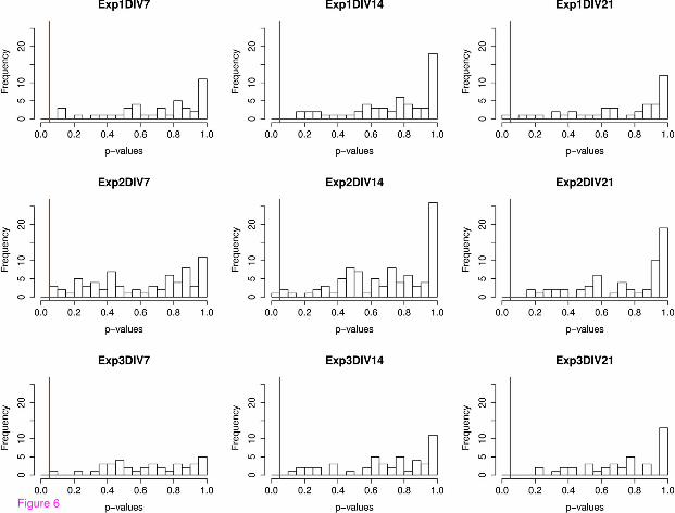
Figure 6

Figure 7

Additional files provided with this submission:

Additional file 1: 9646963309143235_add1.pdf, 50Khttp://www.biomedcentral.com/imedia/1501100695108806/supp1.pdfAdditional file 2: 9646963309143235_add2.pdf, 32Khttp://www.biomedcentral.com/imedia/1651367278108806/supp2.pdf