Blood Vessel Segmentation from Retinal Images

Anil Maharjan

Master's thesis

School of Computing

Computer Science

June 2016

i

UNIVERSITY OF EASTERN FINLAND, Faculty of Science and Forestry, Joensuu School of Computing

Computer Science

Anil Maharjan: Blood Vessel Segmentation from Retinal Images

Master’s Thesis, 88 p., 4 appendixes (18 p.)

Supervisor of the Master’s Thesis: PhD Pauli Fӓlt

June 2016

ii

Preface

This thesis was done at the School of Computing, University of Eastern Finland dur-

ing the spring 2016. I would like to express my gratitude to all the people who have

helped me in completing this thesis.

First of all, I would like to thank my supervisor PhD Pauli Fält for providing guide-

lines and suggestions. His valuable comments and help related to subject matters are

the key to successfully complete this work. I would also like to thank Professor

Markku Hauta-Kasari from University of Eastern Finland and Virpi Alhainen from

Natural Resources Institute Finland (Luke) for their motivation and suggestions to

accomplish my thesis.

Finally, I would like to express my gratitude to my parents and friends for their con-

stant love and support.

Forssa, June 2016

Anil Maharjan

iii

Abstract

Automatic retinal blood vessel segmentation algorithms are important procedures in

the computer aided diagnosis in the field of ophthalmology. They help to produce

useful information for the diagnosis and monitoring of eye diseases such as diabetic

retinopathy, hypertension and glaucoma.

In this work, different state-of-art methods for retinal blood vessel segmentation

were implemented and analyzed. Firstly, a supervised method based on gray level

and moment invariant features with neural network was explored. The other algo-

rithms taken into consideration were an unsupervised method based on gray-level co-

occurrence matrix with local entropy and a matched filtering method based on first

order derivative of Gaussian. During the work, two publicly available image data-

bases DRIVE and STARE were utilized for evaluating the performance of the algo-

rithms which includes sensitivity, specificity, accuracy, positive predictive value and

negative predictive value. The accuracies of the algorithms based on supervised and

unsupervised methods were 0.935 and 0.950 compared to corresponding values from

literature, which are 0.948 and 0.975, respectively. The matched filtering based

method produced same accuracy as in the literature, i.e., 0.941.

Although the accuracies of all implemented blood vessel segmentation methods were

close to the corresponding values given in the literature the sensitivities were lower

for all the algorithms which lead to smaller number of correctly classified vessels

from retinal images. Based on the results achieved, the algorithms have potential to

be accepted for practical use, after modest improvements are done in order to get

better segmentation of retinal blood vessels as well as the background.

Keywords: Retinal vessel segmentation, retinal image, performance measure, su-

pervised method, unsupervised method, matched filtering.

iv

List of abbreviations

Acc Accuracy

CPU Central processing unit

DRIVE Digital Retinal Images for Vessel Extraction (retinal image database)

FDOG First-order derivative of Gaussian

FOV Field of view

FPR False positive rate

GB Gigabyte

GHz Gigahertz

GLCM Gray-level co-occurrence matrix

GMM Gaussian mixture model

GPU Graphical processing unit

JPEG Joint photographic experts group image format

JRE Joint relative entropy

kNN K-nearest neighbors algorithm

MF Matched filter

NN Neural network

Npv Negative predictive value

OR Logical OR operation

PC Personal computer

PCA Principal component analysis

PCNN Pulse coupled neural network

PPM Portable pixel map image format

Ppv Positive predictive value

RACAL Radius based clustering algorithm

RAM Random access memory

RGB Red, green and blue color space

Se Sensitivity

SIMD Single instruction multiple data

Sp Specificity

STARE STructured Analysis of the REtina (retinal image database)

SVM Support vector machine

TPR True positive rate

UI User interface

VLSI Very large-scale integration

v

Contents

1 Introduction .................................................................................................... 1

1.1 Background ......................................................................................... 1 1.2 Motivation ........................................................................................... 2 1.3 Research questions .............................................................................. 3 1.4 Structure of the thesis ......................................................................... 4

2 Materials and methods ................................................................................... 5

2.1 Structure of the human eye ................................................................. 5 2.2 Materials ............................................................................................. 6

2.3 Blood vessel segmentation classification ........................................... 7

2.4 Supervised methods ............................................................................ 9 2.4.1 Gray level and moment invariant based features with

neural network ......................................................................... 11 2.4.1.1 Preprocessing .............................................................. 12

2.4.1.2 Feature extraction ........................................................ 14 2.4.1.3 Classification ............................................................... 17

2.4.1.4 Post processing ............................................................ 19 2.4.2 Other supervised methods for retinal image

segmentation ............................................................................ 20

2.5 Unsupervised methods ...................................................................... 21 2.5.1 Local entropy and gray-level co-occurrence matrix................ 22

2.5.1.1 Blood vessel enhancement using matched filter ......... 23

2.5.1.2 Gray-level co-occurrence matrix computation ............ 24

2.5.1.3 Joint relative entropy thresholding .............................. 26 2.5.2 Other unsupervised methods for retinal image

segmentation ............................................................................ 28 2.6 Matched filtering ............................................................................... 29

2.6.1 First-order derivative of Gaussian ........................................... 30

2.6.2 Other matched filtering methods for retinal image

segmentation ............................................................................ 33

3 Implementation ............................................................................................. 35

3.1 Supervised method using gray-level and moment invariants

with neural network .......................................................................... 35 3.2 Unsupervised method using local entropy and gray-level

co-occurrence matrix ........................................................................ 40

3.3 Matched filter using first order derivative of Gaussian .................... 42

4 Results .......................................................................................................... 47

5 Conclusion .................................................................................................... 60

vi

Appendices

Appendix A: Images showing segmentation results obtained from different blood

vessel segmentation algorithms

Appendix B: Matlab codes for supervised method using gray-level and moment

invariants with neural network

Appendix C: Matlab codes for unsupervised method using local entropy and gray-

level co-occurrence matrix

Appendix D: Matlab codes for matched filtering method using first order derivative

of Gaussian

1

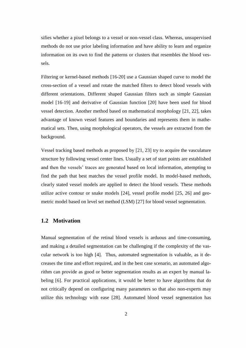
1 Introduction

Retina is the tissue lining the interior surface of the eye which contains the light-

sensitive cells (photoreceptors). Photoreceptors convert light into neural signals that

are carried to the brain through the optic nerves. In order to record the condition of

the retina, an image of the retina (fundus image) can be obtained. A fundus camera

system (retinal microscope) is usually used for capturing retinal images. Retinal im-

age contains essential diagnostic information which assists in determining whether

the retina is healthy or unhealthy.

Retinal images have been widely used for diagnosing vascular and non-vascular pa-

thology in medical society [1]. Retinal images provide information on the changes in

retinal vascular structure, which are common in diseases such as diabetes, occlusion,

glaucoma, hypertension, cardiovascular disease and stroke [2, 3]. These diseases

usually change reflectivity, tortuosity, and patterns of blood vessels [4]. For example,

hypertension changes the branching angle or tortuosity of vessels [5] and diabetic

retinopathy can lead to neovascularization i.e., development of new blood vessels. If

left untreated, these medical conditions can cause sight degradation or even blindness

[6]. The early exposure of these changes is important for taking preventive measure

and hence, the major vision loss can be prevented [7].

Automatic segmentation of retinal blood vessels from retinal images would be a

powerful tool for medical diagnostics. For this purpose, the segmentation method

used should be as accurate and reliable as possible. The main aim of segmentation is

to differentiate an object of interest and the background from an image.

1.1 Background

Several methods for the segmentation of retinal image have been reported in litera-

ture. Based on machine learning methods, retinal blood vessel segmentation can be

divided into two groups: supervised methods [1, 8-11] and unsupervised methods

[12-15]. Supervised methods are based on the prior labeling information which clas-

2

sifies whether a pixel belongs to a vessel or non-vessel class. Whereas, unsupervised

methods do not use prior labeling information and have ability to learn and organize

information on its own to find the patterns or clusters that resembles the blood ves-

sels.

Filtering or kernel-based methods [16-20] use a Gaussian shaped curve to model the

cross-section of a vessel and rotate the matched filters to detect blood vessels with

different orientations. Different shaped Gaussian filters such as simple Gaussian

model [16-19] and derivative of Gaussian function [20] have been used for blood

vessel detection. Another method based on mathematical morphology [21, 22], takes

advantage of known vessel features and boundaries and represents them in mathe-

matical sets. Then, using morphological operators, the vessels are extracted from the

background.

Vessel tracking based methods as proposed by [21, 23] try to acquire the vasculature

structure by following vessel center lines. Usually a set of start points are established

and then the vessels’ traces are generated based on local information, attempting to

find the path that best matches the vessel profile model. In model-based methods,

clearly stated vessel models are applied to detect the blood vessels. These methods

utilize active contour or snake models [24], vessel profile model [25, 26] and geo-

metric model based on level set method (LSM) [27] for blood vessel segmentation.

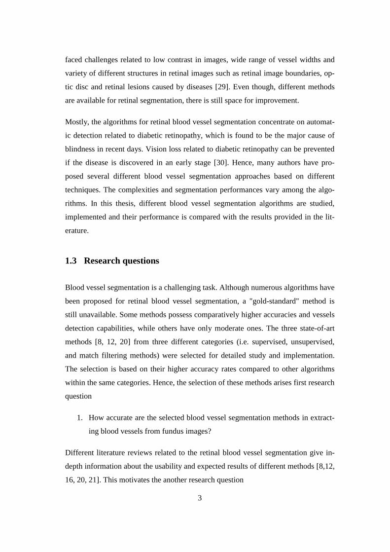
1.2 Motivation

Manual segmentation of the retinal blood vessels is arduous and time-consuming,

and making a detailed segmentation can be challenging if the complexity of the vas-

cular network is too high [4]. Thus, automated segmentation is valuable, as it de-

creases the time and effort required, and in the best case scenario, an automated algo-

rithm can provide as good or better segmentation results as an expert by manual la-

beling [6]. For practical applications, it would be better to have algorithms that do

not critically depend on configuring many parameters so that also non-experts may

utilize this technology with ease [28]. Automated blood vessel segmentation has

3

faced challenges related to low contrast in images, wide range of vessel widths and

variety of different structures in retinal images such as retinal image boundaries, op-

tic disc and retinal lesions caused by diseases [29]. Even though, different methods

are available for retinal segmentation, there is still space for improvement.

Mostly, the algorithms for retinal blood vessel segmentation concentrate on automat-

ic detection related to diabetic retinopathy, which is found to be the major cause of

blindness in recent days. Vision loss related to diabetic retinopathy can be prevented

if the disease is discovered in an early stage [30]. Hence, many authors have pro-

posed several different blood vessel segmentation approaches based on different

techniques. The complexities and segmentation performances vary among the algo-

rithms. In this thesis, different blood vessel segmentation algorithms are studied,

implemented and their performance is compared with the results provided in the lit-

erature.

1.3 Research questions

Blood vessel segmentation is a challenging task. Although numerous algorithms have

been proposed for retinal blood vessel segmentation, a "gold-standard" method is

still unavailable. Some methods possess comparatively higher accuracies and vessels

detection capabilities, while others have only moderate ones. The three state-of-art

methods [8, 12, 20] from three different categories (i.e. supervised, unsupervised,

and match filtering methods) were selected for detailed study and implementation.

The selection is based on their higher accuracy rates compared to other algorithms

within the same categories. Hence, the selection of these methods arises first research

question

1. How accurate are the selected blood vessel segmentation methods in extract-

ing blood vessels from fundus images?

Different literature reviews related to the retinal blood vessel segmentation give in-

depth information about the usability and expected results of different methods [8,12,

16, 20, 21]. This motivates the another research question

4

2. Are automated blood vessel extraction methods trustworthy compared to

manual segmentation done by experts?

The main goal of this thesis is to answer the research questions.

1.4 Structure of the thesis

Chapter 2 presents the physiological background related to the structure of the hu-

man eye and the functionality of its components. It also includes the materials used

for evaluating the algorithms that were implemented during the study of different

retinal vessel segmentation methods. It is followed by brief introduction of different

types of vessel segmentation methods proposed by different authors. Furthermore,

the chapter explains the three different categories for vessel segmentation methods:

supervised, unsupervised and matched filtering along with detailed explanation of

one method from each category.

Chapter 3 contains the detailed processes that were followed during the implementa-

tion of three different vessel segmentation methods. It includes the algorithms’ work-

flow followed by the calculation of their performance measures.

Chapter 4 describes the results obtained from the implemented algorithms and also

compares the corresponding performance measures with the original authors’ results.

Chapter 5 presents the thesis' conclusions based on the experimental results and also

the achievements from the study.

5

2 Materials and methods

2.1 Structure of the human eye

Human eye is the light-sensitive organ that enables one to see the surrounding envi-

ronment. It can be compared to a camera in a sense that the image is formed on the

retina of eye while in a traditional camera the image is formed on a film. The cornea

and the crystalline lens of the human eye are equivalent to the lens of a camera and

the iris of the eye works like the diaphragm of a camera, which controls the amount

of light reaching the retina by adjusting the size of pupil [31]. The light passing

through cornea, pupil and the lens reaches the retina at the back of the eye, which

contains the light sensitive photoreceptors. The image formed on the retina is trans-

formed into electrical impulses and carried to the brain through the optic nerves,

where the signals are processed and the sensation of vision is generated [32]. The

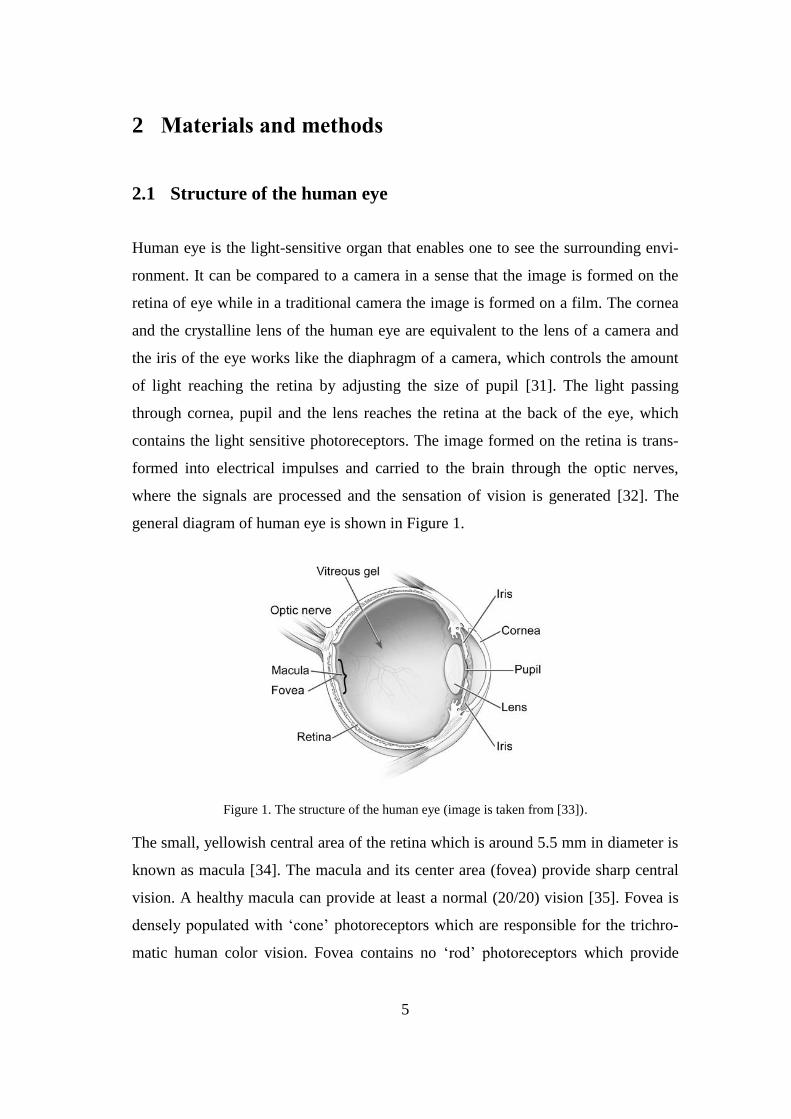
general diagram of human eye is shown in Figure 1.

Figure 1. The structure of the human eye (image is taken from [33]).

The small, yellowish central area of the retina which is around 5.5 mm in diameter is

known as macula [34]. The macula and its center area (fovea) provide sharp central

vision. A healthy macula can provide at least a normal (20/20) vision [35]. Fovea is

densely populated with ‘cone’ photoreceptors which are responsible for the trichro-

matic human color vision. Fovea contains no ‘rod’ photoreceptors which provide

6

information on brightness. The L-, M- and S-cone cells are sensitive to long, middle,

and short wavelength ranges in the visible part of the electromagnetic spectrum (i.e.,

380-780 nm), respectively, whereas rod cells provide no color information [34].

Optic disc is the visible part of the optic nerve where the optic nerve fibers and blood

vessels enter the eye. It does not contain any rod or cone photoreceptors, so it cannot

respond to light. Thus, it is also called a blind spot. The retinal arteries and veins

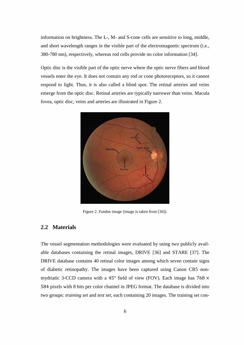
emerge from the optic disc. Retinal arteries are typically narrower than veins. Macula

fovea, optic disc, veins and arteries are illustrated in Figure 2.

Figure 2. Fundus image (image is taken from [36]).

2.2 Materials

The vessel segmentation methodologies were evaluated by using two publicly avail-

able databases containing the retinal images, DRIVE [36] and STARE [37]. The

DRIVE database contains 40 retinal color images among which seven contain signs

of diabetic retinopathy. The images have been captured using Canon CR5 non-

mydriatic 3-CCD camera with a 45° field of view (FOV). Each image has 768 ×

584 pixels with 8 bits per color channel in JPEG format. The database is divided into

two groups: training set and test set, each containing 20 images. The training set con-

7

tains color fundus images, the FOV masks for the images, and a set of manually

segmented monochrome (black and white) ground truth images. The test set contains

color fundus images, the FOV masks for the images, and two set of manually seg-

mented monochrome ground truth images by two different specialists. The ground

truth images of the first observer were used for measuring the performance of algo-

rithms.

The STARE database for blood vessel segmentation contains 20 color retinal images

among which ten contain pathology. The images have been taken using TopCon

TRV-50 camera with 35° FOV. Each image has 700 × 605 pixels with 8 bits per

color channel in PPM format. This database does not have separate training and test

sets as in DRIVE. It also contains two sets of manually segmented monochrome

ground truth images by two different specialists. The manually segmented images by

the first human observer were used as the ground truth for evaluating the perfor-

mance of the algorithms.

2.3 Blood vessel segmentation classification

There are several techniques for blood vessel segmentation and diagnosis of diseases

related to retina. Different authors have categorized those methods in different way.

In [21], the authors divided the retinal vessel segmentation into seven main catego-

ries; (1) pattern recognition techniques, (2) matched filtering, (3) mathematical mor-

phology, (4) multiscale approaches, (5) vessel tracking, (6) model based approaches,

and (7) parallel/hardware based approaches. Pattern recognition deals with classifica-

tion of retinal blood vessels and non-vessels together with background, based on key

features. This approach has two methods; supervised and unsupervised. If a priori

information is used to determine a pixel as a vessel or not, then that method is super-

vised, otherwise it is unsupervised method. Matched filtering uses convolution of

two dimensional kernels, which is designed to model a feature at some position and

orientation, with the retinal image and detect vessels by maximizing the responses of

kernels used [2, 4]. Mathematical morphology deals with the mathematical theory of

8

representing shapes like features, boundaries, etc. using sets. Mainly two morpholog-

ical operators; erosion and dilution, are used for applying structuring element to the

images. Two algorithms; Top hat and watershed transformations are popularly used

in medical image segmentation [21]. The combination of multiscale enhancement,

fuzzy filter and watershed transformation is used to extract vessels from retinal im-

age [22]. As the vessel moves away from the optic disc, its diameter decreases. The

idea behind multiscale approach is to use the vessel’s width to determine blood ves-

sels having varying width at different scales [21]. Many of the multiscale algorithms

are based on the vessel enhancement filter which is described by Frangi et al. [38].

And in [39], the vessel detection is obtained from fast discrete curvelet transform and

multi-structure mathematical morphology. Vessel tracking method segments a vessel

between two points by identifying vessel center line rather than entire vessels at once

[21, 23]. In this method, the tracing of the vessel, which seems like a line, is done by

using local information and by following vessel edges. Model based approach uses

fully and clearly expressed vessel models to extract blood vessels. The models like

snake or active contour model [25], multi-concavity modelling method [26], Hessi-

an-based technique [40] are some of the methods used in this approach. Parallel

hardware based approach is mainly for fast and real time performance, and imple-

mentation is done in hardware chips. The implementation of this approach for real

time image processing is done in VLSI chip by representing cellular neural network

[41]. In [42], morphological operations and convolutions are implemented together

with arithmetic and logical operations to extract blood vessels in single instruction

multiple data (SIMD) parallel processor array.

According to [4], vessel segmentation methods are grouped into three categories; (1)

pixel processing-based, (2) tracking-based, and (3) model-based approaches. Pixel

processing-based approach measures features for every pixel in an image and classi-

fies each pixel in either vessel or non-vessel class. It includes two processes: initial

enhancement of the image by applying convolution and secondly adaptive threshold-

ing and morphological operations followed by classification of vessel pixels. Pattern

recognition based, matched filtering, and multiscale based approaches mentioned in

9

[21] have resemblance with pixel processing-based method. While tracking-based

and model-based approaches are similar to that as mentioned in [21].

Another authors [2] have categorized vessel segmentation into three different meth-

ods; (1) kernel-based, (2) tracking based and (3) classifier-based. The kernel-based

method consists matched filtering, and mathematical morphology, while tracking

based is same as mentioned in [21]. Pattern recognition based approach as referred in

[21] is similar to the classifier-based method. This shows that even different authors

have different way of classifying the blood vessel segmentation, the main idea re-

mains same. Some authors want to elaborate the classification by defining detail

characteristics per approach while others combined two or more characteristics to

form a single approach and briefing the number of approaches.

Pattern recognition-based approaches like supervised and unsupervised methods, and

matched filtering-based methods are explained in detail in the following sections.

2.4 Supervised methods

Pattern recognition is the process of classifying input data into objects or classes by

the recognition and representation of patterns it contains and their relationships [43,

44]. It includes measurement of the object to identify attributes, extraction of features

for the defining attributes, and comparison with known patterns to determine the

class-memberships of objects; based on which classification is done. Pattern recogni-

tion is used in countless applications, such as computer aided design (CAD), in med-

ical science, speech recognition, optical character recognition (OCR), finger print

and face detection, and retinal blood vessel segmentation [43, 45]. It is generally

categorized according to the classification procedures. Classification is the procedure

for arranging pixels and assigning them to particular categories. The features used for

characterization of pixels can be texture, size, gray band value, etc. A set of extracted

features is called a feature vector. The general procedure used in classification is as

follows:

10

i. Classification classes definition: Depending upon the objective and

characteristics of the image data, the classes into which the pixels are

to be assigned, are determined.

ii. Feature selection: The features like texture, gray band value, etc. are

selected for classification.

iii. Characterize the classes in terms of the selected features: Usually two

sets of data with known class-memberships are defined; one for train-

ing and other for testing the classifier.

iv. Defining the parameters (if any) required for the classifier: The pa-

rameters or appropriate decision rules, required by the particular clas-

sification algorithm are determined using the training data.

v. Perform classification: Using the trained classifier (e.g., a maximum

likelihood classifier, or a minimum distance classifier), and the class

decision rules, the testing data are classified to the classes.

vi. Result evaluation: The accuracy and reliability of the classifier are

evaluated based on the test data classification results.

Based on the classification method, pattern recognition can be either supervised or

unsupervised [43]. Supervised classification is the procedure in which user interac-

tion is required: user defines the decision rules for each class/pixels or provides train-

ing data for each class/pixels to guide the classification. It uses supervised learning

algorithm for creating a classifier, based on training data from different object clas-

ses. The input data are provided to the classifier, which assigns the appropriate label

for each input. Whereas unsupervised method attempts to identify the patterns or

clusters from the input dataset without predefined classification rules [46]. It learns

and organizes information on its own to find the proper solution [47].

In blood vessel segmentation, the supervised method is based on pixel classification,

which utilizes the a priori labeling information to determine whether a pixel belongs

to a vessel or non-vessel. All pixels in image are classified into vessel or non-vessel

class by the classifier. In image classification, the training data is considered to rep-

resent the classes of interest. The quality of training data can significantly influence

11

the performance of an algorithm and thus, the classification accuracy [48], which

suggests to choose proper training data. Feature extraction and the selection of pa-

rameters for the classier are also critical because they assist in determining the accu-

racy and overall result of the classification algorithm. The classifiers are trained by

supervised learning with manually processed and segmented ground truth image [8,

21]. The ground truth image is precise and usually marked by an expert or ophthal-

mologist. Different kinds of classifiers, such as neural networks, Bayesian classifier,

support vector machine etc., have been used for improving classification [49, 50].

Similarly, various feature vectors have been used in supervised methods for blood

vessel segmentation, like Gabor feature, line operator, gray-level and moment invari-

ants [1, 8, 9]. The preceding section describes a supervised method of blood vessel

segmentation using gray-level and moment invariant based features with neural net-

work as classifier.

2.4.1 Gray level and moment invariant based features with neural net-

work

The term ‘gray-level’ refers to the intensity of a particular pixel in the image. In

segmentation of image using supervised method, the sequence of gray levels of pix-

el’s neighbors can be used as a feature vector [51]. A feature vector is a vector that

contains information describing an object's important characteristics. Image moments

and moment invariants could help in object recognition and its analysis [52]. Mo-

ment invariants use the idea of describing the objects by a set of measurable quanti-

ties called invariants that are unresponsive to particular deformations and that pro-

vide enough information to distinguish among objects belonging to different classes.

The image processing technique that uses gray level and moment invariants based

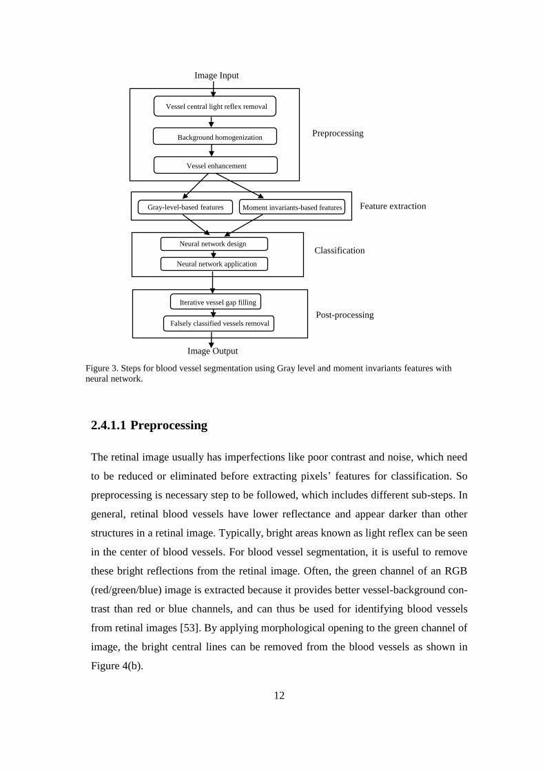
features with neural network can be explained in four different stages (see Figure 3):

Preprocessing of retinal image for gray level homogenization and blood vessel en-

hancement, feature extraction, classification of pixel to label it as vessel or non-

vessel, and post-processing for removing falsely detected isolated vessel pixels [8].

12

2.4.1.1 Preprocessing

The retinal image usually has imperfections like poor contrast and noise, which need

to be reduced or eliminated before extracting pixels’ features for classification. So

preprocessing is necessary step to be followed, which includes different sub-steps. In

general, retinal blood vessels have lower reflectance and appear darker than other

structures in a retinal image. Typically, bright areas known as light reflex can be seen

in the center of blood vessels. For blood vessel segmentation, it is useful to remove

these bright reflections from the retinal image. Often, the green channel of an RGB

(red/green/blue) image is extracted because it provides better vessel-background con-

trast than red or blue channels, and can thus be used for identifying blood vessels

from retinal images [53]. By applying morphological opening to the green channel of

image, the bright central lines can be removed from the blood vessels as shown in

Figure 4(b).

Figure 3. Steps for blood vessel segmentation using Gray level and moment invariants features with

neural network.

Background homogenization

Image Input

Image Output

Preprocessing

Vessel central light reflex removal

Vessel enhancement

Gray-level-based features Feature extraction Moment invariants-based features

Neural network application

Classification Neural network design

Falsely classified vessels removal Post-processing

Iterative vessel gap filling

13

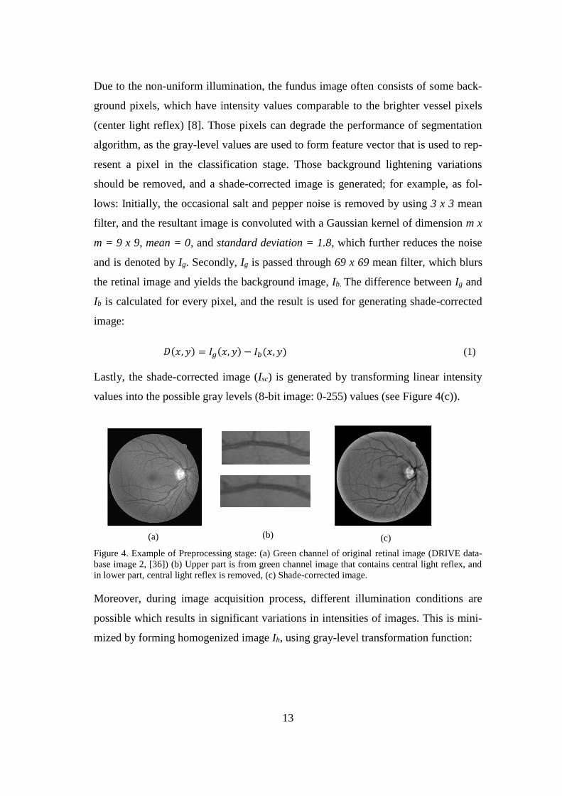
Due to the non-uniform illumination, the fundus image often consists of some back-

ground pixels, which have intensity values comparable to the brighter vessel pixels

(center light reflex) [8]. Those pixels can degrade the performance of segmentation

algorithm, as the gray-level values are used to form feature vector that is used to rep-

resent a pixel in the classification stage. Those background lightening variations

should be removed, and a shade-corrected image is generated; for example, as fol-

lows: Initially, the occasional salt and pepper noise is removed by using 3 x 3 mean

filter, and the resultant image is convoluted with a Gaussian kernel of dimension m x

m = 9 x 9, mean = 0, and standard deviation = 1.8, which further reduces the noise

and is denoted by Ig. Secondly, Ig is passed through 69 x 69 mean filter, which blurs

the retinal image and yields the background image, Ib. The difference between Ig and

Ib is calculated for every pixel, and the result is used for generating shade-corrected

image:

𝐷(𝑥, 𝑦) = 𝐼𝑔(𝑥, 𝑦) − 𝐼𝑏(𝑥, 𝑦) (1)

Lastly, the shade-corrected image (Isc) is generated by transforming linear intensity

values into the possible gray levels (8-bit image: 0-255) values (see Figure 4(c)).

Figure 4. Example of Preprocessing stage: (a) Green channel of original retinal image (DRIVE data-

base image 2, [36]) (b) Upper part is from green channel image that contains central light reflex, and

in lower part, central light reflex is removed, (c) Shade-corrected image.

Moreover, during image acquisition process, different illumination conditions are

possible which results in significant variations in intensities of images. This is mini-

mized by forming homogenized image Ih, using gray-level transformation function:

(a) (b) (c)

14

(a) (b) (c)

𝑔Output = {

0, 𝑖𝑓 𝑔 < 0255, 𝑖𝑓 𝑔 > 255𝑔, 𝑜𝑡ℎ𝑒𝑟𝑤𝑖𝑠𝑒

(2)

where,

𝑔 = 𝑔Input + 128 − 𝑔Input_max (3)

Here, 𝑔Input and 𝑔Output are the gray level variables of input (Isc) and output (Ih) re-

spectively and 𝑔Input_max is the gray level value of input (Isc), which has highest

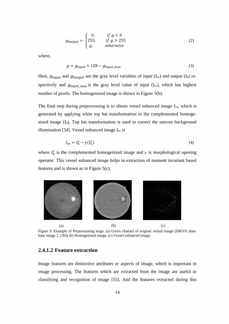
number of pixels. The homogenized image is shown in Figure 5(b).

The final step during preprocessing is to obtain vessel enhanced image Ive, which is

generated by applying white top hat transformation to the complemented homoge-

nized image (Ih). Top hat transformation is used to correct the uneven background

illumination [54]. Vessel enhanced image Ive is

𝐼𝑣𝑒 = 𝐼ℎ𝑐 − 𝛾(𝐼ℎ

𝑐) (4)

where 𝐼ℎ𝑐 is the complemented homogenized image and 𝛾 is morphological opening

operator. This vessel enhanced image helps in extraction of moment invariant based

features and is shown as in Figure 5(c).

Figure 5. Example of Preprocessing stage: (a) Green channel of original retinal image (DRIVE data-

base image 2, [36]) (b) Homogenized image, (c) Vessel-enhanced image.

2.4.1.2 Feature extraction

Image features are distinctive attributes or aspects of image, which is important in

image processing. The features which are extracted from the image are useful in

classifying and recognition of image [55]. And the features extracted during this

15

phase helps in classifying pixels whether it belongs to vessel or not. Two different

kind of features; gray level based features and moment invariant based features are

extracted [8].

A. Gray level based features

Blood vessels are usually darker than background in the green channel image. So the

gray levels of pixels on vessels are smaller than gray levels of other pixels in a local

area. This statistical gray level information of vessels can be used to obtain the fea-

tures from retinal image [56]. Gray level features in retinal image are based on the

difference between the gray level in vessel pixel and a statistical value of its sur-

rounding local pixels. The homogenized image, Ih is used to generate a set of gray

level based features for each image pixel (x, y) by operating only on a small image

area (window) centered at (x, y). The feature vectors are calculated as:

𝑓1(𝑥, 𝑦) = 𝐼ℎ(𝑥, 𝑦) − 𝑚𝑖𝑛(𝑠,𝑡)𝜖𝑆𝑥,𝑦

9{𝐼ℎ(𝑠, 𝑡)} (5)

𝑓2(𝑥, 𝑦) = 𝑚𝑎𝑥(𝑠,𝑡)𝜖𝑆𝑥,𝑦

9{𝐼ℎ(𝑠, 𝑡)} − 𝐼ℎ(𝑥, 𝑦) (6)

𝑓3(𝑥, 𝑦) = 𝐼ℎ(𝑥, 𝑦) − 𝑚𝑒𝑎𝑛(𝑠,𝑡)𝜖𝑆𝑥,𝑦

9{𝐼ℎ(𝑠, 𝑡)} (7)

𝑓4(𝑥, 𝑦) = 𝑠𝑡𝑑(𝑠,𝑡)𝜖𝑆𝑥,𝑦

9{𝐼ℎ(𝑠, 𝑡)} (8)

𝑓5(𝑥, 𝑦) = 𝐼ℎ(𝑥, 𝑦) (9)

where 𝑆𝑥,𝑦𝑤 is set of co-ordinates having window size of 𝑤 × 𝑤 and window center

point at (x, y).

B. Moment invariant based features

Invariant moments have had a great impact on image recognition or classification

and have been widely used as features for recognition in many areas of image pro-

cessing. They are popular because of having property which does not change with

rotation, scale and translation [57, 58]. Hence invariant moments are computed for

each separate block and the result is compared with the target image blocks for find-

ing the similarity.

16

The two-dimensional moment of order (𝑝 + 𝑞) for image 𝑓(𝑥, 𝑦) can be obtained as:

𝑚𝑝𝑞 = ∑ ∑ 𝑥𝑝𝑦𝑞𝑓(𝑥, 𝑦)𝑦𝑥 where p, q = 0, 1, 2 … (10)

Consider a small block of image defined by region 𝑆𝑥,𝑦17 from vessel enhanced image

Ive and a pixel as (𝑥, 𝑦), having window size of 17 × 17. Then its moment is calculat-

ed as

𝑚𝑝𝑞 = ∑ ∑ 𝑖𝑝𝑗𝑞𝐼𝑣𝑒𝑆𝑥,𝑦17

(𝑖, 𝑗)𝑗𝑖 (11)

where 𝐼𝑣𝑒𝑆𝑥,𝑦17

is the gray level at point (𝑖, 𝑗). And the central moment is defined as

µ𝑝𝑞 = ∑ ∑ (𝑖 − 𝑖)𝑝( 𝑗 − 𝑗)𝑞𝐼𝑣𝑒

𝑆𝑥,𝑦17

(𝑖, 𝑗)𝑗𝑖 (12)

where, 𝑖 =𝑚10

𝑚00 and 𝑗 =

𝑚01

𝑚00 are the centroid of the image. Similarly, the normalized

central moment is defined as

𝜂𝑝𝑞 =𝜇𝑝𝑞

(𝜇00)(𝑝+𝑞2+1)

where 𝑝 + 𝑞 = 2, 3, … (13)

The concept of moment invariant is introduced by Hu, and based on normalized cen-

tral moments, a set of seven different moment invariants are defined, among which

first two are enough to obtain optimal performance reducing the computation com-

plexity [8, 59]. The two moments taken into consideration are:

∅1 = 𝜂20 + 𝜂02 (14)

∅2 = (𝜂20 + 𝜂02)2 + 4𝜂11

2 (15)

According to [8], the moment invariants obtained from 𝐼𝑣𝑒𝑆𝑥,𝑦17

are not useful to define

the central pixel of the sub-image as a vessel or non-vessel. So the new sub-image Ihu

is generated to surpass that problem. Ihu is produced by multiplying the original ves-

sel enhanced sub-image 𝐼𝑣𝑒𝑆𝑥,𝑦17

with a Gaussian filter of window size=17 × 17, mean=0

and variance=1.72. Hence, the new sub-image is described as:

𝐼ℎ𝑢(𝑖, 𝑗) = 𝐼𝑣𝑒𝑆𝑥,𝑦17

(𝑖, 𝑗) × 𝐺0,1.7217 (𝑖, 𝑗) (16)

17

Using Ihu, first and second moment invariants are generated. So these moment invari-

ant features for pixel located at (𝑥, 𝑦) can be obtained as:

𝑓6(𝑥, 𝑦) = |𝑙𝑜𝑔 (∅1)| (17)

𝑓7(𝑥, 𝑦) = |𝑙𝑜𝑔 (∅2)| (18)

2.4.1.3 Classification

The seven features for each pixel obtained from feature extraction process is charac-

terized by a vector in a seven-dimensional feature space as:

𝐹(𝑥, 𝑦) = [𝑓1(𝑥, 𝑦), 𝑓2(𝑥, 𝑦), … , 𝑓7(𝑥, 𝑦)] (19)

These features are used in classification process in which every candidate pixel is

classified as either a vessel pixel (C1) or non-vessel pixel (C2). According to [8], the

use of a linear classifier results in relatively poor ability to separate classes in vessel

segmentation, which creates a need for a non-linear classifier. There are few non-

linear classifiers like Bayesian classifier, support vector machine, kNN classifier and

neural network. For implementation of blood vessel segmentation, a neural network

(NN) is used as a non-linear classifier.

Neural network is defined as a computing system consisting of a number of simple,

interconnected processing elements, which respond to and process information from

external inputs [60]. Neural networks are typically organized in layers consisting of

a number of interconnected 'nodes', which contain an 'activation function' [61]. Input

data are presented to the network via the 'input layer', which transfers input data to

one or more 'hidden layers' where the actual processing is done via a system of

weighted 'connections'. The 'output layer' gets result from hidden layer and transfer

that output for corresponding agent.

The classification process for blood vessel segmentation is divided into two phases:

Neural network design, and neural network application. A multilayer feedforward

network with adequate neurons in a single hidden layer can approximate any func-

tion, provided the activation function of the neurons satisfies some general con-

18

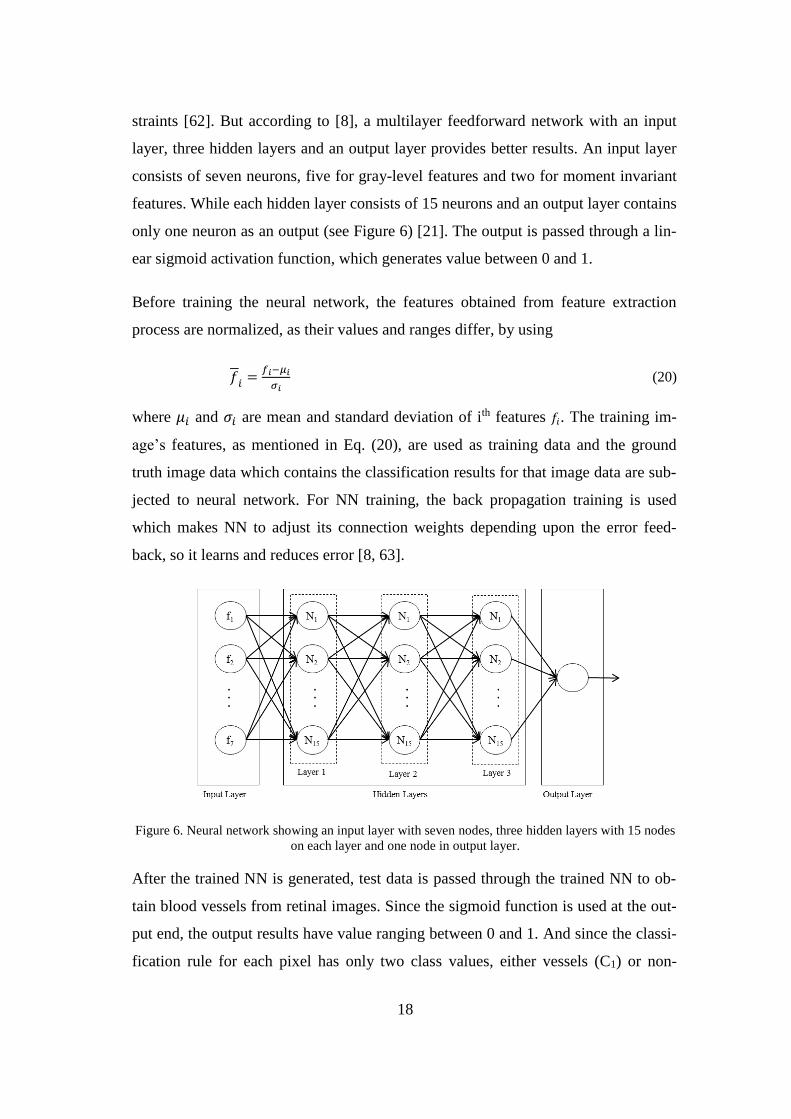
straints [62]. But according to [8], a multilayer feedforward network with an input

layer, three hidden layers and an output layer provides better results. An input layer

consists of seven neurons, five for gray-level features and two for moment invariant

features. While each hidden layer consists of 15 neurons and an output layer contains

only one neuron as an output (see Figure 6) [21]. The output is passed through a lin-

ear sigmoid activation function, which generates value between 0 and 1.

Before training the neural network, the features obtained from feature extraction

process are normalized, as their values and ranges differ, by using

𝑓𝑖 =𝑓𝑖−𝜇𝑖

𝜎𝑖 (20)

where 𝜇𝑖 and 𝜎𝑖 are mean and standard deviation of ith features 𝑓𝑖. The training im-

age’s features, as mentioned in Eq. (20), are used as training data and the ground

truth image data which contains the classification results for that image data are sub-

jected to neural network. For NN training, the back propagation training is used

which makes NN to adjust its connection weights depending upon the error feed-

back, so it learns and reduces error [8, 63].

Figure 6. Neural network showing an input layer with seven nodes, three hidden layers with 15 nodes

on each layer and one node in output layer.

After the trained NN is generated, test data is passed through the trained NN to ob-

tain blood vessels from retinal images. Since the sigmoid function is used at the out-

put end, the output results have value ranging between 0 and 1. And since the classi-

fication rule for each pixel has only two class values, either vessels (C1) or non-

19

vessels (C2), thresholding is required. Considering a threshold Th and applying it on

each candidate pixel produces a classification output image Ico so that classes C1 and

C2 are associated to gray levels 255 and 0, respectively, as follows:

𝐼𝑐𝑜(𝑥, 𝑦) = {255 (≡ 𝐶1), 𝑖𝑓 𝑝(𝐶1|𝐹(𝑥, 𝑦)) > 𝑇ℎ0 (≡ 𝐶2), 𝑂𝑡ℎ𝑒𝑟𝑤𝑖𝑠𝑒

(21)

where 𝑝(𝐶1|𝐹(𝑥, 𝑦)) denotes the probability of a candidate pixel (𝑥, 𝑦) to belong to a

vessel class C1 as explained by the feature vector 𝐹(𝑥, 𝑦) [8]. The thresholded image

is shown in Figure 5(b).

2.4.1.4 Post processing

The post processing stage is another import operation to obtain better and accurate

segmentation. Usually during this stage, the noise produced by the classification

stage is removed. It is divided into two steps: iterative filling of pixel gaps in detect-

ed blood vessels, and falsely detected isolated vessel pixel removal.

The vessels might have gaps which are vessel pixels but have been classified as non-

vessels. By applying iterative filling procedure these gaps can be filled. This is done

by considering that each candidate pixel with at least six neighbors classified as ves-

sel points must also belong to a vessel [8, 29]. The next step is to remove falsely

classified vessel pixels, for which first get the number of pixels in each connected

region, and reclassify to those pixels by labeling as a non-vessel each pixel that has

less than 25 vessel-pixels in a region connected to it [8]. By increasing or decreasing

the limiting pixel count, the accuracy and sensitivity of the blood vessel segmenta-

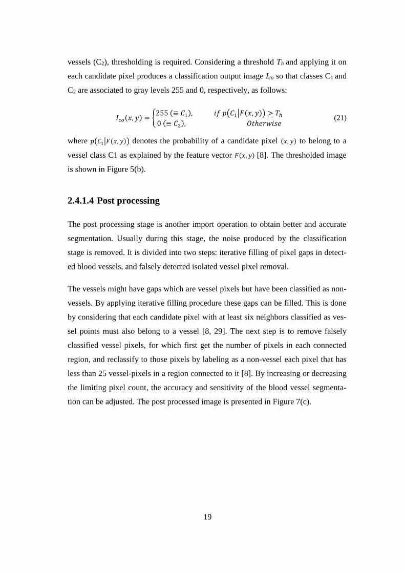
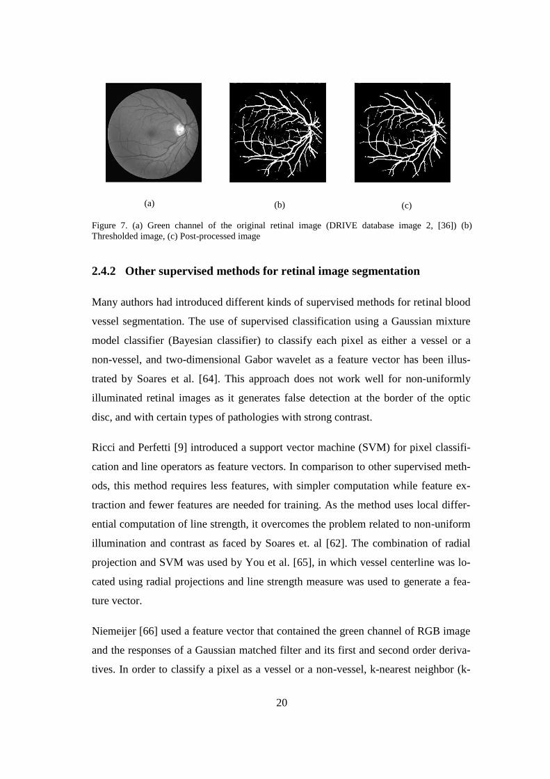
tion can be adjusted. The post processed image is presented in Figure 7(c).

20

Figure 7. (a) Green channel of the original retinal image (DRIVE database image 2, [36]) (b)

Thresholded image, (c) Post-processed image

2.4.2 Other supervised methods for retinal image segmentation

Many authors had introduced different kinds of supervised methods for retinal blood

vessel segmentation. The use of supervised classification using a Gaussian mixture

model classifier (Bayesian classifier) to classify each pixel as either a vessel or a

non-vessel, and two-dimensional Gabor wavelet as a feature vector has been illus-

trated by Soares et al. [64]. This approach does not work well for non-uniformly

illuminated retinal images as it generates false detection at the border of the optic

disc, and with certain types of pathologies with strong contrast.

Ricci and Perfetti [9] introduced a support vector machine (SVM) for pixel classifi-

cation and line operators as feature vectors. In comparison to other supervised meth-

ods, this method requires less features, with simpler computation while feature ex-

traction and fewer features are needed for training. As the method uses local differ-

ential computation of line strength, it overcomes the problem related to non-uniform

illumination and contrast as faced by Soares et. al [62]. The combination of radial

projection and SVM was used by You et al. [65], in which vessel centerline was lo-

cated using radial projections and line strength measure was used to generate a fea-

ture vector.

Niemeijer [66] used a feature vector that contained the green channel of RGB image

and the responses of a Gaussian matched filter and its first and second order deriva-

tives. In order to classify a pixel as a vessel or a non-vessel, k-nearest neighbor (k-

(a) (b) (c)

21

NN) classifier was used. Staal [10] also used a k-NN classifier for classification in

his ridge based vessel segmentation algorithm. The features used are based on the

ridge of the image and total of 27 features are used to form a feature vector.

A supervised method using an AdaBoost classifier was introduced by Lupascu et at.

[46]. They used a relatively large number of features, about 41, to form a feature

vector. The features include various vessel related descriptions like, local (pixel’s

intensity and Hessian-based measures), structural (vessel’s geometric structures),

and spatial (gray-level profile approximated by Gaussian curve).

Shadgar and Osareh use a multiscale Gabor filter for vessel identification and princi-

pal component analysis (PCA) for feature extraction [47]. The classification algo-

rithms like Gaussian mixture model (GMM) and SVM are used for classifying a

pixel as vessel or non-vessel. Besides the algorithms mentioned above, there are also

other supervised blood vessel segmentation methods, which are not included here.

2.5 Unsupervised methods

Unsupervised learning is another method used in pattern recognition. In supervised

methods, class-labels of the training data are known beforehand. In unsupervised

methods, neither the classes nor the assignments of the training data to the classes are

known. Instead, unsupervised methods try to identify patterns or clusters in the train-

ing data [46]. Unsupervised methods have an ability to learn and organize infor-

mation but do not give error signals that could be used to evaluate the performances

of the given potential solutions [47]. Sometimes this can be advantageous, since it

enables the algorithm to look back for patterns that have not been previously consid-

ered [67].

The goal of unsupervised learning is to model the underlying structure or distribution

in the data in order to learn more about the data. Algorithms are left on their own to

discover and present interesting structures in the data. Sometimes unsupervised

learning provides superior, and broadly usable, alternative to established methods,

especially for problems that haven't been solved clearly by supervised method [68].

22

Unsupervised methods have been used in various applications such as Natural Lan-

guage Processing (NLP), data mining, fraud analysis, remote sensing image classifi-

cation, object recognition, and also retinal image segmentation.

In retinal blood vessel segmentation, the unsupervised classification tries to find fun-

damental patterns of blood vessels, which is used to determine whether a pixel is

vessel or non-vessel. In this method, the training data or gold standard image does

not help directly to design the algorithm [21]. Various authors have proposed differ-

ent retinal image segmentation methods. The method by Villalobos-Castaldi et al.

[12] using local entropy information with gray-level co-occurrence matrix (GLCM)

has yielded relatively better results than others. The reported results for accuracy,

sensitivity and specificity are 0.9759, 0.9648 and 0.9759 respectively, for DRIVE

retinal images.

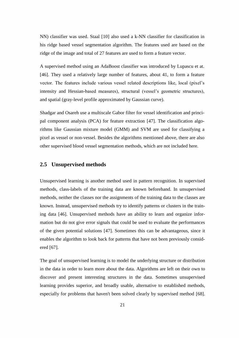
2.5.1 Local entropy and gray-level co-occurrence matrix

In general, a single generally acknowledged vessel segmentation algorithm does not

exist due to the unique properties of each acquisition technique. Every segmentation

method has some challenges in detecting vessels precisely when applied alone. In

this method, a combination of two methods, matched filtering and co-occurrence

matrix with entropy thresholding, are applied to detect retinal blood vessels. Hence,

the retinal image segmentation, as described by Villalobos-Castaldi et al. [12], based

on local entropy and gray-level co-occurrence matrix is divided into three different

stages: blood vessel enhancement using matched filter, gray-level co-occurrence ma-

trix computation, and segmentation of extracted blood vessel using joint relative en-

tropy thresholding. The workflow of this method is illustrated in Figure 8.

23

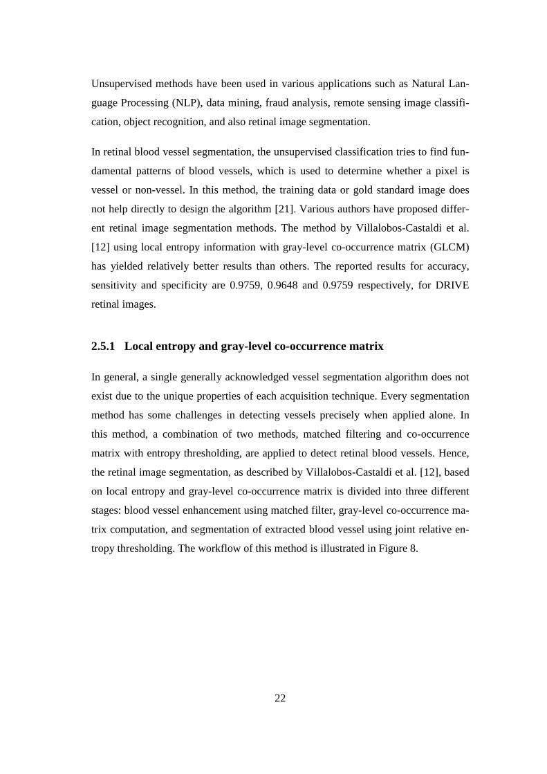
2.5.1.1 Blood vessel enhancement using matched filter

Since blood vessels appear darker compared to the background, the vessels should be

enhanced before proceeding. Hence, the green channel of an RGB retinal image is

extracted as it provides better vessel-background contrast than red or blue channels

[53]. The green channel image is used for further processing with matched filter.

Usually blood vessels do not have absolute step edges and gray-level intensity profile

varies in every blood vessel [69]. The intensity profile of a cross section of a blood

vessel can be modeled by a Gaussian shaped curve [17], which is shown in Figure

13(a). Hence, a matched filter can be used for the detection of piecewise linear seg-

ments of blood vessels in retinal images [70]. The two dimensional matched filter

kernel is convolved with the green channel retinal image to enhance the blood ves-

sels. According to Chaudhuri et al. [17], the two dimensional Gaussian matched filter

can be expressed as:

𝑓(𝑥, 𝑦) = − 𝑒𝑥𝑝 (−𝑥2

2𝜎2) ∀ |𝑦| ≤

𝐿

2 (22)

Input image

Blood vessel enhancement

Gray-level co-occurrence matrix computation

Green channel image

Joint relative entropy thresholding

Output image

Figure 8. Flowchart of unsupervised method of segmentation using joint relative entropy and co-

occurrence matrix.

24

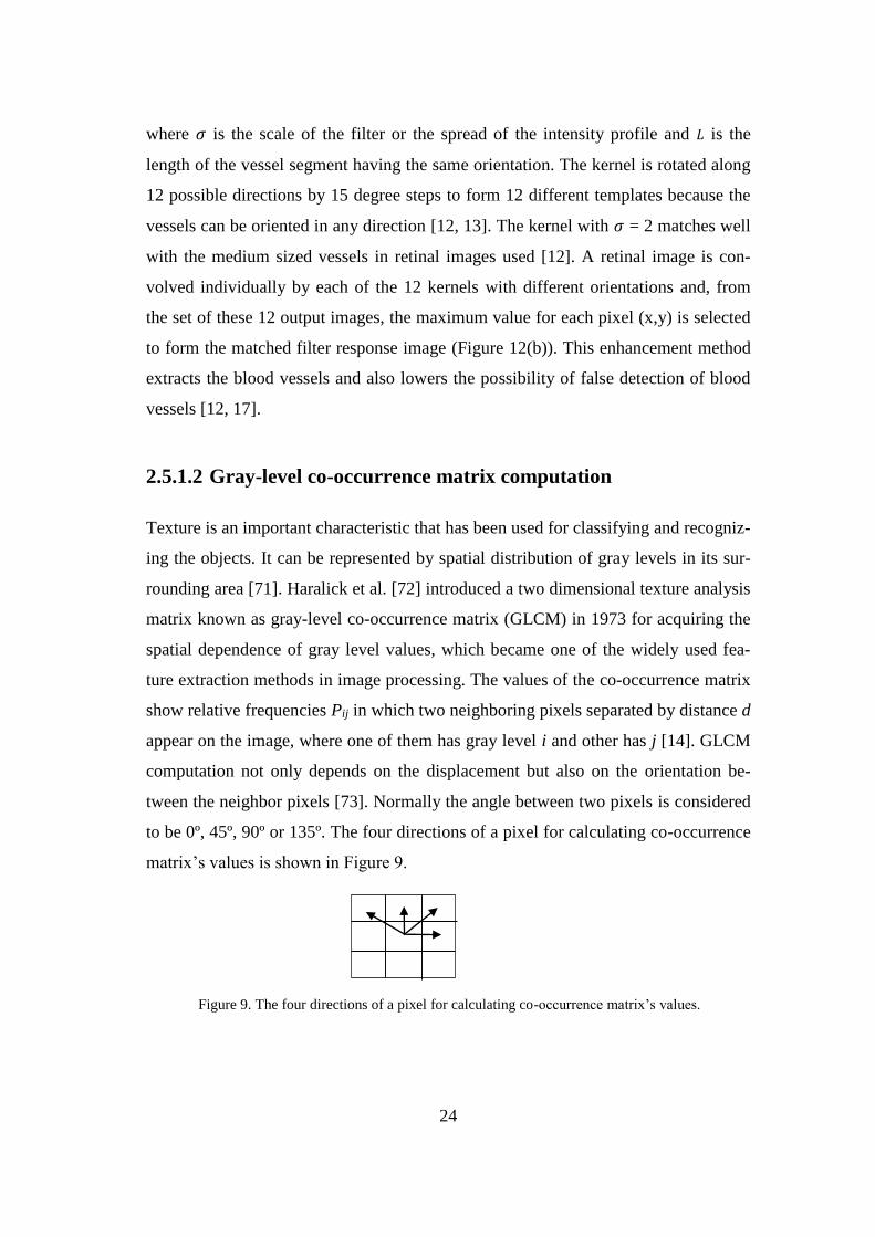
where 𝜎 is the scale of the filter or the spread of the intensity profile and 𝐿 is the

length of the vessel segment having the same orientation. The kernel is rotated along

12 possible directions by 15 degree steps to form 12 different templates because the

vessels can be oriented in any direction [12, 13]. The kernel with 𝜎 = 2 matches well

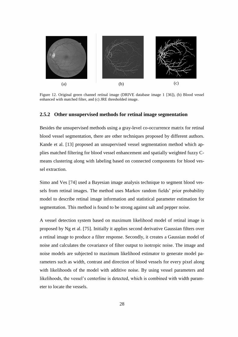
with the medium sized vessels in retinal images used [12]. A retinal image is con-

volved individually by each of the 12 kernels with different orientations and, from

the set of these 12 output images, the maximum value for each pixel (x,y) is selected

to form the matched filter response image (Figure 12(b)). This enhancement method

extracts the blood vessels and also lowers the possibility of false detection of blood

vessels [12, 17].

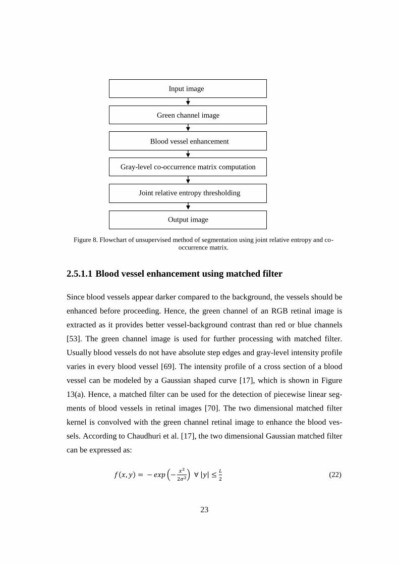
2.5.1.2 Gray-level co-occurrence matrix computation

Texture is an important characteristic that has been used for classifying and recogniz-

ing the objects. It can be represented by spatial distribution of gray levels in its sur-

rounding area [71]. Haralick et al. [72] introduced a two dimensional texture analysis

matrix known as gray-level co-occurrence matrix (GLCM) in 1973 for acquiring the

spatial dependence of gray level values, which became one of the widely used fea-

ture extraction methods in image processing. The values of the co-occurrence matrix

show relative frequencies Pij in which two neighboring pixels separated by distance d

appear on the image, where one of them has gray level i and other has j [14]. GLCM

computation not only depends on the displacement but also on the orientation be-

tween the neighbor pixels [73]. Normally the angle between two pixels is considered

to be 0º, 45º, 90º or 135º. The four directions of a pixel for calculating co-occurrence

matrix’s values is shown in Figure 9.

Figure 9. The four directions of a pixel for calculating co-occurrence matrix’s values.

25

Consider an image of size 𝑀 ×𝑁 with 𝐿 gray levels expressed by 𝐺 =

{0, 1, 2, … , 𝐿 − 1} and the gray level of pixel at location (𝑚, 𝑛) be 𝑓(𝑚, 𝑛). The co-

occurrence matrix of an image is a 𝐿 × 𝐿 square matrix, which can be denoted as

𝑊 = [𝑡𝑖𝑗]𝐿×𝐿, where 𝑡𝑖𝑗 is the number of transitions from gray level value 𝑖 to gray

level value 𝑗 [69]. The value of 𝑡𝑖𝑗 can be calculated as

𝑡𝑖𝑗 = ∑ ∑ 𝛿𝑚𝑛 𝑁𝑛=1

𝑀𝑚=1 (23)

where, 𝛿𝑚𝑛 =

{

1, 𝑖𝑓 {

𝑓(𝑚, 𝑛) = 𝑖 𝑎𝑛𝑑 𝑓(𝑚 + 1, 𝑛) = 𝑗 𝑎𝑛𝑑/𝑜𝑟

𝑓(𝑚, 𝑛) = 𝑖 𝑎𝑛𝑑 𝑓(𝑚, 𝑛 + 1) = 𝑗

0, 𝑜𝑡ℎ𝑒𝑟 𝑤𝑖𝑠𝑒

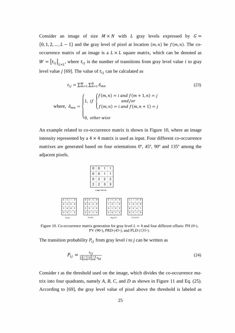
An example related to co-occurrence matrix is shown in Figure 10, where an image

intensity represented by a 4 × 4 matrix is used as input. Four different co-occurrence

matrixes are generated based on four orientations 0º, 45º, 90º and 135º among the

adjacent pixels.

The transition probability 𝑃𝑖𝑗 from gray level i to j can be written as

𝑃𝑖𝑗 =𝑡𝑖𝑗

∑ ∑ 𝑡𝑘𝑙 𝐿−1𝑙=0

𝐿−1𝑘=0

(24)

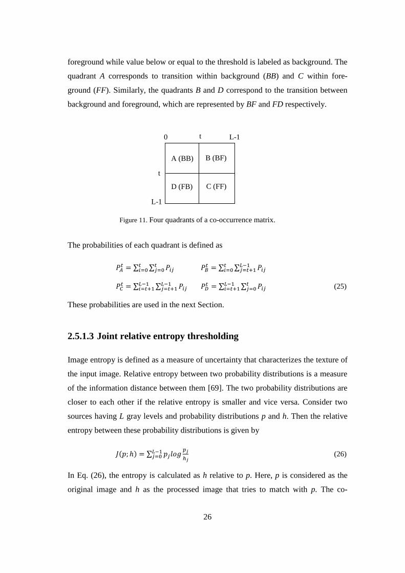
Consider t as the threshold used on the image, which divides the co-occurrence ma-

trix into four quadrants, namely A, B, C, and D as shown in Figure 11 and Eq. (25).

According to [69], the gray level value of pixel above the threshold is labeled as

Figure 10. Co-occurrence matrix generation for gray level 𝐿 = 4 and four different offsets: PH (0◦),

PV (90◦), PRD (45◦), and PLD (135◦).

26

foreground while value below or equal to the threshold is labeled as background. The

quadrant A corresponds to transition within background (BB) and C within fore-

ground (FF). Similarly, the quadrants B and D correspond to the transition between

background and foreground, which are represented by BF and FD respectively.

The probabilities of each quadrant is defined as

𝑃𝐴𝑡 = ∑ ∑ 𝑃𝑖𝑗

𝑡𝑗=0

𝑡𝑖=0 𝑃𝐵

𝑡 = ∑ ∑ 𝑃𝑖𝑗 𝐿−1𝑗=𝑡+1

𝑡𝑖=0

𝑃𝐶𝑡 = ∑ ∑ 𝑃𝑖𝑗

𝐿−1𝑗=𝑡+1

𝐿−1𝑖=𝑡+1 𝑃𝐷

𝑡 = ∑ ∑ 𝑃𝑖𝑗 𝑡𝑗=0

𝐿−1𝑖=𝑡+1 (25)

These probabilities are used in the next Section.

2.5.1.3 Joint relative entropy thresholding

Image entropy is defined as a measure of uncertainty that characterizes the texture of

the input image. Relative entropy between two probability distributions is a measure

of the information distance between them [69]. The two probability distributions are

closer to each other if the relative entropy is smaller and vice versa. Consider two

sources having L gray levels and probability distributions p and h. Then the relative

entropy between these probability distributions is given by

𝐽(𝑝; ℎ) = ∑ 𝑝𝑗𝑙𝑜𝑔𝑝𝑗

ℎ𝑗

𝐿−1𝑗=0 (26)

In Eq. (26), the entropy is calculated as h relative to p. Here, p is considered as the

original image and h as the processed image that tries to match with p. The co-

0 t

t

L-1

L-1

C (FF) D (FB)

A (BB) B (BF)

Figure 11. Four quadrants of a co-occurrence matrix.

27

occurrence matrix can be used to expand the first order relative entropy into second

order joint relative entropy (Eq. 27). Let t be the threshold value and ℎ𝑖𝑗𝑡 the transi-

tion probability of the thresholded image. Then the cell probabilities of the

thresholded image in all four quadrants are defined as

ℎ𝑖𝑗|𝐴𝑡 = 𝑞𝐴

𝑡 =𝑃𝐴𝑡

(𝑡+1)(𝑡+1) ℎ𝑖𝑗|𝐵

𝑡 = 𝑞𝐵𝑡 =

𝑃𝐵𝑡

(𝑡+1)(𝐿−𝑡−1)

ℎ𝑖𝑗|𝐶𝑡 = 𝑞𝐶

𝑡 =𝑃𝐶𝑡

(𝐿−𝑡−1)(𝐿−𝑡−1) ℎ𝑖𝑗|𝐷

𝑡 = 𝑞𝐷𝑡 =

𝑃𝐷𝑡

(𝐿−𝑡−1)(𝑡+1) (27)

Using Eq. (25) and Eq. (27), Eq. (26) can be expressed as

𝐽({𝑝𝑖𝑗}; {ℎ𝑖𝑗𝑡 }) = ∑ ∑ 𝑝𝑖𝑗

𝐿−1𝑗=0 𝑙𝑜𝑔

𝑝𝑖𝑗

ℎ𝑖𝑗𝑡

𝐿−1𝑖=0

= −𝐻({𝑝𝑖𝑗}) − ∑ 𝑝𝑖𝑗𝑙𝑜𝑔𝑖𝑗 ℎ𝑖𝑗𝑡

= −𝐻({𝑝𝑖𝑗}) − (𝑃𝐴𝑡𝑙𝑜𝑔𝑞𝐴

𝑡 + 𝑃𝐵𝑡 𝑙𝑜𝑔𝑞𝐵

𝑡 + 𝑃𝐶𝑡𝑙𝑜𝑔𝑞𝐶

𝑡 + 𝑃𝐷𝑡 𝑙𝑜𝑔𝑞𝐷

𝑡 ) (28)

where 𝐻({𝑝𝑖𝑗}) is the entropy of {𝑝𝑖𝑗}𝑖=0,𝑗=0𝐿−1,𝐿−1

, which is independent of threshold t

and is expressed as 𝐻({𝑝𝑖𝑗}) = −∑ ∑ 𝑝𝑖𝑗𝐿−1𝑗=0 𝑙𝑜𝑔𝑝𝑖𝑗

𝐿−1𝑖=0 . According to [69], the

proper threshold value for segmenting foreground (vessels) from background can be

obtained by taking quadrants B and D into consideration. Hence, only using

𝑃𝐵𝑡 𝑙𝑜𝑔𝑞𝐵

𝑡 + 𝑃𝐷𝑡 𝑙𝑜𝑔𝑞𝐷

𝑡 from Eq. (28) gives more effective edge detection. Therefore,

the joint relative entropy (JRE) threshold can be defined as

𝑡𝑗𝑟𝑒 = arg [min𝑡𝜖𝐺

𝐻𝑗𝑟𝑒(𝑡)] (29)

where,

𝐻𝑗𝑟𝑒(𝑡) = −(𝑃𝐵𝑡 𝑙𝑜𝑔𝑞𝐵

𝑡 + 𝑃𝐷𝑡 𝑙𝑜𝑔𝑞𝐷

𝑡 ) (30)

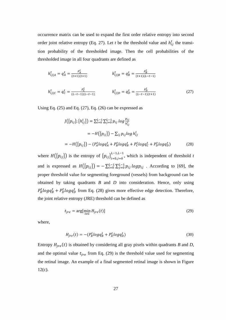
Entropy 𝐻𝑗𝑟𝑒(𝑡) is obtained by considering all gray pixels within quadrants B and D,

and the optimal value 𝑡𝑗𝑟𝑒 from Eq. (29) is the threshold value used for segmenting

the retinal image. An example of a final segmented retinal image is shown in Figure

12(c).

28

Figure 12. Original green channel retinal image (DRIVE database image 1 [36]), (b) Blood vessel

enhanced with matched filter, and (c) JRE thresholded image.

2.5.2 Other unsupervised methods for retinal image segmentation

Besides the unsupervised methods using a gray-level co-occurrence matrix for retinal

blood vessel segmentation, there are other techniques proposed by different authors.

Kande et al. [13] proposed an unsupervised vessel segmentation method which ap-

plies matched filtering for blood vessel enhancement and spatially weighted fuzzy C-

means clustering along with labeling based on connected components for blood ves-

sel extraction.

Simo and Ves [74] used a Bayesian image analysis technique to segment blood ves-

sels from retinal images. The method uses Markov random fields’ prior probability

model to describe retinal image information and statistical parameter estimation for

segmentation. This method is found to be strong against salt and pepper noise.

A vessel detection system based on maximum likelihood model of retinal image is

proposed by Ng et al. [75]. Initially it applies second derivative Gaussian filters over

a retinal image to produce a filter response. Secondly, it creates a Gaussian model of

noise and calculates the covariance of filter output to isotropic noise. The image and

noise models are subjected to maximum likelihood estimator to generate model pa-

rameters such as width, contrast and direction of blood vessels for every pixel along

with likelihoods of the model with additive noise. By using vessel parameters and

likelihoods, the vessel’s centerline is detected, which is combined with width param-

eter to locate the vessels.

(a) (b) (c)

29

Salem et al. [76] developed a radius based clustering algorithm (RACAL) that uses a

distance based rule to map the distributions of the image pixels. It uses features like

local maxima of the gradient magnitude and local maxima of large eigenvalue ob-

tained from a Hessian matrix. The method combines a clustering algorithm with a

partial supervision strategy.

2.6 Matched filtering

Retinal blood vessels can be detected using methods based on filter operators.

Matched filtering is a pattern matching algorithm based on the structural properties

of the object to be identified or recognized [16]. The expected appearance of a de-

sired signal or object can be described by a matched filter [19]. The use of matched

filter to detect retinal blood vessels has been carried out by Chaudhuri et al. [17],

which makes use of a priori knowledge that cross-section of vessels can be approxi-

mated by Gaussian function, which suggested that matching the blood vessels can be

done using a Gaussian shaped filter. According to Chaudhuri et al. [17], retinal blood

vessels possess three different characteristics:

● The blood vessels have small curvatures and may be approximated by piece-

wise linear segmentation.

● The width of blood vessel decreases when moving away from the optic disk.

● Due to lower reflectance of vessels in comparison to other retinal structures,

they seem to be darker compared to the background.

Using matched filtering, image’s features can be detected, which are most similar to

a predefined template [17]. In this method, blood vessels are assumed to be piece-

wise linear segments with cross sectional intensity changes similar to a predefined

kernel [18]. As blood vessels can have different spatial orientations, a set of kernels

is required to detect the vessels. An adequate number of kernels to detect vessels

with different orientations is considered to be 12, which are produced by rotating

each kernel by 15 degrees apart from the previous one [16, 17, 77]. The matched

filter kernel can be expressed as [20]:

30

𝐾(𝑥, 𝑦) =1

√2𝜋𝜎exp (−

𝑥2

2𝜎2) −𝑚 𝑓𝑜𝑟 |𝑥| ≤ 𝑡𝜎 , |𝑦| ≤

𝐿

2 (31)

where,

𝑚 =(∫

1

√2𝜋𝜎exp(−

𝑥2

2𝜎2)𝑑𝑥

𝑡𝜎

−𝑡𝜎)

(2𝑡𝜎) (32)

is the normalizing factor. And L is the length of the vessel segment having same

orientation and 𝜎 is the scale of filter or spread of intensity profile. Normalizing the

mean value of filter to 0 aids in removing smooth background after filtering. About

99% of the area under Gaussian curve lies within range of[−3𝜎, 3𝜎], hence the con-

stant, 𝑡 is set to value of 3. The parameter L is chosen based on the value of 𝜎. The

smaller the value of 𝜎, 𝐿 needs to be set relatively smaller as well, and vice versa.

According to [17], the best parameter values of L and 𝜎 which give maximum re-

sponse are at 𝐿 = 9 and 𝜎 = 2.

Since 12 different kernels, rotated at 15 degree steps, are enough for determining the

all possible vessels, every pixel of the image is convolved with these kernels. The

result obtained after examining all the pixels produces output image which consists

of dark pixels denoting non-vessels whereas bright pixels belong to the vessels [18].

According to Chaudhuri et al. [17], when both the kernel and vessel have same orien-

tation, then the pixel response is maximum.

2.6.1 First-order derivative of Gaussian

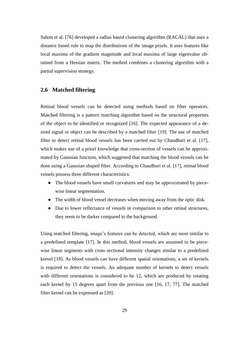
Matched filter (MF) has ability to respond to both the vessels’ and non-vessels’ edg-

es. This problem can be seen in Figures 13(a), (b1) and (b2), which show the re-

sponse of a MF to a Gaussian function (i.e. cross section of a vessel) and a step edge

(i.e. non-vessel). It is hard to separate vessels only by using MF because both vessels

and non-vessels will be detected after applying threshold over MF response. Hence,

an extra filter is also required along with MF, which in this case is the first-order

derivative of Gaussian (FDOG) filter [20].

31

Figure 13. Responses of the matched filter (MF) and the first-order derivative of Gaussian (FDOG) to

a Gaussian line cross section and an ideal step edge: (a) a Gaussian line cross-section and an ideal step

edge, (b-1) the MF and (b-2) its filter response, (c-1) the FDOG and (c-2) its filter response and (d)

the local mean of the response to the FDOG [20].

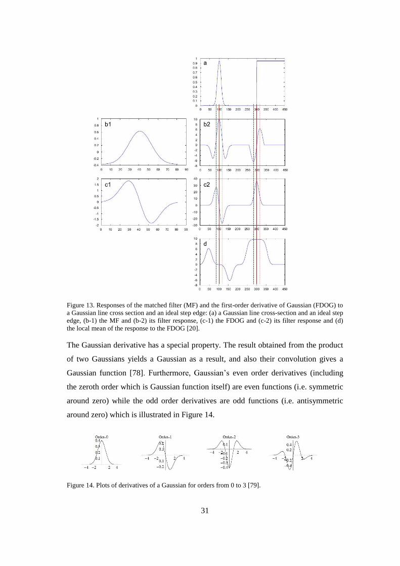
The Gaussian derivative has a special property. The result obtained from the product

of two Gaussians yields a Gaussian as a result, and also their convolution gives a

Gaussian function [78]. Furthermore, Gaussian’s even order derivatives (including

the zeroth order which is Gaussian function itself) are even functions (i.e. symmetric

around zero) while the odd order derivatives are odd functions (i.e. antisymmetric

around zero) which is illustrated in Figure 14.

Figure 14. Plots of derivatives of a Gaussian for orders from 0 to 3 [79].

32

Mathematically, the first order derivative of Gaussian matched filter, which is de-

fined in Eq. (31), can be written as

𝐾(𝑥, 𝑦) = −𝑥

√2𝜋𝜎3exp (−

𝑥2

2𝜎2) 𝑓𝑜𝑟 |𝑥| ≤ 𝑡𝜎 , |𝑦| ≤

𝐿

2 (33)

Figure 13 shows that the response of Gaussian function is strong, and positive for the

MF and anti-symmetric for FDOG. On the other hand, the non-vessel step edge’s

response for FDOG is strong and symmetric but anti-symmetric for MF [20]. If a

threshold T is applied to MF response, it detects both vessels and non-vessels, and

leads to wrong classification. Hence, the thresholding needs to be applied to the MF

response image but the threshold value is adjusted based on the image’s response to

FDOG [20].

Consider h as the MF response and d as FDOG response as illustrated in Figures 13

(b-2) and (c-2). The local mean of d, dm is the response obtained as the average of

neighboring pixels as shown in Figure 13 (d). Since the retinal image is filtered

twice, by MF and by FDOG, the two responses H and D are generated respectively.

And as the threshold value is adjusted using FDOG, the local mean of D can be cal-

culated by applying a mean filter over D as

𝐷𝑚 = 𝐷 ∗𝑊 (34)

where 𝑊 is a mean filter with a window size of 𝑤 × 𝑤. The local mean image 𝐷𝑚 is

normalized and denoted as ��𝑚, which is used to generate the threshold value. The

threshold value 𝑇 can be obtained by

𝑇 = (1 + ��𝑚)𝑇𝑐 (35)

where Tc is the reference threshold which is calculated as

𝑇𝑐 = 𝑐 × 𝜇𝐻 (36)

where 𝑐 is constant value that is usually between 2 and 3 and 𝜇𝐻 is the mean value of

the MF response H [20]. The threshold 𝑇 obtained in Eq. (35) is applied to H in order

to get final segmented image 𝐼𝐻, which can be presented as

33

𝐼𝐻 = {1 𝐻(𝑥, 𝑦) ≥ 𝑇(𝑥, 𝑦)

0 𝐻(𝑥, 𝑦) < 𝑇(𝑥, 𝑦) (37)

An example of the final segmented image along with original and ground truth imag-

es are illustrated in Figure 15.

Figure 15. (a) Original green channel retinal image (STARE database image 162 [37]), (b) Ground

truth image and (c) Blood vessels extracted using MF-FDOG.

2.6.2 Other matched filtering methods for retinal image segmentation

The first two-dimensional linear Gaussian filter used for the segmentation of retinal

blood vessels was proposed by Chauduri et al. [17]. The Gaussian filter or kernel is

rotated by 15 degree steps to match the different orientations of blood vessels. For

every pixel, the largest response value is selected and used as a threshold value to

segment the retinal blood vessels. Chauduri’s matched filter concept was improved

by Al-Rawi et al. [16] using an exhaustive search optimization technique. This meth-

(c)

(a) (b)

34

od finds the optimal matched filter size and threshold value which is applied to the

input retinal image and obtained segmented image.

Hoover et al. [19] used threshold probing technique on a matched filter response im-

age along with local and region-based features of a retinal image for segmentation.

This method analyzes the matched filter response image in pieces. With iterative

probing, a threshold is applied to each pixel and each pixel is classified as a vessel or

a non-vessel. The method produced approximately 75% true positive rate and also 15

times smaller false positive rate than the basic thresholding of matched filter re-

sponse.

The combination of a matched filter and an ANT colony algorithm for retinal image

segmentation is suggested by Cinsdikici and Aydin [80]. A preprocessed retinal im-

age is passed through a matched filter and ANT algorithm in parallel fashion and the

results are combined together. After applying length filtering over the result, the reti-

nal blood vessels are extracted.

Yao and Chen [81] proposed a two-dimensional Gaussian matched filter for blood

vessel enhancement. A pulse coupled neural network (PCNN) is applied for segmen-

tation which produces multiple results. Furthermore, among the number of segmenta-

tion results, the best results are selected by using a 2-D-Otsu algorithm. After analyz-

ing the local connectivity among the pixels, the final segmented retinal image is ob-

tained. There are also other methods related to retinal blood vessel segmentation

based on matched filtering technique, but they are not considered in the scope of this

thesis.

35

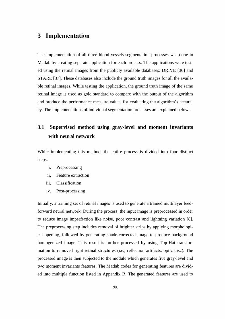
3 Implementation

The implementation of all three blood vessels segmentation processes was done in

Matlab by creating separate application for each process. The applications were test-

ed using the retinal images from the publicly available databases: DRIVE [36] and

STARE [37]. These databases also include the ground truth images for all the availa-

ble retinal images. While testing the application, the ground truth image of the same

retinal image is used as gold standard to compare with the output of the algorithm

and produce the performance measure values for evaluating the algorithm’s accura-

cy. The implementations of individual segmentation processes are explained below.

3.1 Supervised method using gray-level and moment invariants

with neural network

While implementing this method, the entire process is divided into four distinct

steps:

i. Preprocessing

ii. Feature extraction

iii. Classification

iv. Post-processing

Initially, a training set of retinal images is used to generate a trained multilayer feed-

forward neural network. During the process, the input image is preprocessed in order

to reduce image imperfection like noise, poor contrast and lightning variation [8].

The preprocessing step includes removal of brighter strips by applying morphologi-

cal opening, followed by generating shade-corrected image to produce background

homogenized image. This result is further processed by using Top-Hat transfor-

mation to remove bright retinal structures (i.e., reflection artifacts, optic disc). The

processed image is then subjected to the module which generates five gray-level and

two moment invariants features. The Matlab codes for generating features are divid-

ed into multiple function listed in Appendix B. The generated features are used to

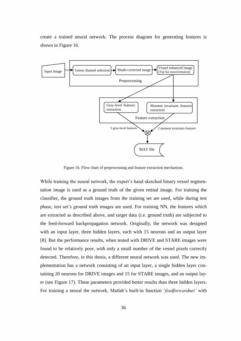
36

create a trained neural network. The process diagram for generating features is

shown in Figure 16.

While training the neural network, the expert’s hand sketched binary vessel segmen-

tation image is used as a ground truth of the given retinal image. For training the

classifier, the ground truth images from the training set are used, while during test

phase, test set’s ground truth images are used. For training NN, the features which

are extracted as described above, and target data (i.e. ground truth) are subjected to

the feed-forward backpropagation network. Originally, the network was designed

with an input layer, three hidden layers, each with 15 neurons and an output layer

[8]. But the performance results, when tested with DRIVE and STARE images were

found to be relatively poor, with only a small number of the vessel pixels correctly

detected. Therefore, in this thesis, a different neural network was used. The new im-

plementation has a network consisting of an input layer, a single hidden layer con-

taining 20 neurons for DRIVE images and 15 for STARE images, and an output lay-

er (see Figure 17). These parameters provided better results than three hidden layers.

For training a neural the network, Matlab’s built-in function ‘feedforwardnet’ with

Figure 16. Flow chart of preprocessing and feature extraction mechanism.

2 moment invariants features 5 gray-level features

Green channel selection Shade-corrected image Vessel enhanced image (Top hat transformation) Input image

Preprocessing

Feature extraction

Moment invariants features

extraction

Gray-level features

extraction

MAT file

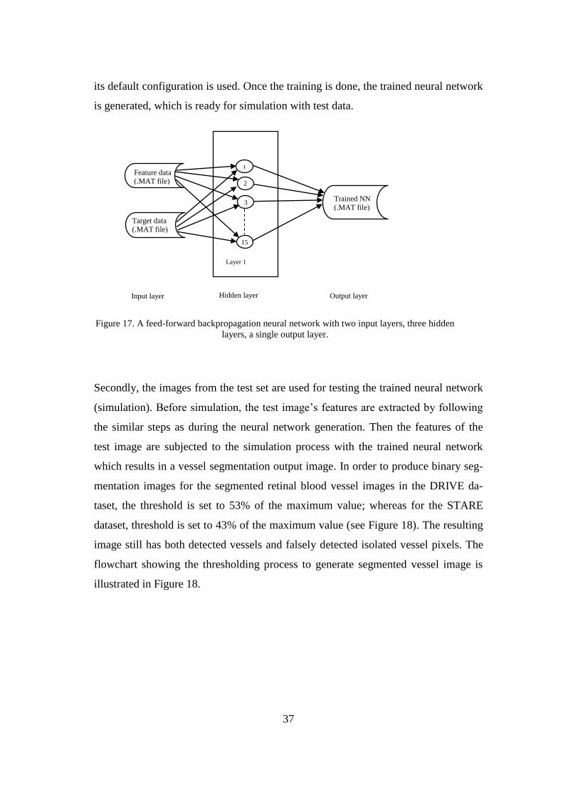
37

its default configuration is used. Once the training is done, the trained neural network

is generated, which is ready for simulation with test data.

Secondly, the images from the test set are used for testing the trained neural network

(simulation). Before simulation, the test image’s features are extracted by following

the similar steps as during the neural network generation. Then the features of the

test image are subjected to the simulation process with the trained neural network

which results in a vessel segmentation output image. In order to produce binary seg-

mentation images for the segmented retinal blood vessel images in the DRIVE da-

taset, the threshold is set to 53% of the maximum value; whereas for the STARE

dataset, threshold is set to 43% of the maximum value (see Figure 18). The resulting

image still has both detected vessels and falsely detected isolated vessel pixels. The

flowchart showing the thresholding process to generate segmented vessel image is

illustrated in Figure 18.

Input layer Hidden layer Output layer

Feature data (.MAT file)

Trained NN

(.MAT file)

Target data (.MAT file)

1

2

3

15

Layer 1

Figure 17. A feed-forward backpropagation neural network with two input layers, three hidden

layers, a single output layer.

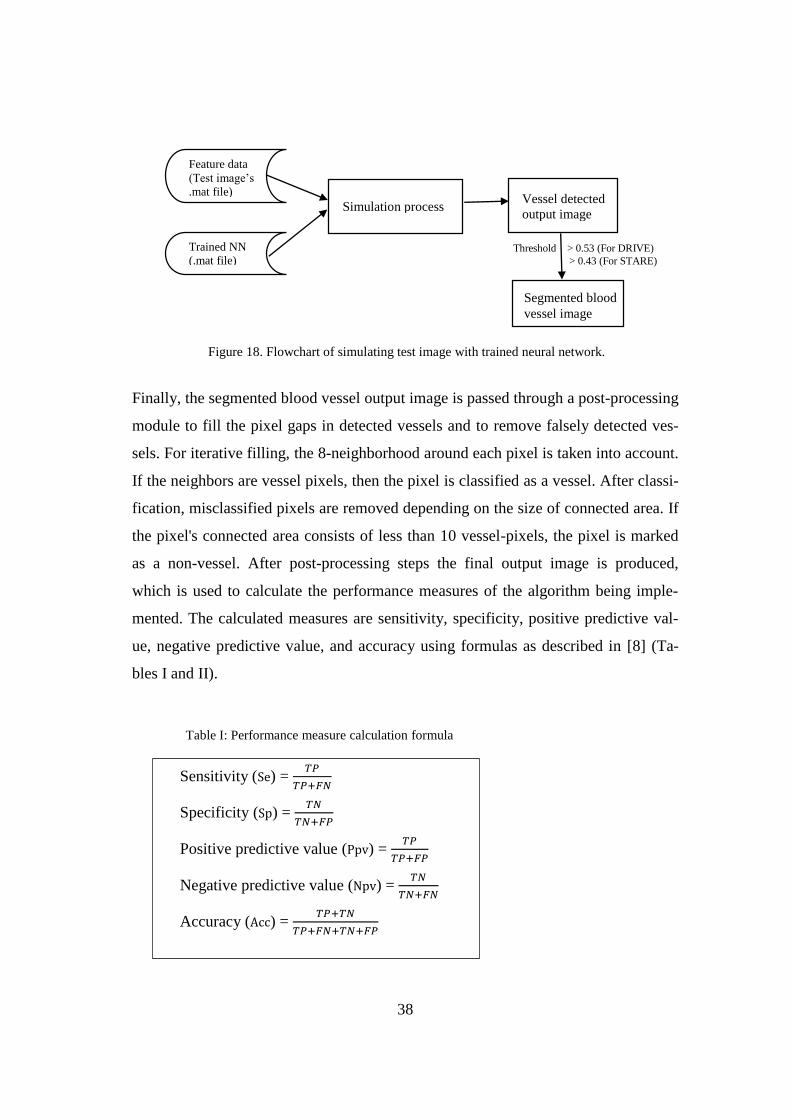
38

Finally, the segmented blood vessel output image is passed through a post-processing

module to fill the pixel gaps in detected vessels and to remove falsely detected ves-

sels. For iterative filling, the 8-neighborhood around each pixel is taken into account.

If the neighbors are vessel pixels, then the pixel is classified as a vessel. After classi-

fication, misclassified pixels are removed depending on the size of connected area. If

the pixel's connected area consists of less than 10 vessel-pixels, the pixel is marked

as a non-vessel. After post-processing steps the final output image is produced,

which is used to calculate the performance measures of the algorithm being imple-

mented. The calculated measures are sensitivity, specificity, positive predictive val-

ue, negative predictive value, and accuracy using formulas as described in [8] (Ta-

bles I and II).

Sensitivity (Se) = 𝑇𝑃

𝑇𝑃+𝐹𝑁

Specificity (Sp) = 𝑇𝑁

𝑇𝑁+𝐹𝑃

Positive predictive value (Ppv) = 𝑇𝑃

𝑇𝑃+𝐹𝑃

Negative predictive value (Npv) = 𝑇𝑁

𝑇𝑁+𝐹𝑁

Accuracy (Acc) = 𝑇𝑃+𝑇𝑁

𝑇𝑃+𝐹𝑁+𝑇𝑁+𝐹𝑃

Figure 18. Flowchart of simulating test image with trained neural network.

Table I: Performance measure calculation formula

Simulation process

Threshold > 0.53 (For DRIVE)

> 0.43 (For STARE)

Feature data

(Test image’s

.mat file)

Trained NN

(.mat file)

Vessel detected

output image

Segmented blood

vessel image

39

where,

Table II: Vessel classification [8].

Vessel present Vessel absent

Vessel detected True Positive (TP) False Positive (FP)

Vessel not detected False Negative (FN) True Negative (TN)

Sensitivity (Se) and specificity (Sp) are the ratios of correctly classified vessels and

non-vessels respectively. While Positive predictive value (Ppv) is the ratio of pixels

correctly classified as vessel pixel and negative predictive value (Npv) is the ratio of

pixels correctly classified as background. Accuracy is measured as the ratio of cor-

rectly classified pixels to the total number of pixels in field of view (FOV) [8]. The

function for calculating performance measures is implemented in Matlab code as

listed in Appendix B.

During implementation, the training and test datasets were taken from same database.

For example, the training set data from DRIVE database were used to generate a

trained NN and test set data were used for testing. Similarly, for STARE database, its

own training set and test set data were used for obtaining a trained NN and for test-

ing. Two training set images, one from DRIVE and STARE databases were also

combined to form a single training image and used for generating a trained NN. The

test result from this approach did not give any significant improvement in the result.

While training, the learning rate is also varied to get better results. The value of 5%

for learning rate gave better results than higher values, which obviously increased the

time required for training a NN. In general, the time requirement for training a NN

was around half an hour for 5 % learning rate. The test results, more specifically ac-

curacy and sensitivity, of DRIVE image dataset are comparatively better than for

STARE image dataset (see Table III and IV).

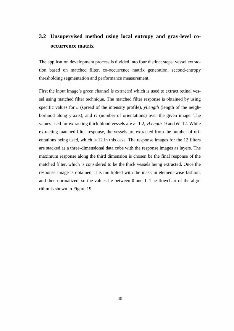
40

3.2 Unsupervised method using local entropy and gray-level co-

occurrence matrix

The application development process is divided into four distinct steps: vessel extrac-

tion based on matched filter, co-occurrence matrix generation, second-entropy

thresholding segmentation and performance measurement.

First the input image’s green channel is extracted which is used to extract retinal ves-

sel using matched filter technique. The matched filter response is obtained by using

specific values for σ (spread of the intensity profile), yLength (length of the neigh-

borhood along y-axis), and ϴ (number of orientations) over the given image. The

values used for extracting thick blood vessels are σ=1.2, yLength=9 and ϴ=12. While

extracting matched filter response, the vessels are extracted from the number of ori-

entations being used, which is 12 in this case. The response images for the 12 filters

are stacked as a three-dimensional data cube with the response images as layers. The

maximum response along the third dimension is chosen be the final response of the

matched filter, which is considered to be the thick vessels being extracted. Once the

response image is obtained, it is multiplied with the mask in element-wise fashion,

and then normalized, so the values lie between 0 and 1. The flowchart of the algo-

rithm is shown in Figure 19.

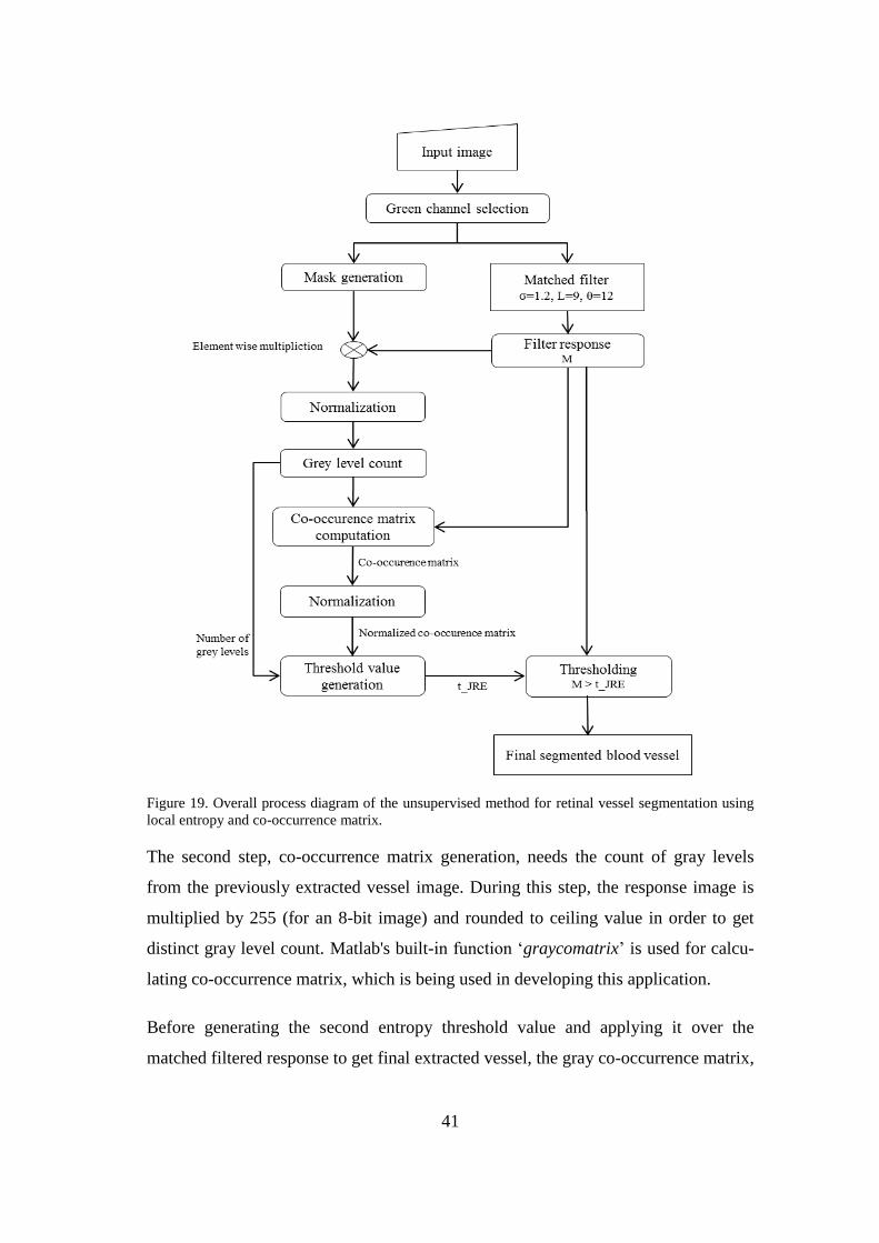
41

Figure 19. Overall process diagram of the unsupervised method for retinal vessel segmentation using

local entropy and co-occurrence matrix.

The second step, co-occurrence matrix generation, needs the count of gray levels

from the previously extracted vessel image. During this step, the response image is

multiplied by 255 (for an 8-bit image) and rounded to ceiling value in order to get

distinct gray level count. Matlab's built-in function ‘graycomatrix’ is used for calcu-

lating co-occurrence matrix, which is being used in developing this application.

Before generating the second entropy threshold value and applying it over the

matched filtered response to get final extracted vessel, the gray co-occurrence matrix,

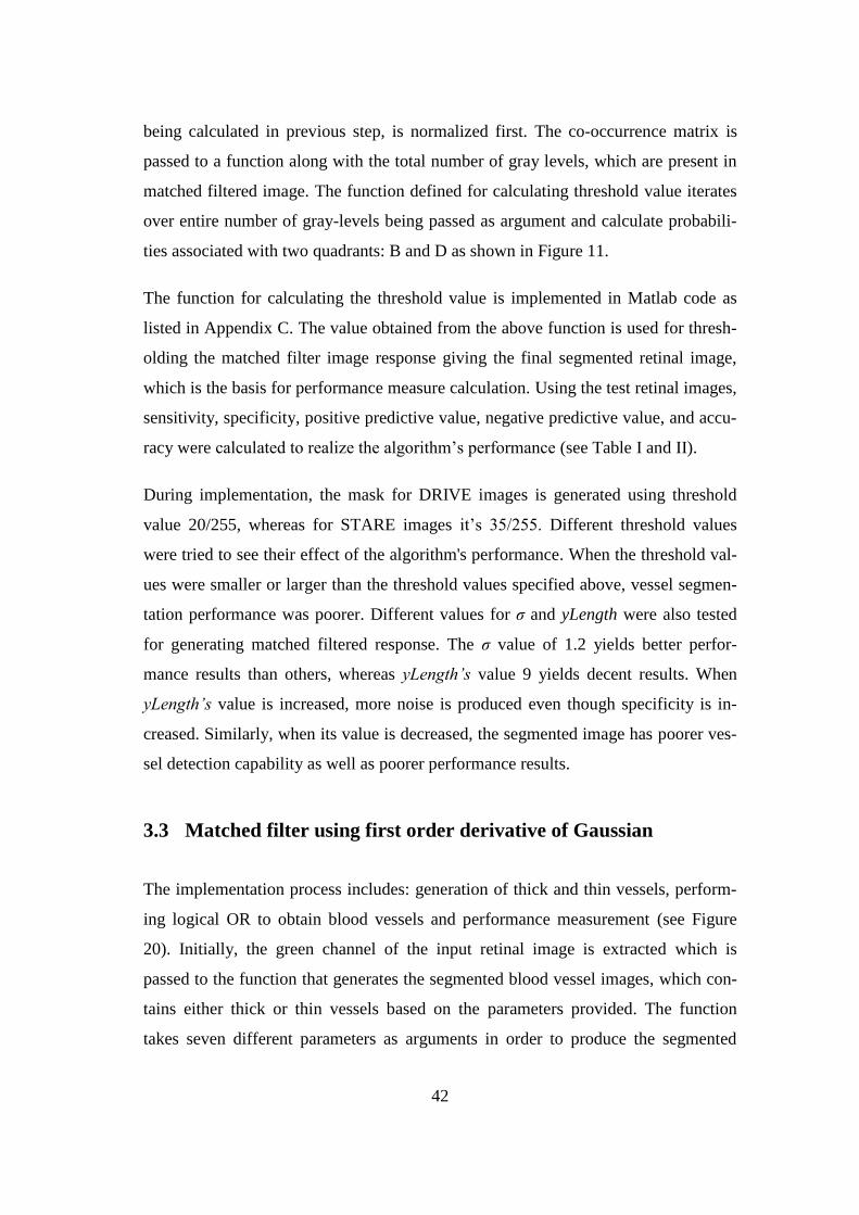
42

being calculated in previous step, is normalized first. The co-occurrence matrix is

passed to a function along with the total number of gray levels, which are present in

matched filtered image. The function defined for calculating threshold value iterates

over entire number of gray-levels being passed as argument and calculate probabili-

ties associated with two quadrants: B and D as shown in Figure 11.

The function for calculating the threshold value is implemented in Matlab code as

listed in Appendix C. The value obtained from the above function is used for thresh-

olding the matched filter image response giving the final segmented retinal image,

which is the basis for performance measure calculation. Using the test retinal images,

sensitivity, specificity, positive predictive value, negative predictive value, and accu-

racy were calculated to realize the algorithm’s performance (see Table I and II).

During implementation, the mask for DRIVE images is generated using threshold

value 20/255, whereas for STARE images it’s 35/255. Different threshold values

were tried to see their effect of the algorithm's performance. When the threshold val-

ues were smaller or larger than the threshold values specified above, vessel segmen-

tation performance was poorer. Different values for σ and yLength were also tested

for generating matched filtered response. The σ value of 1.2 yields better perfor-

mance results than others, whereas yLength’s value 9 yields decent results. When

yLength’s value is increased, more noise is produced even though specificity is in-

creased. Similarly, when its value is decreased, the segmented image has poorer ves-

sel detection capability as well as poorer performance results.

3.3 Matched filter using first order derivative of Gaussian

The implementation process includes: generation of thick and thin vessels, perform-

ing logical OR to obtain blood vessels and performance measurement (see Figure

20). Initially, the green channel of the input retinal image is extracted which is

passed to the function that generates the segmented blood vessel images, which con-

tains either thick or thin vessels based on the parameters provided. The function

takes seven different parameters as arguments in order to produce the segmented

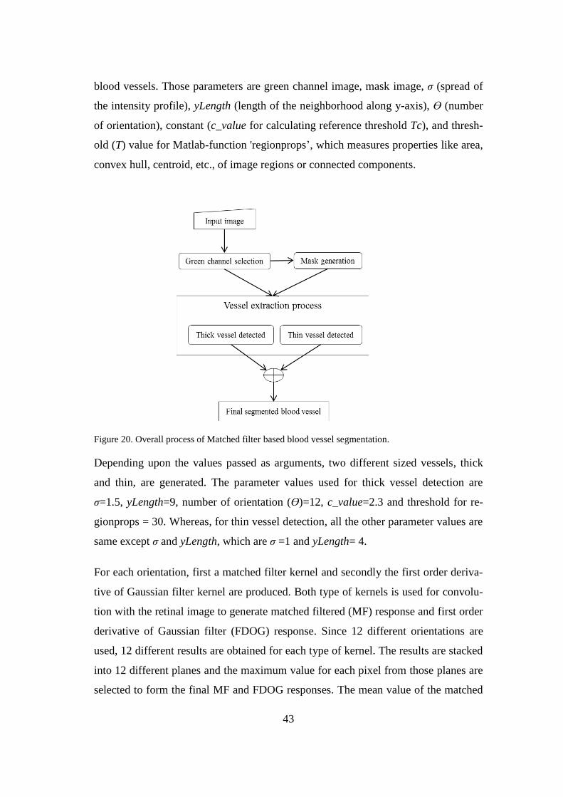
43

blood vessels. Those parameters are green channel image, mask image, σ (spread of

the intensity profile), yLength (length of the neighborhood along y-axis), ϴ (number

of orientation), constant (c_value for calculating reference threshold Tc), and thresh-

old (T) value for Matlab-function 'regionprops’, which measures properties like area,

convex hull, centroid, etc., of image regions or connected components.

Figure 20. Overall process of Matched filter based blood vessel segmentation.

Depending upon the values passed as arguments, two different sized vessels, thick

and thin, are generated. The parameter values used for thick vessel detection are

σ=1.5, yLength=9, number of orientation (ϴ)=12, c_value=2.3 and threshold for re-

gionprops = 30. Whereas, for thin vessel detection, all the other parameter values are

same except σ and yLength, which are σ =1 and yLength= 4.

For each orientation, first a matched filter kernel and secondly the first order deriva-

tive of Gaussian filter kernel are produced. Both type of kernels is used for convolu-

tion with the retinal image to generate matched filtered (MF) response and first order

derivative of Gaussian filter (FDOG) response. Since 12 different orientations are

used, 12 different results are obtained for each type of kernel. The results are stacked

into 12 different planes and the maximum value for each pixel from those planes are

selected to form the final MF and FDOG responses. The mean value of the matched

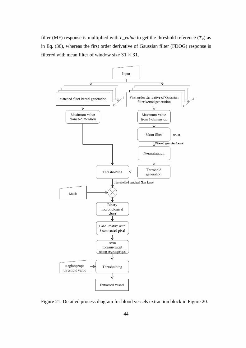
44

filter (MF) response is multiplied with c_value to get the threshold reference (𝑇𝑐) as

in Eq. (36), whereas the first order derivative of Gaussian filter (FDOG) response is

filtered with mean filter of window size 31 × 31.

Figure 21. Detailed process diagram for blood vessels extraction block in Figure 20.

45

The normalized FDOG response and threshold reference (𝑇𝑐) are used to generate the

actual threshold value (T) as in Eq. (35). The threshold value (T) is used for thresh-

olding the matched filter response to detect the blood vessels from a retinal image.

The overall process for extracting blood vessels is illustrated in Figure 21.

The extracted blood vessels in Figure 21 are passed to the post processing block in

order to obtain the final segmented image. During this process, the image is pro-

cessed using morphological closing with structuring element square (3 × 3 pixels)

followed by morphological closing on the binary image. The result is further pro-

cessed by labeling the connected components with a connectivity size of 8 pixels,

and by calculating the ‘area’ property of the image region, which specifies the actual

number of pixels in the region. Finally, the threshold value for regionprops (which

measures properties of image regions) is used for thresholding the ‘area’ property to

get the processed image. If the region’s pixel count is greater than the threshold val-

ue, then it is labeled as a vessel.

The above processes were applied separately, with different parameters, for detecting

thick and thin vessels. The obtained images were combined using logical OR opera-

tion to generate the final segmented blood vessels. Along with the segmented ves-

sels, the performance measures of the algorithm were determined by calculating the

accuracy, true positive rate (TPR) and false positive rate (FPR). TPR and FPR are

equivalent to sensitivity (Se) and specificity (Sp) as mentioned in Table I. The matlab

code for calculating performance measure is listed in Appendix D.

During implementation, the application is divided into three functional blocks; one

for generating matched and Gaussian filter kernels, another for detecting blood ves-

sels and third for measuring performance. The varying parameters are passed to the

function, which detects blood vessels, in order to generate thick and thin vessels in-

dependently. Only the values for sigma (σ), yLength (L), and constant (c) are varied,

while other parameters are unchanged while detecting thick and thin vessels for par-

ticular retinal image. The base values for thick vessels detection are σ =1.5, L=9, and

c=2.3 and for thin one are σ=1, L=4 and c=2.3. Changing the value of c affects the

TPR and FPR but there is no significant difference in accuracy. That is, increasing c

46

value over 2.3 reduces TPR and FPR, while decreasing don’t have adverse effect.

And, small increase or decrease in σ and L value for thick and thin vessels detection,

slightly reduces the performance measures.

47

4 Results

The implemented applications were tested using retinal images from publically

available databases: DRIVE and STARE; and the results were compared against the

corresponding ground truth images to calculate the performance measures of the al-

gorithms. The algorithms for supervised and unsupervised methods of vessel seg-

mentation were evaluated in terms of sensitivity (Se), specificity (Sp), positive pre-

dictive value (Ppv), negative predictive value (Npv), and accuracy (Acc) [8]. The

matched filter algorithm was evaluated in terms of accuracy (Acc), true positive

rate(TPR) and false positive rate(FPR) [20]. The formulas used for calculating these

performance measures are listed in Tables I and II.

The computing system used for running all the applications was a PC with Intel core

i5, 2.6 GHz CPU with 4GB RAM and 1GB of dedicated GPU.

A. Supervised method using gray-level and moment invariant based features with

Neural network

The results obtained for the supervised method of vessel segmentation using gray-

level and moment invariants-based features are listed in Table III and IV.

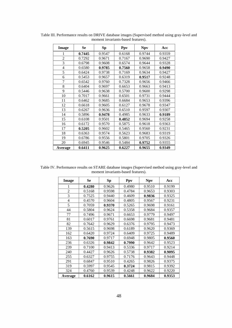
48

Table III. Performance results on DRIVE database images (Supervised method using gray-level and

moment invariants-based features).

Image Se Sp Ppv Npv Acc

1 0.7445 0.9547 0.6168 0.9744 0.9359

2 0.7292 0.9671 0.7167 0.9690 0.9427

3 0.6798 0.9608 0.6574 0.9644 0.9328

4 0.6580 0.9785 0.7560 0.9658 0.9490

5 0.6424 0.9738 0.7169 0.9634 0.9427

6 0.5453 0.9657 0.6319 0.9517 0.9248

7 0.6542 0.9760 0.7328 0.9656 0.9466

8 0.6404 0.9697 0.6653 0.9663 0.9413

9 0.5446 0.9638 0.5700 0.9600 0.9298

10 0.7017 0.9661 0.6501 0.9731 0.9444

11 0.6462 0.9685 0.6684 0.9653 0.9396

12 0.6618 0.9605 0.6127 0.9678 0.9347

13 0.6267 0.9636 0.6510 0.9597 0.9307

14 0.5896 0.9478 0.4985 0.9633 0.9189

15 0.6108 0.9501 0.4852 0.9694 0.9258

16 0.6172 0.9570 0.5875 0.9618 0.9363

17 0.5205 0.9602 0.5465 0.9560 0.9231

18 0.6363 0.9574 0.5623 0.9683 0.9319

19 0.6786 0.9556 0.5801 0.9705 0.9326

20 0.6945 0.9546 0.5484 0.9752 0.9355

Average 0.6411 0.9625 0.6227 0.9655 0.9349

Table IV. Performance results on STARE database images (Supervised method using gray-level and

moment invariants-based features).

Image Se Sp Ppv Npv Acc

1 0.4280 0.9626 0.4980 0.9510 0.9199

2 0.5168 0.9598 0.4784 0.9653 0.9303

3 0.7525 0.9440 0.4609 0.9836 0.9325

4 0.4570 0.9604 0.4805 0.9567 0.9231

5 0.7059 0.9370 0.5265 0.9698 0.9161

44 0.5804 0.9624 0.5358 0.9684 0.9357

77 0.7496 0.9671 0.6653 0.9779 0.9497

81 0.6017 0.9761 0.6698 0.9681 0.9481

82 0.7642 0.9629 0.6376 0.9795 0.9473

139 0.5615 0.9698 0.6189 0.9620 0.9369

162 0.6420 0.9724 0.6409 0.9725 0.9489

163 0.7690 0.9717 0.6948 0.9805 0.9560

236 0.6326 0.9842 0.7990 0.9642 0.9523

239 0.7100 0.9413 0.5336 0.9717 0.9214

240 0.4427 0.9626 0.5738 0.9382 0.9095

255 0.6327 0.9755 0.7176 0.9643 0.9448

291 0.6847 0.9510 0.4265 0.9826 0.9375

319 0.5997 0.9545 0.3724 0.9815 0.9392

324 0.4760 0.9539 0.4248 0.9622 0.9220

Average 0.6162 0.9615 0.5661 0.9684 0.9353

49

For training the neural network, image 27 from the training set of DRIVE images

was used. Whereas for the STARE database, image 255 was used. The original au-

thors' implementation of the algorithm used one input, three hidden layers each with

15 nodes and one output layer for both databases. In this thesis, one input, one hid-

den layer and one output layer were used. A neural network using the authors' origi-

nal configuration was also implemented, but the results were found to be poorer than

with the new configuration. New configurations were chosen for both databases with

the varying number of nodes in the hidden layer. For the DRIVE images, training is

done with 20 nodes in a hidden layer, while for the STARE images, training was

done with 15 nodes. The training took around 25 minutes while simulation or testing

required only 5 seconds to execute. For the DRIVE database, smaller amounts of

nodes (e.g., 10 and 15) gave poorer classification accuracies and sensitivities than 20

nodes, which gave optimal performance results. Similarly, for STARE images, hid-

den layer with 10 and 20 nodes were tested but the optimal results were obtained

using 15 nodes in hidden layer.

The performance results shown in Tables III and IV were obtained by applying the

same threshold value Th for all the images in the same database (for DRIVE, 0.53

and for STARE, 0.43 were used). These threshold values are different than the values

used by the original author, which were 0.63 and 0.91 for DRIVE and STARE imag-

es, respectively. When comparing with the original author’s results, the implement-

ed algorithm gives nearly same accuracy, specificity and negative predictive value

(see Table V). The sensitivity and positive predictive value are smaller than original

author’s result. The implemented algorithm has slightly lower capability to detect

thin vessels, which might be the reason for obtaining smaller values for Se and Ppv.

The use of only one hidden layer rather than three layers in the neural network might

explain the results obtained.

Table V. Comparison of performance results with original author (Supervised method using gray-level

and moment invariants-based features).

Results Se Sp Ppv Npv Acc

Original author 0.7005 0.9810 0.8330 0.9620 0.9489

Our application 0.6286 0.9620 0.5944 0.9669 0.9351

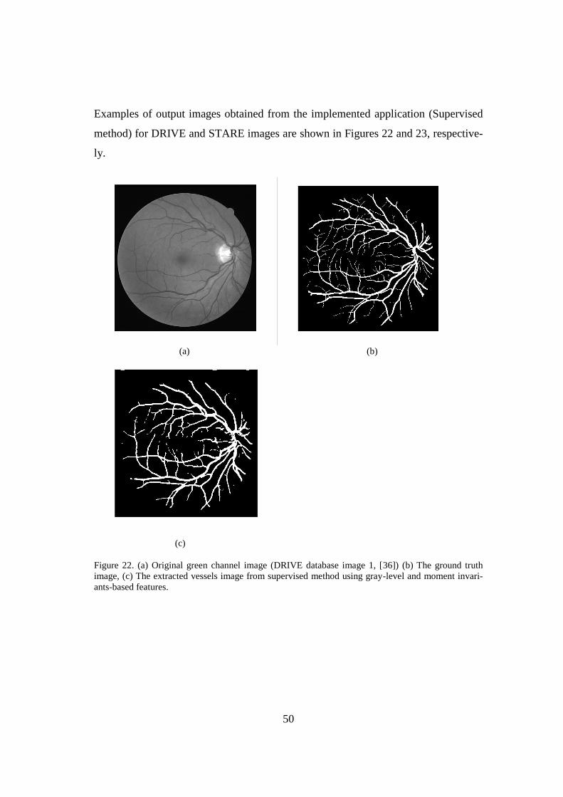
50

Examples of output images obtained from the implemented application (Supervised

method) for DRIVE and STARE images are shown in Figures 22 and 23, respective-

ly.

(a) (b)

(c)

Figure 22. (a) Original green channel image (DRIVE database image 1, [36]) (b) The ground truth

image, (c) The extracted vessels image from supervised method using gray-level and moment invari-

ants-based features.

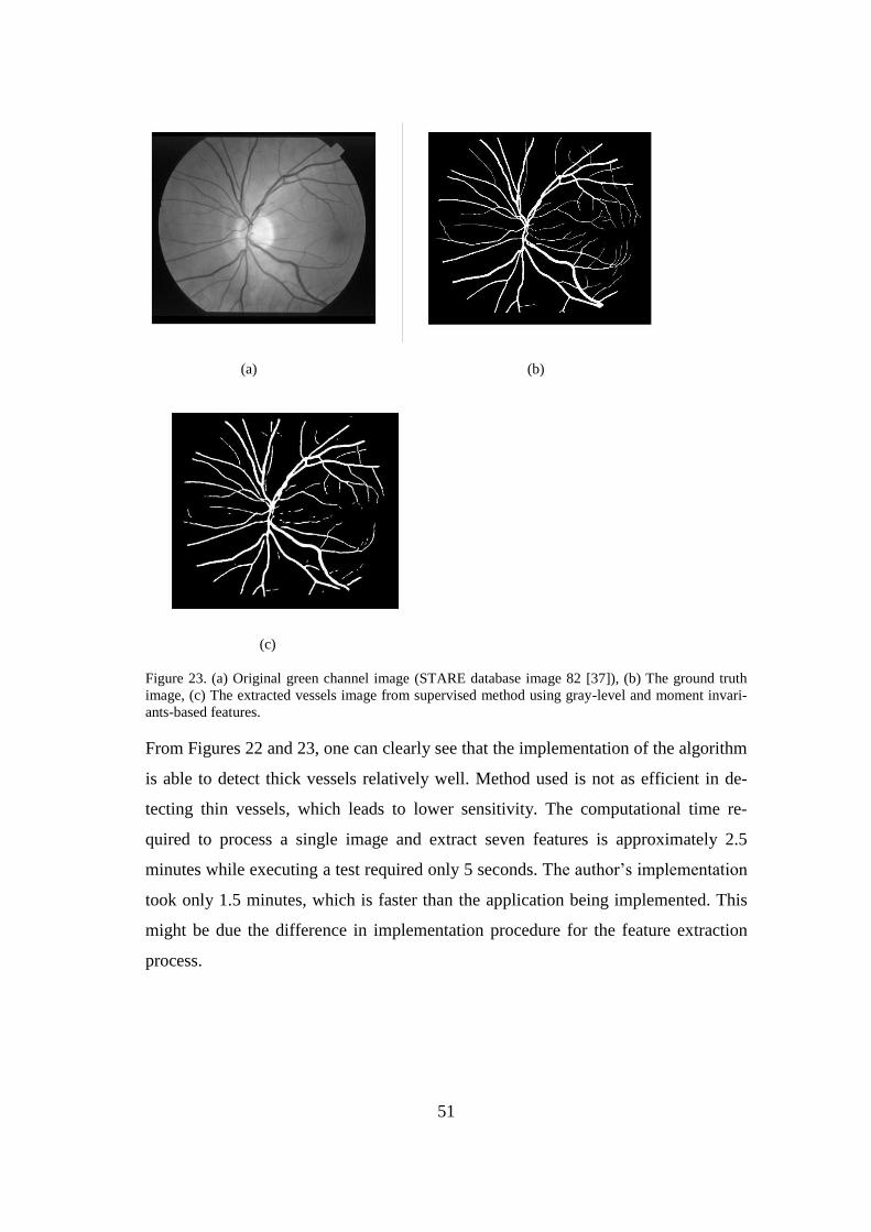
51

(a) (b)

(c)

Figure 23. (a) Original green channel image (STARE database image 82 [37]), (b) The ground truth

image, (c) The extracted vessels image from supervised method using gray-level and moment invari-

ants-based features.

From Figures 22 and 23, one can clearly see that the implementation of the algorithm

is able to detect thick vessels relatively well. Method used is not as efficient in de-

tecting thin vessels, which leads to lower sensitivity. The computational time re-

quired to process a single image and extract seven features is approximately 2.5

minutes while executing a test required only 5 seconds. The author’s implementation

took only 1.5 minutes, which is faster than the application being implemented. This

might be due the difference in implementation procedure for the feature extraction

process.

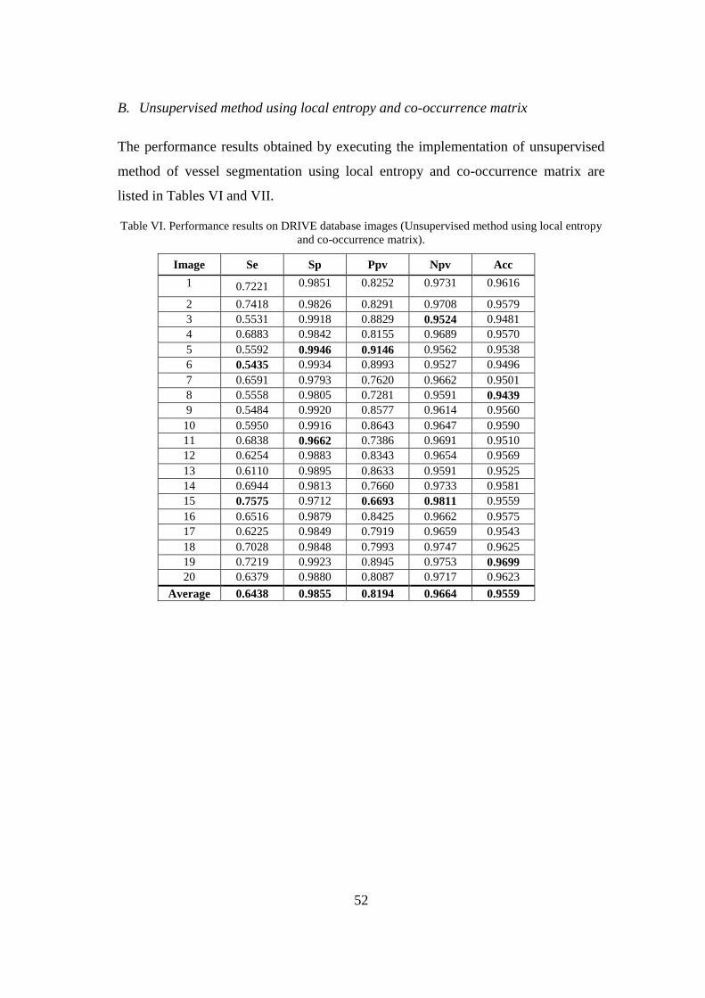
52

B. Unsupervised method using local entropy and co-occurrence matrix

The performance results obtained by executing the implementation of unsupervised

method of vessel segmentation using local entropy and co-occurrence matrix are

listed in Tables VI and VII.

Table VI. Performance results on DRIVE database images (Unsupervised method using local entropy

and co-occurrence matrix).

Image Se Sp Ppv Npv Acc

1 0.7221 0.9851 0.8252 0.9731 0.9616

2 0.7418 0.9826 0.8291 0.9708 0.9579

3 0.5531 0.9918 0.8829 0.9524 0.9481

4 0.6883 0.9842 0.8155 0.9689 0.9570

5 0.5592 0.9946 0.9146 0.9562 0.9538

6 0.5435 0.9934 0.8993 0.9527 0.9496

7 0.6591 0.9793 0.7620 0.9662 0.9501

8 0.5558 0.9805 0.7281 0.9591 0.9439

9 0.5484 0.9920 0.8577 0.9614 0.9560

10 0.5950 0.9916 0.8643 0.9647 0.9590

11 0.6838 0.9662 0.7386 0.9691 0.9510

12 0.6254 0.9883 0.8343 0.9654 0.9569

13 0.6110 0.9895 0.8633 0.9591 0.9525

14 0.6944 0.9813 0.7660 0.9733 0.9581

15 0.7575 0.9712 0.6693 0.9811 0.9559

16 0.6516 0.9879 0.8425 0.9662 0.9575

17 0.6225 0.9849 0.7919 0.9659 0.9543

18 0.7028 0.9848 0.7993 0.9747 0.9625

19 0.7219 0.9923 0.8945 0.9753 0.9699

20 0.6379 0.9880 0.8087 0.9717 0.9623

Average 0.6438 0.9855 0.8194 0.9664 0.9559

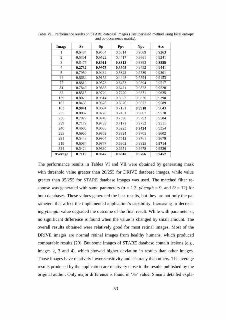
53

Table VII. Performance results on STARE database images (Unsupervised method using local entropy

and co-occurrence matrix).

Image Se Sp Ppv Npv Acc

1 0.6484 0.9504 0.5314 0.9689 0.9263

2 0.5301 0.9522 0.4417 0.9661 0.9241

3 0.8477 0.8911 0.3313 0.9892 0.8885

4 0.2782 0.9973 0.8908 0.9452 0.9441

5 0.7950 0.9434 0.5822 0.9789 0.9301

44 0.8684 0.9188 0.4448 0.9894 0.9153

77 0.8819 0.9578 0.6453 0.9894 0.9517

81 0.7849 0.9655 0.6471 0.9823 0.9520

82 0.8515 0.9720 0.7220 0.9871 0.9625

139 0.8079 0.9514 0.5922 0.9826 0.9398

162 0.8433 0.9678 0.6676 0.9877 0.9589

163 0.9041 0.9694 0.7121 0.9918 0.9643

235 0.8037 0.9728 0.7431 0.9807 0.9578

236 0.7929 0.9749 0.7590 0.9793 0.9584

239 0.7179 0.9733 0.7172 0.9732 0.9511

240 0.4685 0.9885 0.8223 0.9424 0.9354

255 0.6950 0.9862 0.8324 0.9705 0.9602

291 0.5448 0.9904 0.7512 0.9761 0.9679

319 0.6084 0.9877 0.6902 0.9825 0.9714

324 0.5424 0.9830 0.6951 0.9678 0.9536

Average 0.7110 0.9647 0.6610 0.9766 0.9457

The performance results in Tables VI and VII were obtained by generating mask

with threshold value greater than 20/255 for DRIVE database images, while value

greater than 35/255 for STARE database images was used. The matched filter re-

sponse was generated with same parameters (σ = 1.2, yLength = 9, and ϴ = 12) for

both databases. These values generated the best results, but they are not only the pa-

rameters that affect the implemented application’s capability. Increasing or decreas-

ing yLength value degraded the outcome of the final result. While with parameter σ,

no significant difference is found when the value is changed by small amount. The

overall results obtained were relatively good for most retinal images. Most of the

DRIVE images are normal retinal images from healthy humans, which produced

comparable results [20]. But some images of STARE database contain lesions (e.g.,

images 2, 3 and 4), which showed higher deviation in results than other images.

Those images have relatively lower sensitivity and accuracy than others. The average

results produced by the application are relatively close to the results published by the

original author. Only major difference is found in ‘Se’ value. Since a detailed expla-

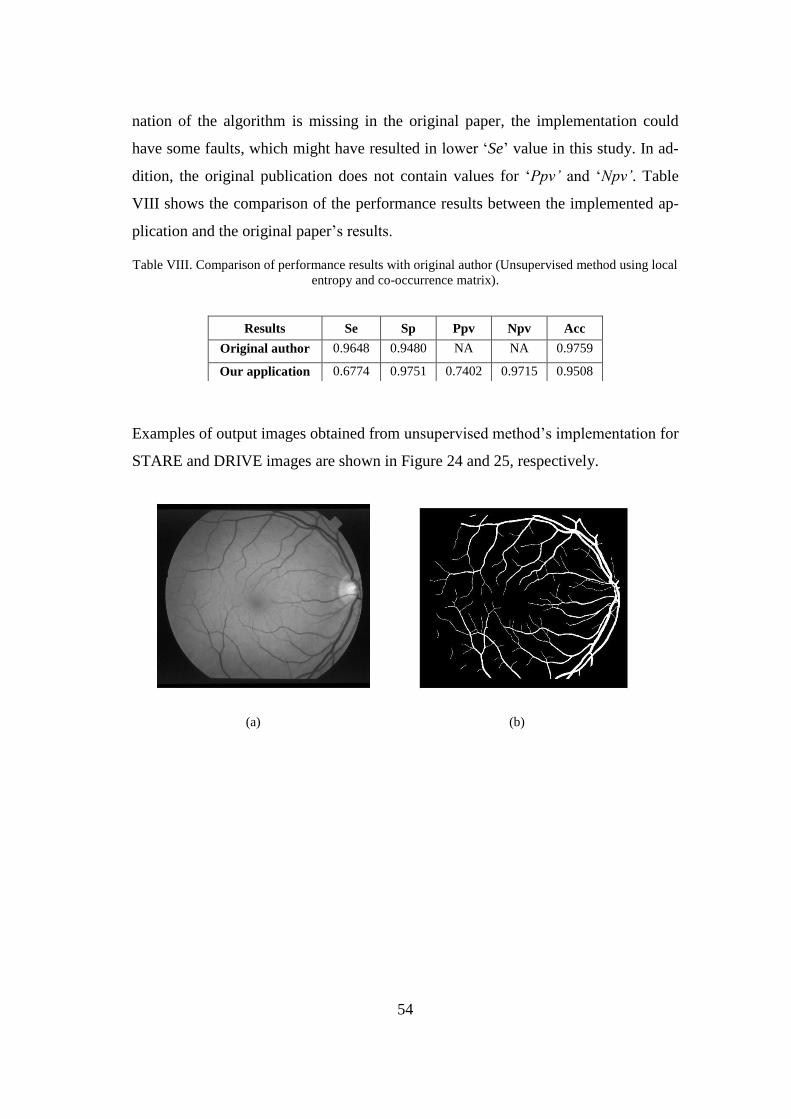
54

nation of the algorithm is missing in the original paper, the implementation could

have some faults, which might have resulted in lower ‘Se’ value in this study. In ad-

dition, the original publication does not contain values for ‘Ppv’ and ‘Npv’. Table

VIII shows the comparison of the performance results between the implemented ap-

plication and the original paper’s results.

Table VIII. Comparison of performance results with original author (Unsupervised method using local

entropy and co-occurrence matrix).

Examples of output images obtained from unsupervised method’s implementation for

STARE and DRIVE images are shown in Figure 24 and 25, respectively.

(a) (b)

Results Se Sp Ppv Npv Acc

Original author 0.9648 0.9480 NA NA 0.9759

Our application 0.6774 0.9751 0.7402 0.9715 0.9508

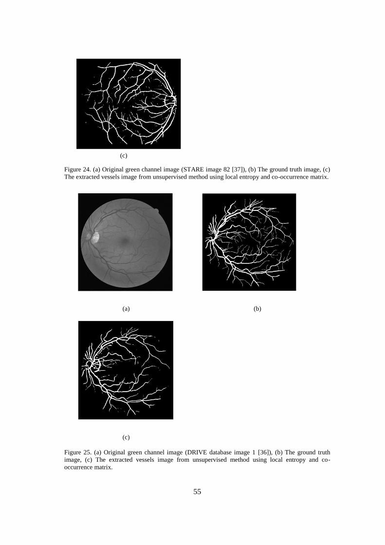
55

Figure 24. (a) Original green channel image (STARE image 82 [37]), (b) The ground truth image, (c)

The extracted vessels image from unsupervised method using local entropy and co-occurrence matrix.

(a) (b)

(c)

Figure 25. (a) Original green channel image (DRIVE database image 1 [36]), (b) The ground truth

image, (c) The extracted vessels image from unsupervised method using local entropy and co-

occurrence matrix.

(c)

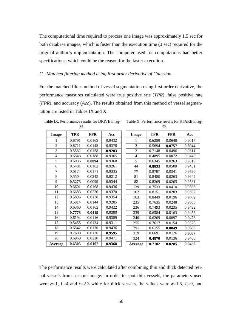
56

The computational time required to process one image was approximately 1.5 sec for

both database images, which is faster than the execution time (3 sec) required for the

original author’s implementation. The computer used for computations had better

specifications, which could be the reason for the faster execution.

C. Matched filtering method using first order derivative of Gaussian

For the matched filter method of vessel segmentation using first order derivative, the

performance measures calculated were true positive rate (TPR), false positive rate

(FPR), and accuracy (Acc). The results obtained from this method of vessel segmen-

tation are listed in Tables IX and X.

Table IX. Performance results for DRIVE imag-

es.

Image TPR FPR Acc

1 0.6791 0.0163 0.9432

2 0.6711 0.0145 0.9378

3 0.5532 0.0158 0.9203

4 0.6543 0.0188 0.9365

5 0.6035 0.0094 0.9368

6 0.5481 0.0102 0.9261

7 0.6174 0.0171 0.9335

8 0.5504 0.0245 0.9212

9 0.5275 0.0099 0.9344

10 0.6601 0.0168 0.9436

11 0.6683 0.0220 0.9370

12 0.5896 0.0138 0.9354

13 0.5914 0.0144 0.9285

14 0.6360 0.0162 0.9422

15 0.7778 0.0419 0.9390

16 0.6194 0.0116 0.9389

17 0.5455 0.0134 0.9311

18 0.6542 0.0176 0.9436

19 0.7690 0.0136 0.9595

20 0.6960 0.0220 0.9471

Average 0.6305 0.0167 0.9368

Table X. Performance results for STARE imag-

es.

Image TPR FPR Acc

1 0.6289 0.0648 0.9017

2 0.5694 0.0757 0.8944

3 0.7148 0.0496 0.9311

4 0.4895 0.0072 0.9440

5 0.6345 0.0263 0.9315

44 0.8833 0.0509 0.9451

77 0.8797 0.0341 0.9590

81 0.8450 0.0263 0.9642

82 0.8209 0.0265 0.9581

139 0.7533 0.0410 0.9366

162 0.8151 0.0283 0.9562

163 0.8449 0.0196 0.9662

235 0.7635 0.0248 0.9503

236 0.7493 0.0235 0.9492

239 0.6584 0.0163 0.9453

240 0.6209 0.0097 0.9473

255 0.7617 0.0154 0.9578

291 0.6155 0.0049 0.9683

319 0.6691 0.0126 0.9687

324 0.4870 0.0136 0.9400

Average 0.7102 0.0285 0.9456

The performance results were calculated after combining thin and thick detected reti-

nal vessels from a same image. In order to spot thin vessels, the parameters used

were σ=1, L=4 and c=2.3 while for thick vessels, the values were σ=1.5, L=9, and

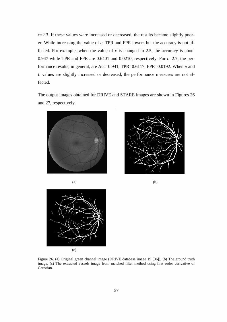
57

c=2.3. If these values were increased or decreased, the results became slightly poor-

er. While increasing the value of c, TPR and FPR lowers but the accuracy is not af-

fected. For example; when the value of c is changed to 2.5, the accuracy is about

0.947 while TPR and FPR are 0.6401 and 0.0210, respectively. For c=2.7, the per-

formance results, in general, are Acc=0.941, TPR=0.6117, FPR=0.0192. When σ and

L values are slightly increased or decreased, the performance measures are not af-

fected.

The output images obtained for DRIVE and STARE images are shown in Figures 26

and 27, respectively.

(a) (b)

Figure 26. (a) Original green channel image (DRIVE database image 19 [36]), (b) The ground truth

image, (c) The extracted vessels image from matched filter method using first order derivative of

Gaussian.

(c)

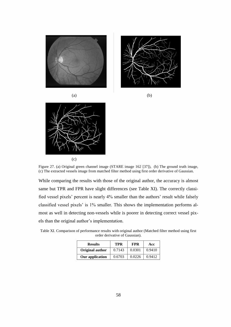
58

(a) (b)

Figure 27. (a) Original green channel image (STARE image 162 [37]), (b) The ground truth image,

(c) The extracted vessels image from matched filter method using first order derivative of Gaussian.

While comparing the results with those of the original author, the accuracy is almost

same but TPR and FPR have slight differences (see Table XI). The correctly classi-

fied vessel pixels’ percent is nearly 4% smaller than the authors’ result while falsely

classified vessel pixels’ is 1% smaller. This shows the implementation performs al-

most as well in detecting non-vessels while is poorer in detecting correct vessel pix-

els than the original author’s implementation.

Table XI. Comparison of performance results with original author (Matched filter method using first

order derivative of Gaussian).

Results TPR FPR Acc

Original author 0.7143 0.0301 0.9410

Our application 0.6703 0.0226 0.9412

(c)

59

The computational time required was about 1.5 sec to process one image for both

database images, which was faster than the execution time (10 sec) required for the

original author’s implementation.

Some vessel segmented images obtained from three different implemented algo-

rithms are listed in Appendix A.

60

5 Conclusion

In this thesis, the literatures regarding different methods for retinal blood vessel seg-

mentation were studied and three different state-of-the-art methods were implement-

ed [8, 12, 20]. Based on the study of literature and selection of three different meth-

ods, the issues addressed in this thesis are: 1) How accurate are the selected blood

vessel segmentation methods in extracting blood vessels from fundus images, and 2)

Are results from automated blood vessel extraction systems trustworthy compared to

manual segmentations done by experts.

There are different types of blood vessel segmentation algorithms available which

are mentioned in chapter 2. To test and evaluate the algorithms, fundus images are

needed. Hence, the publicly available image databases STARE and DRIVE play an

important role for evaluating and measuring the performance of algorithms, which

are presented in chapter 2. These databases contain fundus images for training and

testing algorithms including the corresponding ground truth images. Due to its avail-

ability for general public, the study and performance estimation of vessel segmenta-

tion algorithms has become easy. In this thesis, the three state-of-the-art methods [8,

12, 20] from three different categories (i.e. supervised, unsupervised, and match fil-

tering methods) were selected based on their good performance results as published

in the literature. The individual methods were studied in detail and described in chap-

ter 2.

Among the three state-of-the-art methods, the literature related to the supervised

method [8] and matched filtering based method [12] are well documented, which

made the implementation process easier. Whereas the unsupervised method [20] is

relatively poorly documented, so other similar kind of literature [69, 70] was taken

into consideration for studying and implementing the algorithm.

For supervised method based algorithm, the performance results are better for

DRIVE database images than for STARE (see Table III and IV). When the overall

results are compared with the state-of-the-art method's results, the algorithm has

61

lower performance results which are illustrated in Table V. The possible reasons

could be due to difference in neural network design and selection of different thresh-

old values than used in the original publication. When NN was trained with three

hidden layers, each having 15 neurons as in the original literature, the results were

relatively poor. So a new NN was designed with one hidden layer containing 15 neu-

rons, which produced slightly better performance results. According to the original

literature, the threshold values of 0.63 and 0.91 were used for DRIVE and STARE

database images, respectively. The algorithm implemented in this thesis used values

of 0.53 and 0.43 for DRIVE and STARE, respectively, as those threshold values

generated the optimal results.

For unsupervised method based algorithm, the sensitivity values for STARE database

images are better than for DRIVE, while positive predictive values (Ppv) for DRIVE

database images are better than for STARE. Other performance measures are nearly

the same for both image databases (see Table VI and VII). The overall results ob-

tained from algorithm are lower than the ones in the original publication which are

shown in Table VIII. The accuracy and specificity are nearly the same, but the im-

plemented algorithm's sensitivity is relatively low compared to the original result.

Since the literature is hard to understand due to its poor documentation, the algo-

rithm's details could have been misunderstood, for example, in the cases of GLCM

calculation and JRE thresholding. This could be the main reason for obtaining lower

results from the algorithm. The literature lacks explanation about parameters' values

used for evaluating the algorithm and also the results; positive predictive value (Ppv)

and negative predictive value (Npv) (see Table VIII). Moreover, the matched filter

based algorithm’s results are nearly the same with slightly better true positive rate

(TPR) for DRIVE database images. When the algorithm’s results are compared to the

state-of-the-art method's results, the implemented algorithm has lower TPR while

other measures are in close approximation, which are shown in Table XI.

After analyzing the results of three different algorithms, it is found that the perfor-

mance results of state-of-the-art methods are better than the results of the implement-

ed algorithms. Furthermore, the images with high level of lesions have poorer per-

62

formance results than the normal retinal images. Although the accuracy of all three

methods is nearly the same when compared with the corresponding state-of-the-art

methods, the distinguishing characteristic (i.e., lower sensitivity value) is found in

the all implemented algorithms. This has affected the determination of the amount of

correctly classified vessel pixels. Hence, the true vessel detection rate is lower. How-

ever, the algorithms have high accuracy (i.e., more than 93 percent for all methods),

which could be the key factor for accepting the algorithms to be used for the extrac-

tion of blood vessels.

The algorithms have capability of detecting vessels and background from fundus

images but only to a certain extent. As the manual segmentation of blood vessels is

hard and time consuming, it would be better to use a fast, automated system which

could detect higher amount of blood vessels. Besides saving time, it could decrease

the number of experts required and increase the ability to segment large numbers of

fundus images in a short period of time. Since the currently implemented algorithms

have relatively low correctly classified vessel rates, they are not feasible for imple-

mentation into automatized system. Although the accuracy rate of algorithms is rea-

sonable, improvement in the true vessel and background detection should be done.

Hence, the automated vessel detection system is not fully trustworthy with the results

being achieved.

There are few areas for improving the algorithms’ performance. The algorithms were

evaluated using only DRIVE and STARE image databases, which might be not

enough for analyzing the algorithms to full extent. So, for the evaluation of algo-

rithms, other available image databases could be included. In addition, the noise in

fundus image usually lowers the overall results, if it is not handled properly. Hence,

other preprocessing and post-processing strategies could be included along with the

existing ones in order to improve the overall performance results. The study of these

subjects is considered to be important for the future research.

63

References

[1] Soares J.V., Leandro J.J., Cesar R.M., Jelinek H.F., Cree M.J., (2006): Retinal

vessel segmentation using the 2-D Gabor wavelet and supervised classification.

IEEE Transaction of Medical Imaging, vol.25, pp.1214–1222.

[2] Fathi A., Naghsh-Nilchi A.R. (2012): Automatic wavelet-based retinal blood

vessels segmentation and vessel diameter estimation. Biomedical Signal Pro-

cessing and Control, vol.8(1), pp.71-80.

[3] Fang B., Hsu W., Lee M.U., (2003): On the Detection of Retinal Vessels in

Fundus Images. http://hdl.handle.net/1721.1/3675 (04.05.2016)

[4] You X., Peng Q., Yuan Y., Cheung Y., Lei J. (2011): Segmentation of retinal

blood vessels using the radial projection and semi-supervised approach. Pattern

Recognition, vol.44, pp.2314-2324.

[5] Wasan B., Cerutti A., Ford S., Marsh R., (1995): Vascular network changes in

the retina with age and hypertension. Journal of Hypertension, vol.13(12),

pp.1724-1728.

[6] Sussman E.J., Tsiaras W.G., Soper K.A., (1982): Diagnosis of diabetic eye dis-

ease. The Journal of the American Medical Association, vol.247(23), pp.3231-

3234.

[7] Nguyen U.T., Bhuiyan A., Park L.A., Ramamohanarao K., (2013): An effective

retinal blood vessel segmentation method using multi-scale line detection. Pat-

tern Recognition, vol.46, pp.703-715.

[8] Diego M., Arturo A., Manuel E., and Jose M. (2011): A new supervised method

for blood vessel segmentation in retinal images by using gray-level and moment

invariants-based features. IEEE Transactions on Medical Imaging, vol.30(1),

pp.146-158.

[9] Ricci E., Perfetti R., (2007): Retinal blood vessel segmentation using line opera-

tors and support vector classification. IEEE Transaction of Medical Imaging,

vol.26, pp.1357–1365.

64

[10] Staal J., Abramoff M.D., Niemeijer M., Viergever M.A., Ginneken B., (2004):

Ridge-based vessel segmentation in color images of the retina. IEEE Transac-

tions on Medical Imaging, vol.23, pp.501-509.

[11] Sinthanayothin C., Boyce J., Williamson C.T., (1999): Automated localisation

of the optic disk, fovea, and retinal blood vessels from digital colour fundus im-

ages. The British Journal of Ophthalmology, vol.83(8), pp.902-910.

[12] Villalobos-Castaldi F.M., Felipe-Riveron E.M., Sanchez-Fernandez L.P.,

(2010): A fast, efficient and automated method to extract vessels from fundus

images. Journal of Visualization, vol.13, pp.263-270.

[13] Kande G.B., Subbaiah P.V., Savithri T.S., (2009): Unsupervised fuzzy based

vessel segmentation in pathological digital fundus images. Journal of Medical

Systems, vol.34, pp.849-858.

[14] Rahebi J., Hardalac F., (2014): Retinal Blood Vessel Segmentation with Neural

Network by Using Gray-Level Co-Occurrence Matrix-Based Features. Journal

of Medical Systems, vol.38(8), pp.85-97.

[15] Tolias Y., Panas S., (1998): A fuzzy vessel tracking algorithm for retinal images

based on fuzzy clustering. IEEE Transactions on Medical Imaging, vol.17(2),

pp.263-273.

[16] Al-Rawi M., Qutaishat M., Arrar M. (2006): An improved matched filter for

blood vessel detection of digital retinal images. Computers in Biology and Med-

icine, vol.37, pp.262-267.

[17] Chaudhuri S., Chatterjee S., Katz N., Nelson M., and Goldbaum M. (1989): De-

tection of blood vessels in retinal images using two-dimensional matched filters.

IEEE Transaction on Medical Imaging, vol.8, pp.263–269.

[18] Zolfagharnasab H., Naghsh-Nilchi A.R. (2014): Cauchy based matched filter for

retinal vessels detection. Journal of Medical Signals and Sensors, vol.4(1), pp.

1-9.

[19] Hoover A., Kouznetsova V., Goldbaum M. (2000): Locating blood vessels in

retinal images by piecewise threshold probing of a matched filter response.

IEEE Transaction on Medical Imaging, vol.19(3), pp.203-210.

65

[20] Zhang B., Zhang L., Karray F., (2010): Retinal vessel extraction by matched

filter with first-order derivative of Gaussian. Computers in Biology and Medi-

cine, vol.40, pp.438-445.

[21] Fraz M.M., Remagnino P., Hoppe A., Uyyanonvara B., Rudnicka A., Owen C.,

Barman S. (2012): Blood vessel segmentation methodologies in retinal images –

A survey. Computer Methods and Programs in Biomedicine, vol.108, pp. 407-

433.

[22] Sun K., Chen Z., Jiang S., Wang Y. (2011): Morphological multiscale enhance-

ment, fuzzy filter and watershed for vascular tree extraction in angiogram. Jour-

nal of Medical Systems, vol.35(5), pp.811-824.

[23] Mookiah M.R., Acharya U.R., Chua C.K., Lim C.M., Laude A. (2013): Com-

puter-aided diagnosis of diabetic retinopathy: A review. Computers in Biology

and Medicine, vol.43, pp.2136-2155.

[24] Al-Diri B., Hunter A., Steel D., (2009): An active contour model for segmenting

and measuring retinal vessels. IEEE Transactions on Medical Imaging,

vol.28(9), pp.1488-1497.

[25] Al-Diri B., Hunter A., Steel D. (2009): An active contour model for segmenting

and measuring retinal vessels. IEEE Transactions of Medical Imaging,

vol.38(9), pp.1488-1497.

[26] Lam B.S., Gao Y., Liew A.W. (2010): General retinal vessel segmentation using

regularization based multiconcavity modeling. IEEE Transactions of Medical

Imaging, vol.29, pp.1369-1381.

[27] Sum K.W., Cheung P.Y., (2008): Vessel extraction under non-uniform illumina-

tion: a level set approach. IEEE Transactions on Biomedical Engineering,

vol.55(1), pp.1196-1204.

[28] Osareh A., Shadgar B., (2009): Automatic blood vessel segmentation in color

images of retina. Iranian Journal of Science and Technology, vol.33, pp.191–

206.

[29] Mendonca A.M., Campilho A., (2006): Segmentation of retinal blood vessels by

combining the detection of centerlines and morphological reconstruction. IEEE

Transaction on Medical Imaging, vol.25(9), pp.1200-1213.

66

[30] Taylor H.R., Keeffe J.E., (2001): World blindness: A 21st century perspective.

British Journal of Ophthalmology, vol.85, pp.261-266.

[31] Human eye anatomy: http://www.allaboutvision.com/resources/anatomy.htm

(02.05.2016)

[32] Human eye: http://www.nkcf.org/how-the-human-eye-works/ (02.05.2016)

[33] Human eye diagram: https://nei.nih.gov/health/eyediagram (02.05.2016)

[34] Macula background: http://patient.info/doctor/macular-disorders (03.05.2016)

[35] Montgomery T.: Macula. http://www.tedmontgomery.com/the_eye/macula.html

(03.05.2016)

[36] Research Section, Digital Image for Vessel Extraction (DRIVE) Database.

Utrecht, The Netherlands, Univ. Med. Center Utrecht, Image Sci. Inst.

http://www.isi.uu.nl/Research/Databases/DRIVE/, (05.01.2016)

[37] STARE Project Website. Clemson, SC, Clemson University.

http://www.ces.clemson.edu/~ahoover/stare/, (12.01.2016)

[38] Frangi A.F., Niessen W.J., Vincken K.L., Viergever M.A., William W., Alan C.,

Scott D. (1998): Mulitscale vessel enhancement filtering. Medical Image Com-

puting and Computer-Assisted Interventation, vol.1497, pp.130-137.

[39] Miri M.S., Mahloojifar A. (2011): Retinal image analysis using curvelet trans-

form and multistructure elements morphology by reconstruction. IEEE Transac-

tions on Biomedical Engineering, vol.58, pp.1183-1192.

[40] Sato Y., Araki T., Hanayama M., Naito H., Tamura S. (1998): A viewpoint de-

termination system for stenosis diagnosis and quantification in coronary angio-

graphic image acquisition. IEEE Transactions of Medical Imaging, vol.17(1),

pp.121-137.

[41] Chua L.O., Yang L. (1988): Cellular neural networks. Transaction of Circuits

and Systems, vol.35, pp.1257-1272.

[42] Alonso-Montes C., Vilario D.L., Dudek P., Penedo M.G., (2008): Fast retinal

vessel tree extraction: a pixel parallel approach. International Journal of Circuit

Theory and Applications, vol.36, pp.641-651.

[43] Pattern recognition. http://www.mathworks.com/discovery/pattern-

recognition.html (07.04.2016)

67

[44] Pattern recognition. http://global.britannica.com/technology/pattern-recognition-

computer-science (07.04.2016)

[45] Aksoy S. (2015): Introduction to pattern recognition

http://www.cs.bilkent.edu.tr/~saksoy/courses/cs551/slides/cs551_intro.pdf

(08.04.2016)

[46] Dukart J., (2015): Basic Concepts of Image Classification Algorithms Applied

to Study Neurodegenerative Diseases. Brain Mapping: An Encyclopedic Refer-

ence, vol.3, pp.641-646.

[47] Sathya R., Abraham A., (2013): Comparison of Supervised and Unsupervised

Learning Algorithms for Pattern Classification. International Journal of Ad-

vanced Research in Artificial Intelligence, vol.2(3), pp.34-38.

[48] DongMel C. and Douglas S., (2002): The Effect of Training Strategies on Su-

pervised Classification at Different Spatial Resolutions. Photogrammetric Engi-

neering & Remote Sensing, vol.68(11), pp.1155-1161.

[49] Joao V.S., Jorge J.G., Roberto M.C., Herbert F.J., Michael J.C., (2006): Retinal

Vessel Segmentation Using the 2-D Gabor Wavelet and Supervised Classifica-

tion. IEEE Transaction of Medical Imaging, vol.25, pp.1214-1222.

[50] Elisa R., Renzo P., (2007): Retinal Blood Vessel Segmentation Using Line Op-

erators and Support Vector Classification. IEEE Transaction of Medical Imag-

ing, vol.26, pp.1357-1365.

[51] Ahuja N., RosenFeld A., Haralick R.M., (1980): Neighbor gray levels as fea-

tures in pixel classification. Pattern Recognition, vol.12, pp.251-260.

[52] Rocha L., Velho L., Carvalho P.: Image Moments-Based Structuring and Track-

ing of Objects. Instituto Nacional de Matematica Pura e Aplicada.

http://sibgrapi.sid.inpe.br/col/sid.inpe.br/banon/2002/10.23.11.34/doc/35.pdf

(08.04.2016)

[53] Walter T., Massin P., Erginay A., Ordonez R., Jeulin C., Klein J.C., (2007): Au-

tomatic detection of microaneurysms in color fundus images. Medical Image

Analysis, vol.11, pp.555-566.

[54] Top hat transformation.

http://www.mathworks.com/help/images/ref/imtophat.html (08.04.2016)

68

[55] Kumar G., (2014): A Detailed Review of Feature Extraction in Image Pro-

cessing Systems. Fourth International Conference on Advanced Computing &

Communication Technologies, pp.5-12.

[56] Han Z., Yin Y., Meng X., Yang G., and Yan X., (2014): Blood vessel segmenta-

tion in pathological retinal image. IEEE International Conference on Data Min-

ing Workshop, pp.960-967.

[57] Flusser and Suk. T., (2006): Rotation Moment Invariants for Recognition of

Symmetric Objects. IEEE Transactions on Image Processing, vol.15, pp.3784-

3790.

[58] Dominguez S., (2013): Image analysis by moment invariants using a set of step-

like basis functions. Pattern Recognition Letter, vol.34(16), pp.2065–2070.

[59] Huang Z., & Leng J., (2010): Analysis of Hu’s Moment Invariants on Image

Scaling and Rotation. International Conference on Computer Engineering and

Technology, vol.7, pp.476-480.

[60] Caudill M., (1987): Neural Network Primer: Part I. AI Expert, vol.2(12), pp.46-

52.

[61] Neural network. http://pages.cs.wisc.edu/~bolo/shipyard/neural/local.html.

(10.04.2016).

[62] Huang G.B., Chen Y.Q., Babri H.A., (2000): Classification ability of single hid-

den layer feedforward neural networks. IEEE Transaction on Neural Network,

vol.11, pp.799–801.

[63] Kun J. (2012): Backpropagation algorithm.

https://jeremykun.com/2012/12/09/neural-networks-and-backpropagation/

(11.04.2016).

[64] Soares J.B., Leandro J.G., Cesar R.M., Jelinek H.F., Cree M.J., (2006): Retinal

vessel segmentation using the 2-D Gabor wavelet and supervised classification.

IEEE Transactions on Medical Imaging, vol.25, pp.1214-1222.

[65] You X., Peng Q., Yuan Y., Cheung Y., Lei J., (2011): Segmentation of retinal

blood vessels using the radial projection and semi-supervised approach. Pattern

Recognition, vol.44, pp.2314-2324.

69

[66] Niemeijer M., Staal J.J., Ginneken B., Loog M., Abramoff M.D., (2004): Com-

parative study of retinal vessel segmentation methods on a new publicly availa-

ble database. SPIE Medical Imaging, vol.5370, pp.648-656.

[67] Kohonen T., Simula O., (1996): Engineering Applications of the Self-

Organizing Map. Proceeding of the IEEE, vol.84(10), pp.1354-1384.

[68] Unsupervised learning: http://www.economistinsights.com/technology-

innovation/opinion/%E2%80%9Cunsupervised-learning%E2%80%9D-and-

future-analytics (03.04.2016)

[69] Yang C.W., Ma D.J, Wang C.M., Wen C.H., Le C.S., Chang C., (2000): Com-

puter-aided diagnostic detection system of venous beading in retinal images.

Optical Engineering, vol.39(5), pp.1293-1303.

[70] Chanwinmaluang T., Fan G., (2003): An efficient blood vessel detection algo-

rithm for retinal images using local entropy thresholding. International Sympo-

sium on Circuits and Systems, vol.5, pp.21-24.

[71] Aksoy S., Haralick R.M., (1998): Textural Features for Image Database Retriev-

al. Proceedings of IEEE Workshop on Content-Based Access of Image and Vid-

eo Libraries, pp.45-49.

[72] Haralick R.M., Shanmuga K., Dinstein I., (1973): Textural features for image

classification. IEEE Transaction on System, Man and Cybernetics, vol.3(6), pp.

610-621.

[73] Gebejes A., Huertas R., (2013): Texture Characterization based on Grey-Level

Co-occurrence Matrix. Conference of Informatics and Management Sciences,

pp.375-378.

[74] Simo A., Ves E., (2001): Segmentation of macular fluorescein angiographies: A

statistical approach. Pattern Recognition, vol.34, pp.795-809.

[75] Ng J., Clay S.T., Barman S.A., Fielder A.R., Moseley M.J., Parker K.H., Pater-

son C., (2010): Maximum likelihood estimation of vessel parameters from scale

space analysis. Image and Vision Computing, vol.28(1), pp.55-63.

[76] Salem N.M., Salem S.A., and Nandi A.K., (2007): Segmentation of retinal blood

vessels using a novel clustering algorithm (RACAL) with a partial supervision

strategy. Medical and Biological Engineering and Computing, vol.45, pp.261-

273.

70

[77] Chawimaluang T., Fan G. (2003): An effective blood vessel detection algorithm

for retinal images using local entropy thresholding. Proceeding of the 2003 In-

ternational Symposium on Circuits and Systems, vol.5, pp.21-24.

[78] Gaussian function properties:

https://www.dsprelated.com/freebooks/sasp/Gaussian_Function_Properties.html

(28.04.2016).

[79] Kuijper A., (2010): Scale Space and PDE methods in image analysis and pro-

cessing. Technische Universitat Darmstadt, http://www.gris.informatik.tu-

darmstadt.de/~akuijper/course/TUD11/lecture3.pdf, (29.04.2016).

[80] Cinsdikici M.G., Aydin D., (2009): Detection of blood vessels in ophthalmo-

scope images using MF/ant (matched filter/ant colony) algorithm. Computer

Methods and Programs in Biomedicine, vol.96, pp.85-95.

[81] Yao C., Chen H., (2009): Automated retinal blood vessels segmentation based

on simplified PCNN and fast 2D-Otsu algorithm. Journal of Central South Uni-

versity of Technology, vol.16, pp.640-646.

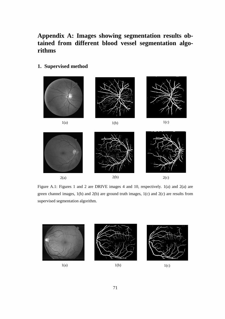
71

Appendix A: Images showing segmentation results ob-

tained from different blood vessel segmentation algo-

rithms

1. Supervised method

Figure A.1: Figures 1 and 2 are DRIVE images 4 and 10, respectively. 1(a) and 2(a) are

green channel images, 1(b) and 2(b) are ground truth images, 1(c) and 2(c) are results from

supervised segmentation algorithm.

1(a) 1(b)

1(c)

2(c)

2(b) 2(a)

1(a)

1(b) 1(c)

1(c)

1(c)

2(c)

1(b)

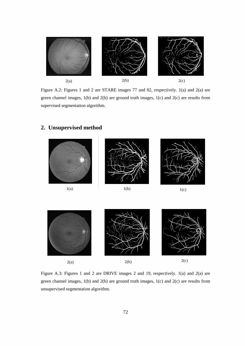
72

Figure A.2: Figures 1 and 2 are STARE images 77 and 82, respectively. 1(a) and 2(a) are

green channel images, 1(b) and 2(b) are ground truth images, 1(c) and 2(c) are results from

supervised segmentation algorithm.

2. Unsupervised method

Figure A.3: Figures 1 and 2 are DRIVE images 2 and 19, respectively. 1(a) and 2(a) are

green channel images, 1(b) and 2(b) are ground truth images, 1(c) and 2(c) are results from

unsupervised segmentation algorithm.

2(a) 2(b) 2(c)

2(a) 2(b) 2(c)

1(a) 1(b) 1(c)

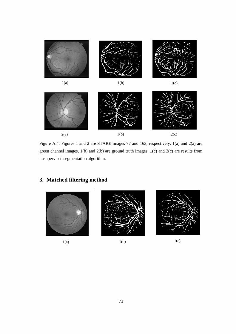
73

Figure A.4: Figures 1 and 2 are STARE images 77 and 163, respectively. 1(a) and 2(a) are

green channel images, 1(b) and 2(b) are ground truth images, 1(c) and 2(c) are results from

unsupervised segmentation algorithm.

3. Matched filtering method

1(a) 1(b)

1(c)

2(c)

2(b) 2(a)

1(a) 1(b)

1(c)

1(c)

1(c)

2(c)

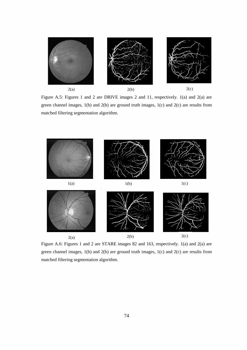
74

Figure A.5: Figures 1 and 2 are DRIVE images 2 and 11, respectively. 1(a) and 2(a) are

green channel images, 1(b) and 2(b) are ground truth images, 1(c) and 2(c) are results from

matched filtering segmentation algorithm.

Figure A.6: Figures 1 and 2 are STARE images 82 and 163, respectively. 1(a) and 2(a) are

green channel images, 1(b) and 2(b) are ground truth images, 1(c) and 2(c) are results from

matched filtering segmentation algorithm.

2(a) 2(b) 2(c)

1(a) 1(b) 1(c)

2(b) 2(a) 2(c)

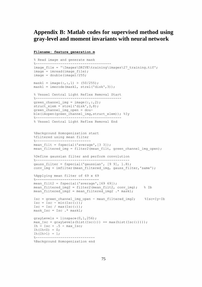
75

Appendix B: Matlab codes for supervised method using

gray-level and moment invariants with neural network

Filename: feature_generation.m

% Read image and generate mask

%-------------------------------------

image_file = '\Images\DRIVE\training\images\27_training.tif';

image = imread(image_file);

image = double(image)/255;

mask1 = image(:,:,1) > (50/255);

mask1 = imerode(mask1, strel('disk',3));

% Vessel Central Light Reflex Removal Start

%------------------------------------------

green_channel_img = image(:,:,2);

struct_elem = strel('disk',3,8);

green_channel_img_open = dou-

ble(imopen(green_channel_img,struct_elem)); %Iy

%------------------------------------------

% Vessel Central Light Reflex Removal End

%Background Homogenization start

%filtered using mean filter

%---------------------------

mean_filt = fspecial('average',[3 3]);

mean_filtered_img = filter2(mean_filt, green_channel_img_open);

%Define gaussian filter and perform convolution

%----------------------------------------------

gauss_filter = fspecial('gaussian', [9 9], 1.8);

conv_img = imfilter(mean_filtered_img, gauss_filter,'same');

%Applying mean filter of 69 x 69

%-------------------------------

mean_filt2 = fspecial('average',[69 69]);

mean_filtered_img2 = filter2(mean_filt2, conv_img); % Ib

mean_filtered_img2 = mean_filtered_img2 .* mask1;

Isc = green_channel_img_open - mean_filtered_img2; %Isc=Iy-Ib

Isc = Isc - min(Isc(:));

Isc = Isc / max(Isc(:));

mask_Isc = Isc .* mask1;

grayLevels = linspace(0,1,256);

max_Isc = grayLevels(hist(Isc(:)) == max(hist(Isc(:))));

Ih = Isc + .5 - max_Isc;

Ih(Ih<0) = 0;

Ih(Ih>1) = 1;

%-----------------------------

%Background Homogenization end

76

%Vessel Enhancement start

%------------------------

comp_Ih = imcomplement((Ih));

se = strel('disk', 8);

top_hat_trans_comp_Ih = imtophat(comp_Ih, se);

Ive = top_hat_trans_comp_Ih;

%----------------------

%Vessel Enhancement end

% Gray Level Based Feature Extraction

%------------------------------------

[f1, f2, f3, f4, f5] = gray_level_features(Ih);

% Moment Invariants Based Feature Extraction

%-------------------------------------------

f6 = nlfilter(Ive, [17 17], @moment_feature_vec_f6);

f7 = nlfilter(Ive, [17 17], @moment_feature_vec_f7);

%Naming the matfiles as 'Drive_image_27_features.mat'

%-------------------------------------------

mat_file = 'Drive_image_27_features.mat';

%Saving the features into separate matfiles

%-------------------------------------------

save(mat_file,'f1', 'f2', 'f3', 'f4', 'f5', 'f6', 'f7', '-v6');

Filename: gray_level_features.m

% Gray-Level-Based Features calculation

function [f1, f2, f3, f4, f5] = gray_level_features(Ih)

% fi => Features

% f1(x,y) = Ih(x,y) - min{Ih(s,t)}

fun1 = @(x) min(x(:));

Ih_min = nlfilter( Ih, [9 9], fun1);

f1 = Ih - Ih_min;

% f2(x,y) = max{Ih(s,t)} - Ih(x,y)

fun2 = @(x) max(x(:));

Ih_max = nlfilter( Ih, [9 9], fun2);

f2 = Ih_max - Ih;

% f3(x,y) = Ih(x,y) - mean{Ih(s,t)}

fun3 = @(x) mean(x(:));

Ih_mean = nlfilter( Ih, [9 9], fun3);

f3 = Ih - Ih_mean;

% f4(x,y) = Standard deviation{Ih(s,t)}

fun4 = @(x) std(x(:));

Ih_std = nlfilter( Ih, [9 9], fun4);

f4 = Ih_std;

% f5(x,y) = Ih(x,y)

f5 = Ih;

77

Filename: moment_feature_vec_f6.m

%First moment feature calculation

function f = moment_feature_vec_f6( I_ve)

%I_ve is vessel enhanced image

I_ve = double(I_ve);

gauss_matrix = fspecial('gaussian', [17 17], 1.7);

I_hu = I_ve .* gauss_matrix;

f = moment_features(I_hu, 6);

Filename: moment_feature_vec_f7.m

%Second moment feature calculation

function f = moment_feature_vec_f7( I_ve)

I_ve = double(I_ve);

gauss_matrix = fspecial('gaussian', [17 17], 1.7);

I_hu = I_ve .* gauss_matrix;

f = moment_features(I_hu, 7);

Filename: moment_features.m

%Moment features calculation

function f = moment_features(I_hu, count)

%I_hu is modified vessel enhanced image with a Gaussian filter

%count == 6 for sixth feature and count == 7 for seventh feature

if(count == 6)

% First Moment

n20 = normalized_central_moment(2, 0, I_hu);

n02 = normalized_central_moment(0, 2, I_hu);

phi_1 = n20 + n02;

f = abs(log(phi_1));

elseif(count == 7)

%Second Moment

n20 = normalized_central_moment(2, 0, I_hu);

n02 = normalized_central_moment(0, 2, I_hu);

n11 = normalized_central_moment(1, 1, I_hu);

phi_2 = (n20-n02)^2 + 4*(n11^2);

f = abs(log(phi_2));

else

error('Wrong input')

end

Filename: normalized_central_moment.m

function n_pq = normalized_central_moment( p, q, A)

%p = first order of moment

%q = second order of moment

%A = Modified vessel enhanced image (I_hu)

%if there is any 0's in image replace, it with very small number

%'eps'.

A(A == 0) = eps;

[m n] = size(A);

78

m00 = sum(sum(A));

%2-D Moment of order(p+q)

m10 = 0; % m_pq where p=1 and q=0

m01 = 0; % m_pq where p=0 and q=1

for a = 1:m

for b = 1:n

m10 = m10 + (a) * A(a,b);

m01 = m01 + (b) * A(a,b);

end

end

% Central moment

xx = m10/m00;

yy = m01/m00;

mu_00 = m00;

mu_pq = 0;

for ii = 1:m

x = ii-xx;

for jj = 1:n

y = jj-yy;

mu_pq = mu_pq + ((x)^p) * ((y)^q) * A(ii,jj);

end

end

% Normalized cental moment of order(p+q)

gamma = (0.5*(p+q))+1;

temp = (mu_00^(gamma));

n_pq = mu_pq/temp;

%if n_pq equals 0, assign it very less value 'eps'

n_pq(n_pq == 0) = eps;

Filename: train_data_generate.m

% Train and test data are generated in same way using this function

% Generate train data for NN load Drive_image_27_features.mat;

f1_mean = mean2(f1); f2_mean = mean2(f2); f3_mean = mean2(f3); f4_mean = mean2(f4); f5_mean = mean2(f5); f6_mean = mean2(f6); f7_mean = mean2(f7);

f1_std = std2(f1); f2_std = std2(f2); f3_std = std2(f3); f4_std = std2(f4); f5_std = std2(f5); f6_std = std2(f6); f7_std = std2(f7);

%Features normalized to zero mean and unit variance

79

new_f1 = (f1 - f1_mean)/f1_std; new_f2 = (f2 - f2_mean)/f2_std; new_f3 = (f3 - f3_mean)/f3_std; new_f4 = (f4 - f4_mean)/f4_std; new_f5 = (f5 - f5_mean)/f5_std; new_f6 = (f6 - f6_mean)/f6_std; new_f7 = (f7 - f7_mean)/f7_std;

train_data = [new_f1(:) new_f2(:) new_f3(:) new_f4(:) new_f5(:)

new_f6(:) new_f7(:)]; save('Drive_train_data_27.mat', 'train_data', '-v6');

Filename: target_data_generate.m

% Generates target data for training NN

manual = imread('\Images\DRIVE\training\1st_manual\27_manual1.gif'); manual_bw = (manual == 255); target_data = manual_bw(:); save('Drive_target_data_27.mat', 'target_data', '-v6');

Filename: trainedNN.m

% Training the NN

% Loads train and target data

load Drive_train_data_27.mat;

load Drive_target_data_27.mat;

%Training and target data are transposed to allow NN to take data as

%a column vector

train_data = train_data';

target_data = target_data';

netN = feedforwardnet(15);

net = train(netN, train_data, target_data);

mat_file = 'Drive_27_trainedNN.mat';

%Saving the trained NN into separate matfiles.

save(mat_file, 'net', '-v6');

Filename: simulationNN.m

%Perform simulation over the test data using trained NN

%load test data and trained NN

load Drive_test_data_02.mat;

load Drive_27_trainedNN.mat;

%read ground truth data

img = imread(‘\Images\DRIVE\test\1st_manual\02_manual1.gif’);

[row col] = size(img);

test_data = test_data';

% Simulation

Y = net(test_data);

80

% For DRIVE

threshold = (Y > 0.53);

% For STARE

%threshold = (Y > 0.43);

threshold = double(threshold);

reshape_threshold_img = reshape(threshold, row, col);

final_segmented_image = post_processing(reshape_threshold_img);

figure, imshow(final_segmented_image);

final_segmented_image = double(final_segmented_image);

[Se, Sp, ppv, Npv, Acc] = performance_measure(final_segmented_image,

img)

Filename: post_processing.m

% Post Processing step

function x = post_processing(I)

%I = segmented image

%Iterative filling; at least neighbor 6 pixels must be vessel to

%consider a center pixel as a vessel

fill = nlfilter(I, [6 6], @iterative_fill);

%artifact removal: Each connected region to an area below 10 is

%reclassified as non-vessels

final_vessel_segmented_image = bwareaopen(fill, 10);

x = final_vessel_segmented_image;

Filename: performance_measure.m

function [Se, Sp, Ppv, Npv, Acc] = performance_measure(final_image,

target_image)

% Se = Sensitivity

% Sp = Specificity

% Ppv = Positive predictive value

% Npv = Negative predictive value

% Acc = Accuracy

% final_image = post processed final image

% target_image = gold standard image

TP = 0; %True Positive

FP = 0; %False Positive

FN = 0; %False Negative

TN = 0; %True Negative

[row col] = size(target_image);

target_image = im2bw(target_image);

for x = 1:row

for y = 1:col

if((final_image(x,y)== 1) && (target_image(x,y) == 1))

TP = TP + 1;

else if((final_image(x,y)== 1) && (target_image(x,y) == 0))

FP = FP + 1;

else if((final_image(x,y)==0)&&(target_image(x,y) ==1))

81

FN = FN + 1;

else

TN = TN + 1;

end

end

end

end

end

Se = TP /(TP + FN);

Sp = TN /(TN + FP);

Ppv = TP /(TP + FP);

Npv = TN /(TN + FN);

Acc = (TP + TN)/(TP + FN + TN + FP);

82

Appendix C: Matlab codes for unsupervised method us-

ing local entropy and gray-level co-occurrence matrix

Filename: Main_unsupervised_method.m

% Main method

img = imread('\Images\DRIVE\test\images\01_test.tif');

img = img(:,:,2);

img = double(img)/255;

mask = img > (20/255); % For Drive

%mask = img > (35/255); % For stare

mask = double(imerode(mask, strel('disk',3)));

% Matched filtering

extractedVessel = MatchFiltered(img, 1.2, 9, 12);

% Element-wise multiplication

newExtractedVessel = extractedVessel.*mask;

% Normalization

normVessel = newExtractedVessel - min(newExtractedVessel(:));

normVessel = normVessel / max(normVessel(:));

normVessel = round(normVessel * 255);

grayValue = (unique(normVessel(:)))';

grayValueCount = numel(grayValue);

c = grayValueCount;

t = graycomatrix(newExtractedVessel, 'GrayLimits',

[min(newExtractedVessel(:)) max(newExtractedVessel(:))], 'Num-

Levels', c);

% Adding entire values of the co-occurence matrix

t_sum = sum(t(:));

% Normalizing the co-occurrence matrix

P = zeros(c,c);

for i = 1:c

for j = 1:c

P(i,j) = t(i,j)/t_sum;

end

end

t_JRE = generate_Tjre(P, c);

% Thresholding

final_segmented_img = newExtractedVessel > t_JRE;

g_truth = imread('\Images\DRIVE\test\1st_manual\01_manual1.gif');

% performance_measure function is same as used in supervised method

[Se, Sp, Ppv, Npv, Acc] = performance_measure(final_segmented_img,

g_truth);

83

Filename: matched_filtered.m

function[vess] = match_filtered(img,sigma,yLengthForMF, numOfDirec-

tions) % Retinal vessel extraction by matched filter % % Inputs: % img - input imgage % sigma - scale value % yLengthForMF - length of neighborhood along y-

% axis of MF % numOfDirections - number of orientations % % Output: % vess - vessels extracted

if isa(img, 'double')~=1 img = double(img); end

[rows, cols] = size(img);

MatchFilterRes(rows, cols, numOfDirections) = 0; for i = 0:numOfDirections-1

matchFilterKernel = match_filter_kernel_generate(sigma, yLength-

ForMF, pi/numOfDirections*i); MatchFilterRes(:,:,i+1) = conv2(img, matchFilterKernel, 'same'); end

[maxMatchFilterRes] = max(MatchFilterRes, [], 3); vess = maxMatchFilterRes;

Filename: match_filter_kernel_generate.m

function[kernel]=match_filter_kernel_generate(sigma, YLength, theta) % MF kernel construction % % Inputs: % sigma - scale value % YLength - length of neighborhood along y-axis % theta - orientation % % Output: % kernel - MF kernel % % YLength should be an odd integer

widthOfTheKernel = ceil(sqrt( (6*ceil(sigma)+1)^2 + YLength^2)); if mod(widthOfTheKernel,2) == 0 widthOfTheKernel = widthOfTheKernel + 1; end halfLength = (widthOfTheKernel - 1) / 2; row = 1; for y = halfLength:-1:-halfLength col = 1;

84

for x = -halfLength:halfLength xPrime = x * cos(theta) + y * sin(theta); yPrime = y * cos(theta) - x * sin(theta); if abs(xPrime) > 3.5*ceil(sigma) matchFilterKernel(row,col) = 0; elseif abs(yPrime) > (YLength-1) / 2 matchFilterKernel(row,col) = 0; else

matchFilterKernel(row,col) = -exp(-.5*(xPrime/sigma)^2)

/ (sqrt(2*pi)*sigma); end col = col + 1; end row = row + 1; end mean = sum(sum(matchFilterKernel))/sum(sum(matchFilterKernel < 0)); for i = 1:widthOfTheKernel for j =1:widthOfTheKernel if matchFilterKernel(i,j) < 0 matchFilterKernel(i,j) = matchFilterKernel(i,j) - mean; end end end kernel = matchFilterKernel;

Filename: generate_Tjre.m

function T = new_generate_Tjre( P, L)

%% Probabilities associated with each quadrants

x = 1;

T_JRE = zeros(L);

for th = 1:L

PtB = sum(sum(P(1:th, th+1:L)));

PtD = sum(sum(P(th+1:L, 1:th)));

qtB = PtB / ((th+1)*(L-th-1));

qtD = PtD / ((L-th-1)*(L+1));

temp = -( PtB*log(qtB) + PtD*log(qtD))/10;

if temp > 0

T_JRE(x) = temp;

x = x + 1;

end

end

T = max(T_JRE(:));

end

85

Appendix D: Matlab codes for matched filtering method

using first order derivative of Gaussian

Filename: Main_matched_filtering_method.m

img = imread('\Stare\StareImages\im0162.ppm\im0162.ppm');

img = img(:,:,2);

% Mask for the fundus image generation

level = graythresh(img) - 0.06;

mask = im2bw(img,level);

gTruth = imread('\Stare\labels-ah\im0162.ah.ppm\im0162.ah.ppm');

se = strel('disk',4);

mask=imerode(mask,se);

%MatchFilterWithGaussDerivative(image, sigma, yLength, numOfDirec-

tions, mask, c_value, threshold value_for_regionprop)

thick_vess = MatchFilterWithGaussDerivative(img, 1.5, 9, 12, mask,

2.3, 30);

figure, imshow(thick_vess)

thin_vess = MatchFilterWithGaussDerivative(img, 1, 4, 12, mask, 2.3,

30);

figure, imshow(thin_vess)

vess = thick_vess | thin_vess;

figure, imshow(vess)

[tpr tnr acc] = performance_measure(vess, mask, gTruth)

Filename: MatchFilterWithGaussDerivative.m

function [vess] = MatchFilterWithGaussDerivative(img, sigma,

yLength, numOfDirections, mask, c_value, t)

% Retinal vessel extraction by matched filter with first-order

% derivative of Gaussian

%

% Inputs:

% img - input imgage

% sigma - scale value

% yLength - length of neighborhood along y-

% axis

% numOfDirections - number of orientations

% mask - image mask

% c_value - c value

% t - threshold value of region props

%

% Output:

% vess - vessels extracted

if isa(img,'double')~=1

img = double(img);

end

86

[rows,cols] = size(img);

MatchFilterRes(rows,cols,numOfDirections) = 0;

GaussDerivativeRes(rows,cols,numOfDirections) = 0;

for i = 0:numOfDirections-1

matchFilterKernel = MatchFilterAndGaussDerKernel(sigma,

yLength, pi/numOfDirections*i, 0);

gaussDerivativeFilterKernel = MatchFilterAndGaussDerKer-

nel(sigma, yLength, pi/numOfDirections*i, 1);

MatchFilterRes(:,:,i+1) = conv2(img,matchFilterKernel,'same');

GaussDerivativeRes(:,:,i+1) =

(conv2(img,gaussDerivativeFilterKernel,'same'));

end

maxMatchFilterRes = max(MatchFilterRes,[],3);

maxGaussDerivativeRes = max(GaussDerivativeRes,[],3);

D = maxGaussDerivativeRes;

W = fspecial('average', 31);

Dm = imfilter(D, W);

%Normailzation

Dm = Dm - min(Dm(:));

Dm = Dm/max(Dm(:));

%muH = mean value of response image H

H = maxMatchFilterRes;

c = c_value;

muH = mean(H(:));

Tc = c * muH;

T = (1 + Dm) * Tc;

Mh = (H >= T);

vess = Mh & mask;

se = strel('square',3);

vess = imclose(vess,se);

vess = bwmorph(vess,'close');

[L num] = bwlabel(vess, 8);

prop = regionprops(L, 'Area');

idx = find([prop.Area] > t);

vess = ismember(L,idx);

Filename: MatchFilterAndGaussDerKernel.m

function [kernel] = MatchFilterAndGaussDerKernel(sigma, YLength,

theta, type)

%

% MF and FDOG kernel construction

%

% Inputs:

% sigma - scale value

% YLength - length of neighborhood along y-axis

87

% theta - orientation

% type - MF or FDOG

%

% Output:

% kernel - Gaussian kernel

if type == 0

widthOfTheKernel = ceil(sqrt((6*ceil(sigma)+1)^2 + YLength^2));

if mod(widthOfTheKernel,2) == 0

widthOfTheKernel = widthOfTheKernel + 1;

end

halfLength = (widthOfTheKernel - 1) / 2;

row = 1;

for y = halfLength:-1:-halfLength

col = 1;

for x = -halfLength:halfLength

xPrime = x * cos(theta) + y * sin(theta);

yPrime = y * cos(theta) - x * sin(theta);

if abs(xPrime) > 3.5*ceil(sigma)

matchFilterKernel(row,col) = 0;

elseif abs(yPrime) > (YLength-1) / 2

matchFilterKernel(row,col) = 0;

else

matchFilterKernel(row,col) = -exp(-

.5*(xPrime/sigma)^2)/(sqrt(2*pi)*sigma);

end

col = col + 1;

end

row = row + 1;

end

mean=sum(sum(matchFilterKernel))/sum(sum(matchFilterKernel<0));

for i = 1:widthOfTheKernel

for j =1:widthOfTheKernel

if matchFilterKernel(i,j) < 0

matchFilterKernel(i,j)=matchFilterKernel(i,j)- mean;

end

end

end

kernel = matchFilterKernel;

else

widthOfTheKernel = ceil(sqrt( (6*ceil(sigma)+1)^2 + YLength^2));

if mod(widthOfTheKernel,2) == 0

widthOfTheKernel = widthOfTheKernel + 1;

end

halfLength = (widthOfTheKernel - 1) / 2;

row = 1;

for y = halfLength:-1:-halfLength

col = 1;

for x = -halfLength:halfLength

xPrime = x * cos(theta) + y * sin(theta);

yPrime = y * cos(theta) - x * sin(theta);

if abs(xPrime) > 3.5*ceil(sigma)

GaussDerivativeKernel(row,col) = 0;

elseif abs(yPrime) > (YLength-1) / 2

GaussDerivativeKernel(row,col) = 0;

else

88

GaussDerivativeKernel(row,col)= -exp(-

.5*(xPrime/sigma)^2)*xPrime/(sqrt(2*pi)*sigma^3);

end

col = col + 1;

end

row = row + 1;

end

kernel = GaussDerivativeKernel;

end

Filename: performance.m

function [tpr fpr accu] = performance(img, mask, gTruth) % % Performance measurement % % Inputs: % img - input image % mask - image mask % gTruth - ground truth % % Outputs: % tpr - true positive rate % fpr - false positive rate % accu - accuracy

img = logical(img); mask = logical(mask); gTruth = logical(gTruth); [index] = find(mask(:) == 1); tpr = sum(gTruth(img(:) == 1)) / sum(gTruth(index) == 1); accu = sum(img(index) == gTruth(index)) / length(index); fpr = sum(gTruth(img(:) == 1 & mask(:) == 1) == 0) /

sum(gTruth(index) == 0);