Blioumi, Smilauer: Cross-anisotropic Rock Modelled with Discrete Methods (EURO:TUN 2013)

EURO:TUN 2013

3rd International Conference on Computational Methods in Tunneling and Subsurface Engineering Ruhr University Bochum, 17-19 April 2013

397

Cross-anisotropic Rock Modelled with Discrete Methods

Václav Šmilauer1 and Anastasia Blioumi1 1University of Innsbruck, Department of Geotechnical and Tunnel Engineering,

Innsbruck, Austria

Abstract

In rock-engineering practice, layered rocks with cross-anisotropic features are

frequently encountered. Alpine tunnel construction sites are often confronted with

problems related to cross-anisotropic rocks like phyllites and schists. The assumption

of isotropic behaviour is not acceptable to realistically describe the behaviour of such

rocks. Rising popularity of discrete methods calls for an appropriate formulation of

such materials within their framework. Analytical derivation of parameters of lattice

structure which globally exhibits cross-anisotropic behaviour is presented. For this

purpose, directionally isotropic lattice, of which links transmit normal and shear load,

is considered. Normal and shear stiffnesses are derived as functions of link orientation

in such a way that globally observed elastic behaviour recovers cross-anisotropic

properties of the continuum. The procedure is based on employing the microplane

model as a limit of isotropic and infinitely dense lattice. The result is still a good

approximation of less ideal lattices. The aforementioned lattice arrangements can be

found as contact configuration in spherical packings used in the Discrete Element

Method. Discrete elements with orientation-dependent stiffness are used to show

match between theoretically predicted global moduli and behaviour during element

tests. A circular tunnel in cross-anisotropic rock subject to radial pressure is also

simulated with discrete elements.

Keywords: Rock mechanics, cross-anisotropy, discrete methods

Václav Šmilauer and Anastasia Blioumi

398

1 INTRODUCTION

Rocks composed of parallel layers (sedimentation or schistosity, e.g. slates and

schists) belong to the cross-anisotropic materials (often referred as transversely

isotropic or as transverse isotropic materials). In Austria, this subject is of great

interest. A great number of tunnel projects, among them the European infrastructure

project of Brenner base tunnel, are currently under constructions. These Tunnels must

be totally or partly driven through cross-anisotropic rocks like schiefer, quarz phyllite,

black phyllite and Bündner schist which are typical for the Alp region.

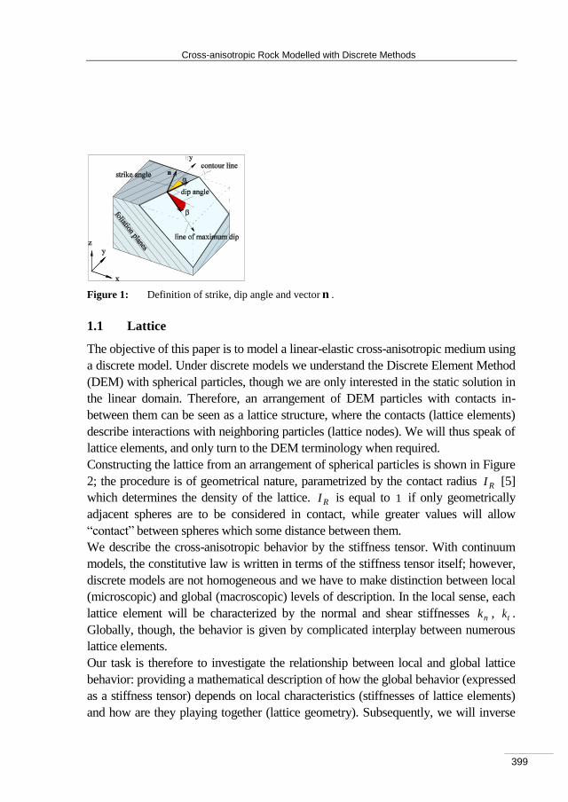
To define the orientation of the foliation planes in the 3-D space, the strike angle

and the dip angle are used. The different definitions of these angles found in the

literature can be puzzling. The authors used following definitions (see Figure 1)strike

angle is the clock-wise angle between the axis y and the contour line, i.e. the line

obtained from the intersection of the foliation plane with a horizontal one. The y -axis

coincides with the axis of the considered cylindrical cavity, e.g. tunnel or drill-hole.

Dip angle is the smallest angle between a horizontal line which is perpendicular to

the contour line and the line of maximum dip of the foliation plane.

Cross-anisotropic materials exhibit rotational symmetry in mechanical response about

the unit vector n normal to the foliation (Figure 1). This means that the material is

isotropic in the plane normal to this vector. For the case where n coincides with the

global z -axis, this symmetry is captured by the stiffness tensor

(1)

with five independent components.

In the Cartesian coordinate system x , y , z , n is given, in respect to the angles and

, as )cos,sinsin,sincos(= n .

200000

00000

00000

000

000

000

=

1211

44

44

331313

131112

131211

CC

C

C

CCC

CCC

CCC

C


399

Figure 1: Definition of strike, dip angle and vector n .

1.1 Lattice

The objective of this paper is to model a linear-elastic cross-anisotropic medium using

a discrete model. Under discrete models we understand the Discrete Element Method

(DEM) with spherical particles, though we are only interested in the static solution in

the linear domain. Therefore, an arrangement of DEM particles with contacts in-

between them can be seen as a lattice structure, where the contacts (lattice elements)

describe interactions with neighboring particles (lattice nodes). We will thus speak of

lattice elements, and only turn to the DEM terminology when required.

Constructing the lattice from an arrangement of spherical particles is shown in Figure

2; the procedure is of geometrical nature, parametrized by the contact radius RI [5]

which determines the density of the lattice. RI is equal to 1 if only geometrically

adjacent spheres are to be considered in contact, while greater values will allow

“contact” between spheres which some distance between them.

We describe the cross-anisotropic behavior by the stiffness tensor. With continuum

models, the constitutive law is written in terms of the stiffness tensor itself; however,

discrete models are not homogeneous and we have to make distinction between local

(microscopic) and global (macroscopic) levels of description. In the local sense, each

lattice element will be characterized by the normal and shear stiffnesses nk , tk .

Globally, though, the behavior is given by complicated interplay between numerous

lattice elements.

Our task is therefore to investigate the relationship between local and global lattice

behavior: providing a mathematical description of how the global behavior (expressed

as a stiffness tensor) depends on local characteristics (stiffnesses of lattice elements)

and how are they playing together (lattice geometry). Subsequently, we will inverse


400

the previous result, i.e. for some desired stiffness tensor, we will determine local

characteristics (stiffnesses) leading to the behavior described by that tensor.

To this end, we make use of the following assumptions: the lattice is isotropic, i.e. the

orientation of the lattice elements is in average uniformly distibuted; the displacement

of lattice nodes does not deviate from the mean displacement, in another words, the

lattice is deformed uniformly, as whole. The latter is commonly referred to as Voigt

hypothesis [4] and is an important restriction for the lattice behavior. Denser lattices

(with greater RI ) fulfill this assumption by themselves better than loose lattices, as

they have more contacts restricting deviation of individual nodes from the

surrounding deformation. We therefore expect our results to better describe the real

behavior in the case of dense lattices.

Figure 2: Dependence of lattice density on contact radius RI : (a) sphere packing for

constructing the lattice, (b) lattice with small RI , (c) lattice with bigger RI

1.2 Microplane and Lattice

The transition between discrete, i.e. lattice [3] and continuous description will be done

via the microplane theory [2]. This theory describes each material point as an infinite

number of microplanes oriented uniformly in all possible directions at that material

point, each of them characterized by volumetric, deviatoric, normal and shear moduli

(in our case, we only use the latter two, NE and TE ). The cross-anisotropic nature is

introduced by supposing dependency of those moduli on the respective microplane

orientation such that symmetries of a cross-anisotropic medium are satisfied. The

stiffness tensor is obtained by integration of the moduli over all microplanes.

The lattice structure has only a finite number of nodes and a finite number of

isotropically-oriented lattice elements in each node. The stiffness tensor is obtained by

summation of stiffnesses over all elements. We can write the lattice stiffnesses nk , tk

as functions of some yet unknown moduli NE , TE and let the lattice density grow


401

without bounds. After limit transition, we obtain the stiffness tensor of the infinitely

dense lattice by integration of the unknown moduli over all lattice elements.

By imposing equality of microplane and lattice sttiffness tensors, we obtain the values

of the unknown lattice moduli NE , TE (proportional to the microplane moduli);

using those moduli when constructing the lattice ensures that the stiffness tensor of

the discrete lattice will be equal to the stiffness tensor of the microplane model.

Consequently, for a given stiffness tensor, we can compute lattice moduli which will

lead to the response characterized by that stiffness tensor.

1.3 Tests

The stiffness tensor of a lattice is obtained from element tests (in our case, uniaxial

unconfined compression and simple shear tests) on a periodic lattice. It is

subsequently compared with the prescribed values, and the dependence between

accuracy and lattice density is shown. The second numerical example is modeling of

a tunnel subjected to radial pressure. For space reasons, this paper does not show all

steps of the derivation in form of equations. These will be soon published separately.

2 NOTATION

NE , TE : microplane normal and tangential moduli

NE , TE : lattice normal and tangential moduli

nk , tk : lattice normal and tangential stiffnesses

mnC : stiffness matrix component

)0,2 : azimuth angle in spherical coordinates

)0, : inclination angle in spherical coordinates, from the pole

3 MICROPLANE STIFFNESS

We consider the microplane model by [2] where all microplanes only have normal

and shear moduli NE , TE . The stiffness tensor is obtained by integration of the

moduli over all possible orientations of microplanes given by the unit vector n . For

our purposes, we will integrate over angles , (Figure 3.a), z -axis being

coincident with the cross-anisotropy axis; this lets us write microplane moduli as

)(= NN EE and )(= TT EE , independent of the azimuth . We will assume that

those moduli can be given as combination of in-plane ( aNE , a

TE ) and out-of-plane (bNE , b

TE ) ones,


402

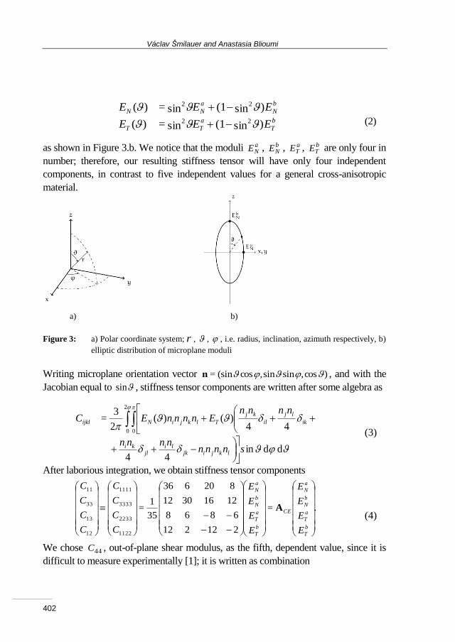
(2)

as shown in Figure 3.b. We notice that the moduli aNE , b

NE , aTE , b

TE are only four in

number; therefore, our resulting stiffness tensor will have only four independent

components, in contrast to five independent values for a general cross-anisotropic

material.

a) b)

Figure 3: a) Polar coordinate system; r , , , i.e. radius, inclination, azimuth respectively, b)

elliptic distribution of microplane moduli

Writing microplane orientation vector )cos,sinsin,cossin(= n , and with the

Jacobian equal to sin , stiffness tensor components are written after some algebra as

(3)

After laborious integration, we obtain stiffness tensor components

(4)

We chose 44C , out-of-plane shear modulus, as the fifth, dependent value, since it is

difficult to measure experimentally [1]; it is written as combination

b

T

a

TT

b

N

a

NN

EEE

EEE

)sin(1sin=)(

)sin(1sin=)(22

22

d d in44

44)()(

2

3=

0

2

0

snnnnnnnn

nnnnEnnnnEC

lkjijkli

jlki

ik

lj

il

kj

TlkjiNijkl

.=

212212

6868

12163012

820636

35

1=

1122

2233

3333

1111

12

13

33

11

b

T

a

T

b

N

a

N

CE

b

T

a

T

b

N

a

N

E

E

E

E

E

E

E

E

C

C

C

C

C

C

C

C

A


403

(5)

The matrix CEA in Eq. (4) is invertible; thus we obtain the solution of the inverse

problem (when ijC are given) as

4 MICROPLANE-LATTICE MODULI PROPORTION

Components of the stiffness tensor were derived for microplane moduli NE , TE ,

which are necessarily proportional to lattice contact moduli NE , TE via a

dimensionless factor , which expresses relative “stiffness density” of the lattice, and

has a geometrical meaning shown below. We will show the derivation only for the

normal moduli; the procedure for tangential moduli is identical.

Considering lattice constructed from spherical packing, we suppose intra-nodal

stiffnesses given as )/(2= 2 rrEk Nn , where 2r is a fictious contact area, divided by

contact length r2 . In general rrEk Nn /ˆ= 2 with some algorithm-dependent constant

(we assume no special value of , in the case mentioned it is equal to /2 ).

Microplane moduli are then related to intra-nodal stiffess via some unknown as

(7)

To find the value of value, we suppose that the lattice is in average isotropic, i.e.

lattice element length r2 is in average orientation-independent; the difference

between r and r accounts for possibly non-unit contact radius RI as explained

above (Figure 2). The lattice occupies volume V and has N contacts, the only

orientation-dependent values are the moduli )(' NE and )(' TE .

By comparing stiffness tensors for lattice after limit transition (Eq. (38) in [3]) with

microplane stiffness integral, we obtain, with some algebra,

(8)

with 2rr denoting the average value of 2rr over all contacts.

.

8

13

6

8

35

1=

0

1/2

1/4

1/4

=

12

13

33

11

232344

b

T

a

T

b

N

a

N

TT

E

E

E

E

C

C

C

C

CC

.=

12

13

33

11

1

C

C

C

C

E

E

E

E

CE

b

T

a

T

b

N

a

N

A

.=/ˆ== 2

NNnN ErrEkE

V

rrN

E

E

E

E

T

T

N

N

ˆ

3

2=

'=

'=

2


404

The geometrical meaning of the equation can be seen better if we consider the special

case of both r and r being constant; averages can be then omitted, giving

(9)

We see that is dimensionless, giving proportion of N contact “volumes” (area 2ˆ2= rAi , length rli 2= ) to the overall lattice volume V .

Since all relationships for )( *ECij in (4) are linear in *E , macroscopic lattice stiffness

can be written as )(=)( ** ECEC ijij . In particular, the Eq. (4) and its inverse become

(10)

5 ELEMENT TESTS

Random dense (porosity equal to 0.5) periodic packing of spheres with equal radius is

considered. The lattice structure is created by finding contacts between particles,

using varying contact radius RI . The cross-anisotropy axis coincides with the global

z -axis. Given laboratory values of 11C , 33C , 13C , 12C , we use the current packing

geometry to determine and lattice moduli via Eq. (10) and assign stiffnesses via

Eq. (2). The goal is to compare the stiffness tensor obtained in three different ways:

the prescribed values (back-calculated from lattice stiffnesses); from the current

lattice by summation of stiffnesses, using Eq. (35) in [3]; from simulated lattice

response, with stiffnesses in Eq. (10), loaded in different ways, as decribed below.

The test is run for a range of contact radii RI , to show that denser lattice has a

stabilizing effect, being closer to the Voigt hypothesis, as mentioned in the

introduction.

5.1 Computing the Stiffness Tensor

We simulate homogeneous loading of periodic lattice structure to obtain parameters of

the cross-anisotropic material. For each axis, we perform an unconfined uniaxial

compression test to obtain normal modulus and Poisson’s ratios, and a shear test to

obtain shear modulus (Figure 4). In total, six tests are run. Out of the 12 values obtained

(three normal moduli, three shear moduli, three Poisson’s ratios, each measured twice),

only five are independent; redundant values are used to check correctness.

.)(

6

1=

)ˆ)(2(2

6

1=

2

V

AlN

V

rrN ii

.1

=

'

'

'

'

,

'

'

'

'

=

12

13

33

11

1

12

13

33

11

C

C

C

C

E

E

E

E

E

E

E

E

C

C

C

C

CE

b

T

a

T

b

N

a

N

b

T

a

T

b

N

a

N

CE AA


405

Figure 4: Configuration of (a) unconfined uniaxial compression test in the y -direction and (b)

shear test in the xy plane

5.1.1 Normal moduli and Poisson’s ratios

To find normal moduli from simulations, we make use of the normal compliance

relationship for orthotropic material, of which cross-anisotropic material is a special

case:

(11)

and prescribe strain in one direction with zero lateral stresses and evaluate the

response. For instance, for the x -compression we prescribe (prescribed values are

denoted with ˆ)

(12)

and use measured response xx , yy , zz to compute

(13)

5.1.2 Shear moduli

The shear test is purely deformation-controlled. The periodic cell is prescribed shear

strain . Shear moduli are found from shear stiffness equations.

zz

yy

xx

zy

yz

x

xz

z

zy

yx

xy

z

zx

y

yx

x

zz

yy

xx

EEE

EEE

EEE

1

1

1

=

0,==,ˆ=ˆ= zzyyxxxx

.ˆ

=,ˆ

==,ˆ

=xx

zzxz

xx

yy

xx

xyyxy

xx

xxx

EE


406

(14)

5.1.3 Stiffness tensor

Components of the stiffness tensor are found by inversion of the orthotropic

compliance matrix in Eq. (11) using symmetries xy EE = , yzxz = and abbreviating

zx EEe /= , 221= xzxy em :

5.2 Results

Values of input parameters for 1.8=RI are shown in Table 1. Resulting stiffnesses

for all values of RI are given in Table 2. As expected, higher values of RI lead to a

better agreement with simulated results.

Table 1: Input and derived values for the six element tests performed for 1.8=RI .

Input values Derived values

number of spheres 1060 avg. number of contacts per sphere 21

sphere radius (m) 0.04 lattice density scaling 1.89

interaction radius rI 1.8 'aNE (MPa) 64.1

11C (MPa) 130 'bNE (MPa) 6.37

33C (MPa) 55 'aTE (MPa) 3.05

13C (MPa) 28 'bTE (MPa) 1.06

12C (MPa) 40

prescribed strain 1%

.=ˆ2

=,,=2ij

ij

ij

ij

ij

ij

ij

ij GjiG

.

1

)(1

)(1

1

=

2

2

44

33

13

12

11

yz

xy

z

xy

x

xy

xzxy

x

xy

xzx

Gm

E

mE

m

eE

m

eE

C

C

C

C

C


407

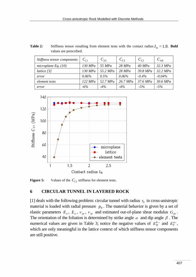
Table 2: Stiffness tensor resulting from element tests with the contact radius 1.8=RI . Bold

values are prescribed.

Stiffness tensor components 11C 33C

13C 12C

44C

microplane Eq. (10) 130 MPa 55 MPa 28 MPa 40 MPa 32.3 MPa

lattice [3] 130 MPa 55.2 MPa 28 MPa 39.8 MPa 32.2 MPa

error 0.06% 0.5% 0.06% -0.4% -0.04%

element tests 122 MPa 52.7 MPa 26.7 MPa 37.6 MPa 30.6 MPa

error -6% -4% -4% -5% -5%

Figure 5: Values of the 11C stiffness for element tests.

6 CIRCULAR TUNNEL IN LAYERED ROCK

[1] deals with the following problem: circular tunnel with radius 0r in cross-anistropic

material is loaded with radial pressure 0p . The material behavior is given by a set of

elastic parameters xE , zE , xy , xz and estimated out-of-plane shear modulus yzG .

The orientation of the foliation is determined by strike angle and dip angle . The

numerical values are given in Table 3; notice the negative values of 'bNE and 'a

TE ,

which are only meaningful in the lattice context of which stiffness tensor components

are still positive.


408

Table 3: Input and derived values for the circular tunnel problem.

Input values Derived values

number of spheres 9100 average number of contacts 14.5

sphere radius (m) 0.24 lattice density scaling 1.32

interaction radius rI 1.5 'a

NE (GPa) 4

foliation strike angle 270° 'b

NE (MPa) -70

foliation dip angle 25° 'a

TE (MPa) -26.5

xE (GPa) 5 'b

TE (GPa) 1.17

zE (GPa) 2 2G =yzG (lattice) (GPa) 1.52

xy

0.25

xz

0.125

yzG (estimate) (GPa) 1.21

0p (MPa) 5

Stiffness tensor components are computed using Eq. (15). Lattice moduli (Eq. (10))

are used with Eq. (2) to obtain stiffnesses for the individual lattice elements. Scaling

parameter in Eq. (7) is computed from the geometrical arrangement via Eq. (9).

The DEM model consists of a regular arrangement of particles at the tunnel wall,

while the rest of the medium is the result of random central-attraction deposition.

Particle radius was chosen such that the tunnel wall has 20 particles around the

perimeter. Simulated domain was cropped circularly to 010 r , and is periodic along

the tunnel axis. All particles (including the ones on the boundaries) are free to move.

The pressure 0p is applied on the tunnel wall as force on each of the particles. The

resulting deformation curve, shown in Figure 5, corresponds qualitatively to the

results of [1] obtained with the finite element method.


409

Figure 6: Radial displacements of the tunnel wall (innermost layer of particles).

7 CONCLUSIONS

A method of capturing cross-anisotropic behavior with discrete lattice-like models

was presented. We have established relationship between the moduli of dense lattices

and the microplane model under the assumption of the Voigt hypothesis and elliptical

distribution of orientation-dependent stiffnesses. This relationship let us determine

local lattice stiffnesses so that the global behavior corresponds to the desired stiffness

tensor; the agreement depends on the density of the lattice, which is given by the

contact radius RI ; larger values of RI give very good agreement. An example of

deformation of circular tunnel in layered rock subject to radial pressure was given.

Thus, our results find an application in modelling deformation of layered rock with

discrete models, which are becoming increasingly popular in engineering practice.


410

ACKNOWLEDGEMENTS

The authors wish to thank the Austrian Science of Fund (FWF): I 703-N22 for the

financial support.

REFERENCES

[1] Blioumi A. On Linear-Elastic, Cross-Anisotropic Rock. PhD thesis, Faculty

of Civil Engineering of the University of Innsbruck, 2011.

[2] Carol I., Jirásek M. & Bazant Z. P. A framework for microplane models at

large strain, with application to hyperelasticity. International Journal of

Solids and Structures Vol. 410 (2), (2004), 511-557.

[3] Kuhl E., D'Addetta G. A., Leukart M. & Ramm E. Microplane modelling

and particle modelling of cohesive-frictional materials. In Continuous and

Discontinuous Modelling of Cohesive-Frictional Materials, Vol. 568 of

Lecture Notes in Physics, (2001), 31-46. Berlin / Heidelberg: Springer

[4] Liao C.-L., Chang T.-P., Young D.-H. & Chang C. S. Stress-strain

relationship for granular materials based on the hypothesis of best fit.

International Journal of Solids and Structures, Vol. 340 (31-32), (1997),

4087-4100.

[5] Stránský J., Jirásek M. & Šmilauer V. Macroscopic elastic properties of

particle models. In Proc. of the International Conference on Modelling and

Simulation 2010, Prague, June 2010.

Blioumi, Smilauer: Cross-anisotropic Rock Modelled with Discrete Methods (EURO:TUN 2013)

Documents

Transcript of Blioumi, Smilauer: Cross-anisotropic Rock Modelled with Discrete Methods (EURO:TUN 2013)