BlinkDB: Queries with Bounded Errors andBounded Response Times on Very Large Data

Sameer Agarwal†, Barzan Mozafari○, Aurojit Panda†, Henry Milner†, Samuel Madden○, Ion Stoica∗†

†University of California, Berkeley ○Massachusetts Institute of Technology ∗Conviva Inc.{sameerag, apanda, henrym, istoica}@cs.berkeley.edu, {barzan, madden}@csail.mit.edu

AbstractIn this paper, we present BlinkDB, a massively parallel, ap-proximate query engine for running interactive SQL querieson large volumes of data. BlinkDB allows users to trade-o� query accuracy for response time, enabling interactivequeries overmassive data by running queries on data samplesand presenting results annotated with meaningful error bars.To achieve this, BlinkDB uses two key ideas: (1) an adaptiveoptimization framework that builds and maintains a set ofmulti-dimensional strati�ed samples from original data overtime, and (2) a dynamic sample selection strategy that selectsan appropriately sized sample based on a query’s accuracy orresponse time requirements.We evaluateBlinkDB against thewell-known TPC-H benchmarks and a real-world analyticworkload derived from Conviva Inc., a company that man-ages video distribution over the Internet. Our experimentson a 100 node cluster show that BlinkDB can answer querieson up to 17 TBs of data in less than 2 seconds (over 200× fasterthan Hive), within an error of 2-10%.

1. IntroductionModern data analytics applications involve computing aggre-gates over a large number of records to roll-up web clicks,online transactions, content downloads, and other featuresalong a variety of di�erent dimensions, including demo-graphics, content type, region, and so on. Traditionally, suchqueries have been executed using sequential scans over alarge fraction of a database. Increasingly, new applicationsdemand near real-time response rates. Examplesmay includeapplications that (i) update ads on a website based on trendsin social networks like Facebook and Twitter, or (ii) deter-mine the subset of users experiencing poor performancebased on their service provider and/or geographic location.Over the past two decades a large number of approxima-

tion techniques have been proposed, which allow for fast pro-

Permission to make digital or hard copies of all or part of this work for personalor classroom use is granted without fee provided that copies are not made ordistributed for profit or commercial advantage and that copies bear this noticeand the full citation on the first page. To copy otherwise, to republish, to poston servers or to redistribute to lists, requires prior specific permission and/or afee.Eurosys’13 April 15-17, 2013, Prague, Czech RepublicCopyright © 2013 ACM 978-1-4503-1994-2/13/04. . . $15.00

cessing of large amounts of data by trading result accuracyfor response time and space.�ese techniques include sam-pling [10, 14], sketches [12], and on-line aggregation [15]. Toillustrate the utility of such techniques, consider the followingsimple query that computes the average SessionTime overall users originating in New York:

SELECT AVG(SessionTime)

FROM Sessions

WHERE City = ‘New York’

Suppose the Sessions table contains 100 million tuples forNew York, and cannot �t in memory. In that case, the abovequerymay take a long time to execute, since disk reads are ex-pensive, and such a query would need multiple disk accessesto stream through all the tuples. Suppose we instead exe-cuted the same query on a sample containing only 10, 000New York tuples, such that the entire sample �ts in mem-ory.�is would be orders of magnitude faster, while still pro-viding an approximate result within a few percent of the ac-tual value, an accuracy good enough for many practical pur-poses. Using sampling theory we could even provide con�-dence bounds on the accuracy of the answer [16].Previously described approximation techniques make dif-

ferent trade-o�s between e�ciency and the generality of thequeries they support. At one end of the spectrum, exist-ing sampling and sketch based solutions exhibit low spaceand time complexity, but typically make strong assumptionsabout the query workload (e.g., they assume they know theset of tuples accessed by future queries and aggregation func-tions used in queries). As an example, if we know all futurequeries are on large cities, we could simply maintain randomsamples that omit data about smaller cities.At the other end of the spectrum, systems like online

aggregation (OLA) [15] make fewer assumptions about thequery workload, at the expense of highly variable perfor-mance. Using OLA, the above query will likely �nish muchfaster for sessions in New York (i.e., the user might besatis�ed with the result accuracy, once the query sees the�rst 10, 000 sessions from New York) than for sessions inGalena, IL, a town with fewer than 4, 000 people. In fact,for such a small town, OLAmay need to read the entire tableto compute a result with satisfactory error bounds.In this paper, we argue that none of the previous solutions

are a good �t for today’s big data analytics workloads. OLA

29

provides relatively poor performance for queries on rare tu-ples, while sampling and sketches make strong assumptionsabout the predictability of workloads or substantially limitthe types of queries they can execute.To this end, we propose BlinkDB, a distributed sampling-

based approximate query processing system that strives toachieve a better balance between e�ciency and generality foranalytics workloads.BlinkDB allows users to pose SQL-basedaggregation queries over stored data, along with responsetime or error bound constraints. As a result, queries overmul-tiple terabytes of data can be answered in seconds, accom-panied by meaningful error bounds relative to the answerthat would be obtained if the query ran on the full data. Incontrast to most existing approximate query solutions (e.g.,[10]), BlinkDB supports more general queries as it makes noassumptions about the attribute values in the WHERE, GROUPBY, and HAVING clauses, or the distribution of the values usedby aggregation functions. Instead, BlinkDB only assumes thatthe sets of columns used by queries in WHERE, GROUP BY,and HAVING clauses are stable over time. We call these setsof columns “query column sets” or QCSs in this paper.

BlinkDB consists of two main modules: (i) Sample Cre-ation and (ii) Sample Selection.�e sample creation modulecreates strati�ed samples on themost frequently usedQCSs toensure e�cient execution for queries on rare values. By strat-i�ed, we mean that rare subgroups (e.g., Galena, IL) areover-represented relative to a uniformly random sample.�isensures that we can answer queries about any subgroup, re-gardless of its representation in the underlying data.We formulate the problem of sample creation as an opti-

mization problem. Given a collection of past QCS and theirhistorical frequencies, we choose a collection of strati�edsampleswith total storage costs below someuser con�gurablestorage threshold.�ese samples are designed to e�cientlyanswer queries with the same QCSs as past queries, and toprovide good coverage for future queries over similar QCS.If the distribution of QCSs is stable over time, our approachcreates samples that are neither over- nor under-specializedfor the query workload. We show that in real-world work-loads fromFacebook Inc. andConviva Inc.,QCSs do re-occurfrequently and that strati�ed samples built using historicalpatterns of QCS usage continue to perform well for futurequeries. �is is in contrast to previous optimization-basedsampling systems that assume complete knowledge of the tu-ples accessed by queries at optimization time.Based on a query’s error/response time constraints, the

sample selection module dynamically picks a sample onwhich to run the query. It does so by running the queryon multiple smaller sub-samples (which could potentially bestrati�ed across a range of dimensions) to quickly estimatequery selectivity and choosing the best sample to satisfy spec-i�ed response time and error bounds. It uses anError-LatencyPro�le heuristic to e�ciently choose the sample that will bestsatisfy the user-speci�ed error or time bounds.

We implemented BlinkDB1 on top of Hive/Hadoop [22](as well as Shark [13], an optimized Hive/Hadoop frameworkthat caches input/ intermediate data). Our implementationrequiresminimal changes to the underlying query processingsystem.We validate its e�ectiveness on a 100 node cluster, us-ing both the TPC-H benchmarks and a real-world workloadderived from Conviva. Our experiments show that BlinkDBcan answer a range of queries within 2 seconds on 17 TB ofdata within 90-98% accuracy, which is two orders of magni-tude faster than running the same queries on Hive/Hadoop.In summary, we make the following contributions:• We use a column-set based optimization framework tocompute a set of strati�ed samples (in contrast to ap-proaches like AQUA [6] and STRAT [10], which computeonly a single sample per table). Our optimization takesinto account: (i) the frequency of rare subgroups in thedata, (ii) the column sets in the past queries, and (iii) thestorage overhead of each sample. (§4)• We create error-latency pro�les (ELPs) for each query atruntime to estimate its error or response time on eachavailable sample.�is heuristic is then used to select themost appropriate sample to meet the query’s responsetime or accuracy requirements. (§5)• We show how to integrate our approach into an existingparallel query processing framework (Hive) withminimalchanges. We demonstrate that by combining these ideastogether, BlinkDB provides bounded error and latency fora wide range of real-world SQL queries, and it is robust tovariations in the query workload. (§6)

2. BackgroundAny sampling based query processor, including BlinkDB,must decide what types of samples to create.�e sample cre-ation process must make some assumptions about the natureof the future query workload. One common assumption isthat future queries will be similar to historical queries. Whilethis assumption is broadly justi�ed, it is necessary to be pre-cise about the meaning of “similarity” when building a work-load model. A model that assumes the wrong kind of sim-ilarity will lead to a system that “over-�ts” to past queriesand produces samples that are ine�ective at handling futureworkloads.�is choice of model of past workloads is one ofthe key di�erences between BlinkDB and prior work. In therest of this section, we present a taxonomy of workloadmod-els, discuss our approach, and show that it is reasonable usingexperimental evidence from a production system.

2.1 Workload Taxonomy

O�ine sample creation, caching, and virtually any other typeof database optimization assumes a target workload that canbe used to predict future queries. Such a model can eitherbe trained on past data, or based on information provided by

1 http://blinkdb.org

30

users.�is can range from an ad-hocmodel, whichmakes noassumptions about future queries, to a model which assumesthat all future queries are known a priori. As shown in Fig. 1,we classify possible approaches into one of four categories:

Flexibility

Efficiency Low flexibility / High Efficiency

High flexibility / Low Efficiency

Predictable    Queries  

Predictable    Query  Predicates  

Predictable    Query  Column  Sets  

Unpredictable    Queries  

Figure 1. Taxonomy of workload models.

1. Predictable Queries: At the most restrictive end of thespectrum, one can assume that all future queries are known inadvance, and use data structures specially designed for thesequeries. Traditional databases use such a model for losslesssynopsis [12] which can provide extremely fast responses forcertain queries, but cannot be used for any other queries.Prior work in approximate databases has also proposed usinglossy sketches (including wavelets and histograms) [14].2. Predictable Query Predicates: A slightly more �exi-

ble model is one that assumes that the frequencies of groupand �lter predicates — both the columns and the values inWHERE, GROUP BY, and HAVING clauses — do not changeover time. For example, if 5% of past queries include onlythe �lter WHERE City = ‘New York’ and no other groupor �lter predicates, then this model predicts that 5% of futurequeries will also include only this �lter. Under this model,it is possible to predict future �lter predicates by observinga prior workload. �is model is employed by materializedviews in traditional databases. Approximate databases, suchas STRAT [10] and SciBORQ [21], have similarly relied onprior queries to determine the tuples that are likely to be usedin future queries, and to create samples containing them.3. Predictable QCSs: Even greater �exibility is provided

by assuming a model where the frequency of the sets ofcolumns used for grouping and �ltering does not change overtime, but the exact values that are of interest in those columnsare unpredictable. We term the columns used for groupingand �ltering in a query the query column set, or QCS, for thequery. For example, if 5% of prior queries grouped or �lteredon the QCS {City}, this model assumes that 5% of futurequeries will also group or �lter on this QCS, though the par-ticular predicate may vary.�is model can be used to decidethe columns on which building indices would optimize dataaccess. Prior work [20] has shown that a similar model canbe used to improve caching performance in OLAP systems.AQUA [4], an approximate query database based on sam-pling, uses theQCSmodel. (See §8 for a comparison betweenAQUA and BlinkDB).4. Unpredictable Queries: Finally, the most general

model assumes that queries are unpredictable. Given this as-sumption, traditional databases can do little more than justrely on query optimizers which operate at the level of a singlequery. In approximate databases, this workload model does

not lend itself to any “intelligent” sampling, leaving one withno choice but to uniformly sample data.�ismodel is used byOn-Line Aggregation (OLA) [15], which relies on streamingdata in random order.While the unpredictable query model is the most �exible

one, it provides little opportunity for an approximate queryprocessing system to e�ciently sample the data. Further-more, prior work [11, 19] has argued that OLA performance’son large clusters (the environment on which BlinkDB is in-tended to run) falls short. In particular, accessing individualrows randomly imposes signi�cant scheduling and commu-nication overheads, while accessing data at the HDFS block2level may skew the results.As a result, we use the model of predictable QCSs. As we

will show, this model provides enough information to enablee�cient pre-computation of samples, and it leads to samplesthat generalize well to future workloads in our experiments.Intuitively, such a model also seems to �t in with the typesof exploratory queries that are commonly executed on largescale analytical clusters. As an example, consider the oper-ator of a video site who wishes to understand what typesof videos are popular in a given region. Such a study mayrequire looking at data from thousands of videos and hun-dreds of geographic regions.While this study could result in avery large number of distinct queries, most will use only twocolumns, video title and viewer location, for grouping and�ltering. Next, we present empirical evidence based on realworld query traces from Facebook Inc. and Conviva Inc. tosupport our claims.

2.2 Query Patterns in a Production Cluster

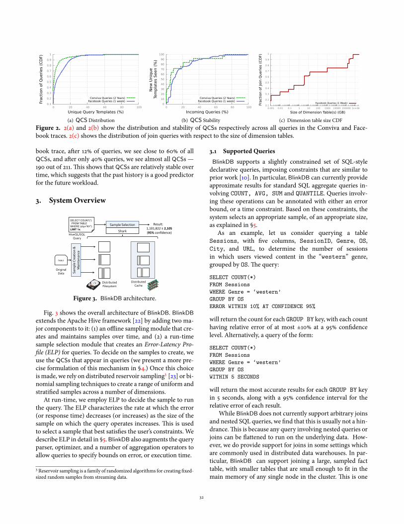
To empirically test the validity of the predictable QCS modelwe analyze a trace of 18, 096 queries from 30 days of queriesfrom Conviva and a trace of 69, 438 queries constituting arandom, but representative, fraction of 7 days’ workload fromFacebook to determine the frequency of QCSs.Fig. 2(a) shows the distribution of QCSs across all queries

for bothworkloads. Surprisingly, over 90%of queries are cov-ered by 10% and 20% of uniqueQCSs in the traces fromCon-viva and Facebook respectively. Only 182 unique QCSs coverall queries in the Conviva trace and 455 uniqueQCSs span allthe queries in the Facebook trace. Furthermore, if we removethe QCSs that appear in less than 10 queries, we end up withonly 108 and 211 QCSs covering 17, 437 queries and 68, 785queries from Conviva and Facebook workloads, respectively.�is suggests that, for real-world production workloads,QCSs represent an excellent model of future queries.Fig. 2(b) shows the number of unique QCSs versus the

queries arriving in the system. We de�ne unique QCSs asQCSs that appear in more than 10 queries. For the Con-viva trace, a�er only 6% of queries we already see close to60% of all QCSs, and a�er 30% of queries have arrived, wesee almost all QCSs — 100 out of 108. Similarly, for the Face-

2 Typically, these blocks are 64 − 1024 MB in size.

31

0.1

0.2

0.3

0.4

0.5

0.6

0.7

0.8

0.9

1

0 20 40 60 80 100

Fract

ion o

f Q

ueri

es

(CD

F)

Unique Query Templates (%)

Conviva Queries (2 Years)Facebook Queries (1 week)

(a) QCS Distribution

0

10

20

30

40

50

60

70

80

90

100

0 20 40 60 80 100

New

Uniq

ue

Tem

pla

tes

Seen (

%)

Incoming Queries (%)

Conviva Queries (2 Years)Facebook Queries (1 week)

(b) QCS Stability

0.1

0.2

0.3

0.4

0.5

0.6

0.7

0.8

0.9

1

0.001 0.01 0.1 1 10 100 1000 10000 100000 1e+06

Fract

ion o

f Jo

in Q

ueri

es

(CD

F)

Size of Dimension Table(s) (GB)

Facebook Queries (1 Week)

(c) Dimension table size CDFFigure 2. 2(a) and 2(b) show the distribution and stability of QCSs respectively across all queries in the Conviva and Face-book traces. 2(c) shows the distribution of join queries with respect to the size of dimension tables.

book trace, a�er 12% of queries, we see close to 60% of allQCSs, and a�er only 40% queries, we see almost all QCSs —190 out of 211.�is shows that QCSs are relatively stable overtime, which suggests that the past history is a good predictorfor the future workload.

3. System Overview

Sample'Selection'

TABLE'

Distributed'Cache'

Distributed'Filesystem'

Original''Data'

Shark'

'SELECT COUNT(*)! FROM TABLE!WHERE (city=“NY”)!LIMIT 1s;!

HiveQL/SQL'Query'

Result:(1,101,822(±(2,105&&(95%(confidence)(

Sample'Crea

tion'&'

Mainten

ance

'

Figure 3. BlinkDB architecture.

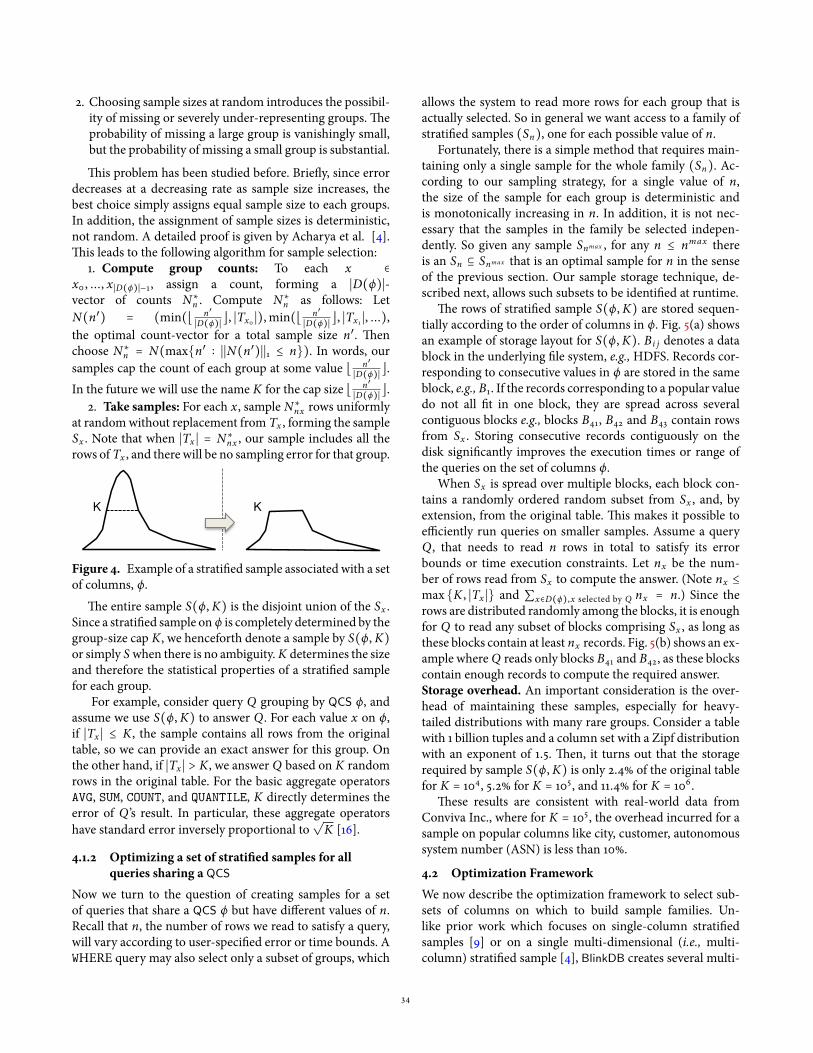
Fig. 3 shows the overall architecture of BlinkDB. BlinkDBextends the Apache Hive framework [22] by adding two ma-jor components to it: (1) an o�ine sampling module that cre-ates and maintains samples over time, and (2) a run-timesample selection module that creates an Error-Latency Pro-�le (ELP) for queries. To decide on the samples to create, weuse the QCSs that appear in queries (we present a more pre-cise formulation of this mechanism in §4.) Once this choiceis made, we rely on distributed reservoir sampling3 [23] or bi-nomial sampling techniques to create a range of uniform andstrati�ed samples across a number of dimensions.At run-time, we employ ELP to decide the sample to run

the query.�e ELP characterizes the rate at which the error(or response time) decreases (or increases) as the size of thesample on which the query operates increases.�is is usedto select a sample that best satis�es the user’s constraints. Wedescribe ELP in detail in §5.BlinkDB also augments the queryparser, optimizer, and a number of aggregation operators toallow queries to specify bounds on error, or execution time.

3 Reservoir sampling is a family of randomized algorithms for creating �xed-sized random samples from streaming data.

3.1 Supported Queries

BlinkDB supports a slightly constrained set of SQL-styledeclarative queries, imposing constraints that are similar toprior work [10]. In particular, BlinkDB can currently provideapproximate results for standard SQL aggregate queries in-volving COUNT, AVG, SUM and QUANTILE. Queries involv-ing these operations can be annotated with either an errorbound, or a time constraint. Based on these constraints, thesystem selects an appropriate sample, of an appropriate size,as explained in §5.As an example, let us consider querying a table

Sessions, with �ve columns, SessionID, Genre, OS,City, and URL, to determine the number of sessionsin which users viewed content in the “western” genre,grouped by OS.�e query:

SELECT COUNT(*)

FROM Sessions

WHERE Genre = ‘western’

GROUP BY OS

ERROR WITHIN 10% AT CONFIDENCE 95%

will return the count for each GROUP BY key, with each counthaving relative error of at most ±10% at a 95% con�dencelevel. Alternatively, a query of the form:

SELECT COUNT(*)

FROM Sessions

WHERE Genre = ‘western’

GROUP BY OS

WITHIN 5 SECONDS

will return the most accurate results for each GROUP BY keyin 5 seconds, along with a 95% con�dence interval for therelative error of each result.While BlinkDB does not currently support arbitrary joins

and nested SQL queries, we �nd that this is usually not a hin-drance.�is is because any query involving nested queries orjoins can be �attened to run on the underlying data. How-ever, we do provide support for joins in some settings whichare commonly used in distributed data warehouses. In par-ticular, BlinkDB can support joining a large, sampled facttable, with smaller tables that are small enough to �t in themain memory of any single node in the cluster.�is is one

32

Notation DescriptionT fact (original) tableQ a queryt a time bound for query Qe an error bound for query Qn the estimated number of rows that can be

accessed in time tϕ the QCS for Q, a set of columns in Tx a ∣ϕ∣-tuple of values for a column set ϕ, for

example (Berkeley, CA) for ϕ =(City, State)D(ϕ) the set of all unique x-values for ϕ in TTx , Sx the rows in T (or a subset S ⊆ T) having the

values x on ϕ (ϕ is implicit)S(ϕ,K) strati�ed sample associated with ϕ, where

frequency of every group x in ϕ is capped by K∆(ϕ,M) the number of groups in T under ϕ having

size less thanM — a measure of sparsity of T

Table 1. Notation in §4.1

of the most commonly used form of joins in distributed datawarehouses. For instance, Fig. 2(c) shows the distribution ofthe size of dimension tables (i.e., all tables except the largest)across all queries in a week’s trace from Facebook. We ob-serve that 70%of the queries involve dimension tables that areless than 100 GB in size.�ese dimension tables can be easilycached in the cluster memory, assuming a cluster consistingof hundreds or thousands of nodes, where each node has atleast 32 GB RAM. It would also be straightforward to extendBlinkDB to deal with foreign key joins between two sampledtables (or a self join on one sampled table) where both ta-bles have a strati�ed sample on the set of columns used forjoins. We are also working on extending our query model tosupport more general queries, speci�cally focusing on morecomplicated user de�ned functions, and on nested queries.

4. Sample CreationBlinkDB creates a set of samples to accurately and quickly an-swer queries. In this section, we describe the sample creationprocess in detail. First, in §4.1, we discuss the creation of astrati�ed sample on a given set of columns. We show how aquery’s accuracy and response time depends on the availabil-ity of strati�ed samples for that query, and evaluate the stor-age requirements of our strati�ed sampling strategy for vari-ous data distributions. Strati�ed samples are useful, but carrystorage costs, so we can only build a limited number of them.In §4.2 we formulate and solve an optimization problem todecide on the sets of columns on which we build samples.

4.1 Strati�ed Samples

In this section, we describe our techniques for constructing asample to target queries using a given QCS. Table 1 containsthe notation used in the rest of this section.Queries that do not �lter or group data (for example, a SUM

over an entire table) o�en produce accurate answers whenrun on uniform samples. However, uniform sampling o�en

does notworkwell for a queries on �ltered or grouped subsetsof the table. When members of a particular subset are rare,a larger sample will be required to produce high-con�denceestimates on that subset. A uniform sample may not containany members of the subset at all, leading to a missing row inthe �nal output of the query.�e standard approach to solv-ing this problem is strati�ed sampling [16], which ensures thatrare subgroups are su�ciently represented. Next, we describethe use of strati�ed sampling in BlinkDB.

4.1.1 Optimizing a strati�ed sample for a single query

First, consider the smaller problem of optimizing a strati�edsample for a single query. We are given a query Q specifyinga table T , a QCS ϕ, and either a response time bound t oran error bound e. A time bound t determines the maximumsample size on which we can operate, n; n is also the opti-mal sample size, since larger samples produce better statisti-cal results. Similarly, given an error bound e, it is possible tocalculate the minimum sample size that will satisfy the errorbound, and any larger sample would be suboptimal becauseit would take longer than necessary. In general n is monoton-ically increasing in t (or monotonically decreasing in e) butwill also depend on Q and on the resources available in thecluster to processQ.Wewill show later in §5 howwe estimaten at runtime using an Error-Latency Pro�le.Among the rows in T , let D(ϕ) be the set of unique values

x on the columns in ϕ. For each value x there is a set of rowsin T having that value, Tx = {r ∶ r ∈ T and r takes values xon columns ϕ}. We will say that there are ∣D(ϕ)∣ “groups” Txof rows in T under ϕ. We would like to compute an aggregatevalue for each Tx (for example, a SUM). Since that is expensive,instead we will choose a sample S ⊆ T with ∣S∣ = n rows.For each group Tx there is a corresponding sample groupSx ⊆ S that is a subset of Tx , which will be used instead ofTx to calculate an aggregate. �e aggregate calculation foreach Sx will be subject to error that will depend on its size.�e best sampling strategy will minimize some measure ofthe expected error of the aggregate across all the Sx , such asthe worst expected error or the average expected error.A standard approach is uniform sampling — sampling n

rows from T with equal probability. It is important to un-derstand why this is an imperfect solution for queries thatcompute aggregates on groups. A uniform random sampleallocates a random number of rows to each group.�e sizeof sample group Sx has a hypergeometric distribution with ndraws, population size ∣T ∣, and ∣Tx ∣ possibilities for the groupto be drawn.�e expected size of Sx is n ∣Tx ∣

∣T ∣ , which is propor-tional to ∣Tx ∣. For small ∣Tx ∣, there is a chance that ∣Sx ∣ is verysmall or even zero, so the uniform sampling scheme canmisssome groups just by chance.�ere are 2 things going wrong:

1. �e sample size assigned to a group depends on its size inT . If we care about the error of each aggregate equally, itis not clear why we should assign more samples to Sx justbecause ∣Tx ∣ is larger.

33

2. Choosing sample sizes at random introduces the possibil-ity of missing or severely under-representing groups.�eprobability of missing a large group is vanishingly small,but the probability of missing a small group is substantial.

�is problem has been studied before. Brie�y, since errordecreases at a decreasing rate as sample size increases, thebest choice simply assigns equal sample size to each groups.In addition, the assignment of sample sizes is deterministic,not random. A detailed proof is given by Acharya et al. [4].�is leads to the following algorithm for sample selection:1. Compute group counts: To each x ∈

x0 , ..., x∣D(ϕ)∣−1, assign a count, forming a ∣D(ϕ)∣-vector of counts N∗

n . Compute N∗

n as follows: LetN(n′) = (min(⌊ n′

∣D(ϕ)∣ ⌋, ∣Tx0 ∣), min(⌊ n′∣D(ϕ)∣ ⌋, ∣Tx1 ∣, ...),

the optimal count-vector for a total sample size n′. �enchoose N∗

n = N(max{n′ ∶ ∣∣N(n′)∣∣1 ≤ n}). In words, oursamples cap the count of each group at some value ⌊ n′

∣D(ϕ)∣ ⌋.In the future we will use the name K for the cap size ⌊ n′

∣D(ϕ)∣ ⌋.2. Take samples: For each x, sample N∗

nx rows uniformlyat randomwithout replacement from Tx , forming the sampleSx . Note that when ∣Tx ∣ = N∗

nx , our sample includes all therows of Tx , and there will be no sampling error for that group.

V(φ) S(φ)

K K

φ

Figure 4. Example of a strati�ed sample associated with a setof columns, ϕ.

�e entire sample S(ϕ,K) is the disjoint union of the Sx .Since a strati�ed sample on ϕ is completely determined by thegroup-size cap K, we henceforth denote a sample by S(ϕ,K)or simply S when there is no ambiguity.K determines the sizeand therefore the statistical properties of a strati�ed samplefor each group.For example, consider query Q grouping by QCS ϕ, and

assume we use S(ϕ,K) to answer Q. For each value x on ϕ,if ∣Tx ∣ ≤ K, the sample contains all rows from the originaltable, so we can provide an exact answer for this group. Onthe other hand, if ∣Tx ∣ > K, we answer Q based on K randomrows in the original table. For the basic aggregate operatorsAVG, SUM, COUNT, and QUANTILE, K directly determines theerror of Q’s result. In particular, these aggregate operatorshave standard error inversely proportional to

√K [16].

4.1.2 Optimizing a set of strati�ed samples for allqueries sharing a QCS

Now we turn to the question of creating samples for a setof queries that share a QCS ϕ but have di�erent values of n.Recall that n, the number of rows we read to satisfy a query,will vary according to user-speci�ed error or time bounds. AWHERE query may also select only a subset of groups, which

allows the system to read more rows for each group that isactually selected. So in general we want access to a family ofstrati�ed samples (Sn), one for each possible value of n.Fortunately, there is a simple method that requires main-

taining only a single sample for the whole family (Sn). Ac-cording to our sampling strategy, for a single value of n,the size of the sample for each group is deterministic andis monotonically increasing in n. In addition, it is not nec-essary that the samples in the family be selected indepen-dently. So given any sample Snmax , for any n ≤ nmax thereis an Sn ⊆ Snmax that is an optimal sample for n in the senseof the previous section. Our sample storage technique, de-scribed next, allows such subsets to be identi�ed at runtime.

�e rows of strati�ed sample S(ϕ,K) are stored sequen-tially according to the order of columns in ϕ. Fig. 5(a) showsan example of storage layout for S(ϕ,K). B i j denotes a datablock in the underlying �le system, e.g., HDFS. Records cor-responding to consecutive values in ϕ are stored in the sameblock, e.g., B1. If the records corresponding to a popular valuedo not all �t in one block, they are spread across severalcontiguous blocks e.g., blocks B41, B42 and B43 contain rowsfrom Sx . Storing consecutive records contiguously on thedisk signi�cantly improves the execution times or range ofthe queries on the set of columns ϕ.When Sx is spread over multiple blocks, each block con-

tains a randomly ordered random subset from Sx , and, byextension, from the original table.�is makes it possible toe�ciently run queries on smaller samples. Assume a queryQ, that needs to read n rows in total to satisfy its errorbounds or time execution constraints. Let nx be the num-ber of rows read from Sx to compute the answer. (Note nx ≤max {K , ∣Tx ∣} and ∑x∈D(ϕ),x selected by Q nx = n.) Since therows are distributed randomly among the blocks, it is enoughfor Q to read any subset of blocks comprising Sx , as long asthese blocks contain at least nx records. Fig. 5(b) shows an ex-ample whereQ reads only blocks B41 and B42, as these blockscontain enough records to compute the required answer.Storage overhead. An important consideration is the over-head of maintaining these samples, especially for heavy-tailed distributions with many rare groups. Consider a tablewith 1 billion tuples and a column set with a Zipf distributionwith an exponent of 1.5.�en, it turns out that the storagerequired by sample S(ϕ,K) is only 2.4% of the original tablefor K = 104, 5.2% for K = 105, and 11.4% for K = 106.

�ese results are consistent with real-world data fromConviva Inc., where for K = 105, the overhead incurred for asample on popular columns like city, customer, autonomoussystem number (ASN) is less than 10%.

4.2 Optimization Framework

We now describe the optimization framework to select sub-sets of columns on which to build sample families. Un-like prior work which focuses on single-column strati�edsamples [9] or on a single multi-dimensional (i.e., multi-column) strati�ed sample [4], BlinkDB creates several multi-

34

K

B1

B21

B22

B31

B32

B33

B41

B42

B51

B52

B6 B7 B8

B43

x

(a)

K

B1

B21

B22

B31

B32

B33

B51

B52

B6 B7 B8

B43

K1 B42

B41

x

(b)Figure 5. (a) Possible storage layout for strati�ed sample S(ϕ,K).

dimensional strati�ed samples. As described above, eachstrati�ed sample can potentially be used at runtime to im-prove query accuracy and latency, especially when the orig-inal table contains small groups for a particular column set.However, each stored sample has a storage cost equal to itssize, and the number of potential samples is exponential inthe number of columns. As a result, we need to be carefulin choosing the set of column-sets on which to build strati-�ed samples.We formulate the trade-o� between storage costand query accuracy/performance as an optimization prob-lem, described next.

4.2.1 Problem Formulation

�e optimization problem takes three factors into account indetermining the sets of columns on which strati�ed samplesshould be built: the “sparsity” of the data,workload character-istics, and the storage cost of samples.

Sparsity of the data. A strati�ed sample on ϕ is useful whenthe original table T contains many small groups under ϕ.Consider aQCS ϕ in table T . Recall thatD(ϕ) denotes the setof all distinct values on columns ϕ in rows of T . We de�ne a“sparsity” function ∆(ϕ,M) as the number of groups whosesize in T is less than some numberM4:

∆(ϕ,M) = ∣{x ∈ D(ϕ) ∶ ∣Tx ∣ < M}∣Workload.A strati�ed sample is only useful when it is bene-�cial to actual queries. Under our model for queries, a queryhas a QCS q j with some (unknown) probability p j - that is,QCSs are drawn from aMultinomial (p1 , p2 , ...) distribution.�e best estimate of p j is simply the frequency of queries withQCS q j in past queries.

Storage cost. Storage is the main constraint against build-ing too many strati�ed samples, and against building strat-i�ed samples on large column sets that produce too manygroups.�erefore, we must compute the storage cost of po-tential samples and constrain total storage. To simplify theformulation, we assume a single value of K for all samples;a sample family ϕ either receives no samples or a full sam-ple with K elements of Tx for each x ∈ D(ϕ). ∣S(ϕ,K)∣ is thestorage cost (in rows) of building a strati�ed sample on a setof columns ϕ.4Appropriate values for M will be discussed later in this section. Alterna-tively, one could plug in di�erent notions of sparsity of a distribution in ourformulation.

Given these three factors de�ned above, we now introduceour optimization formulation. Let the overall storage capacitybudget (again in rows) be C. Our goal is to select β columnsets from among m possible QCSs, say ϕ i1 ,⋯, ϕ iβ , which canbest answer our queries, while satisfying:

β

∑k=1

∣S(ϕ ik ,K)∣ ≤ C

Speci�cally, inBlinkDB, wemaximize the followingmixedinteger linear program (MILP) in which j indexes over allqueries and i indexes over all possible column sets:

G =∑jp j ⋅ y j ⋅ ∆(q j ,M) (1)

subject tom∑i=1

∣S(ϕ i ,K)∣ ⋅ z i ≤ C (2)

and

∀ j ∶ y j ≤ maxi∶ϕ i⊆q j∪i∶ϕ i⊃q j

(z i min 1,∣D(ϕ i)∣∣D(q j)∣

) (3)

where 0 ≤ y j ≤ 1 and z i ∈ {0, 1} are variables.Here, z i is a binary variable determiningwhether a sample

family should be built or not, i.e., when z i = 1, we build asample family on ϕ i ; otherwise, when z i = 0, we do not.

�e goal function (1) aims to maximize the weighted sumof the coverage of the QCSs of the queries, q j . If we create astrati�ed sample S(ϕ i ,K), the coverage of this sample for q jis de�ned as the probability that a given value x of columns q jis also present among the rows of S(ϕ i ,K). If ϕ i ⊇ q j , then q jis covered exactly, but ϕ i ⊂ q j can also be useful by partiallycovering q j . At runtime, if no strati�ed sample is available thatexactly covers the QCS for a query, a partially-covering QCSmay be used instead. In particular, the uniform sample is adegenerate case with ϕ i = ∅; it is useful for many queries butless useful than more targeted strati�ed samples.Since the coverage probability is hard to compute in prac-

tice, in this paper we approximate it by y j , which is deter-mined by constraint (3).�e y j value is in [0, 1], with 0mean-ing no coverage, and 1 meaning full coverage.�e intuitionbehind (3) is that when we build a strati�ed sample on asubset of columns ϕ i ⊆ q j , i.e. when z i = 1, we have par-tially covered q j , too. We compute this coverage as the ra-tio of the number of unique values between the two sets, i.e.,

35

∣D(ϕ i)∣/∣D(q j)∣. When ϕ i ⊂ q j , this ratio, and the true cov-erage value, is at most 1.When ϕ i = q j , the number of uniquevalues in ϕ i and q j are the same, we are guaranteed to see allthe unique values of q j in the strati�ed sample over ϕ i andtherefore the coverage will be 1. When ϕ i ⊃ q j , the coverageis also 1, so we cap the ratio ∣D(ϕ i)∣/∣D(q j)∣ at 1.Finally, we need to weigh the coverage of each set of

columns by their importance: a set of columns q j is more im-portant to cover when: (i) it appears inmore queries, which isrepresented by p j , or (ii) when there are more small groupsunder q j , which is represented by ∆(q j ,M).�us, the bestsolution is when we maximize the sum of p j ⋅ y j ⋅ ∆(q j ,M)for all QCSs, as captured by our goal function (1).

�e size of this optimization problem increases exponen-tially with the number of columns in T , which looks worry-ing. However, it is possible to solve these problems in prac-tice by applying some simple optimizations, like consideringonly column sets that actually occurred in the past queries,or eliminating column sets that are unrealistically large.Finally, we must return to two important constants we

have le� in our formulation, M and K. In practice we setM = K = 100000. Our experimental results in §7 show thatthe system performs quite well on the datasets we considerusing these parameter values.

5. BlinkDB RuntimeIn this section, we provide an overview of query execution inBlinkDB and present our approach for online sample selec-tion. Given a queryQ, the goal is to select one (ormore) sam-ple(s) at run-time that meet the speci�ed time or error con-straints and then compute answers over them. Picking a sam-ple involves selecting either the uniform sample or one of thestrati�ed samples (none of which may stratify on exactly theQCS ofQ), and then possibly executing the query on a subsetof tuples from the selected sample.�e selection of a sample(i.e., uniform or strati�ed) depends on the set of columns inQ’s clauses, the selectivity of its selection predicates, and thedata placement and distribution. In turn, the size of the sam-ple subset on which we ultimately execute the query dependson Q’s time/accuracy constraints, its computation complex-ity, the physical distribution of data in the cluster, and avail-able cluster resources (i.e., empty slots) at runtime.As with traditional query processing, accurately predict-

ing the selectivity is hard, especially for complex WHERE andGROUP BY clauses.�is problem is compounded by the factthat the underlying data distribution can change with the ar-rival of new data. Accurately estimating the query responsetime is even harder, especially when the query is executed ina distributed fashion.�is is (in part) due to variations inma-chine load, network throughput, as well as a variety of non-deterministic (sometimes time-dependent) factors that cancause wide performance �uctuations.Furthermore, maintaining a large number of samples

(which are cached in memory to di�erent extents), allows

BlinkDB to generate many di�erent query plans for the samequery that may operate on di�erent samples to satisfy thesame error/response time constraints. In order to pick thebest possible plan,BlinkDB’s run-time dynamic sample selec-tion strategy involves executing the query on a small sample(i.e., a subsample) of data of one or more samples and gath-ering statistics about the query’s selectivity, complexity andthe underlying distribution of its inputs. Based on these re-sults and the available resources, BlinkDB extrapolates the re-sponse time and relative error with respect to sample sizes toconstruct an Error Latency Pro�le (ELP) of the query for eachsample, assuming di�erent subset sizes. An ELP is a heuris-tic that enables quick evaluation of di�erent query plans inBlinkDB to pick the one that can best satisfy a query’s er-ror/response time constraints. However, it should be notedthat depending on the distribution of underlying data and thecomplexity of the query, such an estimatemight not always beaccurate, in which case BlinkDBmay need to read additionaldata to meet the query’s error/response time constraints.In the rest of this section, we detail our approach to query

execution, by �rst discussing our mechanism for selecting aset of appropriate samples (§5.1), and then picking an appro-priate subset size from one of those samples by constructingthe Error Latency Pro�le for the query (§5.2). Finally, we dis-cuss how BlinkDB corrects the bias introduced by executingqueries on strati�ed samples (§5.4).

5.1 Selecting the Sample

Choosing an appropriate sample for a query primarily de-pends on the set of columns q j that occur in its WHERE and/orGROUP BY clauses and the physical distribution of data in thecluster (i.e., disk vs. memory). If BlinkDB �nds one or morestrati�ed samples on a set of columns ϕ i such that q j ⊆ ϕ i , wesimply pick the ϕ i with the smallest number of columns, andrun the query on S(ϕ i ,K). However, if there is no strati�edsample on a column set that is a superset of q j , we run Q inparallel on in-memory subsets of all samples currently main-tained by the system. �en, out of these samples we selectthose that have a high selectivity as compared to others, whereselectivity is de�ned as the ratio of (i) the number of rows se-lected by Q, to (ii) the number of rows read by Q (i.e., num-ber of rows in that sample).�e intuition behind this choiceis that the response time of Q increases with the number ofrows it reads, while the error decreases with the number ofrows Q’s WHERE/GROUP BY clause selects.5.2 Selecting the Right Sample/Size

Once a set of samples is decided, BlinkDB needs to selecta particular sample ϕ i and pick an appropriately sized sub-sample in that sample based on the query’s response timeor error constraints. We accomplish this by constructing anELP for the query.�e ELP characterizes the rate at whichthe error decreases (and the query response time increases)with increasing sample sizes, and is built simply by runningthe query on smaller samples to estimate the selectivity and

36

project latency and error for larger samples. For a distributedquery, its runtime scales with sample size, with the scalingrate depending on the exact query structure (JOINS, GROUP

BYs etc.), physical placement of its inputs and the underlyingdata distribution [7].�e variation of error (or the varianceof the estimator) primarily depends on the variance of theunderlying data distribution and the actual number of tuplesprocessed in the sample, which in turn depends on the selec-tivity of a query’s predicates.

Error Pro�le: An error pro�le is created for all queries witherror constraints. IfQ speci�es an error (e.g., standard devia-tion) constraint, the BlinkDB error pro�le tries to predict thesize of the smallest sample that satis�es Q’s error constraint.Variance and con�dence intervals for aggregate functions areestimated using standard closed-form formulas from statis-tics [16]. For all standard SQL aggregates, the variance is pro-portional to ∼ 1/n, and thus the standard deviation (or thestatistical error) is proportional to ∼ 1/

√n, where n is the

number of rows from a sample of size N that match Q’s �lterpredicates. Using this notation. the selectivity sq of the queryis the ratio n/N .Let n i ,m be the number of rows selected by Q when run-

ning on a subset m of the strati�ed sample, S(ϕ i ,K). Fur-thermore, BlinkDB estimates the query selectivity sq , samplevariance Sn (for AVG/SUM) and the input data distribution f(for Quantiles) by running the query on a number of smallsample subsets. Using these parameter estimates, we calcu-late the number of rows n = n i ,m required to meet Q’s errorconstraints using standard closed form statistical error esti-mates [16].�en, we run Q on S(ϕ i ,K) until it reads n rows.

Latency Pro�le: Similarly, a latency pro�le is created for allqueries with response time constraints. If Q speci�es a re-sponse time constraint, we select the sample on which to runQ the same way as above. Again, let S(ϕ i ,K) be the selectedsample, and let n be themaximumnumber of rows thatQ canread without exceeding its response time constraint.�en wesimply run Q until reading n rows from S(ϕ i ,K).

�e value of n depends on the physical placement of inputdata (disk vs. memory), the query structure and complexity,and the degree of parallelism (or the resources available to thequery). As a simpli�cation, BlinkDB simply predicts n by as-suming that latency scales linearly with input size, as is com-monly observed with a majority of I/O bounded queries inparallel distributed execution environments [8, 26]. To avoidnon-linearities that may arise when running on very smallin-memory samples, BlinkDB runs a few smaller samples un-til performance seems to grow linearly and then estimatesthe appropriate linear scaling constants (i.e., data processingrate(s), disk/memory I/O rates etc.) for the model.

5.3 An Example

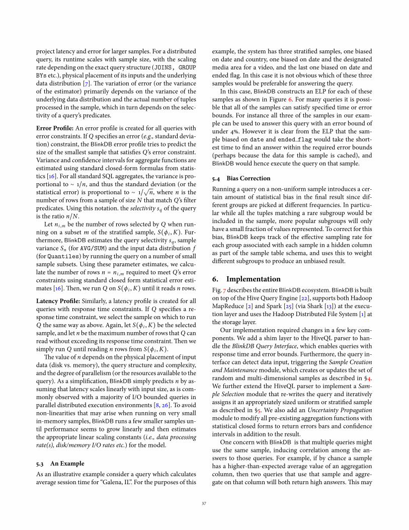
As an illustrative example consider a query which calculatesaverage session time for “Galena, IL”. For the purposes of this

example, the system has three strati�ed samples, one biasedon date and country, one biased on date and the designatedmedia area for a video, and the last one biased on date andended �ag. In this case it is not obvious which of these threesamples would be preferable for answering the query.In this case, BlinkDB constructs an ELP for each of these

samples as shown in Figure 6. For many queries it is possi-ble that all of the samples can satisfy speci�ed time or errorbounds. For instance all three of the samples in our exam-ple can be used to answer this query with an error bound ofunder 4%. However it is clear from the ELP that the sam-ple biased on date and ended flag would take the short-est time to �nd an answer within the required error bounds(perhaps because the data for this sample is cached), andBlinkDB would hence execute the query on that sample.

5.4 Bias Correction

Running a query on a non-uniform sample introduces a cer-tain amount of statistical bias in the �nal result since dif-ferent groups are picked at di�erent frequencies. In particu-lar while all the tuples matching a rare subgroup would beincluded in the sample, more popular subgroups will onlyhave a small fraction of values represented. To correct for thisbias, BlinkDB keeps track of the e�ective sampling rate foreach group associated with each sample in a hidden columnas part of the sample table schema, and uses this to weightdi�erent subgroups to produce an unbiased result.

6. ImplementationFig. 7 describes the entireBlinkDB ecosystem.BlinkDB is builton top of the Hive Query Engine [22], supports both HadoopMapReduce [2] and Spark [25] (via Shark [13]) at the execu-tion layer and uses the Hadoop Distributed File System [1] atthe storage layer.Our implementation required changes in a few key com-

ponents. We add a shim layer to the HiveQL parser to han-dle the BlinkDB Query Interface, which enables queries withresponse time and error bounds. Furthermore, the query in-terface can detect data input, triggering the Sample CreationandMaintenancemodule, which creates or updates the set ofrandom and multi-dimensional samples as described in §4.We further extend the HiveQL parser to implement a Sam-ple Selection module that re-writes the query and iterativelyassigns it an appropriately sized uniform or strati�ed sampleas described in §5. We also add an Uncertainty Propagationmodule tomodify all pre-existing aggregation functions withstatistical closed forms to return errors bars and con�denceintervals in addition to the result.One concern with BlinkDB is that multiple queries might

use the same sample, inducing correlation among the an-swers to those queries. For example, if by chance a samplehas a higher-than-expected average value of an aggregationcolumn, then two queries that use that sample and aggre-gate on that column will both return high answers.�is may

37

(a) dt, country

(b) dt, dma

(c) dt, ended flag

Figure 6. Error Latency Pro�les for a variety of samples when executing a query to calculate average session time in Galena.(a) Shows the ELP for a sample biased on date and country, (b) is the ELP for a sample biased on date and designated mediaarea (dma), and (c) is the ELP for a sample biased on date and the ended flag.

Hadoop  Distributed  File  System  (HDFS)  

Spark  

Hadoop  MapReduce  

BlinkDB  Metastore  

Hive  Query  Engine  

Shark  (Hive  on  Spark)  

Sample  Creation  and    Maintenance  

BlinkDB  Query  Interface  

Sample  Selection  Uncertainty  Propagation  

Figure 7. BlinkDB’s Implementation Stack

introduce subtle inaccuracies in analysis based on multiplequeries. By contrast, in a system that creates a new samplefor each query, a high answer for the �rst query is not pre-dictive of a high answer for the second. However, as we havealready discussed in §2, precomputing samples is essential forperformance in a distributed setting. We address correlationamong query results by periodically replacing the set of sam-ples used.BlinkDB runs a low priority background taskwhichperiodically (typically, daily) samples from the original data,creating new samples which are then used by the system.An additional concern is that the workload might change

over time, and the sample types we compute are no longer“optimal”. To alleviate this concern, BlinkDB keeps track ofstatistical properties of the underlying data (e.g., varianceand percentiles) and periodically runs the sample creationmodule described in §4 to re-compute these properties anddecide whether the set of samples needs to be changed. Toreduce the churn caused due to this process, an operator canset a parameter to control the percentage of sample that canbe changed at any single time.In BlinkDB, uniform samples are generally created in a

few hundred seconds.�is is because the time taken to createthem only depends on the disk/memory bandwidth and thedegree of parallelism. On the other hand, creating strati�edsamples on a set of columns takes anywhere between a 5 −30 minutes depending on the number of unique values tostratify on, which decides the number of reducers and theamount of data shu�ed.

7. EvaluationIn this section, we evaluate BlinkDB’s performance on a 100node EC2 cluster using a workload from Conviva Inc. and

the well-known TPC-H benchmark [3]. First, we compareBlinkDB to query execution on full-sized datasets to demon-strate how even a small trade-o� in the accuracy of �nalanswers can result in orders-of-magnitude improvements inquery response times. Second, we evaluate the accuracy andconvergence properties of our optimal multi-dimensionalstrati�ed-sampling approach against both random samplingand single-column strati�ed-sampling approaches.�ird, weevaluate the e�ectiveness of our cost models and error pro-jections at meeting the user’s accuracy/response time re-quirements. Finally, we demonstrateBlinkDB’s ability to scalegracefully with increasing cluster size.

7.1 Evaluation Setting

�e Conviva and the TPC-H datasets were 17 TB and 1 TB(i.e., a scale factor of 1000) in size, respectively, andwere bothstored across 100 Amazon EC2 extra large instances (eachwith 8 CPU cores (2.66 GHz), 68.4 GB of RAM, and 800GB of disk). �e cluster was con�gured to utilize 75 TB ofdistributed disk storage and 6 TB of distributed RAM cache.

Conviva Workload. �e Conviva data represents informa-tion about video streams viewed by Internet users. We usequery traces from their SQL-based ad-hoc querying systemwhich is used for problem diagnosis and data analytics on alog of media accesses by Conviva users.�ese access logs are1.7 TB in size and constitute a small fraction of data collectedacross 30 days. Based on their underlying data distribution,we generated a 17 TB dataset for our experiments andpartitioned it across 100 nodes.�e data consists of a singlelarge fact table with 104 columns, such as customer ID,

city, media URL, genre, date, time, user OS,

browser type, request response time, etc. �e 17TB dataset has about 5.5 billion rows and shares all the keycharacteristics of real-world production workloads observedat Facebook Inc. and Microso� Corp. [7].

�e raw query log consists of 19, 296 queries, from whichwe selected di�erent subsets for each of our experiments.We ran our optimization function on a sample of about 200queries representing 42 query column sets. We repeated theexperiments with di�erent storage budgets for the strati�edsamples– 50%, 100%, and 200%. A storage budget of x% in-

38

0 20 40 60 80

100 120 140 160 180 200

50% 100% 200%

Act

ual S

tora

ge C

ost

(%

)

Storage Budget (%)

[dt jointimems][objectid jointimems]

[dt dma]

[country endedflag][dt country]

[other columns]

(a) Biased Samples (Conviva)

0 20 40 60 80

100 120 140 160 180 200

50% 100% 200%

Act

ual S

tora

ge C

ost

(%

)

Storage Budget (%)

[orderkey suppkey][commitdt receiptdt]

[quantity]

[discount][shipmode]

[other columns]

(b) Biased Samples (TPC-H)

1

10

100

1000

10000

100000

2.5TB 7.5TB

Query

Serv

ice T

ime

(seco

nd

s)

Input Data Size (TB)

HiveHive on Spark (without caching)

Hive on Spark (with caching)BlinkDB (1% relative error)

(c) BlinkDB Vs. No SamplingFigure 8. 8(a) and 8(b) show the relative sizes of the set of strati�ed sample(s) created for 50%, 100% and 200% storage budgeton Conviva and TPC-H workloads respectively. 8(c) compares the response times (in log scale) incurred by Hive (on Hadoop),Shark (Hive on Spark) – both with and without input data caching, and BlinkDB, on simple aggregation.

dicates that the cumulative size of all the samples will not ex-ceed x

100 times the original data. So, for example, a budgetof 100% indicates that the total size of all the samples shouldbe less than or equal to the original data. Fig. 8(a) shows theset of samples that were selected by our optimization prob-lem for the storage budgets of 50%, 100% and 200% respec-tively, along with their cumulative storage costs. Note thateach strati�ed sample has a di�erent size due to variable num-ber of distinct keys in the table. For these samples, the valueof K for strati�ed sampling is set to 100, 000.

TPC-HWorkload.We also ran a smaller number of experi-ments using the TPC-H workload to demonstrate the gener-ality of our results, with respect to a standard benchmark. Allthe TPC-H experiments ran on the same 100 node cluster, on1 TB of data (i.e., a scale factor of 1000).�e 22 benchmarkqueries in TPC-H were mapped to 6 unique query columnsets. Fig. 8(b) shows the set of sample selected by our opti-mization problem for the storage budgets of 50%, 100% and200%, along with their cumulative storage costs. Unless oth-erwise speci�ed, all the experiments in this paper are donewith a 50% additional storage budget (i.e., samples could useadditional storage of up to 50% of the original data size).

7.2 BlinkDB vs. No Sampling

We �rst compare the performance of BlinkDB versus frame-works that execute queries on complete data. In this exper-iment, we ran on two subsets of the Conviva data, with 7.5TB and 2.5 TB respectively, spread across 100 machines. Wechose these two subsets to demonstrate some key aspects ofthe interaction between data-parallel frameworks and mod-ern clusters with high-memory servers.While the smaller 2.5TB dataset can be be completely cached in memory, datasetslarger than 6 TB in size have to be (at least partially) spilled todisk. To demonstrate the signi�cance of sampling even for thesimplest analytical queries, we ran a simple query that com-puted average of user session timeswith a �ltering predicateon the date column (dt) and a GROUP BY on the city column.We compared the response time of the full (accurate) execu-tion of this query on Hive [22] on Hadoop MapReduce [2],Hive on Spark (called Shark [13]) – both with and withoutcaching, against its (approximate) execution onBlinkDBwitha 1% error bound for each GROUP BY key at 95% con�dence.

We ran this query on both data sizes (i.e., corresponding to5 and 15 days worth of logs, respectively) on the aforemen-tioned 100-node cluster. We repeated each query 10 times,and report the average response time in Figure 8(c). Note thatthe Y axis is log scale. In all cases, BlinkDB signi�cantly out-performs its counterparts (by a factor of 10 − 200×), becauseit is able to read far less data to compute a fairly accurate an-swer. For both data sizes, BlinkDB returned the answers in afew seconds as compared to thousands of seconds for others.In the 2.5 TB run, Shark’s caching capabilities help consider-ably, bringing the query runtime down to about 112 seconds.However, with 7.5 TB of data, a considerable portion of datais spilled to disk and the overall query response time is con-siderably longer.

7.3 Multi-Dimensional Strati�ed Sampling

Next, we ran a set of experiments to evaluate the error (§7.3.1)and convergence (§7.3.2) properties of our optimal multi-dimensional strati�ed-sampling approach against both sim-ple random sampling, and one-dimensional strati�ed sam-pling (i.e., strati�ed samples over a single column). For theseexperiments we constructed three sets of samples on bothConviva and TPC-H data with a 50% storage constraint:1. Uniform Samples. A sample containing 50% of the en-

tire data, chosen uniformly at random.2. Single-Dimensional Strati�ed Samples.�e column

to stratify on was chosen using the same optimization frame-work, restricted so a sample is strati�ed on exactly 1 column.3. Multi-Dimensional Strati�ed Samples. �e sets of

columns to stratify on were chosen using BlinkDB’s opti-mization framework (§4.2), restricted so that samples couldbe strati�ed on no more than 3 columns (considering fouror more column combinations caused our optimizer to takemore than a minute to complete).

7.3.1 Error Properties

In order to illustrate the advantages of ourmulti-dimensionalstrati�ed sampling strategy, we compared the average statis-tical error at 95% con�dence while running a query for 10seconds over the three sets of samples, all of which were con-strained to be of the same size.

39

1

2

3

4

5

6

7

8

9

10

QCS1(16)

QCS2(10)

QCS3(1)

QCS4(12)

QCS5(1)

Sta

tist

ical Err

or

(%)

Unique QCS

Uniform SamplesSingle ColumnMulti-Column

(a) Error Comparison (Conviva)

2

3

4

5

6

7

8

9

10

11

QCS1(4)

QCS2(6)

QCS3(3)

QCS4(7)

QCS5(1)

QCS6(1)

Sta

tist

ical Err

or

(%)

Unique QCS

Uniform SamplesSingle ColumnMulti-Column

(b) Error Comparison (TPC-H)

0.1

1

10

100

1000

10000

0 5 10 15 20 25 30 35

Tim

e (

seco

nds)

Statistical Error (%)

Uniform SamplesSingle ColumnMulti-Column

(c) Error Convergence (Conviva)Figure 9. 9(a) and 9(b) compare the average statistical error perQCSwhen running a query with �xed time budget of 10 secondsfor various sets of samples. 9(c) compares the rates of error convergence with respect to time for various sets of samples.

For our evaluation using Conviva’s data we used a set of 40of the most popular queries (with 5 unique QCSs) and 17 TBof uncompressed data on 100 nodes. We ran a similar set ofexperiments on the standard TPC-H queries (with 6 uniqueQCSs).�e queries we chose were on the l ineitem table, andwere modi�ed to conform with HiveQL syntax.In Figures 9(a), and 9(b), we report the average statisti-

cal error in the results of each of these queries when theyran on the aforementioned sets of samples.�e queries arebinned according to the set(s) of columns in their GROUP BY,WHERE and HAVING clauses (i.e., their QCSs) and the num-bers in brackets indicate the number of queries which liein each bin. Based on the storage constraints, BlinkDB’s op-timization framework had samples strati�ed on QCS1 andQCS2 for Conviva data and samples strati�ed on QCS1,QCS2 and QCS4 for TPC-H data. For common QCSs,multi-dimensional samples produce smaller statistical errorsthan either one-dimensional or random samples.�e opti-mization framework attempts to minimize expected error,rather than per-query errors, and therefore for some speci�cQCS single-dimensional strati�ed samples behave better thanmulti-dimensional samples. Overall, however, our optimiza-tion framework signi�cantly improves performance versussingle column samples.

7.3.2 Convergence Properties

We also ran experiments to demonstrate the convergenceproperties of multi-dimensional strati�ed samples used byBlinkDB. We use the same set of three samples as §7.3, takenover 17 TB of Conviva data. Over this data, we ran multiplequeries to calculate average session timeFor a particular ISP’s customers in 5 US Cities and deter-

mined the latency for achieving a particular error boundwith95% con�dence. Results from this experiment (Figure 9(c))show that error bars from running queries over multi-dimensional samples converge orders-of-magnitude fasterthan random sampling (i.e.,Hadoop Online [11, 19]), and aresigni�cantly faster to converge than single-dimensional strat-i�ed samples.

7.4 Time/Accuracy Guarantees

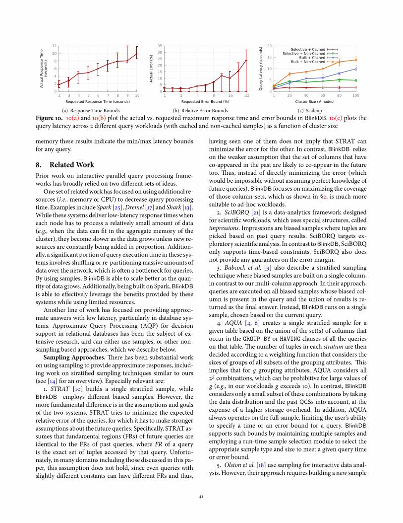
In this set of experiments, we evaluateBlinkDB’s e�ectivenessat meeting di�erent time/error bounds requested by the user.

To test time-bounded queries, we picked a sample of 20 Con-viva queries, and ran each of them 10 times, with amaximumtime bound from 1 to 10 seconds. Figure 10(a) shows the re-sults run on the same 17 TB data set, where each bar repre-sents the minimum, maximum and average response timesof the 20 queries, averaged over 10 runs. From these resultswe can see that BlinkDB is able to accurately select a sampleto satisfy a target response time.Figure 10(b) shows results from the same set of queries,

also on the 17 TB data set, evaluating our ability tomeet spec-i�ed error constraints. In this case, we varied the requestedmaximumerror bound from2% to 32% .�e bars again repre-sent the minimum, maximum and average errors across dif-ferent runs of the queries. Note that the measured error isalmost always at or less than the requested error. However,as we increase the error bound, the measured error becomescloser to the bound.�is is because at higher error rates thesample size is quite small and error bounds are wider.

7.5 Scaling Up

Finally, in order to evaluate the scalability properties ofBlinkDB as a function of cluster size, we created 2 di�erentsets of query workload suites consisting of 40 unique Con-viva queries each.�e �rst set (marked as sel ective) consistsof highly selective queries – i.e., those queries that only oper-ate on a small fraction of input data.�ese queries occur fre-quently in production workloads and consist of one or morehighly selective WHERE clauses.�e second set (marked asbulk) consists of those queries that are intended to crunchhuge amounts of data. While the former set’s input is gener-ally striped across a small number of machines, the latter setof queries generally runs on data stored on a large numberof machines, incurring a higher communication cost. Fig-ure 10(c) plots the query latency for each of these workloadsas a function of cluster size. Each query operates on 100n GBof data (where n is the cluster size). So for a 10 node clus-ter, each query operates on 1 TB of data and for a 100 nodecluster each query operates on around 10 TB of data. Fur-ther, for each workload suite, we evaluate the query latencyfor the case when the required samples are completely cachedin RAM or when they are stored entirely on disk. Since in re-ality any sample will likely partially reside both on disk and in

40

0

2

4

6

8

10

12

2 3 4 5 6 7 8 9 10

Act

ual R

esp

onse

Tim

e(s

eco

nds)

Requested Response Time (seconds)

(a) Response Time Bounds

0

5

10

15

20

25

30

35

1 2 4 8 16 32

Act

ual Err

or

(%)

Requested Error Bound (%)

(b) Relative Error Bounds

0

5

10

15

20

1 20 40 60 80 100

Query

Late

ncy

(se

conds)

Cluster Size (# nodes)

Selective + CachedSelective + Non-Cached

Bulk + CachedBulk + Non-Cached

(c) ScaleupFigure 10. 10(a) and 10(b) plot the actual vs. requested maximum response time and error bounds in BlinkDB. 10(c) plots thequery latency across 2 di�erent query workloads (with cached and non-cached samples) as a function of cluster size

memory these results indicate the min/max latency boundsfor any query.

8. RelatedWorkPrior work on interactive parallel query processing frame-works has broadly relied on two di�erent sets of ideas.One set of relatedwork has focused on using additional re-

sources (i.e.,memory or CPU) to decrease query processingtime. Examples include Spark [25],Dremel [17] and Shark [13].While these systems deliver low-latency response timeswheneach node has to process a relatively small amount of data(e.g., when the data can �t in the aggregate memory of thecluster), they become slower as the data grows unless new re-sources are constantly being added in proportion. Addition-ally, a signi�cant portion of query execution time in these sys-tems involves shu�ing or re-partitioningmassive amounts ofdata over the network, which is o�en a bottleneck for queries.By using samples, BlinkDB is able to scale better as the quan-tity of data grows. Additionally, being built on Spark,BlinkDBis able to e�ectively leverage the bene�ts provided by thesesystems while using limited resources.Another line of work has focused on providing approxi-

mate answers with low latency, particularly in database sys-tems. Approximate Query Processing (AQP) for decisionsupport in relational databases has been the subject of ex-tensive research, and can either use samples, or other non-sampling based approaches, which we describe below.

Sampling Approaches. �ere has been substantial workon using sampling to provide approximate responses, includ-ing work on strati�ed sampling techniques similar to ours(see [14] for an overview). Especially relevant are:1. STRAT [10] builds a single strati�ed sample, while

BlinkDB employs di�erent biased samples. However, themore fundamental di�erence is in the assumptions and goalsof the two systems. STRAT tries to minimize the expectedrelative error of the queries, for which it has to make strongerassumptions about the future queries. Speci�cally, STRAT as-sumes that fundamental regions (FRs) of future queries areidentical to the FRs of past queries, where FR of a queryis the exact set of tuples accessed by that query. Unfortu-nately, inmany domains including those discussed in this pa-per, this assumption does not hold, since even queries withslightly di�erent constants can have di�erent FRs and thus,

having seen one of them does not imply that STRAT canminimize the error for the other. In contrast, BlinkDB relieson the weaker assumption that the set of columns that haveco-appeared in the past are likely to co-appear in the futuretoo. �us, instead of directly minimizing the error (whichwould be impossible without assuming perfect knowledge offuture queries), BlinkDB focuses onmaximizing the coverageof those column-sets, which as shown in §2, is much moresuitable to ad-hoc workloads.2. SciBORQ [21] is a data-analytics framework designed

for scienti�c workloads, which uses special structures, calledimpressions. Impressions are biased samples where tuples arepicked based on past query results. SciBORQ targets ex-ploratory scienti�c analysis. In contrast toBlinkDB, SciBORQonly supports time-based constraints. SciBORQ also doesnot provide any guarantees on the error margin.3. Babcock et al. [9] also describe a strati�ed sampling

technique where biased samples are built on a single column,in contrast to our multi-column approach. In their approach,queries are executed on all biased samples whose biased col-umn is present in the query and the union of results is re-turned as the �nal answer. Instead, BlinkDB runs on a singlesample, chosen based on the current query.4. AQUA [4, 6] creates a single strati�ed sample for a

given table based on the union of the set(s) of columns thatoccur in the GROUP BY or HAVING clauses of all the querieson that table.�e number of tuples in each stratum are thendecided according to a weighting function that considers thesizes of groups of all subsets of the grouping attributes. �isimplies that for g grouping attributes, AQUA considers all2g combinations, which can be prohibitive for large values ofg (e.g., in our workloads g exceeds 10). In contrast, BlinkDBconsiders only a small subset of these combinations by takingthe data distribution and the past QCSs into account, at theexpense of a higher storage overhead. In addition, AQUAalways operates on the full sample, limiting the user’s abilityto specify a time or an error bound for a query. BlinkDBsupports such bounds by maintaining multiple samples andemploying a run-time sample selection module to select theappropriate sample type and size to meet a given query timeor error bound.5. Olston et al. [18] use sampling for interactive data anal-

ysis. However, their approach requires building a new sample

41

for each query template, while BlinkDB shares strati�ed sam-ples across column-sets.�is both reduces our storage over-head, and allows us to e�ectively answer queries for whichtemplates are not known a priori.

Online Aggregation.Online Aggregation (OLA) [15] andits successors [11, 19] proposed the idea of providing approx-imate answers which are constantly re�ned during query ex-ecution. It provides users with an interface to stop executiononce they are satis�ed with the current accuracy. As com-monly implemented, the main disadvantage of OLA systemsis that they stream data in a random order, which imposesa signi�cant overhead in terms of I/O. Naturally, these ap-proaches cannot exploit the workload characteristics in op-timizing the query execution. However, in principle, tech-niques like online aggregation could be added to BlinkDB,to make it continuously re�ne the values of aggregates; suchtechniques are largely orthogonal to our ideas of optimallyselecting pre-computed, strati�ed samples.

Materialized Views, Data Cubes, Wavelets, Synopses,Sketches, Histograms. �ere has been a great deal of workon “synopses” (e.g., wavelets, histograms, sketches, etc.) andlossless summaries (e.g. materialized views, data cubes). Ingeneral, these techniques are tightly tied to speci�c classes ofqueries. For instance, Vitter andWang [24] useHaar waveletsto encode a data cube without reading the least signi�cantbits of SUM/COUNT aggregates in a �at query5, but it is notclear how to use the same encoding to answer joins, sub-queries, or other complex expressions.�us, these techniquesare most applicable6 when future queries are known in ad-vance (modulo constants or other minor details). Nonethe-less, these techniques are orthogonal toBlinkDB, as one coulduse di�erent wavelets and synopses for common queries andresort to strati�ed sampling when faced with ad-hoc queriesthat cannot be supported by the current set of synopses.For instance, the join-synopsis [5] can be incorporated intoBlinkDB whereby any join query involving multiple tableswould be conceptually rewritten as a query on a single joinsynopsis relation.�us, implementing such synopsis along-side the current set of strati�ed samples in BlinkDBmay im-prove the performance for certain cases. Incorporating thestorage requirement of such synopses into our optimizationformulation makes an interesting line of future work.

9. ConclusionIn this paper, we presented BlinkDB, a parallel, sampling-based approximate query engine that provides support forad-hoc queries with error and response time constraints.BlinkDB is based on two key ideas: (i) a multi-dimensionalsampling strategy that builds and maintains a variety of sam-ples, and (ii) a run-time dynamic sample selection strategythat uses parts of a sample to estimate query selectivity and

5A SQL statement without any nested sub-queries.6Also, note that materialized views can be still too large for real-time pro-cessing.

chooses the best samples for satisfying query constraints.Evaluation results on real data sets and on deployments ofup to 100 nodes demonstrate the e�ectiveness of BlinkDB athandling a variety of queries with diverse error and time con-straints, allowing us to answer a range of queries within 2 sec-onds on 17 TB of data with 90-98% accuracy.

AcknowledgementsWeare indebted to our shepherdKimKeeton for her invaluable feedback andsuggestions that greatly improved this work. We are also grateful to SurajitChaudhuri, Michael Franklin, Phil Gibbons, Joe Hellerstein, and membersof the UC Berkeley AMP Lab for their detailed comments on the dra� andinsightful discussions on this topic.�is research is supported in part byNSFCISE Expeditions award CCF-1139158, the DARPA XData Award FA8750-12-2-0331, and gi�s from Qualcomm, Amazon Web Services, Google, SAP,Blue Goji, Cisco, Clearstory Data, Cloudera, Ericsson, Facebook, GeneralElectric, Hortonworks, Huawei, Intel, Microso�, NetApp, Oracle, Quanta,Samsung, Splunk, VMware and Yahoo!.

References[1] Apache Hadoop Distributed File System. http://hadoop.apache.org/

hdfs/.[2] Apache Hadoop Mapreduce Project. http://hadoop.apache.org/

mapreduce/.[3] TPC-H Query Processing Benchmarks. http://www.tpc.org/tpch/.[4] S. Acharya, P. B. Gibbons, and V. Poosala. Congressional samples for

approximate answering of group-by queries. In ACM SIGMOD, May 2000.[5] S. Acharya, P. B. Gibbons, V. Poosala, and S. Ramaswamy. Join synopsesfor approximate query answering. In ACM SIGMOD, June 1999.

[6] S. Acharya, P. B. Gibbons, V. Poosala, and S. Ramaswamy. The Aquaapproximate query answering system. ACM SIGMOD Record, 28(2), 1999.

[7] S. Agarwal, S. Kandula, N. Bruno, M.-C. Wu, I. Stoica, and J. Zhou. Re-optimizing Data Parallel Computing. In NSDI, 2012.

[8] G. Ananthanarayanan, S. Kandula, A. G. Greenberg, et al. Reining in theoutliers in map-reduce clusters using mantri. InOSDI, pages 265–278, 2010.

[9] B. Babcock, S. Chaudhuri, and G. Das. Dynamic sample selection forapproximate query processing. In VLDB, 2003.

[10] S. Chaudhuri, G. Das, and V. Narasayya. Optimized stratified sampling forapproximate query processing. TODS, 2007.

[11] T. Condie, N. Conway, P. Alvaro, J. M. Hellerstein, K. Elmeleegy, andR. Sears. Mapreduce online. In NSDI, 2010.

[12] G. Cormode. Sketch techniques for massive data. In Synposes for MassiveData: Samples, Histograms, Wavelets and Sketches. 2011.

[13] C. Engle, A. Lupher, R. Xin, M. Zaharia, et al. Shark: Fast Data AnalysisUsing Coarse-grained Distributed Memory. In SIGMOD, 2012.

[14] M. Garofalakis and P. Gibbons. Approximate query processing: Taming theterabytes. In VLDB, 2001. Tutorial.

[15] J. M. Hellerstein, P. J. Haas, and H. J. Wang. Online aggregation. InSIGMOD, 1997.

[16] S. Lohr. Sampling: design and analysis. Thomson, 2009.[17] S. Melnik, A. Gubarev, J. J. Long, G. Romer, S. Shivakumar, M. Tolton, and

T. Vassilakis. Dremel: interactive analysis of web-scale datasets. Commun.ACM, 54:114–123, June 2011.

[18] C. Olston, E. Bortnikov, K. Elmeleegy, F. Junqueira, and B. Reed. Interactiveanalysis of web-scale data. In CIDR, 2009.

[19] N. Pansare, V. R. Borkar, C. Jermaine, and T. Condie. Online Aggregationfor Large MapReduce Jobs. PVLDB, 4(11):1135–1145, 2011.

[20] C. Sapia. Promise: Predicting query behavior to enable predictive cachingstrategies for olap systems. DaWaK, pages 224–233. Springer-Verlag, 2000.

[21] L. Sidirourgos, M. L. Kersten, and P. A. Boncz. SciBORQ: Scientific datamanagement with Bounds On Runtime and Quality. In CIDR’11, 2011.

[22] A. Thusoo, J. S. Sarma, N. Jain, et al. Hive: a warehousing solution over amap-reduce framework. PVLDB, 2(2), 2009.

[23] S. Tirthapura and D. Woodruff. Optimal random sampling from dis-tributed streams revisited. Distributed Computing, pages 283–297, 2011.

[24] J. S. Vitter and M. Wang. Approximate computation of multidimensionalaggregates of sparse data using wavelets. SIGMOD, 1999.

[25] M. Zaharia et al. Resilient distributed datasets: A fault-tolerant abstractionfor in-memory cluster computing. In NSDI, 2012.

[26] M. Zaharia, A. Konwinski, A. D. Joseph, et al. Improving MapReducePerformance in Heterogeneous Environments. In OSDI, 2008.

42