BLIND DECONVOLUTION OF TIMELY CORRELATED SOURCES BY GRADIENT
20
Image Processing & Communications, vol.9, no.1, pp.33-52 33 BLIND DECONVOLUTION OF TIMELY CORRELATED SOURCES BY GRADIENT DESCENT SEARCH WlodzimierzKasprzak Warsaw University of Technology Institute of Control and Computation Engineering ul. Nowowiejska 15-19, PL - 00-665 Warsaw POLAND E-mail: [email protected] Abstract. In multichannel blind decon- volution (MBD) the goal is to calculate possibly scaled and delayed estimates of source signals from their convoluted mix- tures, using approximate knowledge of the source characteristics only. Nearly all of the solutions to MBD proposed so far re- quire from source signals to be pair-wise statistically independent and to be timely not correlated. In practice, this can only be satisfied by specific synthetic signals. In this paper we describe how to modify gradient-based iterative algorithms in or- der to perform the MBD task on timely correlated sources. Implementation issues are discussed and specific tests on synthetic and real 2-D images are documented. Key words. Blind source deconvolu- tion, gradient descent search, speech and image processing, unsupervised learning. 1 Introduction In speech and image recognition systems (which are based on the pattern recognition theory) [DUD73] the first processing step is to pre- process the sensor data in such a way, that the useful original source patterns are extracted without noise and disruption [GON87]. The applied methods give satisfactory results if the characteristics of disruption or source character- istics are properly predicted. But methods are needed, that can automatically adjust to the sensor signal [NIE90]. One possible way of seek- ing general solutions to source extraction lies in the increase of sensors (e.g. microphones or camera views) and the processing of a combined sensor signals (containing given pattern) at the same time. Instead of a single scalar sample we analyse vec- tor samples in a multi-dimensional space. There exist well-known methods of low-level vector sig- nal processing, which perform transformation of the representation space [WID85, CIA02]: • decorrelation in Cartesian space, • PCA, PSA - principal component (or sub- space) analysis; • ICA - independent component analysis. The decorrelation process is usually a prelimi-
Transcript of BLIND DECONVOLUTION OF TIMELY CORRELATED SOURCES BY GRADIENT
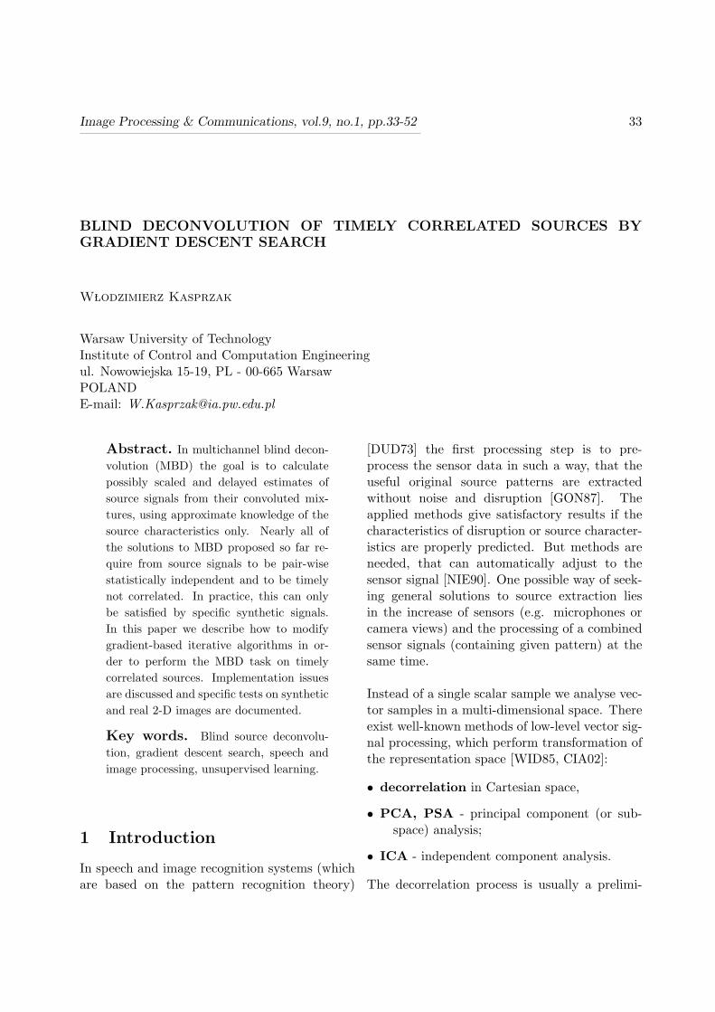
Image Processing & Communications, vol.9, no.1, pp.33-52 33
BLIND DECONVOLUTION OF TIMELY CORRELATED SOURCES BYGRADIENT DESCENT SEARCH
W lodzimierz Kasprzak
Warsaw University of TechnologyInstitute of Control and Computation Engineeringul. Nowowiejska 15-19, PL - 00-665 WarsawPOLANDE-mail: [email protected]
Abstract. In multichannel blind decon-volution (MBD) the goal is to calculatepossibly scaled and delayed estimates ofsource signals from their convoluted mix-tures, using approximate knowledge of thesource characteristics only. Nearly all ofthe solutions to MBD proposed so far re-quire from source signals to be pair-wisestatistically independent and to be timelynot correlated. In practice, this can onlybe satisfied by specific synthetic signals.In this paper we describe how to modifygradient-based iterative algorithms in or-der to perform the MBD task on timelycorrelated sources. Implementation issuesare discussed and specific tests on syntheticand real 2-D images are documented.
Key words. Blind source deconvolu-tion, gradient descent search, speech andimage processing, unsupervised learning.
1 Introduction
In speech and image recognition systems (whichare based on the pattern recognition theory)
[DUD73] the first processing step is to pre-process the sensor data in such a way, that theuseful original source patterns are extractedwithout noise and disruption [GON87]. Theapplied methods give satisfactory results if thecharacteristics of disruption or source character-istics are properly predicted. But methods areneeded, that can automatically adjust to thesensor signal [NIE90]. One possible way of seek-ing general solutions to source extraction liesin the increase of sensors (e.g. microphones orcamera views) and the processing of a combinedsensor signals (containing given pattern) at thesame time.
Instead of a single scalar sample we analyse vec-tor samples in a multi-dimensional space. Thereexist well-known methods of low-level vector sig-nal processing, which perform transformation ofthe representation space [WID85, CIA02]:
• decorrelation in Cartesian space,
• PCA, PSA - principal component (or sub-space) analysis;
• ICA - independent component analysis.
The decorrelation process is usually a prelimi-
34 W. Kasprzak
nary step for some ICA algorithms, whereas thePCA and PSA are inherently linked with signalcompression. In the context of source extractionthey are applied for noise cancellation (noisecorresponds to minor components) or orderedsequential source extraction - after a previouswhitening of the sensor signals.
One of approaches to the ICA constitutesadaptive methods of blind source separation(BSS) [HYV96, KAR97, KAS97, CIA02].They are applied to instantaneous mixtures ofsources. An extension of BSS for convolvedmixtures (mixtures in space and time) is calledBSD (blind source deconvolution) [AMA97,CIA02, HUA96]. In multichannel blind de-convolution (MBD) the goal is to calculatepossibly scaled and delayed estimates of sourcesignals from their convoluted mixtures, usingapproximate knowledge of the source char-acteristics only. Nearly all of the solutionsto MBD proposed so far require from sourcesignals to be pair-wise statistically independentand timely not correlated. In practice, thiscan only be satisfied by specific synthetic signals.
In this paper we first describe different iterativeupdate rules that can perform the MBD task.Then we discuss how to modify the updaterules in order to adapt to the self-correlationof sources. Implementation issues are discussedand specific tests on synthetic and real 2-Dimages are documented.
The paper is organised into following five mainsections. In section 2 the role of blind signal pro-cessing techniques is discussed. In section 3 thetheoretical MBD problem is introduced. Then,in section 4, the class of search-based meth-ods is described, and three specific search algo-rithms are reviewed, that can be implemented aslearning algorithms of artificial neural networks.The tests on different signal and image data aredocumented in section 5. The conclusions aredrawn in final section.
2 The role of MBD techniques
The main application fields of the blind sepa-ration/deconvolution techniques can be groupedaccording to the nature of the signal, i.e. a 1-Dsignal or a 2-D image. In the processing of 1-Dsignals we distinguish:
• Bio-medical applications: the extraction ofnervous signals in muscles and inner organs[KAR97].
• Speech processing the extraction of selectedspeaker in the ”cocktail party” problem[CIA02].
• Seismology the extraction of signals originat-ing in different earth layers.
• General data mining in different fields (e.g. aprospective application might be the sepa-ration of economic processes in overall eco-nomic data).
The pre-processing of 2-D images may include:
• The extraction of sparse binary images[PAJ96] (e.g. images of documents) (Fig. 1).
• Contrast strengthening of smoothed images inselected regions [CIA02].
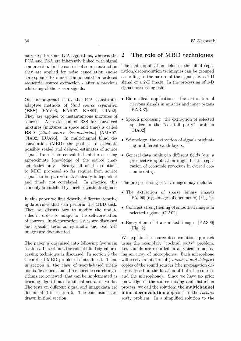
• Encryption of transmitted images [KAS96](Fig. 2).
We explain the source deconvolution approachusing the exemplary ”cocktail party” problem.Let sounds are recorded in a typical room us-ing an array of microphones. Each microphonewill receive a mixture of (convolved and delayed)copies of the sound sources (the propagation de-lay is based on the location of both the sourcesand the microphone). Since we have no priorknowledge of the source mixing and distortionprocess, we call the solution: the multichannelblind deconvolution approach to the cocktailparty problem. In a simplified solution to the
Image Processing & Communications, vol.9, no.1, pp.33-52 35
Figure 1: Blind extraction of three sparse sources (binary images) from their two mixtures.
cocktail party problem - in blind source sep-aration (BSS) we make the fundamental as-sumption that the signals are mixed together in-stantaneously, meaning that all of the signalsare time-aligned so that they enter the sensorssimultaneously without any delays.
3 The MBD problem
3.1 BSS and MBD
The multichannel blind source deconvolutionproblem (MBD) [AMA98, CIA02, HUA96,SAB98] can be considered as a natural exten-sion of the instantaneous blind source sepa-ration problem (BSS). An m-dimensional vec-tor of sensor signals (in discrete time): x(k) =[x1(k), . . . , xm(k)]T at time k, is assumed to beproduced from an n-dimensional vector of sourcesignals s(k) = [s1(k), . . . , sn(k)]T (m > n), byusing the mixture model:
x(k) =∞∑
p=−∞Hps(k−p) = Hp∗s(k) = H(z)s(k)(1)
where Hp is an (m× n) matrix of mixing coeffi-cients at lag p :
H(z) =∞∑
p=−∞Hpz
−p (2)
H(z) is a matrix transfer function. z−1 is thedelay operator defined by: z−p[si(k)] = si(k−p).
The goal of MBD is to calculate possibly scaledand delayed estimates of the source signals fromthe received signals by using an approximateknowledge of the source signal distributions andstatistics.
Two general approaches to multichannel blinddeconvolution can be considered. The first ap-proach focuses on the estimation of the multi-channel impulse response sequence {Hp} fromthe sensor signals x(k) [HUA96] and it can becalled blind identification or equalisation. In thesecond approach, on tries to estimate the directsources by a generalisation of the blind sourceseparation approach [AMA97, CIA02].
3.2 A feed-forward model for MBD
Consider a feed-forward model that estimatesthe source signals directly by using a truncatedversion of a doubly infinite multichannel equal-izer:
y(k) =∞∑
p=−∞Wp(k)x(k − p) = Wp(k) ∗ x(k)
= W(z, k)[x(k)] (3)
where y(k) = [y1(k), . . . , yn(k)]T is an n-dimensional vector of outputs,W(k) = {Wp(k) | −∞ ≤ p ≤ ∞} is a sequenceof matrices (of size n × m) at time k, and the
36 W. Kasprzak
Figure 2: Encryption of transmitted images: only the friendly receiver knows the two cover images[KAS96].
matrix transfer function is
W(z, k) =∞∑
p=−∞Wp(k)z−p (4)
In the standard BSD approach we use the neuralnetwork models for BSS but the synaptic weightsare generalised to finite-size dynamic filters(e.g. FIR), i.e. each synaptic weight:
Wij(z, k) =L∑
p=0
wijp(k)z−p (5)
is described by a finite-duration impulse re-sponse (FIR) filter at time k.
Then the goal of MBD-search is to adjustW(z; k) such that the global system is:
limk→∞
G(z, k) = W(z, k)H(z) = P0D(z) (6)
Where P0 is an n×n permutation matrix, D(z)is an n× n diagonal matrix whose (i; i)-th entryis ciz
−4i, ci is a scalar factor, and 4i is aninteger delay.
General requirements of the MBD theory are:
1. Each source has to be temporally indepen-dent, identically distributed.
2. Sources should be drawn from non-Gaussiandistributions.
3. The number of sensors is equal or greaterthan the number of independent sources.
4. The convoluting filters have no common ze-roes.
5. The convoluting filters have no zeroes on theunit circle.

Image Processing & Communications, vol.9, no.1, pp.33-52 37
The definitions of decorrelation and indepen-dence are given next. Let us consider two ran-dom variables x(t) and y(t). The following con-dition holds for decorrelated signals:
E{x · y} = E{x} · E{y} (7)
If E{x · y} = 0 then the signals are also ortho-gonal. The independence condition is defined as:
pxy(x, y) = px(x) · py(y) (8)
where pxy, px, py are pdf’s of appropriatedistributions xy, x and y.The decorrelation condition is weaker thanindependence, i.e. if x and y are independentthen they are also decorrelated.
The generalized decorrelation can be defined as:
E{f(x) · g(y)} = E{f(x)} · E{g(y)} (9)
for arbitrary non-linearitys f(.) and g(.).
Yet another, general definition of independenceis:
E{xp · yq} = E{xp} · E{yq} (10)
The ICA algorithms force all the statistical cross-moments to zero, making the output signals sta-tistically independent.
4 The gradient search methodsfor MBD
4.1 Gradient based optimisation
Two well-known iterative optimisation methodsare the stochastic gradient (or gradientdescent) method and the quasi-Newtonconvergence method [DUD73].
In gradient descent search the basic task is todefine a criterion J(W(z, k)), which obtains its
minimum for some Wopt if this Wopt is theseeked optimum solution.
The gradient descent search
1. Start with some initial point W(z, k = 0) inthe multi-dimensional parameter space.
2. Obtain the gradient value ∇J(W(z, k)).
3. Compute the value W(z, k + 1) by movingfrom W(z, k) along the gradient descent, i.e.along - ∇J(W(z, k)):
W(z, k+1) = W(z, k))−η(k)∇J(W(z, k))(11)
where η(k) is a positive-valued step scalingcoefficient.
4. Test the stability of parameters, i.e. if|W(z, k + 1)−W(z, k)| < θ (threshold).
Quasi-Newton searchAn alternative solution to gradient descentsearch is a direct minimisation of the series ex-pansion of J(W) by its first- and second-orderderivatives:
J(W) ≈ J(W(z, k)) +∇JT (W −W(z, k)) +
+12(W −W(z, k))TD(k)(W −W(z, k)) (12)
where D(k) is the Laplasjan computed at pointW(z, k).
The minimisation of J(W) appears if:
W(z, k+1) = W(z, k)−D(k)−1∇J(W(z, k))(13)
Obviously the matrix D(k) need not to besingular.
Both standard approaches suffer from practicalimplications. The stochastic gradient showsslow convergence if statistical correlation be-tween signals appear in the parameter update

38 W. Kasprzak
process. The quasi- Newton methods are oftenof heavy computational complexity and sufferfrom numerical problems.
The natural gradient search
The natural gradient search (as proposed byAmari [AMA96]) is a modified gradient descentsearch, where the standard search direction ismodified according to some local Riemannianmetric of the (weight) parameter space. Thisnew direction is invariant to the statistical rela-tionships between the model parameters, and ithas a convenient form for the MBD task:
∇JN (W(z, k)) =
= ∇J(W(z, k))WT (z−l, k)W(z, k) (14)
Gradient methods for detection of functionextremes in BSS / MBD
Let us assume a cost function E{J(W)}, depen-dent on parameters W. The most popular costminimisation approach (in many applications)uses the steepest descent form. Additionally forsolving the BSS and MBD problems another twogradient approaches were developed recentlythe natural gradient descent and the dualnatural gradient descent.
1. Steepest descent approach:
W(l + 1) = W(l)− η(l)∂E{J(W)}
∂W(15)
or its stochastic version (in which the ex-pected value is replaced by a single observa-tion):
W(k + 1) = W(k)− η(k)∂J(W(k))
∂W(k)(16)
2. Natural gradient descent approach
The natural gradient was developed in-dependently by: Amari et al. (whichgave a theoretical justification by using theRiemannian space notation) [AMA97], Ci-chocki et al. (which proposed an algorithmjustified by computer simulations) [CIC94]and Cardoso and Laheld (that introducedthe relative gradient) [CAR96]:
W(l + 1) = W(l)−
−η(l)∂E{J(W)}
∂WWT (l)W(l) (17)
or its stochastic version:
W(k + 1) = W(k)−
−η(k)∂J(W(k))
∂W(k)WT (k)W(k) (18)
3. Dual natural gradient descent approach.
This approach was introduced by Attick andRedlich:
W(l + 1) = W(l)−
−η(l)W(l)[∂E{J(W)}
∂W]TW(l) (19)
or its stochastic version:
W(k + 1) = W(k)−
−η(k)W(k)[∂J(W(k))
∂W(k)]TW(k) (20)
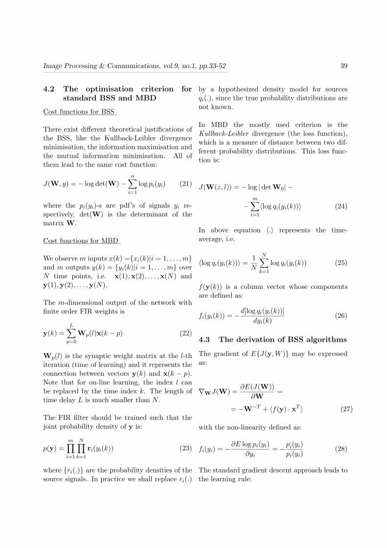
Image Processing & Communications, vol.9, no.1, pp.33-52 39
4.2 The optimisation criterion forstandard BSS and MBD
Cost functions for BSS
There exist different theoretical justifications ofthe BSS, like the Kullback-Leibler divergenceminimisation, the information maximisation andthe mutual information minimisation. All ofthem lead to the same cost function:
J(W, y) = − log det(W)−n∑
i=1
log pi(yi) (21)
where the pi(yi)-s are pdf’s of signals yi re-spectively, det(W) is the determinant of thematrix W.
Cost functions for MBD
We observe m inputs x(k) ={xi(k)|i = 1, . . . , m}and m outputs y(k) = {yi(k)|i = 1, . . . ,m} overN time points, i.e. x(1),x(2), . . . ,x(N) andy(1),y(2), . . . ,y(N).
The m-dimensional output of the network withfinite order FIR weights is
y(k) =L∑
p=0
Wp(l)x(k − p) (22)
Wp(l) is the synaptic weight matrix at the l-thiteration (time of learning) and it represents theconnection between vectors y(k) and x(k − p).Note that for on-line learning, the index l canbe replaced by the time index k. The length oftime delay L is much smaller than N .
The FIR filter should be trained such that thejoint probability density of y is:
p(y) =m∏
i=1
N∏
k=1
ri(yi(k)) (23)
where {ri(.)} are the probability densities of thesource signals. In practice we shall replace ri(.)
by a hypothesized density model for sourcesqi(.), since the true probability distributions arenot known.
In MBD the mostly used criterion is theKullback-Leibler divergence (the loss function),which is a measure of distance between two dif-ferent probability distributions. This loss func-tion is:
J(W(z, l)) = − log | detW0| −
−m∑
i=1
〈log qi(yi(k))〉 (24)
In above equation 〈.〉 represents the time-average, i.e.
〈log qi(yi(k))〉 =1N
N∑
k=1
log qi(yi(k)) (25)
f(y(k)) is a column vector whose componentsare defined as:
fi(yi(k)) = −d[log qi(yi(k))]dyi(k)
(26)
4.3 The derivation of BSS algorithms
The gradient of E{J(y,W )} may be expressedas:
∇WJ(W) =∂E(J(W))
∂W=
= −W−T + 〈f(y) · xT 〉 (27)
with the non-linearity defined as:
fi(yi) = −∂E log pi(yi)∂yi
= −p,i(yi)
pi(yi)(28)
The standard gradient descent approach leads tothe learning rule:
40 W. Kasprzak
4W(k) = −η(k)∂J(W(k))
∂W(k)=
= η(k)[W−T (k)− f(y(k)) · xT (k)] (29)
The observations of low convergence speed andthe inversion of matrix W in each iteration cycleare serious drawbacks of this standard learningrule. An initial whitening of the sensor signalscould be computed in order to speed up theconvergence of the separation rule.
Applying the natural gradient approach we mayderive the learning rule for BSS:
4W(t) = −η(t)∂E{(W(t))}
∂W(t)·WT (t) ·W(t) =
= η(t)[I− 〈f(y(t)) · yT (t)〉]W(t) (30)
By using a stochastic approximation of the av-eraging process we obtain the on-line adaptivealgorithm:
4W(k) = −η(k)bI− f(y(k)) · yT (k)cW(k)(31)
Applying the dual natural gradient descent rulewe obtain:
4W(t) = −η(t)W(t)[∂E{J(W(t))}
∂W(t)]T ·W(t) =
= η(t)[I− 〈y(t) · g(yT (t))〉]W(t) (32)
or its stochastic approximation:
4W(k) = η(k)bI− y(k) · g(yT (k))cW(k) (33)
These two natural gradient-based learning rulescan be combined together to one general, flexiblelearning rule [CIA02]:
4W(k) = η(k)bI−f(y(k)) ·g(yT (k))cW(k)(34)
4.4 Derivation of learning rules forMBD
The standard Bussgang method applies the gra-dient descent search, which gives the followingweight update (learning) rule:
Wp(k + 1) = Wp(k) + η(k)f(y(k))xT (k − p)
for lag p = 0, . . . , L (35)
In their first attempt to MBD Amari et al.[AMA97] derived the following update rule forMBD:
Wp(k + 1) = Wp(k) +
+η(k)[Wp(k)− f(y(k)) · uTp (k − p)] (36)
in which delayed cross filters are used:
up(k) =L∑
p=0
WTp (k) · y(k + p) (37)
The number of weight matrices is in practicelimited to some finite range: p = 0, . . . , L .
In a more elaborated attempt, while using thenatural gradient search, Cichocki and Amarihave obtained the following weight update(learning) rule for MBD [CIA02]:
4Wp = −ηp∑
q=0
∂J(W(z))∂Xq
Wp−q =
= ηp∑
q=0
(∂0qI− 〈f(y(k))yT (k − q)〉)Wp−q (38)
for p = 0, 1, . . . , L, where η is the learning rate.The term (∂0qI) denotes, that:
∂0qI =
{I for q = p0 for q 6= p
(39)
Image Processing & Communications, vol.9, no.1, pp.33-52 41
In particular the learning rule for W0 is :
4W0 = η(I− 〈f(y(k) · yT (k)〉) ·W0 (40)
The selection of appropriate function f(y) de-pends on the sign of the kurtosis, which is a 4-thorder statistical moment:
κ4(x) = m4 − 3m22 (41)
One can choose, for example, f(y) = y3 , for sub-Gaussian sources (with negative kurtosis) andf(y) = tanh(γy) (γ > 2), for super-Gaussiansignals (with positive kurtosis).
4.5 The modified natural-gradient up-date rule
The update rule (38) converges to the equilib-rium point, described by the two following equa-tions:
E{〈f(yi(k)) · yi(k)〉} = 1, ∀i (42)
and
E{〈f(yi(k)) · yi(k − p)〉} = 0, ∀i(p = 1, 2, . . . , L− 1) (43)
In other words, the deconvolution system,if succeeded, then it produces statisticallyindependent signals of timely non-correlatedstructure.
In practice, for most natural signals or images,both goals can only approximately be achieved,as the natural signals are pair-wise not fully inde-pendent and they also have not a correlation-freetime structure. To deal with natural signals, weneed to know their temporal structure. Probablyfor most signal categories this can only approx-imately be known. Hence, a vector of ”gener-alized correlation” coefficients is assumed to beavailable to the weight update rule:
Λp =E{〈f(x(k)) · x(k − p)〉}
E{〈f(x(k)) · x(k)〉} (44)
(p = 0, 1, 2, . . . , L− 1)
From above coefficients we form an appropriateset of diagonal matrices:
Γp =
Λp 0 . . . 00 Λp . . . 00 . . . Λp 00 0 . . . Λp
(45)
(p = 0, 1, 2, . . . , L− 1)
The modification of update rule (4.28) takes theform:
4Wp(k) =
= η(k)p∑
q=0
[Γq − f(y(k)) · yT (k − q))]Wp−q(k)(46)
5 Experimental results
5.1 Practical issues
Usually the initial step value should be selectedappropriately to the variance of input signals.We observed that the best learning results wereachieved for a descending step size. Usually, thechoice of the initial weight values affects the ini-tial convergence of the search process. Obviouslythe weight matrices need not to be zero-valued.We selected initial values of the weights from therange 〈−0.1, 0.1〉.
5.2 Measuring the quality of outputs
For test purpose we assume that the source sig-nals are known to the observer. Hence, for eachpair (output Yi ; source Sj ) with amplitudes

42 W. Kasprzak
scaled to < −1, 1 > one computes the SNR[i, j](signal to noise ratio):
SNR[i, j] = 10 · log〈S2
i 〉MSE[i, j]
(47)
where 〈S2i 〉 is the time-average of 2-nd power of
source i (i.e. the variance) and MSE[i, j] is themean square error of approximating Sj by Yi ,i.e.
MSE[i, j] =1N
N−1∑
k=0
[Si(k)− Yj(k)]2 =
= 〈(Si − Yj)2〉 (48)
with N - number of samples in one signal.
All the individual SNR-s are combined to amatrix P = [pi,j ] with pi,j = (
√MSE[i, j])−1 .
Now a combined error index EI(P) can be com-puted for the whole separated output set relativeto the source set:
EI(P) =1m
[(n∑
i=1
m∑
j=1
p2ij
maxi(p2i,j)
)− n] +
+1n
[(m∑
j=1
n∑
i=1
p2ij
maxj(p2i,j)
)−m] (49)
The pi,j-s are entries of two normalised ver-sions of matrix P. At first, each nonzero row(i = 1, . . . , n) of P is normalised, such thatmaxi(pi,j) = 1. This allows the computation offirst part of above equation (5.3). At second, thecolumns of matrix P are normalized in a similarway and the second part of (5.3) is computed.In the ideal case of perfect separation the follow-ing appears:
• P becomes a permutation matrix.
• Only one element in each row and columnequals to unity, and all the other elementsare zero.
• EI achieves its minimum possible value equalto 0.
Without the knowledge of original sources westill are able to judge about the separation qual-ity by computing the correlation factors betweenoutputs. The normalized cross-correlation be-tween each pair of output signals si and sj is:
E{si · sj}σi · σj
(50)
During the learning process the outputs shouldget less correlated. Initially the mixture signalsare highly correlated (they are to some amountstochastically dependent).
5.3 The sources
We have applied two sets of sources: artificialbinary images and natural face images (Fig. 3).In Table 1 the results of the normalisation ofsources is documented: they all are of zero-meanand of negative kurtosis.From Table 2 it is evident that the sources arehighly self-correlated in time. Hence, we ex-pect that the standard MBD rule (38) will notwork properly on convolution mixtures of suchsources.
5.4 Some test results
In our experiments three sources (assumed tobe unknown to the deconvolution system) ( (a)the synthetic binary images or (b) the naturalface images) were convolved by using a set ofmixing matrices {Aq|q = 0, . . . , M − 1}, whereeach matrix Aq was of size: m = 3, n = 3. Inpractice we set M = 4 (see Fig. 4).
The deconvolution system consisted of threeFIR filters of order (up to) L = 8, i.e. the num-ber L of delay units were in the range from 1 to 8.
The two natural-gradient based update rulesthe original one (38) and the modified one (38)

Image Processing & Communications, vol.9, no.1, pp.33-52 43
Table 1: Cross-correlation between source pairs.
mean var κ4
Binary 1 0.0 0.9256 -1.99913Binary 2 0.0 0.8005 -1.9579Binary 3 0.0 0.8003 -1.9579
mean var κ4
Face 1 0.0 0.2790 -0.9108Face 2 0.0 0.2271 -1.4727Face 3 0.0 0.1077 -0.6037
Source I - Source J 1 2 3E{sIsJ}
σIσJ
Binary 1 1.0 0.063 0.012Binary 2 1.0 0.031Binary 3 1.0
Source I - Source J 1 2 3E{sIsJ}
σIσJ
Face 1 1.0 -0.3045 0.1719Face 2 1.0 0.1727Face 3 1.0
Table 2: Auto-correlation of sources in time (p is time delay).
E{f [si(k)]sj(k−p)}σiσj
p=0 1 2 3 4 5 6 7 8 9
Binary 1 1.0 0.924 0.853 0.783 0.712 0.641 0.568 0.494 0.420 0.345Binary 2 1.0 0.939 0.881 0.824 0.766 0.710 0.653 0.596 0.539 0.483Binary 3 1.0 0.939 0.881 0.825 0.768 0.711 0.655 0.598 0.540 0.482
E{f [si(k)]sj(k−p)}σiσj
p=0 1 2 3 4 5 6 7 8 9
Face 1 1.0 0.986 0.971 0.956 0.942 0.927 0.913 0.898 0.883 0.869Face 2 1.0 0.936 0.884 0.841 0.806 0.780 0.772 0.771 0.769 0.767Face 3 1.0 0.894 0.764 0.743 0.813 0.866 0.823 0.733 0.692 0.706
Table 3: Approximation of the auto-correlation of sources in time.
Norm. time-correlation p=0 1 2 3 4 5 6 7 8 9Binary images 1.0 0.93 0.88 0.80 0.75 0.70 0.65 0.59 0.50 0.40Face images 1.0 0.93 0.88 0.85 0.85 0.85 0.83 0.78 0.76 0.76

44 W. Kasprzak
Figure 3: Sources - three synthetic binary images or three natural images.
for timely-correlated sources were tested onthese two source sets (see Fig. 5).
The modified rule (38) requires an estimatefor timely self-correlation of sources. We haveapproximated these estimates in the sameway for all sources in given set. The appliedparameter values are given in Table 3.
The quality index EI was computed for thewhole range of deconvolving weight matricesW0 −W7 (see Table 4). The quality results be-have like expected the original rule can not copewith clearly timecorrelated sources, whereas themodified rule is able to cope with these problems.
In the first case the best results were achievedafter using only the weights W0, with additionalweights corresponding to decorrelation in time,the results are steadily degrading.
In the modified rule case an improvement of thetotal output results is observed if additional ma-trices W0 −W4 are learned. In the case of faceimages after we add even more matrices, thequality is slightly decreasing again (i.e. EI isincreasing).
Image Processing & Communications, vol.9, no.1, pp.33-52 45
Figure 4: Examples of sensor signals.
6 Conclusions
Most work in the area of blind signal processingdeals with simple, synthetic sources, whichfully satisfy the independency constraints ofthe theory. Unfortunately, natural signals arequite different they have complex distributionsand are not fully statistically independent,neither in space nor in time. This paper dealswith the blind pre-processing of natural sourcemixtures. In order better to illustrate the testresults image sources have been considered.But the results are also true for 1-D signals,e.g. speech or sound sources. We have shownhow to modify the update rules in blind source
deconvolution in order to adapt to the non-zeroauto-correlation values of sources in time.
Acknowledgments
This work was supported by the Research Cen-tre for Control and Information-Decision Tech-nology (CATID) at Warsaw University of Tech-nology, Poland.
7 Bibliography
[AMA97 ] Amari S., Douglas S.C., Cichocki A.,Yang H.Y.: Novel on-line adaptive learn-ing algorithms for blind deconvolution us-

46 W. Kasprzak
Figure 5: Examples of output signals.
ing the natural gradient approach. IEEESignal Proc. Workshop on Signal Process-ing Advances in Wireless Communications,April 1997, Paris, 107 112.
[CAR96 ] Cardoso J.F., Laheld B.: Equiv-ariant adaptive source separation, IEEETrans. on Signal Processing, vol. 44(1996),December 1996, 3017-3030.
[CIA02 ] Cichocki A., Amari S., Adaptive BlindSignal and Image Processing , John Wiley,Chichester, UK, 2002.
[CIC94 ] Cichocki A., Unbehauen R., RummertE.: Robust learning algorithm for blind sep-
aration of signals, Electronics Letters, vol.30(1994), August 1994, 1386-1387.
[DUD73 ] Duda R.O., Hart P.E. : Pattern clas-sification and scene analysis, John Wiley &Sons, New York, 1973.
[HUA96 ] Hua Y.: Fast maximum-likelihoodfor blind identification of multiple FIR chan-nels, IEEE Trans. Signal Processing, vol.44 (1996), 661 - 672.
[HYV96 ] Hyvarinen A., Oja E.: Simple neuronmodels for independent component analysis,Int. J. Neural Systems, vol. 7, 1996, 671-687.
Image Processing & Communications, vol.9, no.1, pp.33-52 47
[KAR97 ] Karhunen J., Oja E., Wang L., Vi-gario R., Joutsensalo J.: A class of neuralnetworks for independent component anal-ysis, IEEE Trans. on Neural Networks, vol.8(1997), May 1997, 486-504.
[KAS00 ] Kasprzak W.: ICA algorithms forimage restoration. Chapter 3 of the mono-graph work: Kasprzak W.: Adaptive com-putation methods in digital image sequenceanalysis. Prace Naukowe - Elektronika, Nr.127 (2000), Warsaw University of TechologyPress, Warszawa, 170 pages.
[KAS96 ] Kasprzak W., Cichocki A.: HiddenImage Separation From Incomplete ImageMixtures by Independent Component Anal-ysis, 13th Int. Conf. on Pattern Recogni-tion, ICPR’96, Proceedings. IEEE Com-puter Society Press, Los Alamitos CA, 1996,vol.II, 394-398.
[KAS97 ] Kasprzak W., Cichocki A., Amari S.:Blind Source Separation with ConvolutiveNoise Cancellation, Neural Computing andApplications, Springer Ltd., London, vol. 6(1997), 127-141.
[NIE90 ] Niemann H.: Pattern Analysis andUnderstanding, Springer, Berlin, 1990.
[PAJ96 ] Pajunen P.: An Algorithm for Bi-nary Blind Source Separation, Helsinki Uni-versity of Technology, Lab. of Computerand Information Science, Report A36, July1996.
[SAB98 ] Sabaa I.: Multichannel deconvolu-tion and separation of statistically indepen-dent signals for unknown dynamic systems.Ph.D. dissertation, Warsaw University ofTechnology, Dep. of Electrical Engineering,Warsaw, 1998.
[WID85 ] Widrow B., Stearns S.D.: Adaptivesignal processing, Prentice Hall, EnglewoodCliffs, NJ, 1985.

48 W. Kasprzak
Appendix
Matlab source code of the MBD learning process
function weights = MBDLearningProc(Signal, weightsIN, EtaIN,sensnum, ...
outnum, delay, time, maxsample, Function, LAMBDAmat)% The learning procedure for multichannel blind source deconvolution,% based on the modified (by W.Kasprzak) NG- (defined by S.Amari et al.)% -based learning (update) rule%%%%%%%%%%%%%%%%%%%%%%%%%%%%%%%%Parameters:%Signal; /* the set of mixed input signals */%weightsIN; /* the weights to be learned */%EtaIN; /* the learning rate matrix */%sensnum; /* number of sensors */%outnum; /* number of outputs */%delay; /* number of time delays - shift_signum */%time; /* maximum number of learning epochs */%maxsample; /* length of one epoch */%Function; /* the index of nonlinear function */%LAMBDAmat; /* typical (expected) high-order correlation of sources in time */%%%%%%%%%%%%%%%%%%%%%%%%%%%%%%%%%%%%%%%%%%%%%%%%%% Author: Wodzimierz Kasprzak (ICCE WUT)% Place and time: Warszawa, 15. June 2002%%%%%%%%%%%%%%%%%%%%%%%%%%%%%%%%%%%%%%%%%%%%%%%%%global BLOCKLEN; global WEIGHT_DIFF; global MINIMUM_ETAINIT;%%%%%%%%%%%%%%%%%%%%%%%I. Initialisation[m,SIGLxBLL] = size(Signal); % The size of input data
weights = weightsIN; Eta = EtaIN; ffun = zeros(1,outnum); gfun =zeros(1,outnum);
% Expected high-order correlations in timeIMAT = zeros(sensnum, sensnum, delay); for (i=1: 1: delay)
IMAT(:,:,i) = diag(LAMBDAmat(:,i)’);end
%Local variabless=0; samples=0; ss=0.0; samplestep = 0.0;
%%%%%%%%%%Parameters
Image Processing & Communications, vol.9, no.1, pp.33-52 49
p = outnum; %/* output number: the y_j output index */m = sensnum; %/* sensor number: the x_i index */mmsize = m * m ; %/* m rows and m columns, quadrat */nmsize = p * m ; %/* p rows and m columns, quadrat */N = delay; %/* number of deconvolution samples for signals and ref.noise */
% Set EtainitEtainit = zeros(1,delay); % Initial learning rate in vector formEtainit = EtaIN; % default value% or (comment it out if not used)% a subfunction if Etainit should depend on varianceEtainit = SetEtainitMBD(p, m, N, Signal, Function);
%Initialize weight matrix and store it for eventual re-startwinitmem = zeros(m,m); weightmat = zeros(m,m,N); winitmem =InitWeightsMBD(Method, p, m, N, weightsIN(:,:,1)); for (i=1: 1:delay)
weightmat(:,:,i) = winitmem / i;
Etainit(i) = Etainit(i) / i;end Eta = Etainit; weights = weightmat;
%%%%%%%%%%%%%%%%%%%%%%%%%%%%% II. Repetitive learning processsstart = 1; tstart = 1; DDsamples = 0;
for (DD = 1: 1: delay) % Main loop according to time delay indexffunmat = zeros(m, DD); %f(y) in matrx formgfunmat = zeros(m, DD); %g(y) in matrix formxk = zeros(m, DD + DD); yk = zeros(p, DD); % input and output samples
%/* Main repetition loop for a single delay index */REPEAT = 1;while (REPEAT==1)
REPEAT = 0;if (Etainit(DD) < MINIMUM_ETAINIT)
fprintf(’*Error: Etainit is to small. No learning possible !\n’);break;
endblockDDsamples = 0; % number of learned blocks of samples for current DDlambda = 1.0;OrigIndex = zeros(1,m);%/* Initialize the weight matrix with index DD */Eta(DD) = Etainit(DD);weights(:,:,DD) = weightmat(:,:,DD);
50 W. Kasprzak
%/* Store current weight modules required for convergence test */wprev = 0.0;for (k=1: 1: m)
wprev = wprev + weights(k,:,DD) * (weights(k,:,DD))’;end%/* Initialize samplestep */ss = 1.0; %/* the decay step of learning rates */samplestep = 99 / SIGLxBLL;
REPEAT = 0;samples = DDsamples;DDsamples = 0;%/* c1. Epoch loop */for (s = 1 : 1 : time)
%/* Initialize indices to the ffun, gfun memory */FBegind = 0; FEndind = 1;%/* c2. Time loop */for (t = 2 : 1 : maxsample) % delay must be <= BLOCKLEN
% We need two times DD samplesblockDDsamples = blockDDsamples + 1;baseskip = t;%/* c3. Block loop */for (l = 1 : 1 : BLOCKLEN)
baseskip = baseskip + 1; samples = samples + 1;DDsamples = DDsamples + 1;%/* Get current and delayed input samples */xk = GetMultiSample(m, DD + DD, Signal, baseskip);%/* Current output samples y(t) of network ’weights’:% D output samples */yk = ConvFForwardSample(m, p, DD, weights, xk, yk);%/* Set current activation function values: ffun, gfun */for (i=1:1:DD)
lamsum = 0.0; lam2sum = 0.0;y2 = yk(:,i) .* yk(:,i);lamsum = yk(:,i)’ * yk(:,i);y3 = y2 .* yk(:,i);lam2sum = y2’ * y2;switch(Function)case 1,
ffun = y3’; gfun = yk(:,i)’; % f(y) = y^3, g(y) = y
otherwise,[ffun, gfun] = GetCurrentFunctions(m, Function, ...
ffun’, gfun’, yk(:,i)’, y2’, y3’);end

Image Processing & Communications, vol.9, no.1, pp.33-52 51
%/* Add current function value to delay function memory */ffunmat(:, i) = ffun’;gfunmat(:, i) = gfun’;
endFEndind = FEndind + 1; % DELAY_TIME% /* Scalar Eta of steady default decay - nonadaptive */Eta(DD) = Etainit(DD) / ss;ss = ss + samplestep;
%/* c4. Deconvolution learning rule */weights(:,:,DD) = MBDNGLearningRule(l, m, p, N, DD, Eta, ...
weights, ffunmat, gfunmat, IMAT);FBegind = (FBegind + 1); % DELAY_TIME;%/* Testing the stability of weights */[REPEAT, wprev] = WeightStabilityTest(m, p, mmsize, ...
Etainit, weights(:,:,DD), wprev);if (REPEAT == 1)
Etainit(DD) = 0.4 * Etainit(DD);fprintf (’(RESTART) etainit(%d)= %.6f * (10)-3\n’, ...
DD, 1000.0 * Etainit(DD));end
if (REPEAT == 1)break;
endend %/* Closing the block loop */%/* c6. Check weight restart condition */if (REPEAT ==1)
DDsamples = 0;break;
endend %/* Closing the time loop */%/* c7. Check weight restart condition, again */if (REPEAT == 1)
DDsamples = 0;break;
end%/* c8. Modify samplestep for next epoch */samplestep = 0.4 * samplestep;
end %/* Closing the epoch loop */end %/* Closing the repeat loop */
end % Closing the DD loopreturn;%%%%%%%%%%%%%%%%%%%%%%%%%%%%%%%%%%%%%%%%%%%%%%%%%%%%%%%%%%%%%%%%%%%%%%
52 W. Kasprzak
% Subfunction: the modified NG-based update rulefunction wpD = MBDNGLearningRule(ll, n, m, N, D, eta, weights, ff,gf, lmat)% A single weight matrix with for the delay index D is updated% Author: Wodzimierz Kasprzak (ICCE WUT)% Place and time: Warszawa, 15. June 2002%%%%%%%%%%%%%%%%%%%%%%%w1n = weights(:,:,1:D); wpD = zeros(m,n);k = D; %w1 = zeros(m,n); for (q = 1: 1: k)
pq = k - q + 1;if (q == 1)
w1 = w1 + (lmat(:,:,pq) - ff(:, 1) * gf(:, pq)’) * weights(:,:,pq); %else
w1 = w1 + (lmat(:,:,pq) - ff(:, 1) * gf(:, pq)’) * weights(:,:,pq); %end
end wpD = weights(:,:,k) + eta(k) * w1; return;%%%%%%%%%%%%%%%%%%%%%%%%%%%