BLIND DECONVOLUTION AND DEBLURRING

IN IMAGE ANALYSIS

Peter Hall1 and Peihua Qiu1.2

ABSTRACT. Blind deconvolution problems arise in image analysis when both

the extent of image blur, and the true image, are unknown. If a model is availablefor at least one of these quantities then, in theory, the problem is solvable. It is

generally not solvable if neither the image nor the point-spread function, whichcontrols the extent of blur, is known parametrically. In this paper we develop

methods for solution when a model is known for the point-spread function, butthe image is assessed only nonparametrically. We assume that the image includes

sharp edges — mathematically speaking, lines of discontinuity of image brightness.However, the locations, shapes and other properties of these lines are not needed

for our algorithm. Our technique involves mathematically “focussing” the restoredimage until the edges are as sharp as possible, with sharpness being measured using

a difference-based approach. We pay special attention to the Gaussian point-spread

function. Although this context is notorious in statistical deconvolution problemson account of the difficulty of finding a usable solution, it is arguably the central,

and the most important, setting for restoring blurred images. Numerical simulation,application to a real image, and theoretical analysis demonstrate the effectiveness

of our approach.

KEYWORDS. Adaptive estimation, blur, deblurring, Gaussian blur, ill-posed

problem, image restoration, inverse problem, noise, nonparametric regression, point-spread function, regularisation, test pattern.

SHORT TITLE. Image analysis.

1Centre for Mathematics and its Applications, Australian National University, Canberra, ACT

0200, Australia. The research of Peter Hall was supported in part by an ARC grant.2

School of Statistics, University of Minnesota, 389 Ford Hall, 224 Church Street SE, Minneapolis,

MN 55455, USA. The research of Peihua Qiu was supported in part by an ARC grant, a grant from

National Security Anegency of USA, and a grant from National Science Foundation of USA.

1. INTRODUCTION

Photographic images, whether recorded by digital or analogue means, have

imperfections which prevent them from conveying the “true” scene. These degra-

dations have a variety of causes, but two types, blurring and noise, are especially

common. The removal of blur, in the presence of noise, is generally an ill-posed

deconvolution problem, the solution of which requires inversion of the blur operator

followed by a smoothing step.

Although challenging, this type of problem is quite well understood if the extent

of blur can be described in precise mathematical terms. However, there is a rapidly

increasing interest in problems where the mathematical operation of blurring is

known only approximately, for example in terms of a function which depends on

unknown parameters that have to be computed from image data. This is a blind

deconvolution problem and is, of course, significantly more challenging than its

more conventional, non-blind counterpart. See, for example, work of Kundur and

Hatzinakos (1998), Carasso (2001), Galatsanos et al. (2002), and Figueiredo and

Nowak (2003).

In this paper we suggest a new technique for double-blind deconvolution when

the point-spread function, describing the manner in which blur degrades the true

image, is available only up to unknown parameters. Our approach is of interest

because it is closely linked to the physically meaningful notion of adjusting the pa-

rameters until the image is sharpest. In contrast to some earlier methods, ours does

not require detailed information about the “true” image. Instead, we recognise that

the sort of image that would be used to determine a point-spread function would

usually be one that has relatively sharp boundaries, such as those in a photographic

test pattern. We introduce a difference-based approximation, D say, to the deriva-

tive of such an image, and observe that in the absence of error, D is mathematically

virtually identical to the integral, along all boundaries, of the squared height of

jump discontinuities in image intensity. We suggest gradually altering the inverse

of a candidate point-spread function, by steadily increasing its spread, until a place

is reached where D increases sharply from a low to a high value; and then taking

the corresponding version of the function to be the correct one.

An algorithm of this type can be implemented using a threshold argument,

as follows. Gradually increase the spread of the point-spread function until D

2

exceeds the threshold, and then stop. In operation, this technique is rather like

focusing a lens and stopping when the image is at its sharpest point, except that

the extent to which the image is blurred is determined not by eye but by the

mathematical criterion D. Moreover, in the present problem, if the degree of spread

of the candidate point-spread function is increased beyond the point where it is

exactly correct, the deblurred image becomes extremely erratic, and in fact the

value of D would be theoretically infinite if we were to go beyond the critical point-

spread parameter, were it not for the influence of noise and discretisation error.

The ideal choice of threshold is the value of the integral of the square of the

jump in intensity along edges, mentioned two paragraphs above. In some instances,

the value of this integral may be known within a range. We might take the threshold

to be toward the upper end of this range, although in theory, statistically consistent

estimators can be obtained for any value in the range; see the theorem in section 3.

More generally, experimentation with different images that have approximately the

same sort of discontinuities and noise levels as the one under investigation, and

where the point-spread function is similar but known, can assist in threshold choice.

Thus our technique avoids the need for information about the true image, by

using a mathematical description of the extent to which the image is too “soft”

through the effect of blur. However, some parametric forms of point spread func-

tions differ very little, from one parameter value to another, in terms of the effects

they have on the extent to which an image is blurred. A technique based on as-

sessing the sharpness of a test pattern cannot be expected to perform well in such

circumstances. This issue is the subject of particular discussion in Section 2, which

gives general theoretical background for our technique. For simplicity, we do not

consider the effects of noise there; this matter is taken up in mathematical detail in

Section 3. A summary of numerical properties of our method is given in Section 4.

We focus on the problem of estimating the point-spread function, rather than

the obviously related one of of image restoration, since there are a great many

approaches to solving the latter problem, and our objectives would have to narrow

if we were to treat just one of them. Moreover, there is usually intrinsic interest

in the point-spread function, not the least because knowing the nature of that

function is an important step in determining the blurring mechanism, so as to

improve performance of the imaging device.

3

There is a substantial, recent statistical literature on deconvolution problems,

including four discussion papers (Cornford et al. (2004); Johnstone et al. (2004);

Haario et al. (2004); Wolfe et al. (2004)) in a single issue of the Journal of the Royal

Statistical Society. Recent statistical, or closely related, work on blind deconvolu-

tion includes that of Gassiat and Gautherat (1999), Poskitt et al. (1999), Higdon and

Yamamoto (2001), Li and Shedden (2001), Zhang et al. (2001), Doucet et al. (2002),

Ellis (2002), May et al. (2003), Rosec et al. (2003), Sotthivirat and Fessler (2003),

Carasso (2004), Erdogmus et al. (2004), and Likas and Galatsanos (2004).

2. MODELS AND METHODOLOGY

2.1. Models for point-spread function. Denote by X(x, y) the brightness of an image

at a point (x, y) in the plane IR2. We consider the function X to be “blurred” by

a point-spread function, φθ, where θ denotes the value of an unknown (possibly

vector valued) parameter on which the point-spread function depends. The result

is the observed, blurred image

Y θ(x, y) =

∫ ∫φθ(u, v)X(x− u, y − v) du dv , (x, y) ∈ IR2 . (2.1)

(Here and below, unqualified integrals are taken over the whole real line or the

entire plane.) Importantly, in none of the work in this paper do we assume that X

is known. This is especially relevant when the image represented by X is degraded

by stochastic noise as well as by systematic blur; see Section 3 for discussion of the

case of noise.

We may view Y θ as the result φθX , say, of operating on X by the linear

transform with kernel φθ. (For economy of notation we use the same notation for

both a point-spread function and the associated linear operator.) For the most part

we assume θ is univariate. We suppose too that φθ preserves average brightness, in

the sense that for each θ,∫ ∫

φθ(x, y) dx dy = 1 . (2.2)

Examples include the Gaussian point-spread function

φθGau(x, y) =

1

2πθexp

{− 1

2

(x2 + y2

)/θ}, (x, y) ∈ IR2 . (2.3)

Although, as statisticians know from experience in errors-in-variables problems,

this type of blur is especially challenging for deconvolution, it is especially common

4

in applications of image analysis. One of the reasons is the central, canonical

role played by the Gaussian density function, which comes about in part through

arguments based on the Central Limit Theorem.

The circular-exponential point-spread function,

φθexp(x, y) =

1

2π θ2exp

{− θ−1 (x2 + y2)1/2

}, (x, y) ∈ IR2 , (2.4)

where θ > 0, is occasionally discussed in image analysis. One generalisation of φθGau

is to the circular, “stable” point-spread function,

φθsta(x, y) = θ−2

2 ψθ1

sta

{(x, y)/θ2

}, (x, y) ∈ IR2 , (2.5)

where θ = (θ1, θ2), 0 < θ1 ≤ 2, θ2 > 0, and ψθ1

sta denotes the density of a bivariate,

symmetric, stable law, with characteristic function

∫ ∫exp{−(isx+ ity)}ψθ1

sta(x, y) dx dy = exp{− (s2 + t2)θ1/2

}, (s, t) ∈ IR2 .

The Gaussian case is obtained by taking, in (2.5), θ1 = 2 and θ2 proportional to

the standard deviation.

2.2. Models for images. The type of image that is most likely to be useful for

determining a point-spread function is one that includes sharp boundaries. That

is, if we represent an image as a function, X , from the plane to the real line, then

the function should include jump discontinuities. Such functions can be thought

of as modelling the intensity of light reflected from a typical test-pattern used in

photography. Rows of lines in the test-pattern are represented mathematically

as long, narrow, closely-spaced rows of rectangular blocks, on each of which the

function takes a particular value, say 1, and off which it takes a different value,

say 0.

An example to which we pay special attention, because of its mathematical

simplicity, is the square-block test-pattern, where the image is represented as the

function

X(x, y) ={

1 if |x| ≤ 1 and |y| ≤ 10 otherwise .

(2.6)

Note, however, that we do not need to know the true image; that is, the function

X is not assumed known. Our approach supposes only that X is a function with

fault-type discontinuities; we do not require information about their location, height

or extent.

5

2.3. Effect of deblurring on discontinuities. If a function X of the type discussed

in Section 2.2 is smoothed by the operator φθ0 , producing the blurred function

Y θ0 defined at (2.1), then vertical fault-type discontinuities in X will generally be

converted to sloping surfaces in Y θ0 = φθ0X . Conversely, if we attempt to recover

the image represented by X by applying the inverse of φθ to Y θ0 , then in many

cases we should be able to determine the correct value of θ (that is, θ = θ0) by

considering which values of θ produce a function

Zθ =(φθ

)−1Y θ0 =

(φθ

)−1φθ0X (2.7)

that has had fault-type discontinuities restored to it.

Since we do not assume that the true image represented by X is known, then

we do not know where to look for the fault lines, or how to assess how high the

jump discontinuities might be. Thus, rather than make a subjective assessment of

image smoothness we require a mathematical criterion, based on differentiation or

differencing. Such an approach is discussed in the next section.

To appreciate in more detail the effect that the choice of θ has on properties

of Zθ, defined at (2.7), assume that θ is a scalar parameter and that increasing θ

increases the extent of “spread” of φθ. Examples include the Gaussian and circular-

exponential point-spread functions, at (2.3) and (2.4), respectively, and also the

circular-stable point-spread function at (2.5) if θ1 is fixed and θ = θ2 is varied, or if

θ2 is fixed and θ = θ1 is altered. In such cases, if the univariate parameter θ is too

small then applying the inverse operator, (φθ)−1, to Y θ = φθ0X , as at (2.7), will not

fully compensate for the blurring action that took X to Y θ. However, increasing

θ all the way to θ = θ0 will cause the image to “snap into focus,” and allow us to

recover X perfectly. On the other hand, increasing θ beyond θ0 will cause Zθ to

fluctuate in a highly erratic manner, especially if some noise is present. By assessing

these situations mathematically, we have an opportunity to determine the correct

value of θ.

Let φθft denote the Fourier transform of φθ:

φθft(s, t) =

1

(2π)2

∫ ∫φθ(x, y) exp{−(isx+ ity)} dx dy . (2.8)

Mathematically, the point-spread functions considered in the previous paragraph,

with θ univariate and with the exception of the circular-exponential function, all

6

have the following properties:

if 0 < θ1 < θ2 then for each C > 0, |φθ2

ft (s, t)/φθ1

ft (s, t)| is bounded above

by a constant multiple of (1 + |s| + |t|)−C , uniformly in (s, t) ∈ IR2.(2.9)

Since C in (2.9) can be chosen arbitrarily large, then the implications of (2.9) may

be expressed in words as follows: If 0 < θ1 < θ2 then the effect that φθ2 has on

dampening down high-frequency portions of the function X is exponentially greater,

as a function of those frequencies, than the effect had by φθ1 . Here we interpret “ex-

ponentially greater” as meaning “greater than any polynomial function,” although

in the examples in the previous paragraph it actually is a conventional exponential

function.

2.4. Measuring the sharpness of a blurred image. If the extent of deblurring is

too small, then the deblurred image will be relatively “soft.” In particular, if φθ

satisfies (2.9) and θ is strictly less than the correct value θ0, then, even when X

contains fault-type discontinuities, Zθ (representing our attempt at deblurring the

blurred version, Y θ0 , of X) will be differentiable. On the other hand, provided X

contains fault-type discontinuities, Zθ will fail to be differentiable if we deblur by

exactly the right amount, or if we deblur too much. These considerations suggest

that we might measure the sharpness of the deblurred image by assessing the extent

to which Zθ is differentiable.

Of course, in practice we have to do all our calculations on a discrete grid,

representing the pixel grid on which images are digitised. Therefore, we are inter-

ested in difference operators as much as we are in differentiation. The methodology

discussed below is strongly influenced by this consideration.

Let h > 0 denote a small positive quantity, let Z = Zθ represent our attempt

at restoring the function Y θ, obtained by smoothing X , and define

A(h) = (2h)−1

∫ ∫max

ω

{Z(x+ h cosω, y + h sinω)

− Z(x− h cosω, y − h sinω)}2

dx dy , (2.10)

A1(h) = (2h)−1

∫ ∫ [{Z(x+ h, y) − Z(x− h, y)}2

+ {Z(x, y + h) − Z(x, y − h)}2]dx dy . (2.11)

Clearly,

A1(h) ≤ 2A(h) , (2.12)

7

and so if discontinuities in Z were evident from the criterion A1(h), they would also

be apparent from A(h).

We show in Appendix A.1 that, if Z is smooth except for fault-type disconti-

nuities along a collection, C, of curves in the plane, and if f(s) denotes the jump

height at s ∈ C, then as h→ 0,

A(h) →∫

C

f(s)2 ds , (2.13)

the latter denoting the line integral of f2 along C. Of course, C does not need to be

a single connected curve, and need not be smooth; it may contain corners.

The limit for A1(h) is less explicit than that for A(h), but always lies between 1

and√

2 times the limit for A(h): as h→ 0,

A1(h) → α

∫

C

f(s)2 ds , (2.14)

where 1 ≤ α ≤√

2. In general, α will depend on C and f in a complex manner. To

obtain (2.13) and (2.14) in Appendix A.1 we assume that, at points away from C,

the function X is smooth, in the sense of having a bounded derivative.

Results (2.13) and (2.14) demonstrate the ability of the criteria A and A1 to

discern places in Z where brightness changes rapidly. In particular, A and A1 are

not appreciably affected by smooth parts of Z, and A(h) is asymptotically equal to

the integrated squared height of jump discontinuities.

2.5. Properties of A and A1 when applied to Zθ. Let us assume that a graph of

the surface z = X(x, y) shows a nondegenerate collection, C, of fault-type discon-

tinuities, but that X is smooth elsewhere and, in addition, is compactly supported

so that it is square-integrable on IR2. (The square-block test-pattern, for which X

is given at (2.6), is a case in point.) If we have chosen θ = θ0 exactly right in the

definition of Z = Zθ at (2.7), then Z = X , and so by (2.13) and (2.14), A(h) and

A1(h) both converge to a strictly positive constant as h→ 0.

On the other hand, if the point-spread function φθ satisfies (2.9) and if θ < θ0,

then it can be proved, using a simple argument based on Fourier transforms, that

the function Z = Zθ has infinitely many square-integrable derivatives on IR2. In

consequence, the values of A(h) and A1(h) for this Z both converge to zero as

h → 0. Therefore, the fact that we have used a value of θ that is too small can be

recognised from the property that A(h) and A1(h) are also unduly small.

8

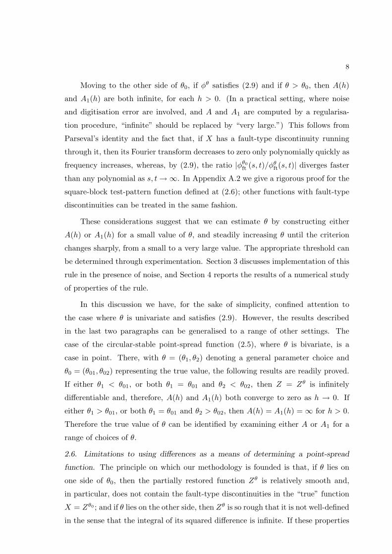
Moving to the other side of θ0, if φθ satisfies (2.9) and if θ > θ0, then A(h)

and A1(h) are both infinite, for each h > 0. (In a practical setting, where noise

and digitisation error are involved, and A and A1 are computed by a regularisa-

tion procedure, “infinite” should be replaced by “very large.”) This follows from

Parseval’s identity and the fact that, if X has a fault-type discontinuity running

through it, then its Fourier transform decreases to zero only polynomially quickly as

frequency increases, whereas, by (2.9), the ratio |φθ0

ft (s, t)/φθft(s, t)| diverges faster

than any polynomial as s, t→ ∞. In Appendix A.2 we give a rigorous proof for the

square-block test-pattern function defined at (2.6); other functions with fault-type

discontinuities can be treated in the same fashion.

These considerations suggest that we can estimate θ by constructing either

A(h) or A1(h) for a small value of θ, and steadily increasing θ until the criterion

changes sharply, from a small to a very large value. The appropriate threshold can

be determined through experimentation. Section 3 discusses implementation of this

rule in the presence of noise, and Section 4 reports the results of a numerical study

of properties of the rule.

In this discussion we have, for the sake of simplicity, confined attention to

the case where θ is univariate and satisfies (2.9). However, the results described

in the last two paragraphs can be generalised to a range of other settings. The

case of the circular-stable point-spread function (2.5), where θ is bivariate, is a

case in point. There, with θ = (θ1, θ2) denoting a general parameter choice and

θ0 = (θ01, θ02) representing the true value, the following results are readily proved.

If either θ1 < θ01, or both θ1 = θ01 and θ2 < θ02, then Z = Zθ is infinitely

differentiable and, therefore, A(h) and A1(h) both converge to zero as h → 0. If

either θ1 > θ01, or both θ1 = θ01 and θ2 > θ02, then A(h) = A1(h) = ∞ for h > 0.

Therefore the true value of θ can be identified by examining either A or A1 for a

range of choices of θ.

2.6. Limitations to using differences as a means of determining a point-spread

function. The principle on which our methodology is founded is that, if θ lies on

one side of θ0, then the partially restored function Zθ is relatively smooth and,

in particular, does not contain the fault-type discontinuities in the “true” function

X = Zθ0 ; and if θ lies on the other side, then Zθ is so rough that it is not well-defined

in the sense that the integral of its squared difference is infinite. If these properties

9

do not hold then a method based on assessing the roughness of Zθ, whether by

using the criteria A and A1 or by employing another approach, is unlikely to be

effective.

Consider, for example, the case of a point-spread function which has the prop-

erty that a fault-type discontinuity can persist in the restored function Zθ no matter

on what side of θ0 the value of θ lies. In this context the presence of a discontinuity in

Zθ cannot be used to characterise the correct choice of θ. We show in Appendix A.2

that the circular-exponential function φθexp, defined at (2.4), is of this type. This

function does not satisfy (2.9), because altering the value of θ does not have a very

large effect on the impact that smoothing has on high-frequency parts of the image.

For example, if X denotes the square-block test-pattern function defined at (2.6),

if θ0 > 0 is fixed, if Z = Zθ is defined by (2.7), and if A(h) and A1(h) are given by

(2.10) and (2.11), then no matter what the value of θ, A(h) and A1(h) converge to

strictly positive constants as h → 0. The function Zθ, given at (2.7), still contains

a fault-type discontinuity, no matter what the values of θ and θ0.

This problem is intrinsic to methodologies that use differentiation, or differ-

encing, to assess the efficacy of restoration. It is not an artifact of the particular

techniques we have chosen. If using the incorrect amount of deblurring does not

result in either marked undersmoothing (e.g. rendering a discontinuous function

smooth) or oversmoothing (making a function extremely rough, in the sense that

it is no longer square-integrable), then it is very difficult to use differentiation or

differencing as a means of determining the extent of deblurring.

3. EFFECTS OF NOISE

3.1. Main results. In practice the blurred image, represented in Section 2 by the

function Y θ0 = φθ0X , is not observed exactly. In particular, there is a degree of

noise at the level of the pixel grid. In this section we investigate the impact of that

source of error.

If noise is added to φθ0X then we need to re-define the function Y θ0 that

represents the observed image. Rather than treat pixels explicitly, we use a bivariate

form of the white-noise model:

Y θ0(x, y) =(φθ0X

)(x, y) + δ dW (x, y) , (3.1)

where W denotes a standard Wiener process in the plane. White-noise models, as

10

problems with Weiner-process noise are often called, are used in statistics as a means

of ensuring theoretical justification for methodology, while retaining the insight and

clarity that only a relatively incisive argument can provide. The equivalence of

white-noise problems to discrete-data problems is well established in a range of

settings. See, for example, Brown and Low (1996), Nussbaum (1996) and Brown et

al. (2002).

In more conventional applications of the white-noise model in statistics, involv-

ing samples of size n, the “scale” δ is taken proportional to n−1/2. In the context

of data on a pixel grid, “sample size” can be represented by the number of pixels

per unit area of the plane, N say, and δ is proportional to N−1/2. Therefore, our

asymptotic theory will be based on δ decreasing to zero.

In order to counteract the effects of noise we compute Fourier transforms in

an increasing, although compact, region that for simplicity is assumed to be the

disc Rr of radius r centred at the origin. (An alternative approach would be to use

a compactly supported stochastic process in place of W , at (3.1), but that would

arguably not be a realistic assumption.) To distinguish truncated Fourier transforms

from regular ones, we use the subscript “tft,” rather than “ft,” to indicate the

former. In particular, the truncated Fourier transform of Y θ0 , at (3.1), is

Y θ0

tft (s, t) =1

(2π)2

∫ ∫

Rr

(φθ0X

)(x, y) exp{−(isx+ ity)} dx dy

+δ

(2π)2

∫ ∫

Rr

exp{−(isx+ ity)} dW (x, y) . (3.2)

The dependence of Y θ0

tft on θ0, here and below, serves only to indicate that Y θ0

tft is

based on the actual signal Y θ0 , computed for the true value of the parameter. It does

not mean that the true parameter value has to be known in order to compute Y θ0

tft .

We “deblur” Y θ0 by dividing Y θ0

tft by φθft, treating the ratio as a Fourier trans-

form, and inverting it using a hard-thresholding approach to regularisation, obtain-

ing

V θ(x, y) =

∫ ∫Y θ0

tft (s, t)

φθft(s, t)

exp{i (sx+ ty)} I(s2 + t2 ≤ λ2

)ds dt , (3.3)

where λ > 0 denotes the threshold. If there were no noise, in particular if δ = 0

in (3.1), and if we were to take r = λ = ∞ in (3.2) and (3.3), then V θ would be

identical to Zθ defined at (2.7). When δ 6= 0, finite values of r and λ are necessary

in order to reduce the effects of noise. In such cases, the function V θ at (3.3) is

11

generally not real-valued. However, this is not a problem, since we are not interested

in V θ for its own sake, but instead in using it to construct versions of the difference

operators A(h) and A1(h).

Indeed, writing |z| for the absolute value of a complex number z, we construct

the following generalised forms of A(h) and A1(h) at (2.10) and (2.11), respectively:

Bθ(h) = (2h)−1

∫ ∫max

ω

∣∣∣V θ(x+ h cosω, y + h sinω)

− V θ(x− h cosω, y − h sinω)∣∣∣2

dx dy ,

Bθ1(h) = (2h)−1

∫ ∫ {∣∣V θ(x+ h, y) − V θ(x− h, y)∣∣2

+∣∣V θ(x, y + h) − V θ(x, y − h)

∣∣2}dx dy .

For simplicity we work only with the latter, which by Parseval’s identity is

Bθ1(h) = 2h−1 1

(2π)2

∫ ∫ ∣∣∣∣Y θ0

tft (s, t)

φθft(s, t)

∣∣∣∣2 (

sin2 sh+sin2 th)I(s2+t2 ≤ λ2

)ds dt . (3.4)

If there is no noise and we take r = λ = ∞, then Bθ1 is identical to A1 at (2.11). Note

particularly that, as indicated by (3.4), smoothing is undertaken in the frequency

rather than the spatial domain. As a result, smoothing has very little deleterious

impact on jump discontinuities or similar non-regular features of the true image.

The discussion in Section 2 suggests that simple thresholding rules, based on

the value of Bθ1(h), may be used to determine θ0. Two such rules are given below

Let C be strictly positive but otherwise arbitrary, and let θ denote either

the least value of θ for which Bθ1(h) ≥ C, or the least value of θ such that

Bθ1

1 (h) ≥ C for all θ1 ≥ θ.

(3.5)

We claim that, for a range of point-spread functions which includes those satisfying

(2.9), both algorithms in (3.5) produce statistically consistent estimators of θ0.

The convergence rate of estimators of θ0 can generally be improved by using refined

versions of those algorithms, but that will not concern us here; for simplicity we

focus only on consistency. Moreover, since the assumptions imposed on h, r and λ

will depend on choice of the parametric class of point-spread function, we reduce

the length of our treatment by considering only the Gaussian case, at (2.3). Our

method of proof is also valid for circular-stable point-spread functions, at (2.5).

12

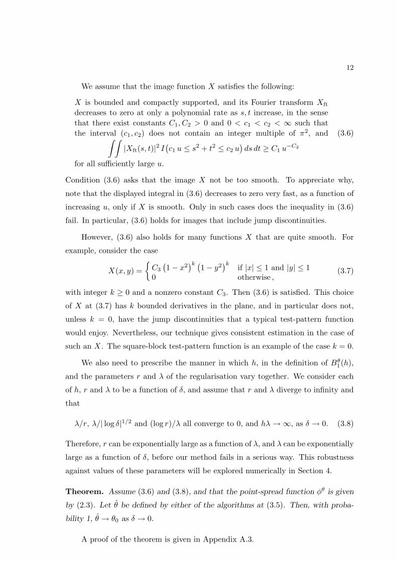
We assume that the image function X satisfies the following:

X is bounded and compactly supported, and its Fourier transform Xft

decreases to zero at only a polynomial rate as s, t increase, in the sense

that there exist constants C1, C2 > 0 and 0 < c1 < c2 < ∞ such that

the interval (c1, c2) does not contain an integer multiple of π2, and∫ ∫|Xft(s, t)|2 I

(c1 u ≤ s2 + t2 ≤ c2 u

)ds dt ≥ C1 u

−C2

for all sufficiently large u.

(3.6)

Condition (3.6) asks that the image X not be too smooth. To appreciate why,

note that the displayed integral in (3.6) decreases to zero very fast, as a function of

increasing u, only if X is smooth. Only in such cases does the inequality in (3.6)

fail. In particular, (3.6) holds for images that include jump discontinuities.

However, (3.6) also holds for many functions X that are quite smooth. For

example, consider the case

X(x, y) =

{C3

(1 − x2

)k (1 − y2

)kif |x| ≤ 1 and |y| ≤ 1

0 otherwise ,(3.7)

with integer k ≥ 0 and a nonzero constant C3. Then (3.6) is satisfied. This choice

of X at (3.7) has k bounded derivatives in the plane, and in particular does not,

unless k = 0, have the jump discontinuities that a typical test-pattern function

would enjoy. Nevertheless, our technique gives consistent estimation in the case of

such an X . The square-block test-pattern function is an example of the case k = 0.

We also need to prescribe the manner in which h, in the definition of Bθ1(h),

and the parameters r and λ of the regularisation vary together. We consider each

of h, r and λ to be a function of δ, and assume that r and λ diverge to infinity and

that

λ/r, λ/| log δ|1/2 and (log r)/λ all converge to 0, and hλ → ∞, as δ → 0. (3.8)

Therefore, r can be exponentially large as a function of λ, and λ can be exponentially

large as a function of δ, before our method fails in a serious way. This robustness

against values of these parameters will be explored numerically in Section 4.

Theorem. Assume (3.6) and (3.8), and that the point-spread function φθ is given

by (2.3). Let θ be defined by either of the algorithms at (3.5). Then, with proba-

bility 1, θ → θ0 as δ → 0.

A proof of the theorem is given in Appendix A.3.

13

4. NUMERICAL PROPERTIES

4.1. Square-block test pattern. Here we summarise the results of a simulation

study where the true image X(x, y) was defined in the unit square [0, 1] × [0, 1],

X(x, y) = 2 − 2 (x − 0.5)2 − 2 (y − 0.5)2 when (x, y) was in the central square

[0.25, 0.75] × [0.25, 0.75], and X(x, y) = 1 − 2 (x − 0.5)2 − 2 (y − 0.5)2 when (x, y)

was outside the central square. Observations were generated from the model

Y (i/n, j/n) = (φθ0X)(i/n, j/n) + ǫij , i, j = 1, . . . , n ,

where the true point-spread function φθ was assumed to be φθGau, at (2.3), the true

value of θ was θ0 = 0.032, the errors ǫij were independent and identically distributed

as normal N(0, σ2), and n2 was the sample size. When n = 128 and σ = 0.02, the

original image, its blurred version, and the blurred-and-noisy version are shown in

Figure 1(a)–1(c), respectively.

Using the inversion formula (3.3), when the parameters (θ, λ) were chosen to be

(0.022, 60), (0.032, 60) or (0.042, 15), the restored images obtained from the image in

Figure 1(b) are shown in Figure 1(d)–1(f), respectively. Note that, in this example,

the domain of definition of the true image X is finite. Therefore, Rr in (3.2) can

be simply chosen to be the whole domain of definition of X (i.e., [0, 1] × [0, 1]).

From Figure 1, it can be seen that when θ < θ0, the image is under-deblurred; it is

perfectly deblurred when θ = θ0; and it is over-deblurred when θ > θ0. In the first

two cases, theoretically speaking, λ could have been chosen equal to infinity. We

selected λ = 60 so as to avoid underflow in computation. For the same reason, a

smaller λ was chosen in the third case. The corresponding restored images from the

blurred-and-noisy image in Figure 1(c) are shown in Figure 1(g)–1(i), where λ was

chosen to be 16, 16 and 15, respectively. Smaller λ values were chosen in this case

due to noise. It can be seen that image restoration is more difficult in the presence

of noise. The periodic artifacts seen in some panels of Figure 1 are the result of

oscillating trigonometric terms included in the Fourier transformation. These are

mainly caused by the thresholding scheme used in the image estimator (see (3.3))

and by noise.

This example also suggests a practical approach to choosing λ and θ in (3.3).

If the computer program performs well for a particular value of λ when θ is smaller

than a specific value, say θ∗, but has an underflow problem when θ is larger than θ∗,

then the true value of θ should be close to θ∗, and λ should be chosen accordingly

14

for best visual impression. Near θ∗, the restored image is quite robust to λ. To

see this, the restored images obtained from the image in Figure 1(b) are shown in

Figure 1(j)–1(l), respectively, when θ = 0.032 and λ equals 40, 50, and 70. It can

be seen that results with different values of λ are almost identical.

The image restoration procedure (3.3), and the procedure (3.5) for estimating

θ0, are based on the properties (2.13) and (2.14) of A(h) and A1(h). In the case of

the square-block test pattern considered above, A(h) = A1(h), and∫Cf(s)2 ds = 2 if

Z = X in (2.13) and (2.14). The plot ofA1(h) is shown in Figure 2(a). It can be seen

that A1(h) tends to∫Cf(s)2 ds when h converges to zero. When noise is involved,

the criterion A1(h) should be replaced by Bθ1(h), defined at (3.4). Figure 2(b)

plots Bθ1(h) when θ1/2 varies within the range [0, 0.04], when σ = 0, and when

(λ, h) takes one of the values (10, 0.01), (15, 0.01), (10, 0.001), and (15, 0.001). The

corresponding results when σ = 0.02 and (λ, h) takes one of the values (8, 0.01),

(10, 0.01), (8, 0.001), and (10, 0.001) are presented in Figure 2(c). It can be seen

that: (a) Bθ1(h) increases with θ and λ; (b) if we decrease the value of h, the value

of θ at which Bθ1(h) would start to change dramatically with λ would be closer to

θ0; and (c) when σ is larger, the value of λ should be chosen relatively small, which

is consistent with results presented in Table 1 below. These facts should be helpful

for determining θ in applications.

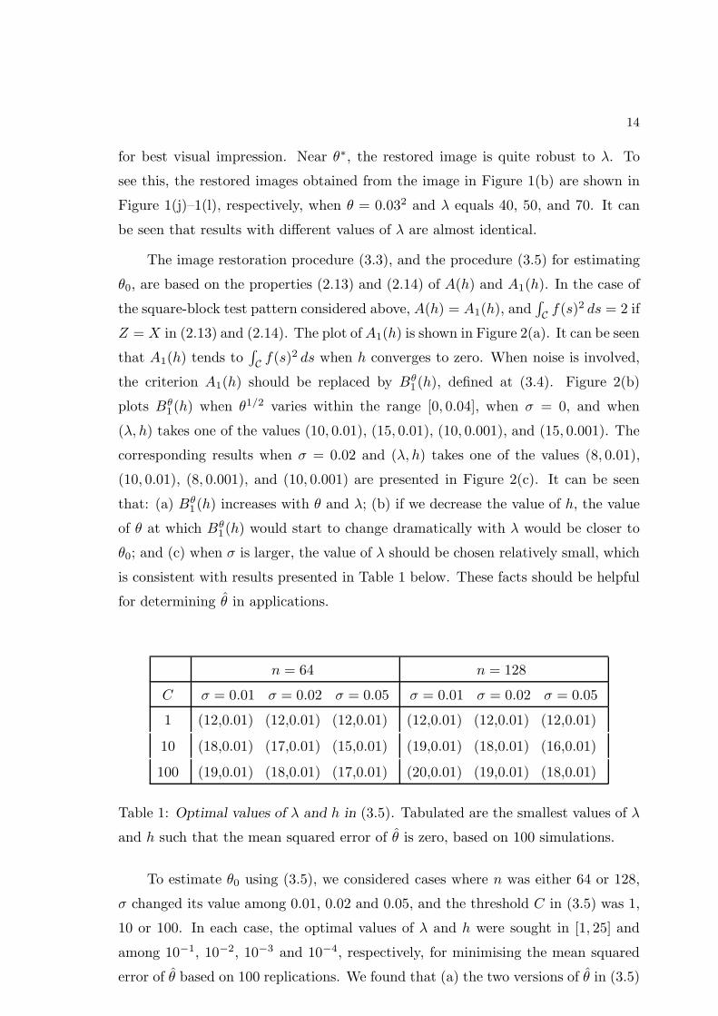
n = 64 n = 128

C σ = 0.01 σ = 0.02 σ = 0.05 σ = 0.01 σ = 0.02 σ = 0.05

1 (12,0.01) (12,0.01) (12,0.01) (12,0.01) (12,0.01) (12,0.01)

10 (18,0.01) (17,0.01) (15,0.01) (19,0.01) (18,0.01) (16,0.01)

100 (19,0.01) (18,0.01) (17,0.01) (20,0.01) (19,0.01) (18,0.01)

Table 1: Optimal values of λ and h in (3.5). Tabulated are the smallest values of λ

and h such that the mean squared error of θ is zero, based on 100 simulations.

To estimate θ0 using (3.5), we considered cases where n was either 64 or 128,

σ changed its value among 0.01, 0.02 and 0.05, and the threshold C in (3.5) was 1,

10 or 100. In each case, the optimal values of λ and h were sought in [1, 25] and

among 10−1, 10−2, 10−3 and 10−4, respectively, for minimising the mean squared

error of θ based on 100 replications. We found that (a) the two versions of θ in (3.5)

15

gave exactly the same results in all cases, and (b) in each case we could always find

values of λ and h such that mean squared error vanished (i.e., θ = θ0) in all 100

replications. The smallest values of λ and h for which mean squared error vanished

are listed in Table 1. It can be seen that the optimal value of h is stable when n, σ

and C change. The value of λ should be chosen larger when n is larger, when σ is

smaller, or when C is larger.

Image analysis enjoys an advantage that smoothing methods applied to related

problems do not: even if an observer has never seen the true image, he or she often

has an accurate impression, gained from extensive experience, of the scene to which

the degraded image is an approximation. It is appropriate, and very common in

practice, to exploit this information and choose tuning parameters so as to produce a

restoration that gives the best visual impression. This approach has the advantage

that it is not limited by metric-based, technical accounts of performance. While

commonly used in theoretical work, those approaches are well-known not to respect

perceived visual fidelity. See, for example, Marron and Tsybakov (1995).

4.2. Lena image example. Next we applied our image restoration procedure, de-

scribed by (3.3)–(3.5), to the Lena image. The original Lena image shown in Fig-

ure 3(a) has 256 × 256 pixels, with grey levels in the range [0, 255]. Its version

degraded by the Gaussian point-spread function (2.3), with θ0 = 0.0152, and by

independent and identically distributed noise from the N(0, 1) distribution, is illus-

trated in Figure 3(b).

The criterion Bθ1(h) is shown in Figure 3(c) when λ = 20 or 25, and h = 0.01

or 0.001. It can be seen from the plot that Bθ1(h) starts to increase dramatically

around θ = 0.0152 when λ increases from 20 to 25, and when h = 0.001. In (3.5),

if we chose C = 1000 then we obtained θ = 0.0152 when λ ≥ 20 and h = 0.001.

Combining these two facts, it can be concluded that θ0 is close to 0.0152. In

applications, we can also obtain a reasonable estimator of θ0 by trying several

values of θ. The restored Lena images, using the method at (3.3) when λ = 1000 and

θ = 0.012, 0.0142, 0.0152, 0.0162 or 0.022, are shown in Figure 3(d)–(h), respectively.

From these plots it can be seen that the restored images are quite good when θ is

close to θ0; compare Figure 3(e)–(g).

The restored image defined at (3.3) was obtained using an inverse filter with

hard thresholding. In the literature there are several other procedures for recovering

16

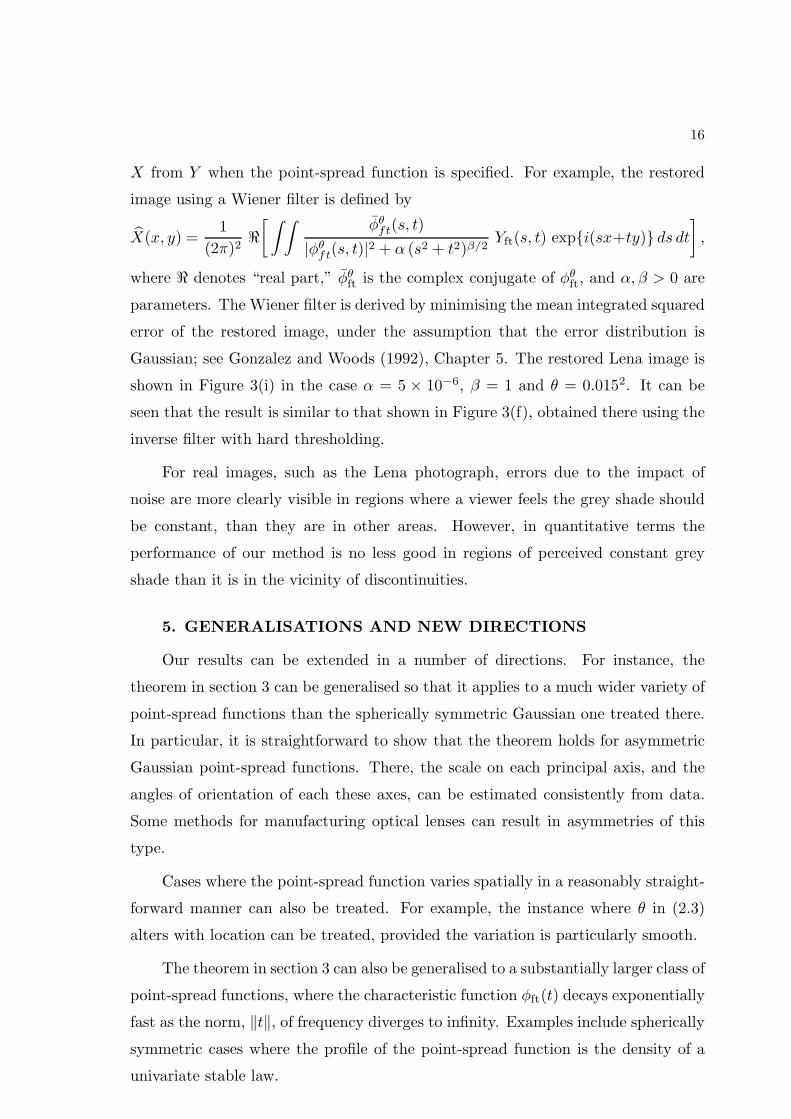
X from Y when the point-spread function is specified. For example, the restored

image using a Wiener filter is defined by

X(x, y) =1

(2π)2ℜ

[ ∫ ∫φθ

ft(s, t)

|φθft(s, t)|2 + α (s2 + t2)β/2

Yft(s, t) exp{i(sx+ty)} ds dt],

where ℜ denotes “real part,” φθft is the complex conjugate of φθ

ft, and α, β > 0 are

parameters. The Wiener filter is derived by minimising the mean integrated squared

error of the restored image, under the assumption that the error distribution is

Gaussian; see Gonzalez and Woods (1992), Chapter 5. The restored Lena image is

shown in Figure 3(i) in the case α = 5 × 10−6, β = 1 and θ = 0.0152. It can be

seen that the result is similar to that shown in Figure 3(f), obtained there using the

inverse filter with hard thresholding.

For real images, such as the Lena photograph, errors due to the impact of

noise are more clearly visible in regions where a viewer feels the grey shade should

be constant, than they are in other areas. However, in quantitative terms the

performance of our method is no less good in regions of perceived constant grey

shade than it is in the vicinity of discontinuities.

5. GENERALISATIONS AND NEW DIRECTIONS

Our results can be extended in a number of directions. For instance, the

theorem in section 3 can be generalised so that it applies to a much wider variety of

point-spread functions than the spherically symmetric Gaussian one treated there.

In particular, it is straightforward to show that the theorem holds for asymmetric

Gaussian point-spread functions. There, the scale on each principal axis, and the

angles of orientation of each these axes, can be estimated consistently from data.

Some methods for manufacturing optical lenses can result in asymmetries of this

type.

Cases where the point-spread function varies spatially in a reasonably straight-

forward manner can also be treated. For example, the instance where θ in (2.3)

alters with location can be treated, provided the variation is particularly smooth.

The theorem in section 3 can also be generalised to a substantially larger class of

point-spread functions, where the characteristic function φft(t) decays exponentially

fast as the norm, ‖t‖, of frequency diverges to infinity. Examples include spherically

symmetric cases where the profile of the point-spread function is the density of a

univariate stable law.

17

It is also possible to explore, in more detail, cases where our method does not

perform so well, for example those discussed in Section 2.6. Take, for example, the

case where the point-spread function is “rough but not too rough,” in the sense

that it is not infinitely differentiable but (unlike the circular-exponential example

discussed at (2.4)) has a number of bounded derivatives. The extent to which our

method works can be quantified theoretically by taking first the limit as δ converges

to zero, and then permitting the number of derivatives of the point-spread function

to increase. On the other hand, if the number of derivatives is not large then fitting

the wrong model (e.g. a Gaussian model, even if it is incorrect) may sometimes give

acceptable results.

More broadly, limitations of the models and methodology we have developed

can be explored. Note that the point-spread function model exemplified by (2.1)

and (3.1) is appropriate only in the setting of a linear filter. Non-linear filters cannot

be removed so readily; in general, our approach would find it difficult to distinguish

non-linear filters from noise. Conversely, our approach would confuse noise added

to the image, before blur, with the true image, and would fail to suppress noise in

such cases. Methods quite different from those that we have discussed are needed

to deal with problems such as this.

APPENDIX A.1: INTEGRALS OF SQUARED DIFFERENCES

OF IMAGES

Let C denote a curve in the plane, having a continuously turning tangent, except

possibly for a finite number of jump discontinuities in the tangent (giving corners

of C); assume C is of finite length and, for the present, is neither disconnected nor

self-intersecting; let f denote a continuous function from C to the real line; and, for

points in IR2 close to but not on C, identify two sides, S1 and S2 say, of C. Let X

be a compactly supported function from IR2 to IR, with the property that (a) both

partial derivatives of X are bounded uniformly in (x, y) ∈ IR2 \ C, and (b) if s ∈ Cthen X(s1) −X(s2) → f(s) as sj → s for j = 1, 2, with sj on side Sj of C. Define

A(h) as at (2.10), although for the function X instead of Z. Then (2.13) holds.

More generally, we do not need to confine attention to instances where the im-

age X includes a single, non-self intersecting curve along which a fault-type discon-

tinuity occurs. General cases may be constructed by taking X = X0 to be the sum

of any finite number of functions X1, . . . , Xm say, each of which has the properties

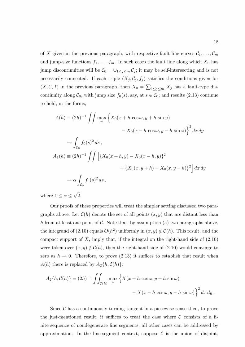
18

of X given in the previous paragraph, with respective fault-line curves C1, . . . , Cm

and jump-size functions f1, . . . , fm. In such cases the fault line along which X0 has

jump discontinuities will be C0 = ∪1≤j≤m Cj ; it may be self-intersecting and is not

necessarily connected. If each triple (Xj, Cj , fj) satisfies the conditions given for

(X, C, f) in the previous paragraph, then X0 =∑

1≤j≤m Xj has a fault-type dis-

continuity along C0, with jump size f0(s), say, at s ∈ C0; and results (2.13) continue

to hold, in the forms,

A(h) ≡ (2h)−1

∫ ∫max

ω

{X0(x+ h cosω, y + h sinω)

−X0(x− h cosω, y − h sinω)}2

dx dy

→∫

C0

f0(s)2 ds ,

A1(h) ≡ (2h)−1

∫ ∫ [{X0(x+ h, y) −X0(x− h, y)}2

+ {X0(x, y + h) −X0(x, y − h)}2]dx dy

→ α

∫

C0

f0(s)2 ds ,

where 1 ≤ α ≤√

2.

Our proofs of these properties will treat the simpler setting discussed two para-

graphs above. Let C(h) denote the set of all points (x, y) that are distant less than

h from at least one point of C. Note that, by assumption (a) two paragraphs above,

the integrand of (2.10) equals O(h2) uniformly in (x, y) /∈ C(h). This result, and the

compact support of X , imply that, if the integral on the right-hand side of (2.10)

were taken over (x, y) /∈ C(h), then the right-hand side of (2.10) would converge to

zero as h → 0. Therefore, to prove (2.13) it suffices to establish that result when

A(h) there is replaced by A2{h, C(h)}:

A2{h, C(h)} = (2h)−1

∫ ∫

C(h)

maxω

{X(x+ h cosω, y + h sinω)

−X(x− h cosω, y − h sinω)}2

dx dy .

Since C has a continuously turning tangent in a piecewise sense then, to prove

the just-mentioned result, it suffices to treat the case where C consists of a fi-

nite sequence of nondegenerate line segments; all other cases can be addressed by

approximation. In the line-segment context, suppose C is the union of disjoint,

19

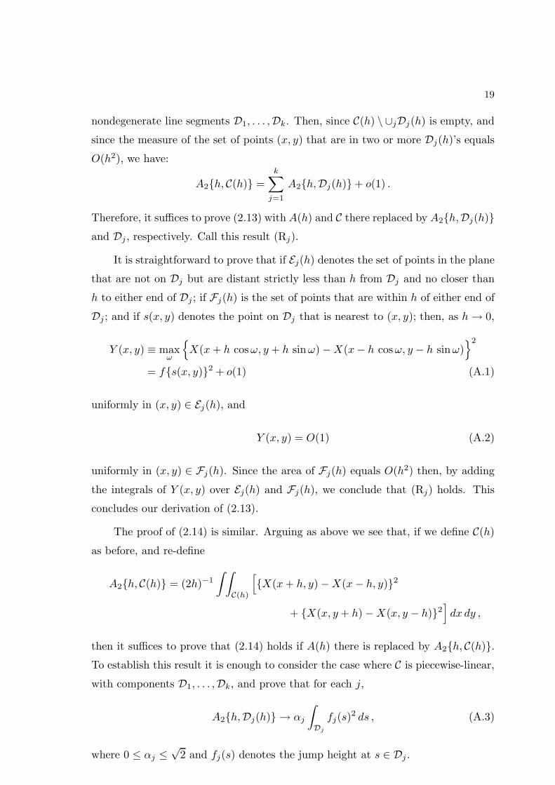
nondegenerate line segments D1, . . . ,Dk. Then, since C(h) \ ∪jDj(h) is empty, and

since the measure of the set of points (x, y) that are in two or more Dj(h)’s equals

O(h2), we have:

A2{h, C(h)} =k∑

j=1

A2{h,Dj(h)} + o(1) .

Therefore, it suffices to prove (2.13) with A(h) and C there replaced by A2{h,Dj(h)}and Dj , respectively. Call this result (Rj).

It is straightforward to prove that if Ej(h) denotes the set of points in the plane

that are not on Dj but are distant strictly less than h from Dj and no closer than

h to either end of Dj ; if Fj(h) is the set of points that are within h of either end of

Dj ; and if s(x, y) denotes the point on Dj that is nearest to (x, y); then, as h→ 0,

Y (x, y) ≡ maxω

{X(x+ h cosω, y + h sinω) −X(x− h cosω, y − h sinω)

}2

= f{s(x, y)}2 + o(1) (A.1)

uniformly in (x, y) ∈ Ej(h), and

Y (x, y) = O(1) (A.2)

uniformly in (x, y) ∈ Fj(h). Since the area of Fj(h) equals O(h2) then, by adding

the integrals of Y (x, y) over Ej(h) and Fj(h), we conclude that (Rj) holds. This

concludes our derivation of (2.13).

The proof of (2.14) is similar. Arguing as above we see that, if we define C(h)

as before, and re-define

A2{h, C(h)} = (2h)−1

∫ ∫

C(h)

[{X(x+ h, y) −X(x− h, y)}2

+ {X(x, y+ h) −X(x, y − h)}2]dx dy ,

then it suffices to prove that (2.14) holds if A(h) there is replaced by A2{h, C(h)}.To establish this result it is enough to consider the case where C is piecewise-linear,

with components D1, . . . ,Dk, and prove that for each j,

A2{h,Dj(h)} → αj

∫

Dj

fj(s)2 ds , (A.3)

where 0 ≤ αj ≤√

2 and fj(s) denotes the jump height at s ∈ Dj .

20

Let Ej(h) and Fj(h) be as in the proof of (2.13), and introduce GVj (h) and

GHj (h) as the sets of points in Ej(h) that are distant strictly less than h from Dj

in the vertical and horizontal directions, respectively, and HVj (h) and HH

j (h) as the

sets of points in Ej(h) that are strictly further than h from Dj in the vertical and

horizontal directions, respectively. Recall that s(x, y) denotes the point on Dj that

is nearest to (x, y). Then, in place of (A.1),

{X(x+ h, y) −X(x− h, y)}2 = f{s(x, y)}2 + o(1) , uniformly in (x, y) ∈ GHj (h) ,

{X(x, y+ h) −X(x, y − h)}2 = f{s(x, y)}2 + o(1) , uniformly in (x, y) ∈ GVj (h) ,

and in place of (A.2),

{X(x+ h, y) −X(x− h, y)}2 + {X(x, y + h) −X(x, y − h)}2 = O(1)

uniformly in (x, y) ∈ Fj(h). Additionally,

{X(x+ h, y) −X(x− h, y)}2 = O(h2

), uniformly in (x, y) ∈ HH

j (h) ,

{X(x, y + h) −X(x, y − h)}2 = O(h2

), uniformly in (x, y) ∈ HV

j (h) .

Combining these results, and defining DHj [respectively, DV

j ] to be the set of x

(respectively, y) such that (x, y) ∈ Dj for some y (for some x), we deduce that

(2h)−1

∫ ∫

Dj(h)

{X(x+ h, y) −X(x− h, y)}2 dx dy

= (2h)−1

∫ ∫

GH

j(h)

{X(x+ h, y) −X(x− h, y)}2 dx dy + o(1)

=

∫

DH

j

f{s(x, y)}2 dx+ o(1) , (A.4)

(2h)−1

∫ ∫

Dj(h)

{X(x, y + h) −X(x, y− h)}2 dx dy

=

∫

DV

j

f{s(x, y)}2 dy + o(1) . (A.5)

Assume Dj(h) is inclined at angle ω ∈ [0, π/2] to the positive direction of the

horizontal axis. (Other orientations may be treated similarly.) Combining (A.4)

and (A.5) we deduce that

A2{h,Dj(h)} →∫

DH

j

f{s(x, y)}2 dx+

∫

DV

j

f{s(x, y)}2 dy

= (cosω + sinω)

∫

Dj

f{s(x, y)}2 ds . (A.6)

21

Since 1 ≤ cosω + sinω ≤√

2 then (A.3) follows from (A.6).

APPENDIX A.2: PROOFS FOR SQUARE-BLOCK TEST-PATTERN

Using Parseval’s identity it may be proved that if the function Z has Fourier

transform Zft, and if A1(h) is given by (2.11), then

A1(h) = 2h−1 (2π)2∫ ∫

|Zft(s, t)|2(sin2 sh+ sin2 th

)ds dt . (A.7)

If we take Z = X , where X denotes the function defining the square-block test-

pattern, then the fact that the sides of the pattern are parallel to the coordinate

axes, and of equal length and height, implies that A1 = A, and so A(h) is also given

by (A.7).

The Fourier transform of the square-block test-pattern function X , given at

(2.6), is

Xft(s, t) =sin s sin t

π2 st,

and the Fourier transform of Zθ, given by (2.7), is

Zθft = φθ0

ft Xft

/φθ

ft . (A.8)

Hence, by (A.7), the version of A1(h) for Zθ is

A1(h) =16

hπ2

∫ ∫ (sin s sin t

st

)2 {φθ0

ft (s, t)

φθ(s, t)

}2

(sin sh)2 ds dt . (A.9)

We stated in Section 2.5 that if the function X contains fault-type discontinu-

ities, if φθ satisfies (2.9), and if θ > θ0, then A(h) = A1(h) = ∞ for each h > 0. We

prove this result here for the square-block test-pattern, showing that if θ > θ0 then

A1(h) = ∞. The infiniteness of A(h) then follows via (2.12). Now, (2.9) implies

that if θ > θ0 then for each C > 0,

A1(h) > const.

∫ ∫ (sin s sin t

st

)2

(1 + |s| + |t|)C (sin sh)2 ds dt ,

which is clearly infinite if C ≥ 2.

Next we prove that if φθ = φθexp denotes the circular-exponential point-spread

function at (2.4), if θ0 is positive but otherwise arbitrary, and if we apply the

difference operators A(h) and A1(h) to Z = Zθ given at (2.7), then (a) for each

θ > 0, Zθ is square-integrable, and (b) A1(h) → C1 (θ/θ0)6 as h→ 0, where C1 > 0

22

does not depend on θ or θ0. We know from (2.12) that A1(h) is a lower bound

to 2A(h), and in fact a longer argument will show that A(h) → C2 (θ/θ0)6, where

C2 > 0.

It can be proved that for each θ > 0,

φθft(s, t) is real-valued, strictly positive for all (s, t), and satisfies φθ

ft(s, t) ∼C3 θ

−3 (s2 + t2)−3/2 as |s| + |t| → ∞, where C3 > 0 denotes a constant.(A.10)

This property and (A.8) imply that Zθft, and hence (by Parseval’s identity) Zθ itself,

are square-integrable, thus giving (a) above.

Define J =∫(t−1 sin t)2 dt, where, here and below, integrals are taken over the

whole real line. Combining (A.9) and (A.10) we deduce that, for a constant C4 > 0

not depending on θ or θ0,

A1(h) ∼C4 θ

6

h θ06

∫ ∫ (sin s sin t

st

)2

(sin sh)2 ds dt

=C4 J θ

6

θ06

∫ (sin s

s

)2

sin2(s/h) ds→ C4 J2 θ6

2 θ06 .

That is, A1(h) → C (θ/θ0)6 as h→ 0, where C > 0, and so (b) above is true.

APPENDIX A.3: PROOF OF THEOREM

Let φθft denote the Fourier transform defined at (2.8), and let Xft be the con-

ventional Fourier transform of X :

Xft(s, t) =1

(2π)2

∫ ∫X(x, y) exp{−(isx+ ity)} dx dy .

The Fourier transform of φθ0X equals the product φθ0

ft Xft and differs from

(φθ0X

)tft

(s, t) =1

(2π)2

∫ ∫

Rr

(φθ0X

)(x, y) exp{−(isx+ ity)} dx dy

only in terms of order exp(−c1r2), i.e., for a constant c1 > 0:

sup(s,t)∈IR2

∣∣(φθ0X)tft − φθ0

ft (s, t)Xft(s, t)∣∣ = O

{exp

(− c1r

2)}. (A.11)

Taking the truncated Fourier transform of both sides of (3.1), we deduce that

Y θ0

tft =(φθ0X

)tft

+ δ wtft , (A.12)

23

where

wtft(s, t) =1

(2π)2

∫ ∫

Rr

exp{−(isx+ ity)} dW (x, y) . (A.13)

Put g1(s, t) = φθ0

ft (s, t)Xft(s, t)/φθft(s, t) and

g2(s, t) = δwtft(s, t)

φθft(s, t)

+O[exp

{12 θ

(s2 + t2

)− c1r

2}], (A.14)

where the big-oh term is interpreted as purely deterministic. Then, combining

(A.11) and (A.12), we may write:

Y θ0

tft (s, t)

φθft(s, t)

= g1(s, t) + g2(s, t) , (A.15)

uniformly in (s, t) ∈ IR2.

For j = 1, 2 define

Dj = Dθj (h) = 2h−1 (2π)2

∫ ∫|gj(s, t)|2

(sin2 sh+ sin2 th

)I(s2 + t2 ≤ λ2

)ds dt .

(A.16)

In view of (3.4) and (A.15),

∣∣Bθ1 −Dθ

1

∣∣ ≤ Dθ2 + 2

(Dθ

1 Dθ2

)1/2. (A.17)

By treating separately the real and imaginary parts of wtft, it may be proved from

(A.13) that for a constant C > 0, and with probability 1,

sups2+t2≤λ2

|wtft(s, t)| = O{(r | log δ|)C

}.

Using this bound, and the fact that

supu

[{min

(1, u2

)}−1sin2 u

]<∞ , (A.18)

we may deduce from (A.14) and (A.16) that for each c2 > 0 and some C > 0, and

with probability 1,

Dθ2(h) = O

[δ rC exp

{(θ + c2)λ

2}

+ exp{(θ + c2)λ

2 − 2c1r2}]

→ 0 , (A.19)

uniformly in 0 < θ < θ1 for any θ1 > 0, where the limit result follows from (3.8).

Furthermore,

Dθ1(h) = 2h−1 (2π)2

∫ ∫|Xft(s, t)|2 exp

{(θ − θ0)

(s2 + t2

)}

×(sin2 sh+ sin2 th

)I(s2 + t2 ≤ λ2

)ds dt .

24

This quantity is clearly a monotone increasing function of θ. Since X is bounded

and compactly supported then Xft is bounded, and so by (A.18),

h−1Dθ1(h) is bounded uniformly in h, λ > 0 and in 0 ≤ θ ≤ θ1, for any

θ1 ∈ [0, θ0).(A.20)

Suppose, on the other hand, that θ2 > θ0 and 0 < c1 < c2 <∞. Then, noting that

hλ→ ∞, we see that if δ is sufficiently small we have for all θ ≥ θ2,

Dθ1(h) ≥ 2h−1 (2π)2

∫ ∫|Xft(s, t)|2 exp

{(θ2 − θ0)

(s2 + t2

)}

×(sin2 sh+ sin2 th

)I{c1 ≤

(s2 + t2

)h2 ≤ c2

}ds dt .

Choose c1, c2 so that the interval [c1, c2] does not contain an integer multiple of π2.

Then there exists C1 > 0 such that, for all sufficiently small δ, sin2(sh)+sin2(th) ≥C1 for all (s, t) that satisfy c1 ≤ (s2 + t2) h2 ≤ c2. Therefore, with C2 = 8π2C1 we

have:

Dθ1(h) ≥ C2 h

−1 exp{(θ2 − θ0) h

−2 c1}

×∫ ∫

|Xft(s, t)|2 I{c1 ≤

(s2 + t2

)h2 ≤ c2

}ds dt .

This bound and (3.6) imply that for constants C3 > 0 and C4,

Dθ1(h) ≥ C3 h

C4 exp{(θ2 − θ0) h

−2 c1}

uniformly in θ ≥ θ2 . (A.21)

The theorem follows from (A.17) and (A.19)–(A.21).

REFERENCES

Brwon, L.D., Cai, T.T., Low, M.G., and Zhang, C.H. (2002). Asymptotic equiva-lence theory for nonparametric regression with random design. Ann. Statist.

30, 688–707.

Brown, L.D., and Low, M.G. (1996). Asymptotic equivalence of nonparametric re-

gression and white noise. Ann. Statist. 24, 2384–2398.

Carasso, A.S. (2001). Direct blind deconvolution. SIAM J. Appl. Math. 61, 1980–

2007.

Carasso, A.S. (2004). Singular integrals, image smoothness, and the recovery of

texture in image deblurring. SIAM J. Appl. Math. 64, 1749–1774.

Cornford, D., Csato, L., Evans, D.J., and Opper, M. (2004). Bayesian analysis of

the scatterometer wind retrieval inverse problem: some new approaches. J.

R. Statist. Soc. Ser. B 66, 609–626.

Doucet, A., Godsill, S.J., and Robert, C.P. (2002). Marginal maximum a posteriori

estimation using Markov chain Monte Carlo. Statist. Comput. 12, 77–84.

25

Ellis, S.P. (2002). Blind deconvolution when noise is symmetric: existence and ex-amples of solutions. Ann. Inst. Statist. Math. 54, 758–767.

Erdogmus, D., Hild, K.E., Principe, J.C., Lazaro, M., and Santamaria, I. (2004).Adaptive blind deconvolution of linear channels using Renyi’s entropy with

Parzen window estimation. IEEE Trans. Signal Process. 52, 1489–1498.

Figueiredo, M.A.T., and Nowak, R.D. (2003). An EM algorithm for wavelet-based

image restoration. IEEE Trans. Image Process. 12, 906–916.

Galatsanos, N.P., Mesarovic, V.Z., Molina, R., Katsaggelos, A.K., and Mateos, J.(2002). Hyperparameter estimation in image restoration problems with par-

tially known blurs. Opt. Eng. 41, 1845–1854.

Gassiat, E., and Gautherat, E. (1999). Speed of convergence for the blind decon-

volution of a linear system with discrete random input. Ann. Statist. 27,1684–1705.

Gonzalez, R.C., and Woods, R.E. (1992). Digital Image Processing. Addison-Wesley,New York.

Haario, H., Laine, M., Lehtinen, M., Saksman, E., and Tamminen, J. (2004). Markovchain Monte Carlo methods for high dimensional inversion in remote sens-

ing. J. R. Statist. Soc. Ser. B 66, 591–607.

Higdon, D., and Yamamoto, S. (2001). Estimation of the head sensitivity function in

scanning magnetoresistance microscopy. J. Amer. Statist. Assoc. 96, 785–793.

Johnstone, I.M., Kerkyacharian, G., Picard, D., and Raimondo, M. (2004). Waveletdeconvolution in a periodic setting. J. R. Statist. Soc. Ser. B 66, 547–573.

Kundur, D., and Hatzinakos, D. (1998). A novel blind deconvolution scheme forimage restoration using recursive filtering. IEEE Trans. Sig. Process. 46,

375–389.

Li, K.C., and Shedden, K. (2001). Monte Carlo deconvolution of digital signals

guided by the inverse filter. J. Amer. Statist. Assoc. 96, 1014–1021.

Likas A.C., and Galatsanos, N.P. (2004). A variational approach for Bayesian blindimage deconvolution. IEEE Trans. Signal Process. 52, 2222–2233.

Marron, J.S., and Tsybakov, A.B. (1995). Visual error criteria for qualitative smooth-ing. J. Amer. Statist. Assoc. 90, 499–507.

May, K.L., Stathaki, T., and Katsaggelos, A.K. (2003). Spatially adaptive intensitybounds for image restoration. EURASIP J. Appl. Sig. Process. 2003, 1167–

1180.

Nussbaum, M. (1996). Asymptotic equivalence of density estimation and Gaussian

white noise. Ann. Statist. 24, 2399–2430.

Poskitt, D.S., Dougancay, K., and Chung, S.H. (1999). Double-blind deconvolution:

the analysis of post-synaptic currents in nerve cells. J. R. Statist. Soc. Ser. B61, 191–212.

Rosec, O., Boucher, J.M., Nsiri, B., and Chonavel, T. (2003). Blind marine seismic

26

deconvolution using statistical MCMC methods. IEEE J. Oceanic Eng. 28,502–512.

Sotthivirat, S., and Fessler, J.A. (2003). Relaxed ordered-subset algorithm for penalized-likelihood image restoration. J. Opt. Soc. Amer. Ser. A 20, 439–449.

Wolfe, P.J., Godsill, S.J., and Ng, W.-J. (2004). Bayesian variable selection and reg-

ularization for time-frequency surface estimation. J. R. Statist. Soc. Ser. B

66, 575–589.

Zhang L.Q., Amari, S., and Cichocki, A. (2001). Semiparametric model and super-efficiency in blind deconvolution. Sig. Process. 81, 2535–2553.