Blind Adaptive Compensation of I/Q Mismatch and Frequency Offset in Low-IF Receivers
6
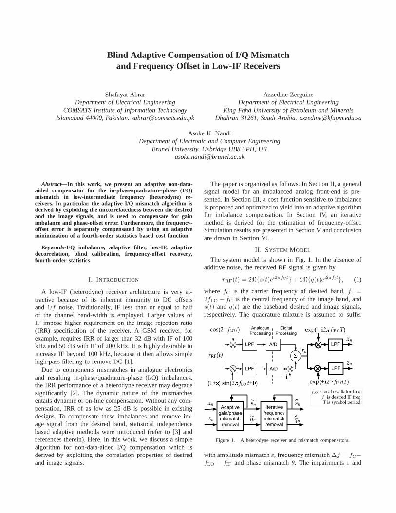
Blind Adaptive Compensation of I/Q Mismatch and Frequency Offset in Low-IF Receivers Shafayat Abrar Department of Electrical Engineering COMSATS Institute of Information Technology Islamabad 44000, Pakistan. [email protected] Azzedine Zerguine Department of Electrical Engineering King Fahd University of Petroleum and Minerals Dhahran 31261, Saudi Arabia. [email protected] Asoke K. Nandi Department of Electronic and Computer Engineering Brunel University, Uxbridge UB8 3PH, UK [email protected] Abstract—In this work, we present an adaptive non-data- aided compensator for the in-phase/quadrature-phase (I/Q) mismatch in low-intermediate frequency (heterodyne) re- ceivers. In particular, the adaptive I/Q mismatch algorithm is derived by exploiting the uncorrelatedness between the desired and the image signals, and is used to compensate for gain imbalance and phase-offset error. Furthermore, the frequency- offset error is separately compensated by using an adaptive minimization of a fourth-order statistics based cost function. Keywords-I/Q imbalance, adaptive filter, low-IF, adaptive decorrelation, blind calibration, frequency-offset recovery, fourth-order statistics I. I NTRODUCTION A low-IF (heterodyne) receiver architecture is very at- tractive because of its inherent immunity to DC offsets and 1/f noise. Traditionally, IF less than or equal to half of the channel band-width is employed. Larger values of IF impose higher requirement on the image rejection ratio (IRR) specification of the receiver. A GSM receiver, for example, requires IRR of larger than 32 dB with IF of 100 kHz and 50 dB with IF of 200 kHz. It is highly desirable to increase IF beyond 100 kHz, because it then allows simple high-pass filtering to remove DC [1]. Due to components mismatches in analogue electronics and resulting in-phase/quadrature-phase (I/Q) imbalances, the IRR performance of a heterodyne receiver may degrade significantly [2]. The dynamic nature of the mismatches entails dynamic or on-line compensation. Without any com- pensation, IRR of as low as 25 dB is possible in existing designs. To compensate these imbalances and remove im- age signal from the desired band, statistical independence based adaptive methods were introduced (refer to [3] and references therein). Here, in this work, we discuss a simple algorithm for non-data-aided I/Q compensation which is derived by exploiting the correlation properties of desired and image signals. The paper is organized as follows. In Section II, a general signal model for an imbalanced analog front-end is pre- sented. In Section III, a cost function sensitive to imbalance is proposed and optimized to yield into an adaptive algorithm for imbalance compensation. In Section IV, an iterative method is derived for the estimation of frequency-offset. Simulation results are presented in Section V and conclusion are drawn in Section VI. II. SYSTEM MODEL The system model is shown in Fig. 1. In the absence of additive noise, the received RF signal is given by r RF (t)=2ℜ{s(t)e i2πfCt } +2ℜ{q(t)e i2πfIt }, (1) where f C is the carrier frequency of desired band, f I = 2f LO − f C is the central frequency of the image band, and s(t) and q(t) are the baseband desired and image signals, respectively. The quadrature mixture is assumed to suffer LPF A/D LPF A/D rRF(t) cos(2 fLO t) (1+ ) sin(2 fLO t+ ) i LPF LPF exp( i2 fIF nT) exp(+i2 fIF nT) r n xn z n Analogue Processing Digital Processing fLO is local oscillator freq. fIF is desired IF freq. T is symbol period. xn z n Adaptive gain/phase mismatch removal s n qn Iterative frequency mismatch removal s n q n ~ ~ ˆ ˆ Figure 1. A heterodyne receiver and mismatch compensators. with amplitude mismatch ε, frequency mismatch Δf = f C − f LO − f IF and phase mismatch θ. The impairments ε and
-
Upload
shafayat-abrar -
Category
Documents
-
view
220 -
download
1
description
In this work, we present an adaptive non-dataaided compensator for the in-phase/quadrature-phase (I/Q)mismatch in low-intermediate frequency (heterodyne) receivers.In particular, the adaptive I/Q mismatch algorithm is derived by exploiting the uncorrelatedness between the desired and the image signals, and is used to compensate for gain imbalance and phase-offset error. Furthermore, the frequencyoffset error is separately compensated by using an adaptive minimization of a fourth-order statistics based cost function.
Transcript of Blind Adaptive Compensation of I/Q Mismatch and Frequency Offset in Low-IF Receivers
Blind Adaptive Compensation of I/Q Mismatchand Frequency Offset in Low-IF Receivers
Shafayat AbrarDepartment of Electrical Engineering
COMSATS Institute of Information TechnologyIslamabad 44000, Pakistan. [email protected]
Azzedine ZerguineDepartment of Electrical Engineering
King Fahd University of Petroleum and MineralsDhahran 31261, Saudi Arabia. [email protected]
Asoke K. NandiDepartment of Electronic and Computer Engineering
Brunel University, Uxbridge UB8 3PH, [email protected]
Abstract—In this work, we present an adaptive non-data-aided compensator for the in-phase/quadrature-phase (I/Q)mismatch in low-intermediate frequency (heterodyne) re-ceivers. In particular, the adaptive I/Q mismatch algorithm isderived by exploiting the uncorrelatedness between the desiredand the image signals, and is used to compensate for gainimbalance and phase-offset error. Furthermore, the frequency-offset error is separately compensated by using an adaptiveminimization of a fourth-order statistics based cost function.
Keywords-I/Q imbalance, adaptive filter, low-IF, adaptivedecorrelation, blind calibration, frequency-offset recovery,fourth-order statistics
I. I NTRODUCTION
A low-IF (heterodyne) receiver architecture is very at-tractive because of its inherent immunity to DC offsetsand 1/f noise. Traditionally, IF less than or equal to halfof the channel band-width is employed. Larger values ofIF impose higher requirement on the image rejection ratio(IRR) specification of the receiver. A GSM receiver, forexample, requires IRR of larger than 32 dB with IF of 100kHz and 50 dB with IF of 200 kHz. It is highly desirable toincrease IF beyond 100 kHz, because it then allows simplehigh-pass filtering to remove DC [1].
Due to components mismatches in analogue electronicsand resulting in-phase/quadrature-phase (I/Q) imbalances,the IRR performance of a heterodyne receiver may degradesignificantly [2]. The dynamic nature of the mismatchesentails dynamic or on-line compensation. Without any com-pensation, IRR of as low as 25 dB is possible in existingdesigns. To compensate these imbalances and remove im-age signal from the desired band, statistical independencebased adaptive methods were introduced (refer to [3] andreferences therein). Here, in this work, we discuss a simplealgorithm for non-data-aided I/Q compensation which isderived by exploiting the correlation properties of desiredand image signals.
The paper is organized as follows. In Section II, a generalsignal model for an imbalanced analog front-end is pre-sented. In Section III, a cost function sensitive to imbalanceis proposed and optimized to yield into an adaptive algorithmfor imbalance compensation. In Section IV, an iterativemethod is derived for the estimation of frequency-offset.Simulation results are presented in Section V and conclusionare drawn in Section VI.
II. SYSTEM MODEL
The system model is shown in Fig. 1. In the absence ofadditive noise, the received RF signal is given by
rRF(t) = 2ℜs(t)ei2πfCt+ 2ℜq(t)ei2πfIt, (1)
where fC is the carrier frequency of desired band,fI =2fLO − fC is the central frequency of the image band, ands(t) and q(t) are the baseband desired and image signals,respectively. The quadrature mixture is assumed to suffer
LPF A/D
LPF A/D
rRF(t)
cos(2 fLO t)
(1+ ) sin(2 fLO t+ )i
LPF
LPF
exp( i2 fIFnT)
exp(+i2 fIFnT)
rn
xn
zn
Analogue
Processing
Digital
Processing
fLO is local oscillator freq.fIF is desired IF freq. T is symbol period.xn
zn
Adaptive
gain/phase
mismatch
removal
sn
qn
Iterative
frequency
mismatch
removal
sn
qn~
~ ˆ
ˆ
Figure 1. A heterodyne receiver and mismatch compensators.
with amplitude mismatchε, frequency mismatch∆f = fC−fLO − fIF and phase mismatchθ. The impairmentsε and
θ are assumed to be frequency independent. The digital IFsignalrn, sampled at the rate of1/T , is expressed as:
rn = (βsn + αq∗n) e+i2πn(fIFT+Ω)
+ (βqn + αs∗n) e−i2πn(fIFT+Ω),
(2)
whereα = 0.5(1− (1 + ε)eiθ
), β = 0.5
(1 + (1 + ε)e−iθ
),
Ω = T∆f , sn = s(t)|t=nT and qn = q(t)|t=nT . Afterdown-conversion and low-pass filtering, we obtain the base-band signalsxn andzn:
xn = (βsn + αq∗n) e+i2πnΩ, (3a)
zn = (βqn + αs∗n) e−i2πnΩ. (3b)
The digital processor at receiver uses the baseband signalsxn and zn to estimate the impairments,θ, ǫ and Ω.Assuming that impairments are perfectly known, then thedesired and image signals are expressed as
sn = sne−i2πnΩ =
(1+γ∗
1−|γ|2
)(xn − γ z∗n) e
−i2πnΩ, (4a)
qn = qne+i2πnΩ =
(1+γ∗
1−|γ|2
)(zn − γ x∗
n) e+i2πnΩ, (4b)
whereγ = α/β∗. The impairmentsε andθ are related toγ,we can show:
θ = angle
1− γ
1 + γ
, and ε =
∣∣∣∣1− γ
1 + γ
∣∣∣∣− 1. (5)
III. E XISTING SOLUTIONS FORM ISMATCH
COMPENSATION
A method is presented in [5] for correcting the gain andphase imbalances and the bias errors of the in-phase andquadrature channels of a coherent signal processor by meansof coefficients which are derived from measurements of atest signal. The residual errors after correction depend uponthe signal-to-noise ratio (S/N) of the test signal and the de-gree of filtering used in deriving the correction coefficients.According to [6] “this correction can be applied only onefrequency at a time. When theI andQ channels cover awide bandwidth, the imbalance is a function of frequency.This method might be impractical to apply because it needsan off-line test input and can not track time variation”.
A solution mentioned in [7] is to move the generation ofI andQ signals to the digital domain by using the Hilberttransform. In this approach, the data for one channel (say theI channel) are obtained from a single-path A/D converter,while the data of theQ channel are generated by processingthe channel data through a Hilbert filter. According to [6],however, “the operating speed is limited by the complexityof Hilbert filters. In order to get balancedI andQ signals, ahigh-order filter is needed to perform the Hilbert transform.The resulting solution has high power consumption, lowprocessing speed, and high hardware complexity”.
In [6], authors proposed a two-tap (wx,n and wz,n)butterfly-structure adaptive filter which worked on the princi-ple of noise cancellation (de-correlation) and it was realized
as follows:
wx,n = wx,n−1 + µ sn q∗n (6a)
wz,n = wz,n−1 + µ qn s∗n (6b)
where sn and qn were obtained assn = xn − znwz,n−1
and qn = zn − xnwx,n−1. The above algorithm was simplebut heuristic in nature. Though it was explained to be ade-correlation process but it was not explained what costfunction was exactly being minimized or maximized. It alsooverlooked the fact thatwx,n = w∗
z,n which could have beenutilized to implement a simpler update.
In the year 2007, authors in [8] proposed a gradient-basedadaptive algorithm to compensate for I/Q imbalance in low-IF receivers. Here the compensation algorithm developmentsbuild on the so-called circular nature of complex-valuedcommunications waveforms which is known to hold onlyunder perfect I/Q balance. A well-behaving non-circularitymeasure is first formed which is then minimized iterativelyusing gradient-descent type approach. The derived compen-sator is computationally simple and operates blindly on thereceived signal, meaning that no known training or pilotdata is needed. In particular, they suggested to minimize thefollowing non-circularity measure:
γ† = argminγ
∣∣Eu2n
∣∣2, where un := xn − γx∗n. (7)
The true gradient of thisself-cancellationcost (7) wasmentioned to bebiased. Ignoring biased terms, however, anapproximate unbiased algorithm was obtained as follows:
γn ≈ γn−1 + µ(rncn − 2r2nγn−1 − γ∗
n−1c2n
)(8)
wherecn := λ ccn−1 + (1 − λ c)x2n andrn := λ rrn−1 +
(1− λ r) |xn|2. Detailed discussion on (7) appeared in [9].
Note that a simplified form of the update (8) appeared earlierin [1] (and later in [15]) but without the notion of circularity;they proposed two real-valued updates: (belowℜ and ℑdenote the real and imaginary parts, respectively)
ℜ[γn] = ℜ[γn−1] + µ(ℜ[un]
2 −ℑ[un]2),
ℑ[γn] = ℑ[γn−1] + 2µℜ[un]ℑ[un],(9)
whereun is as specified in (7). Note that (9) is equivalentto the following single-step complex-valued update:
γn = γn−1 + µu2n. (10)
The rational behind (9) is to design an update which ensuresEℜ[un]
2 = Eℑ[un]2 and Eℜ[un]ℑ[un] = 0 in steady-state
(which is nothing but circularity) and thus successfullyremoving the gain/phase related imbalances. The update(9) was proposed onheuristic ground and algorithmic de-velopment arising from some cost was not discussed. Animproved version of (10) is obtained in [10] by exploitingthe normalized least mean square filtering, as given by
γn = γn−1 + µu2n
|un|2. (11)

where the normalization factor serves to provide aγ-dependent factor. There are number of other adaptive com-pensators which are suitable for higher baud-rate block datatransfer; interested readers may refer to [11]-[22].
IV. ESTIMATION OF GAIN IMBALANCE γ
Exploiting the fact that the desired and image signalssnand qn are mutually uncorrelated, optimum closed-formestimates were obtained in [4] as follows:
γ(1)opt =
B −√B2 − 4|A|2
2A∗, (12a)
γ(2)opt =
B +√B2 − 4|A|2
2A∗, (12b)
where A := Exnzn, and B := E(|xn|
2 + |zn|2). For
vanishing imbalance, i.e.,A → 0, we haveγ(1)opt → 0 and
γ(2)opt → ∞. Note that authors in [4] preferred to use the root
with smaller magnitude, i.e.,γ(1)opt.
In this work, we propose to obtain the value ofγadaptively by minimizing a cost which is measure of thecorrelation between the estimated signals,sn and qn, math-ematically it is expressed as
γ† = argminγ
∣∣∣∣E (xn − γz∗n) (zn − γx∗n)
∣∣∣∣2
, (13)
Note that this cost is insensitive to frequency offset error,Ω, which facilitates separate estimation ofΩ. To obtain agradient-based adaptive algorithm forγ, we use
γn = γn−1 − µ(∇γ |C|2
)∗, (14)
for γ = γn−1 and C := E(xn − γn−1z∗n)(γn−1x
∗n − zn).
Note that the auxiliary variableC can be expressed asC =A−B γn−1 +A∗ γ2
n−1, whereA andB are as specified in(12); next, we find
∂|C|2
∂γn−1=
∂|C|2
∂C
∂C
∂γn−1= C∗ (2A∗ γn−1 −B) , (15)
Replacing the statisticsA, B and C with their respectiveestimates, we get the following gradient-based algorithm:
An = λ gAn−1 + (1− λ g)xnzn,
Bn = λ gBn−1 + (1− λ g)(|xn|
2 + |zn|2),
Cn = An −Bn γn−1 +A∗n γ
2n−1,
γn = γn−1 + µ g Cn
(Bn − 2An γ
∗n−1
),
(16)
where µ g is a positive step-size and0 < λ g < 1 isa forgetting-factor. SubstitutingAn and Bn in (12), weobtain γ
(1)n−1 and γ
(2)n−1 as the estimates ofγ(1)
opt and γ(2)opt,
respectively. Usingγ(1)n−1 andγ(2)
n−1, we can express (16) asfollows:
γn = γn−1 − η(γn−1 − γ
(1)n−1
)(γn−1 − γ
(2)n−1
)
×
(γn−1 −
γ(1)n−1 + γ
(2)n−1
2
)∗
,(17)
whereη = 2µ|A|2 and 0.5(γ(1)n−1 + γ
(2)n−1) is the estimate
of saddle point (see Fig. 2(a)). This implies that, dependingon initialization, the update may converge either toγ
(1)opt and
γ(2)opt. Under no imbalance condition, however, as one of the
roots is required to be zero, the update has a natural tendencyto converge to the root with smaller magnitude provided thatthe step-size is large enough to help escape the other root(see Fig. 2(b)-(c)). Also note that, unlike [8], the proposedalgorithm (16) is unbiased.
V. ESTIMATION OF FREQUENCYOFFSETΩ
A. For PSK Signals:
The presence of frequency-offset error contaminates theestimated signalsn by the factore+i2πnΩ. SupposeΩn−1 isthe available estimate ofΩ, then sn is expressed as
sn = sne−i2πnΩn−1
=1 + γ∗
n−1
1− |γn−1|2(xn − γn−1 z
∗n) e
−i2πnΩn−1 ,(18)
If sn is anm-PSK, then the maximum likelihood approachestimatesΩ, as given by,
Ω =angle
∑N
k=0
(sn−k s
∗n−1−k
)m
2πm, (19)
where N denotes number of symbols. Note that this es-timator assumes that the signal has constant modulus; inthe presence of gain imbalance, however, we would needgain normalization to ensure this property. Denoting∆n :=Ωn−1 − Ω, and assuming no additive noise, note that
(s ∗n−1sn
|sn−1| · |sn|
)m
=
(s ∗n−1e
i2π(n−1)Ωn−2 · sne−i2πnΩn−1
|sn−1| · |sn|
)m
≈(s∗n−1e
−i2π(n−1)∆n−1 · snei2πn∆n
)m
= ei2πm(∆n−1+n(∆n−∆n−1)),
(20)
Further assuming∆n ≈ ∆n−1, we obtain
∆n ≈1
2πmangle
(s ∗n−1sn
|sn−1| · |sn|
)m, (21)
With the aid of (21), an iterative estimate ofΩn is obtainedas
∆n = λ d∆n−1 + (1− λ d)
(s ∗n−1sn
|sn−1sn|
)m,
Ωn = λ oΩn−1 + (1− λ o)angle
∆n
2πm, (22)
whereλ d andλ o are positive forgetting factors.

B. For QAM Signals:
The estimator (22) is not useful for frequency-offset esti-mation in quadrature amplitude modulation due to its multi-modulus constellation. Assuming that the gain imbalance hasbeen compensated and denotingΘ = 2πnΩ, we have
sn = sne−iΘ = sne
i(Θ−Θ) (23)
DenotingΘe := Θ − Θ, we can show that the fourth-orderstatistics ofsn contains the information of unknownΘe [23]:
E(s4n,I + s4n,Q
)= constant+
1
4E(s4n,I + s4n,Q − 6s2n,Is
2n,Q
)cos(4Θe)
(24)
Note thatcos(4Θe) is maximum (that is equal to+1) whenΘe = 0 and it is minimum (that is equal to−1) whenΘe = ±π/4. So the unknown phase is compensated ifit is between−π/4 and +π/4. For phase ambiguity dueto the multiples of90 degree may be compensated usingdifferential encoding. Further note that, for QAM signals,E(s4n,I + s4n,Q − 6s2n,Is
2n,Q
)is a negative quantity which
helps us formulate minimization of the following cost forthe recovery of unknown phase:
minΘ
E(s 4n,I + s 4
n,Q
)(25)
Notice that sn,I = ℜ[sn] = sn,I cos Θ + sn,Q sin Θ andsn,Q = ℑ[sn] = −sn,I sin Θ + sn,Q cos Θ, these relationshelp us obtain the following:
∂
∂ΘEs 4
n,I = +4Es 3n,I sn,Q, (26a)
∂
∂ΘEs 4
n,Q = −4Es 3n,Qsn,I , (26b)
These statistics may be computed iteratively and lead to thefollowing gradient-based algorithm:
Gn = λ tGn−1 + (1− λ t) s3n,Qsn,I ,
Hn = λ tHn−1 + (1− λ t) s3n,I sn,Q,
Θn = Θn−1 + µ tρn, (ρn := Gn −Hn), (27)
where µ t is a positive step-size andλ t is a positiveforgetting-factor less that one. Note that the algorithm (27)does not (explicity) exploit the fact thatΘ = 2πnΩ . Ex-ploiting this information, we modify the problem (25) asfollows:
J := minΘ,Ω
E(s 4n,I + s 4
n,Q
), s.t. Θ = 2πnΩ (28)
The optimization of (28) may be realized as separate min-imizations with respect toΘ and Ω; however, the resultingtwo updates must also satisfy the constraint in (28). Torealize such an optimization, we introduce an auxiliary (orintermediate) variableΣn, minimize the cost w.r.t. it, and
obtain acoarse(but gradient-based adaptive) estimate ofΩ.Since the relationΘ = 2πnΩ can equivalently be expressedasΘn = Θn−1 + 2πΩ, whereΘn is the true value ofΘ attime n. With these considerations, we suggest to solve
Θn = Θn−1 + 2πΣn−1 −µ t
4
∂J
∂Θn
,
Σn = Σn−1 −µ s
4
∂J
∂Σn
,
(29)
OnceΘ is known, afineestimate ofΩn is Ωn = Θn/(2πn);however, in practice, theΩn is not explicitly required to becomputed as the knowledge ofΘn is equivalently sufficientfor the purpose. Note that∂J /∂Θn = −ρn, where thestatistical error quantityρn is as specified in (32). Thederivative of costJ w.r.t. Σn requires attention; note that
∂J
∂Σ=
∂Θ
∂Σ
∂J
∂Θ, (30)
The constraint in (28) allows us to expressΘn ≈ Θn−1 +2πΣn−1, which gives
∂Θn
∂Σn−1≈
∂Θn−1
∂Σn−1+ 2π ≈
∂Θ0
∂Σn−1+ 2πn ≈ 2πn, (31)
Note that the gradient∂Θ/∂Σ is growing linearly in timewhich is analytically correct but its use in the update expres-sion may cause divergence. One possible way to handle thissituation is to use a diminishing step-size to overcome thelinear growth of∂Θ/∂Σ. However, a diminishing step sizeusually leads to slow convergence and requires exhaustiveexperimentation to determine how rapidly the step-size mustdecrease in order to prevent scenarios in which it (the step-size) becomes too small when the iterates are far from therequired estimate. The other solution is to simply drop thisgradient factor as it is always positive and has no role indetermining the direction of the update. We prefer to adoptthe latter proposal while using a fixed but very small step-sizeµ s for Σn to ensure the stability and low jitter.
Θn = Θn−1 + 2πΣn−1 + µ tρn,
Σn = Σn−1 + µ sρn, (32)
Taking thez-transform of (32), we get
Θ(z) = Θ(z)z−1 + 2πΣ(z)z−1 + µ tρ(z),
Σ(z) = Σ(z)z−1 + µ sρ(z),(33)
Combining the two expressions in (33), we obtain
Θ(z) = Θ(z)z−1 + µ tρ(z) +2πµ sρ(z)z
−1
1− z−1(34)
Denotingoρ(z) := ρ(z)z−1/(1−z−1), we obtain an alternate
form of (33) as follows:
oρn =
oρn−1 + ρn−1,
Θn = Θn−1 + µ tρn + 2πµ s
oρn, (35)

Experimentally, we have found that a suitable value ofµ s
is close to the square ofµ t, i.e., µ s ≈ (µ t)2 .
VI. SIMULATION RESULTS AND CONCLUSIONS
We carry out simulations to evaluate the performance ofthe proposed estimators. The baseband signals in the desiredand image bands are expressed assn = an + wn andqn =bn + vn, respectively, wherean andbn are transmittedquadrature phase-shift keying (QPSK) symbols, andwnandvn denote additive white Gaussian noise. The signal-to-noise ratios (SNRs) of the received signalssn andqnare taken as 30 dB. The forgetting factors were selected asλ g = λ d = λ o = 0.998 and the step-sizeµ = 6 × 10⁻⁴.At time zero, adaptive/iterative parameters were initializedas A0 = 1, B0 = 2, ∆0 = 1, γ0 = 0, and Ω0 = 0. Thefrequency offsetΩ = 1 × 10⁻⁴, the amplitude mismatchε = 0.8, and the phase mismatchθ = 10 (this givesα =
−0.3863−i0.1563,β = 1.3863−i0.1563 resulting inγ(1)opt =
−0.2877− i0.0803 andγ(2)opt = −3.2245− i0.8999).
In this experiment, we study convergence behaviour ofupdate (16) for small and relatively large step-sizes (forQPSK signal). Refer to Fig. 2(a) for the contour plot of thecost where the global minima,γ(1)
opt andγ(2)opt, and the saddle
point 0.5(γ(1)opt+γ
(2)opt) are labeled. Next in Fig. 2(a) and (b),
we provide traces of convergence for small and relativelylarge step sizes, respectively. It can be noticed that for smallstep-size (i.e.,µ g = 5× 10⁻⁵), when γn is initialized nearγ(2)opt, it converged toγ(2)
opt; however, for relatively large step-size (i.e.,µ g = 1 × 10⁻⁴), regardless of the initialization,γn is found to be always converging to the root withsmaller magnitude, i.e.,γ(1)
opt. Further, withµ g = 1× 10⁻⁴,refer to Fig. 3(a)-(d) and Fig. 3(e)-(f) for scatter plots andconvergence traces, respectively; both estimators can benoticed to be converging steadily to true values. Refer toFig. 3(g) for the traces of empirically obtained mean squareerrorE|sn−sn|
2 and squared absolute correlation|Esnqn|2.Both indices are decreasing along iteration and attaining astable floor in steady-state; this means that, as a result ofsuccessful convergence, estimated signalsn is getting closeto desired signalsn and imageqn is rejected fromsn. Notethat 1000 symbol points are used in each scatter plot (fora single realization) and traces (in Fig. 3) were averagedover 500 independent realizations. In the second experiment,we compare the performance of adaptive frequency-offsetrecovery algorithms (27) and (35) by simulating the traces ofmean square errors in estimation error. We observe clearly inFig. 4 that the two-step algorithm (35) is far more superiorto one-step algorithm (27). All simulation parameters areclearly depicted in Fig. 4.
In this work, an adaptive non-data aided in-phase /quadrature-phase imbalance compensator for heterodyne re-ceiver was developed. Simulation results showed that the
proposed adaptive scheme can successfully compensate forfrequency-independent imbalances.
+
+
o
o and + indicate saddle point and minima, resp.
ℜ[γ]
ℑ[γ
]
γ(1)optγ
(2)opt
0.5(γ(1)opt + γ
(2)opt)
−3 −2 −1 0−2
−1
0
1
−4 −3 −2 −1 0
−2
0
2
µ = 5x10⁻⁵ and Iterations = 30000
ℜ[γ]
ℑ[γ
]
−4 −3 −2 −1 0
−2
0
2
µ = 1x10⁻⁴ and Iterations = 8000
ℜ[γ]
ℑ[γ
]
Figure 2. (a) Contours of cost forε = 0.8 and θ = 10, and (b)-(c)
convergence trajectories ofγn for small and relatively large step-sizes.
REFERENCES
[1] I. Elahi, K. Muhammad, and P.T. Balsara, “I/Q mismatchcompensation using adaptive decorrelation in a low-IF receiverin 90-nm CMOS process”.IEEE Jnl. Solid-State Circuits, 41(2):395-404, 2006.
[2] S. Mirabbasi and K. Martin, “Classical and modern receiverarchitectures,”IEEE Commun. Mag., 38(11): 132–139, 2000.
[3] M. Valkama, M. Renfors, and V. Koivunen, “Advanced meth-ods for I/Q imbalance compensation in communication re-ceivers,” IEEE Trans. Sig. Process., 49(10), 2335–2344, 2001.
[4] G.-T. Gil, Y.-D. Kim and Y.H. Lee, “Non-data-aided approachto I/Q mismatch compensation in low-IF receivers,”IEEE Trans.Signal Process., 55(7): 3360–3365, 2007.
[5] F.E. Churchill, G.W. Ogar and B.J. Thompson. “The correc-tion of I and Q errors in a coherent processor.”IEEE Trans.Aerospace Electronic Sys., 1: 131-137, 1981.

−1 0 1−1
0
1
(a) sn
−2 0 2−2
0
2(b) xn
−1 0 1
−1
0
1
(c) sn
−1 0 1−1
0
1
(d) sn
0 2000 4000 60000
0.1
0.2
0.3
(e) |γn|
0 2000 4000 60000
0.5
1
x 10−4 (f) Ωn
SimulatedTrue value
SimulatedTrue value
0 1000 2000 3000 4000 5000 6000
−30
−20
−10
0
10
Iterations
[dB
]
(g) MSE and SC traces
|Esnqn|2
E|sn − sn|2
Figure 3. Scatter plots and convergence traces for QPSK.
[6] L. Yu and W.M. Snelgrove. “A novel adaptive mismatchcancellation system for quadrature IF radio receivers.”IEEETrans. Circuits and Systems II, 46(6): 789-801, 1999.
[7] J. Tsui,Digital Techniques for Wideband Receivers. Norwood,MA: Artech House, 1995.
[8] L. Anttila, M. Valkama and M. Renfors, “Gradient-basedblind iterative techniques for I/Q imbalance compensationindigital radio receivers,” In Proc. Signal Processing Advances inWireless Communications, 2007.
[9] L. Anttila, M. Valkama and M. Renfors, “Circularity-basedI/Q imbalance compensation in wideband direct-conversionre-ceivers.” IEEE Trans. Veh. Tech., 57(4): 2099-2113, 2008.
[10] G.T. Gil. “Normalized LMS adaptive cancellation of self-image in direct-conversion receivers”,IEEE Trans. Veh. Tech.,58(2): 535-545, 2009.
[11] M. Valkama, M. Renfors, and V. Koivunen, “Blind I/Qimbalance compensation in OFDM receivers based on adaptiveI/Q signal decorrelation”. In IEEE Intl. Symp. Circuits andSystems, pp. 2611-2614, 2005.
0 2000 4000 6000 8000 10000−50
−40
−30
−20
−10
0
10
Iterations
NM
SE
:E
( Ωn/Ω−
1) 2
Adaptive Frequency Offset Recovery
16QAM : ǫ = 0.8, θ = 10,Ω = 1 × 10⁻⁴, SNR = 30 dB,λ t = 0.98, λ g = 0.998, µ g =1×10⁻⁴
1-step
One-StepSolutionµ t =2×10⁻⁴
..
2-step
Two-StepSolutionµ t = 1.5×10⁻⁴
µ s = µ2t
Figure 4. Frequency-offset recovery: normalized MSE traces for 16QAM.
[12] A. Tarighat, R. Bagheri, and A.H. Sayed, “Compensationschemes and performance analysis of IQ imbalances in OFDMreceivers”,IEEE Trans. Sig. Process., 53(8): 3257-3268, 2005.
[13] S. Huang and B.C. Levy, “Adaptive blind calibration of tim-ing offset and gain mismatch for two-channel time-interleavedADCs”, IEEE Trans. Circ. Sys. I, 53(6): 1278-1288, 2006.
[14] D. Tandur and M. Moonen, “Joint adaptive compensation oftransmitter and receiver IQ imbalance under carrier frequencyoffset in OFDM-based systems”,IEEE Trans. Sig. Process.,55(11): 5246-5252, 2007.
[15] D.A. Voloshin, I.Y. Jong and S.W. Kim, “Simplified ar-chitecture for adaptive decorrelative method of I/Q mismatchcompensation”.Elect. Lett., 44(11): 703-704, 2008.
[16] T.H. Tsai, P.J. Hurst and S.H. Lewis, “Correction of mis-matches in a time-interleaved analog-to-digital converter inan adaptively equalized digital communication receiver”.IEEETrans. Circuits and Systems I, 56(2): 307-319, 2009.
[17] de Witt, J. J., and G.J.V. Rooyen, “A blind imbalance compen-sation technique for direct-conversion digital radio transceivers.”IEEE Trans. Veh. Tech., 58(4): 2077-2082, 2009.
[18] Y. Tsai, C.P. Yen, and X. Wang, “Blind frequency-dependentI/Q imbalance compensation for direct-conversion receivers”.IEEE Trans. Wireless Commun., 9(6): 1976-1986, 2010.
[19] Y.J. Chiu and S.P. Hung, “Estimation scheme of the receiverIQ imbalance under carrier frequency offset in communicationsystem”.IET Commun., 4(11): 1381-1388, 2010.
[20] W. Nam, H. Roh, J. Lee, and I. Kang, “Blind adaptiveI/Q imbalance compensation algorithms for direct-conversionreceivers”.IEEE Sig. Process. Lett., 19(8): 475-478, 2012.
[21] Z. Zhu, X. Huang, and H. Leung, “Blind Compensationof Frequency-Dependent I/Q Imbalance in Direct ConversionOFDM Receivers.”IEEE Commun. Lett., 17(2): 297-300, 2013.
[22] J. Luo, et al., “A novel adaptive calibration schemefor frequency-selective I/Q imbalance in broadband direct-conversion transmitters”,IEEE Trans. Circuits and Systems II:Express Briefs, 60(2): 61-65, 2013.
[23] S. Abrar, “An adaptive method for blind carrier phase re-covery in a QAM receiver,” inProc. Int. Conf. Inf. EmergingTechnol., pp. 1-6, 2007.