Black Belt Six Sigma Project Summary - Faculty...

1

Black Belt Six Sigma Project Summary

Name of project: __Fuel Economy and Miles per Gallon Metric Testing Submitted by: __Mike Roeback, Brad Manes, and Tina Fowler______ e-mail address: [email protected], [email protected], [email protected], [email protected], [email protected] Date submitted: _12__/_12__/__2011_

I. Project Selection Process

Item Yes No Comments

Key business issue X Accurately calculate Fuel Usage per MPG for Fuel Economy Testing

Linked to a define process X Type 2 FE Testing

Customers identified X Navistar Management and Industry Standards

Defects clearly defined X 34.78% Waste

Estimated cost savings X Approx. 90k per year

This project was selected because of the high cost of waste associated with it.

II. Project Overview and Summary Thought we didn’t meet our 90% process capability improvement, we managed to improve it 63.7%, which

moved our P&D Fuel Economy testing process from a Cp of 0.65 to 1.02. We got a huge gain but there is

still plenty of room for more improvement.

III. Approvals

Name Signature Date

Project Leader Mike Roeback 10/15/2011

Champion Navistar Management and Proving Grounds

10/15/2011

Process Owner Tina Fowler 10/15/2011

Engineer Brad Manes 10/22/2011

mailto:[email protected]




2

Black Belt Project Charter

Project Title

Date Charted Target Completion Date Actual Completion Date

9/22/2011 December 12, 2011

Project Leader Team Facilitator Team Champion

Mike Roeback Tina Fowler Proving Ground and Navistar Management

Estimated Cost Savings Actual Cost Savings Costs of implementing project

90K per yr. Unknown as of yet. $4,650

Participating Green Belts

Brad Manes Tina Fowler Mike Roeback

Other Team Members

Valerie Bratten

Problem Statement How can Navistar Fuel Economy team accurately calculate fuel usage to improve Fuel

Economy Testing?

Project Goal, Objective, and Metrics 3 cycles ran within 2% of each other will be accepted as our true Fuel Economy.

Describe the output (“Y”) and the scope

Accurately calculate Fuel Usage (Miles Per Gallon \ MPG) for improved Fuel Economy

(FE) testing.

Describe the process that will be investigated

Two trucks,

One Control truck, known as ―A‖ (will stay the same throughout the test)

One test truck, known as ―B‖ (will be modified throughout the test)

Inspect both trucks

Tire size, type and tread depth

Instrument both truck for EDAQ

3

Run trucks together (15 seconds apart +/- 5 seconds), swap lead & follow vehicle half way

through a test cycle.

Fuel meters are installed in line between the stock truck fuel tank & the engine. The data

from the fuel meter will be recorded by the EDAQ system.

Two types of test to perform

P & D (pick-up & delivery) to simulate city driving 6 segments per fuel fill cycle

Steady State to simulate highway driving 150 miles (approx.) per fill cycle

Every cycle, miles ran will be divided by gallons of fuel used to determine our MPG.

Majority of cycles ran (must compare within 2% of each other, truck to truck) will be

accepted as our true MPG.

Describe the challenges and support required

See Attached Financial Argument.

Project Schedule

D1. Select the output characteristic. Date:10/15/11

Criteria: Is there a measurable output? Yes. The output can be measured by calculating the Miles Per Gallon between two trucks. Is there a performance standard for the output? 2% Does variation currently exist? Yes Is there a process associated with the problem? Yes Is the solution unknown? Yes

D2. Define the output performance standard. Date:10/15/11

Valid T/C ratios must fit within a 2% band. The 2% band means that the lowest T/C ratio cannot be more than 2% below the highest.

D3. Describe the process. Date:10/22/11 Required tools: Detailed process map, FMEA

To provide a standardized procedure for comparing in-service fuel consumption of two

conditions of a test vehicle. The test results for this procedure is the percent difference in

fuel consumption between the Test Vehicle and the Baseline Vehicle or the difference in

fuel consumption of one Test Vehicle in two different test conditions.

Uncontrolled variables that affect fuel consumption act on both the test and control

4

vehicles in such a way that any influence on T/C ratio is effectively cancelled.

T/C Ratio — A T/C ratio is the ratio of the quantity of fuel consumed (data point) by the

test vehicle to the quantity of fuel consumed (data point) by the control vehicle during one

test run.

All vehicles perform consistently enough that a population of data will produce just one

valid segment (of three T/C ratios within a 2% band).

Baseline Segment — A baseline segment is the average of a minimum of three valid T/C

ratios. A baseline segment establishes baseline fuel consumption of test vehicles or the

first of two vehicles to be tested.

Test Run — A test run is a complete circuit of the test route. A test run always starts and

ends at a common point. This may be accomplished by using either a closed loop of

highways or a single highway with one-half of the test run outbound, a turn-around point,

and one-half of the test inbound, or a test track should this be used. Each vehicle test run

generates one data point.

Leg – A portion of a test run that is used to represent a group of commonly repeated

elements or route descriptions, that can be repeated once or several times to incorporate an

entire test run.

Test Segment — A group of test runs that are performed with vehicles in a specified

configuration. A test segment is also the average of a minimum of three valid T/C ratios.

A test segment establishes the fuel consumption of the test vehicle after modification or

the fuel consumption of the second of two vehicles tested. A valid test segment must be

compared to a valid baseline segment.

Two trucks,

One Control truck, known as ―A or C‖ (will stay the same throughout the test)

One Test truck, known as ―B or T‖ (will be modified throughout the test)

Inspect both trucks

Tire size, type and tread depth

Instrument both truck for EDAQ

Run trucks together (15 seconds apart +/- 5 seconds), swap lead & follow vehicle half way

through a test cycle.

Fuel meters are installed inline between the stock truck fuel tank & the engine. The data

from the fuel meter will be recorded by the EDAQ system. Tank fill information will also

be tracked as a secondary means of measurement.

Trucks will run a cycle then be brought back to a designated filling area after cycle is

completed. At that point, trucks will be filled using the Steve Stick method, recording

volume used, and fuel temp after fill and miles ran.

Pre & Post fill templates will be used to calculate density of fuel, therefore, adjusting our

5

filled fuel measurement

Two types of test to perform

P & D (pick-up & delivery) to simulate city driving 6 legs per fuel fill cycle

Steady State to simulate highway driving 150 miles (approx.) per fill cycle

Miles ran will be divided by gallons of fuel used to determine our MPG every cycle.

6

Current Process

Fuel Economy Testing

Six Sigma Project

Driver fuels tank to

specific level.

Records temp of

fuel in tank after

filled and amount

of fuel to fill tank

Truck is parked

overnight

EDAQ is purged to

reset with new file

( or existing) on

both trucks.

If batteries to low

restart truck to

bring voltage up

for EDAQ boot

Both trucks at the

same time started

and Idled to the

gate

If one truck won’t

start the other is

shut down until the

dead one can be

jumped

Trucks driven to track

for Pickup & Delivery

or to 469 for Steady

State

Trucks driven on

track per P&D

schedule assumed

70 mi.

Truck ran with

cruise at 55 mph

Off cruise

depending on

Construction &

traffic.

Unscheduled but

necessary stops

assumed 165 mi.

Return to TDTC

for Fueling

Batteries

Fuel &

Batteries

Driver habits

Driver Habit or

Timing Distance

1

2

3a 3b

4a 4b

5

6a 6b

7

Steady State

Input

Input

Input

Input

P&D

Driver Habit

Input

Driver Fueling

Techniques may

vary

Causes

P& D or Steady State


7

M1. Validate the measuring system. Date: Required tools: Gage R&R/Attribute Agreement Analysis

First Problem Found! First fuel meter was only accurate within 1.5% sucking up 75% of our 2% total customer

spec.

The second meter is better @ .6% accuracy but still consuming 33.3% of our total spec.

Fuel meters are determined Not Capable!

Plan “B” –the alternate fuel measuring system

Fill both trucks at pumps using Steve Stick Method & record results after re-measuring in

a controlled environment.

Both Drivers Filling Both Trucks

8

Measurement System Analysis

60

54

48

1 2

1.0

0.5

0.0

60

54

48

21

64

56

48

Variation Breakdown

Total Gage 0.237 2.11

Repeatability 0.237 2.11

Reproducibility 0.000 0.00

Part-to-Part 11.233 99.98

Process Var (data) 11.235 100.00

Source StDev (data)

%Process

Gage R&R Study for Gallons tank filled to

Variation Report

Xbar Chart of Part Averages by Operator

At least 50% should be outside the limits. (actual: 100.0%)

R Chart of Test-Retest Ranges by Operator (Repeatability)

Operators and parts with larger ranges have less consistency.

Reproducibility — Operator by Part Interaction

Look for abnormal points or patterns.

Reproducibility — Operator Main Effects

Look for operators with higher or lower averages.

the parts in the study.

measurement system. The process variation is estimated from

2.1% of all process variation can be attributed to the

100%30%10%0%

NoYes

2.1%

ReproducibilityRepeatabilityTotal Gage

48

36

24

12

0

30

10

% of Process

the total variation in the process.

accounts for 0.0% of the measurement variation. It is 0.0% of

occurs when different people measure the same item. This

-- Operator component (Reproducibility): The variation that

It is 2.1% of the total variation in the process.

times. This accounts for 100.0% of the measurement variation.

occurs when the same person measures the same item multiple

-- Test-Retest component (Repeatability): The variation that

and use this information to guide improvements:

Examine the bar chart showing the component contributions,

>30%: unacceptable

10% - 30%: marginal

<10%: acceptable

General rules used to determine the capability of the system:

Number of parts in study 2

Number of operators in study 2

Number of replicates 5

Study Information

(Replicates: Number of times each operator measured each part)

Gage R&R Study for Gallons tank filled to

Summary Report

Variation Breakdown

reproducibility?

Is there a problem with repeatability or

Comments

Can you adequately assess process performance?

9

Fueling Gage R&R Passed

M2. Establish current process capability for the output. Date: Required tools: Capability six pack, Control charts

321

1.05

1.00

0.95

Sa

mp

le M

ea

n

__X=0.9850

UCL=1.0370

LCL=0.9330

321

0.2

0.1

0.0Sa

mp

le R

an

ge

_R=0.0901

UCL=0.1905

LCL=0

3.02.52.01.51.0

1.05

1.00

0.95

Sample

Va

lue

s

1.041.000.960.92

LSL USL

LSL 0.92

USL 1.07

Specifications

1.11.00.9

Within

O v erall

Specs

StDev 0.03873

Cp 0.65

Cpk 0.56

PPM 60759.27

Within

StDev 0.03783

Pp 0.66

Ppk 0.57

Cpm *

PPM 55180.75

Overall

P&D Capability

Xbar Chart

Tests performed with unequal sample sizes

R Chart


Last 3 Subgroups

Capability Histogram

Normal Prob PlotA D: 0.538, P: 0.137

Capability Plot

10

21

1.00

0.96

0.92

Sa

mp

le M

ea

n

__X=0.96167

UCL=0.99938

LCL=0.92397

21

0.10

0.05

0.00

Sa

mp

le R

an

ge

_R=0.0518

UCL=0.1181

LCL=0

2.01.81.61.41.21.0

1.00

0.95

0.90

Sample

Va

lue

s

1.041.000.960.920.88

LSL USL

LSL 0.889

USL 1.027

Specifications

1.11.00.90.8

Within

O v erall

Specs

StDev 0.02514

Cp 0.91

Cpk 0.87

PPM 6600.85

Within

StDev 0.04272

Pp 0.54

Ppk 0.51

Cpm *

PPM 107604.55

Overall

1

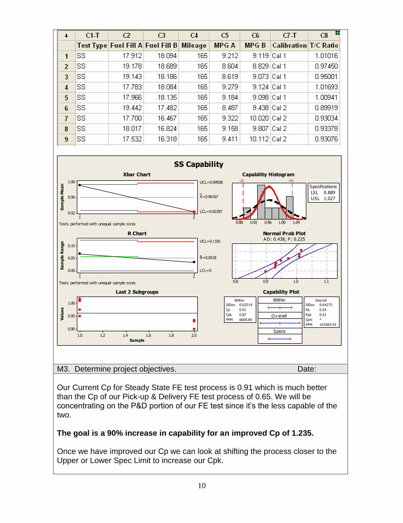
SS Capability

Xbar Chart


R Chart


Last 2 Subgroups



Capability Plot

M3. Determine project objectives. Date:

Our Current Cp for Steady State FE test process is 0.91 which is much better than the Cp of our Pick-up & Delivery FE test process of 0.65. We will be concentrating on the P&D portion of our FE test since it’s the less capable of the two. The goal is a 90% increase in capability for an improved Cp of 1.235. Once we have improved our Cp we can look at shifting the process closer to the Upper or Lower Spec Limit to increase our Cpk.

11

A1. Identify and list all potential causes (inputs). Date: 12/13/11 Required tools: Process map, Brainstorming, Fishbone diagram, FMEA, Cause and effect matrix, Potential “X” matrix

Effect

Truck Fuel

Driver Route

Tires/Tread

Vehicle Weight

Gear Ratio

Batteries

After Treatment

Driver

Temperature

Grade of Fuel

Braking

Shifting

Train ( hilly, flat)

Weather

Condition

Road Type

(Gravel, Concrete,

Asphalt)

Traffic

Construction

Acceleration

2% Efficiency

A2. Screen potential causes. Date: 12/7/11 Required tools: See A1

Screened through all input with test engineers to target key inputs for grading by Power Train Group. They will grade on a scale of 1 to 5. 1 = to no effect on Type 2 FE testing 2 = slight effect 3 = moderate effect 4 = great effect 5 = absolute effect Key inputs: Fuel Fill Method Driving Route Braking Techniques Acceleration Techniques Weather Conditions Vehicle Condition

12

A3. Determine the f(x) – key input variable(s) Date: 12/12/11 Required tools: Hypothesis testing, Correlation, Regression, Design of experiments Ran Chi-Square test to analysis the data collected.

*** Grade with an "X" the Key Inputs according

to their on Type II Fuel Economy Testing ***

No Slight Effect Moderate Grade Effect Absolute

Effect Effect Effect Effect Effect

1 2 3 4 5

Fuel Fill Method

Driving Route

BrakingTechniques

AccelerationTechniques

Weather conditions

Vehicle Condition

Key Inputs

GRADE CARD

13

A 4 2.7 4 3.95 4.5 2 1.9* 1 2.6 3 3.4

B 3 3.2 5 4.65 5.2 1 2.2 4 3.0 4 4.0

C 1 2.5 2 3.55 4.0 2 1.7* 3 2.3 4 3.1

D 1 2.7 5 3.92 4.5 3 1.9* 4 2.6 4 3.4

E 4 2.0 3 2.94 3.3 1 1.4* 1 1.9* 1 2.5

F 3 2.9 4 4.15 4.7 2 2.0* 2 2.7 4 3.6

Total 16 2326 11 15 20

Expected counts should be at least 2 to ensure the validity of the p-value for the test.

* Indicates a violation.

Obs Exp Obs ExpObs Exp Obs Exp Obs Exp Obs Exp

VehicleFuel Fill Route Braking Accelerating Weather

Observed and Expected Counts

Chi-Square Test for Association: Person by Factors

Diagnostic Report

association between Person and Factors.

significant (p < 0.05). You cannot conclude there is an

Differences among the outcome percentage profiles are not

> 0.50.10.050

NoYes

P = 0.974

Vehicle

Weather

Accelerating

Braking

Route

Fuel Fill

Average

30%20%10%0%

A

B

C

D

E

F

outcome percentage profiles at the 0.05 level of significance.

You cannot conclude that there are differences among the

Vehicle

Weather

Accelerating

Braking

Route

Fuel Fill

100%50%0%-50%-100%

A

B

C

D

E

F

17%13%

22%9%

22%17%

19%25%

6%6%

19%25%

20%5%

20%20%20%

15%

13%7%

27%20%

27%7%

18%9%

27%18%

9%18%

19%15%

8%19%19%19%

18%12%

18%15%

19%17%

Do the percentage profiles differ?

Percentage Profiles Chart

Compare the profiles.

Comments

Expected Counts

% Difference between Observed and

Positive: Occur more frequently than expected

Negative: Occur less frequently than expected

Chi-Square Test for Association: Person by Factors

Summary Report

14

VehicleWeatherAcceleratingBrakingRouteFuel Fill

6

5

4

3

2

1

Da

ta

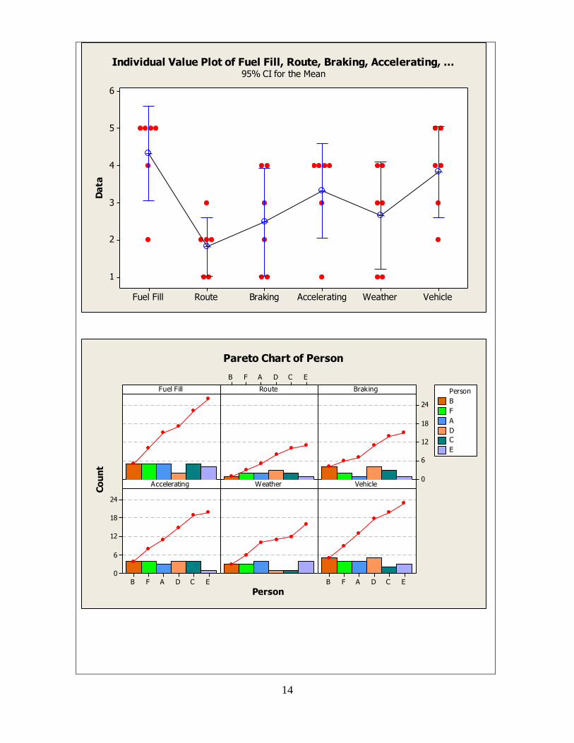
Individual Value Plot of Fuel Fill, Route, Braking, Accelerating, ...95% CI for the Mean

ECDAFB

24

18

12

6

0

ECDAFB

24

18

12

6

0ECDAFB

Fuel Fill

Person

Co

un

t

Route Braking

Accelerating Weather Vehicle

B

F

A

D

C

E

Person

Pareto Chart of Person

15

I-1. Establish operating tolerances for key inputs and the output. Date: 12/13/11 After examining the grade cards we found that Fuel Fill Technique seemed to be the input with the greatest effect on a FE test failure. Fuel weight tanks will be used in place of the OEM fuel tanks, Eliminating the Steve Stick & the variation associated with it. The trucks will be filled & left at the track for P&D testing to eliminate the variance associated with the trip to & from TDTC. Braking & Acceleration points will be set up on the track to remove a majority of the variation out of the driver’s techniques. Both Vehicles will be serviced & have new batteries installed to make their individual fuel economies more consistent. In addition to these changes, extra controls will be put into place for the Steady State & P&D Test.

16

New Process

Fuel Economy Testing

Six Sigma Project

November 18, 2011

Purge EDAQ and

Reset Trip -O-Meter

Remove & Weigh

Fuel Tanks.

Record Fuel used

& miles driven

1

2

3a

Fill Tanks,

Record Weights

& install on trucks

Trucks are parked

& fueled at IPG.

Trucks driven on

track per P&D.

Use Mileage from

GPS

Trucks Driven to

469 per trained

driving techniques.

Truck ran with

cruise at 55 mph.

Use Mileage from

GPS

P&D Steady StateP& D or Steady State

3b


4

17

I-2. Re-evaluate the measuring system. Date: 12/13/11 Required tools: Gage R&R/Attribute Agreement Analysis

Run Order Operators Parts Measurements

Run Order Operators Parts Measurements

1 Mike 200 200.1 25 Mike 100 100.1

2 Mike 50 50 26 Mike 200 200.1

3 Mike 100 100.1 27 Mike 50 50

4 Mike 25 25 28 Mike 25 25

5 Kirby 25 25 29 Kirby 25 25

6 Kirby 100 100 30 Kirby 100 100.1

7 Kirby 200 200.1 31 Kirby 50 50

8 Kirby 50 50 32 Kirby 200 200.1

9 Steve 100 100.1 33 Steve 25 25

10 Steve 25 25 34 Steve 100 100

11 Steve 200 200.1 35 Steve 200 200

12 Steve 50 50 36 Steve 50 50

13 Mike 50 50 37 Mike 200 200.1

14 Mike 25 25 38 Mike 25 25

15 Mike 200 200 39 Mike 100 100

16 Mike 100 100.1 40 Mike 50 50

17 Kirby 50 50 41 Kirby 50 50

18 Kirby 200 200.1 42 Kirby 200 200

19 Kirby 25 25 43 Kirby 25 25

20 Kirby 100 100 44 Kirby 100 100

21 Steve 200 200 45 Steve 50 50

22 Steve 50 50 46 Steve 100 100.1

23 Steve 100 100.1 47 Steve 25 25

24 Steve 25 25 48 Steve 200 200

18

200

100

0

Mike Kirby Steve

0.10

0.05

0.00

200

100

0

SteveKirbyMike

200

100

0

Variation Breakdown

Total Gage 0.038 0.05

Repeatability 0.035 0.05

Reproducibility 0.013 0.02

Part-to-Part 77.421 100.00

Process Var (data) 77.421 100.00

Source StDev (data)

%Process

Gage R&R Study for Measurements

Variation Report

Xbar Chart of Part Averages by Operator

At least 50% should be outside the limits. (actual: 100.0%)

R Chart of Test-Retest Ranges by Operator (Repeatability)

Operators and parts with larger ranges have less consistency.

Reproducibility — Operator by Part Interaction

Look for abnormal points or patterns.

Reproducibility — Operator Main Effects

Look for operators with higher or lower averages.

the parts in the study.

measurement system. The process variation is estimated from

0.0% of all process variation can be attributed to the

100%30%10%0%

NoYes

0.0%

ReproducibilityRepeatabilityTotal Gage

48

36

24

12

0

30

10

% of Process

the total variation in the process.

accounts for 34.9% of the measurement variation. It is 0.0% of

occurs when different people measure the same item. This

-- Operator component (Reproducibility): The variation that

is 0.0% of the total variation in the process.

times. This accounts for 93.7% of the measurement variation. It

occurs when the same person measures the same item multiple

-- Test-Retest component (Repeatability): The variation that

and use this information to guide improvements:

Examine the bar chart showing the component contributions,

>30%: unacceptable

10% - 30%: marginal

<10%: acceptable

General rules used to determine the capability of the system:

Number of parts in study 4

Number of operators in study 3

Number of replicates 4

Study Information

(Replicates: Number of times each operator measured each part)

Gage R&R Study for Measurements

Summary Report

Variation Breakdown

reproducibility?

Is there a problem with repeatability or

Comments

Can you adequately assess process performance?

19

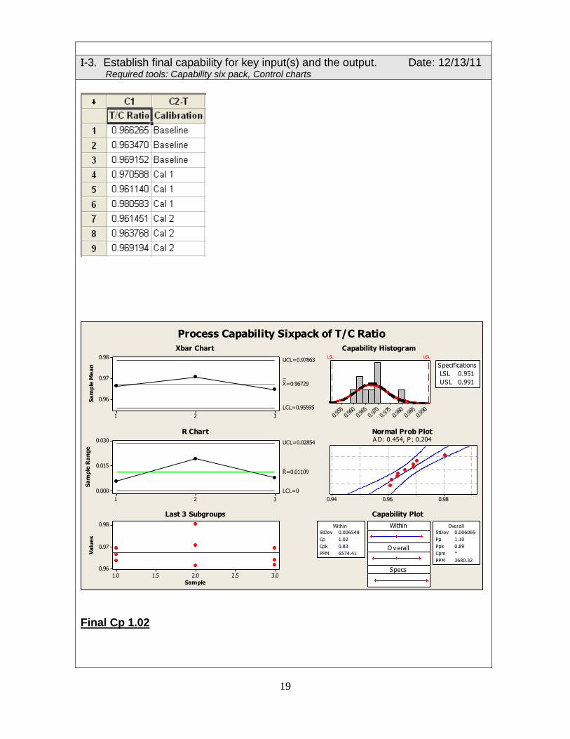
I-3. Establish final capability for key input(s) and the output. Date: 12/13/11 Required tools: Capability six pack, Control charts

321

0.98

0.97

0.96Sa

mp

le M

ea

n

__X=0.96729

UCL=0.97863

LCL=0.95595

321

0.030

0.015

0.000

Sa

mp

le R

an

ge

_R=0.01109

UCL=0.02854

LCL=0

3.02.52.01.51.0

0.98

0.97

0.96

Sample

Va

lue

s

0.99

00.98

50.98

00.975

0.970

0.96

50.96

00.95

5

LSL USL

LSL 0.951

USL 0.991

Specifications

0.980.960.94

Within

O v erall

Specs

StDev 0.006548

Cp 1.02

Cpk 0.83

PPM 6574.41

Within

StDev 0.006069

Pp 1.10

Ppk 0.89

Cpm *

PPM 3680.32

Overall

Process Capability Sixpack of T/C Ratio

Xbar Chart

R Chart

Last 3 Subgroups



Capability Plot

Final Cp 1.02

20

C1. Implement process controls for the key inputs. Date:12/13/11 Required tool: Error proofing

List controls including error proofing. Utilize highest level of control possible. Categorize controls 0, 1, 2, or 3.

Drivers ---Driving Habits (Insert controls (Training)) WOT Till- 5 mph of posted speed limits Coast & Braking same Distance Cruise set for same time (Steady State SS Only) Synchronized Lane changes Level 1 control Drivers/ Engineer --- (Use satellite mileage) Miles are set according to course or route. Too much variation on track when other test is being ran at the same time ( using different lanes which vary in length per lap) Unscheduled but necessary stops on SS route add miles. Both Speedometers have been Calibrated! Level 2 control Truck Maintenance--- (installed new Batteries) Old methods= Bad Batteries Alternators would have to recharge batteries after truck sat. Varied on length of time the truck sat. Extra hp needed = more fuel New method= Test to be ran with both trucks running the same accessories through out the entire FE test Level 1 & 2 control

Follow-up to ensure effectiveness. Date:

No wasted runs as of yet but we’ve only had 9 runs. Note: Describe justification(s) for omitting any of the above steps, or required tools.

Black Belt Six Sigma Project Summary - Faculty...

Documents

Transcript of Black Belt Six Sigma Project Summary - Faculty...