Bjork - Ch 4 Differential_Equations

of 27 Stochastic Integrals

PRINTED FROM OXFORD SCHOLARSHIP ONLINE (www.oxfordscholarship.com). (c) Copyright Oxford University Press, 2013.All Rights Reserved. Under the terms of the licence agreement, an individual user may print out a PDF of a single chapter of amonograph in OSO for personal use (for details see http://www.oxfordscholarship.com/page/privacy-policy). Subscriber: ColumbiaUniversity; date: 21 February 2013

Arbitrage Theory in Continuous TimeTomas Björk

Print publication date: 2004Print ISBN-13: 9780199271269Published to Oxford Scholarship Online: Oct-05DOI: 10.1093/0199271267.001.0001

Stochastic Integrals

Tomas Björk (Contributor Webpage)

DOI: 10.1093/0199271267.003.0004

Abstract and Keywords

This chapter discusses the modelling of asset prices as continuous timestochastic processes. Diffusion processes and stochastic differentialequations are used as building blocks to obtain the most complete andelegant theory. Practice exercises are included.

Keywords: asset prices, stochastic processes, diffusion processes, differential equations,continuous time

4.1 Introduction

The purpose of this book is to study asset pricing on financial markets incontinuous time. We thus want to model asset prices as continuous timestochastic processes, and the most complete and elegant theory is obtainedif we use diffusion processes and stochastic differential equations asour building blocks. What, then, is a diffusion?

Loosely speaking we say that a stochastic process X is a diffusiondiffusion ifits local dynamics can be approximated by a stochastic difference equationof the following type:

Here Z(t) is a normally distributed disturbance term which is independentof everything which has happened up to time t, while μ and σ are givendeterministic functions. The intuitive content of (4.1) is that, over the timeinterval [t, t + Δ t], the X-process is driven by two separate terms.

http://www.oxfordscholarship.com/page/privacy-policy

http://www.oxfordscholarship.com/view/10.1093/0199271267.001.0001/acprof-9780199271269-chapter-4#acprof-9780199271269-displayMaths-113



• A locally deterministic velocity μ (t, X(t)).• A Gaussian disturbance term, amplified by the factor σ (t, X(t)).

The function μ is called the (local) drift term term of the process, whereasσ is called the diffusion term term. In order to model the Gaussiandisturbance terms we need the concept of a Wiener process.

Definition 4.1 A stochastic process W is called a Wiener process if thefollowing conditions hold:

1 W(0) = 0.2 The process W has independent increments, i.e. if r < s ≤ t <u then W(u) − W(t) and W(s) − W(r) are independent stochasticvariables.3 For s < t the stochastic variable W(t) − W(s) has the Gaussiandistribution

.3 W has continuous trajectories.

Remark 4.1.1 Note that we use a somewhat old fashioned notation, whereN [μ, σ] denotes a Gaussian distribution with expected value μ and standarddeviation σ.

In Fig. 4.1 a computer simulated Wiener trajectory is shown.

Fig. 4.1. A Wiener trajectory




(p. 37 )

We may now use a Wiener process in order to write (4.1) as

where Δ W(t) is defined by

Let us now try to make (4.2) a bit more precise. It is then tempting to dividethe equation by Δt and let Δt tend to zero. Formally, we would obtain

where we have added an initial condition and where

is the formal time derivative of the Wiener process W.

If v were an ordinary (and well defined) process we would now in principlebe able to solve (4.3) as a standard ordinary differential equation (ODE) for (p. 38 ) each v-trajectory. However, it can be shown that with probability 1a Wiener trajectory is nowhere differentiable (cf. Fig. 4.1), so the process vcannot even be defined. Thus this is a dead end.

Another possibility of making eqn (4.2) more precise is to let Δt tend to zerowithout first dividing the equation by Δt. Formally we will then obtain theexpression

and it is now natural to interpret (4.5) as a shorthand version of the followingintegral equation

In eqn (4.6) we may interpret the ds-integral as an ordinary Riemannintegral. The natural interpretation of the dW-integral is to view it as aRiemann–Stieltjes integral for each W-trajectory, but unfortunately this is notpossible since one can show that the W-trajectories are of locally unboundedvariation. Thus the stochastic dW-integral cannot be defined in a naive way.

As long as we insist on giving a precise meaning to eqn (4.2) for each W-trajectory separately, we thus seem to be in a hopeless situation. If,however, we relax our demand that the dW-integral in eqn (4.6) should bedefined trajectorywise we can still proceed. It is in fact possible to give aglobal (L2-)definition of integrals of the form












for a large class of processes g. This new integral concept—the so called Itôintegral—will then give rise to a very powerful type of stochastic differentialcalculus—the Itô calculus. Our program for the future thus consists of thefollowing steps:

1 Define integrals of the type

.2 Develop the corresponding differential calculus.3 Analyze stochastic differential equations of the type (4.5) usingthe stochastic calculus above.

4.2 Information

Let X be any given stochastic process. In the sequel it will be important todefine “the information generated by X” as time goes by. To do this in arigorous (p. 39 ) fashion is outside the main scope of this book, but for mostpractical purposes the following heuristic definitions will do nicely. See theappendices for a precise treatment.

Definition 4.2 The symbol

denotes “the information generated by X on the interval [0, t]”, oralternatively “what has happened to X over the interval [0, t]”. If, basedupon observations of the trajectory {X(s); 0 ≤ s ≤ t}, it is possible to decidewhether a given event A has occurred or not, then we write this as

or say that “A is

-measurable”.

If the value of a given stochastic variable Z can be completely determinedgiven observations of the trajectory {X(s); 0 ≤ s ≤ t}, then we also write

If Y is a stochastic process such that we have

for all t ≥ 0 then we say that Y is adapted to the filtration





.

The above definition is only intended to have an intuitive content, since aprecise definition would take us into the realm of abstract measure theory.Nevertheless it is usually extremely simple to use the definition, and we nowgive some fairly typical examples.

1 If we define the event A by A = {X(s) ≤ 3.14, for all s ≤ 9} thenwe have

.2 For the event A = {X(10) > 8} we have

. Note, however, that we do not have

, since it is impossible to decide if A has occurred or not on thebasis of having observed the X-trajectory only over the interval [0,9].3 For the stochastic variable Z, defined by

we have

.4 If W is a Wiener process and if the process X is defined by

then X is adapted to the W-filtration.• (p. 40 )

5 With W as above, but with X defined as

X is not adapted (to the W-filtration).

4.3 Stochastic Integrals

We now turn to the construction of the stochastic integral. For that purposewe consider as given a Wiener process W, and another stochastic processg. In order to guarantee the existence of the stochastic integral we have to




impose some kind of integrability conditions on g, and the class £2 turns outto be natural.

Definition 4.3

(i) We say that the process g belongs to the class £2 [a, b] if thefollowing conditions are satisfied.

• •

.• • The process g is adapted to the

-filtration.(ii) We say that the process g belongs to the class £2 if g ∈ £2 [0, t]for all t > 0.

Our object is now to define the stochastic integral

, for a process g ∈ £2 [a, b], and this is carried out in two steps.

Suppose to begin with that the process g ∈ £2 [a, b] is simple, i.e. that thereexist deterministic points in time a = t0 < t1 < … < tn = b, such that g isconstant on each subinterval. In other words we assume that g(s) = g(tk) fors ∈ [tk, tk + 1). Then we define the stochastic integral by the obvious formula

Remark 4.3.1 Note that in the definition of the stochastic integral we takeso called forward increments of the Wiener process. More specifically, in thegeneric term g(tk) [W(tk + 1) − W(tk)] of the sum the process g is evaluated atthe left end tk of the interval [tk, tk + 1] over which we take the W-increment.This is essential to the following theory both from a mathematical and (as weshall see later) from an economical point of view.

For a general process g ∈ £2 [a, b] which is not simple we may schematicallyproceed as follows:

1 Approximate g with a sequence of simple processes gn such that




• (p. 41 )2 For each n the integral

is a well-defined stochastic variable Zn, and it is possible to provethat there exists a stochastic variable Z such that Zn → Z (in L2) asn → ∞.3 We now define the stochastic integral by

The most important properties of the stochastic integral are given by thefollowing proposition. In particular we will use the property (4.12) over andover again.

Proposition 4.4 Let g be a process satisfying the conditions

Then the following relations hold:

Proof A full proof is outside the scope of this book, but the general strategyis to start by proving all the assertions above in the case when g is simple.This is fairly easily done, and then it “only” remains to go to the limit in thesense of (4.9). We illustrate the technique by proving (4.12) in the case of asimple g. We obtain

Since g is adapted, the value g(tk) only depends on the behavior of theWiener process on the interval [0, tk]. Now, by definition W has independent







increments, so [W(tk + 1)) − W(tk)] (which is a forward increment) isindependent of g(tk). (p. 42 ) Thus we have

□

Remark 4.3.2 It is possible to define the stochastic integral for a process gsatisfying only the weak condition

For such a general g we have no guarantee that the properties (4.12) and(4.13) hold. Property (4.14) is, however, still valid.

4.4 Martingales

The theory of stochastic integration is intimately connected to the theory ofmartingales, and the modern theory of financial derivatives is in fact basedmainly on martingale theory. Martingale theory, however, requires somebasic knowledge of abstract measure theory, and a formal treatment is thusoutside the scope of the more elementary parts of this book.

Because of its great importance for the field, however, it would beunreasonable to pass over this important topic entirely, and the object ofthis section is to (informally) introduce the martingale concept. The moreadvanced reader is referred to the appendices for details.

Let us therefore consider a given filtration (“flow of information”) {ℱt}t≥0,where, as before, the reader can think of ℱt as the information generated byall observed events up to time t. For any stochastic variable Y we now let thesymbol

denote the “expected value of Y, given the information available at time t”.A precise definition of this object requires measure theory, so we have tobe content with this informal description. Note that for a fixed t, the objectE[Y∣ℱt] is a stochastic variable. If, for example, the filtration is generatedby a single observed process X, then the information available at time twill of course depend upon the behavior of X over the interval [0, t], so theconditional expectation E[Y∣ℱt] will in this case be a function of all past X-values {X(s): s ≤ t}. We will need the following two rules of calculation.







Proposition 4.5

• If Y and Z are stochastic variables, and Z is ℱt-measurable, then

• (p. 43 )• If Y is a stochastic variable, and if s < t, then

The first of these results should be obvious: in the expected value E[Z · Y∣ℱt]we condition upon all information available time t. If now Z ∈ ℱt, this meansthat, given the information ℱt, we know exactly the value of Z, so in theconditional expectation Z can be treated as a constant, and thus it can betaken outside the expectation. The second result is called the “law of iteratedexpectations”, and it is basically a version of the law of total probability.

We can now define the martingale concept.

Definition 4.6 A stochastic process X is called an (ℱt)-martingale if thefollowing conditions hold:

• X is adapted to the filtration {ℱ}t≥0.• For all t

• For all s and t with s ≤ t the following relation holds:

A process satisfying, for all s and t with s ≤ t, the inequality

is called a supermartingale, and a process satisfying

is called a submartingale.

The first condition says that we can observe the value X(t) at time t, and thesecond condition is just a technical condition. The really important conditionis the third one, which says that the expectation of a future value of X, giventhe information available today, equals today's observed value of X. Anotherway of putting this is to say that a martingale has no systematic drift.

It is possible to prove the following extension of Proposition 4.4.




Proposition 4.7 For any process g ∈ £2 [s, t] the following hold:

As a corollary we obtain the following important fact.

(p. 44 ) Corollary 4.8 For any process g ∈ £2, the process X, defined by

is an

-martingale. In other words, modulo an integrability condition, everystochastic integral is a martingale.

Proof Fix s and t with s < t. We have

The integral in the first expectation is, by Proposition 4.4, measurable w.r.t.

, so by Proposition 4.5 we have

From Proposition 4.4 we also see that

, so we obtain

□

We have in fact the following stronger (and very useful) result.

Lemma 4.9 Within the framework above, and assuming enoughintegrability, a stochastic process X (having a stochastic differential) is amartingale if and only if the stochastic differential has the form

i.e. X has no dt-term.

Proof We have already seen that if dX has no dt-term then X is a martingale.The reverse implication is much harder to prove, and the reader is referredto the literature cited in the notes below.□




(p. 45 ) 4.5 Stochastic Calculus and the Itô Formula

Let X be a stochastic process and suppose that there exists a real number x0and two adapted processes μ and σ such that the following relation holds forall t ≥ 0.

where a is some given real number. As usual W is a Wiener process. To usea less cumbersome notation we will often write eqn (4.16) in the followingform:

In this case we say that X has a stochastic differential given by (4.17)with an initial condition given by (4.18). Note that the formal string dX(t)= μ(t) dt + σ(t) dW(t) has no independent meaning. It is simply a shorthandversion of the expression (4.16) above. From an intuitive point of view thestochastic differential is, however, a much more natural object to considerthan the corresponding integral expression. This is because the stochasticdifferential gives us the “infinitesimal dynamics” of the X-process, and as wehave seen in Section 4.1, both the drift term μ (s) and the diffusion term σ(s)have a natural intuitive interpretation.

Let us assume that X indeed has the stochastic differential above. Looselyspeaking we thus see that the infinitesimal increment dX(t) consists of alocally deterministic drift term μ(t) dt plus an additive Gaussian noise termσ(t) dW(t). Assume furthermore that we are given a C1,2-function

and let us now define a new process Z by

We may now ask what the local dynamics of the Z-process look like, and atfirst it seems fairly obvious that, except for the case when f is linear in x,Z will not have a stochastic differential. Consider, for example, a discretetime example where X satisfies a stochastic difference equation with additiveGaussian noise in each step, and suppose that f(t, x) = ex. Then it is clearthat Z will not be driven by additive Gaussian noise—the noise will in fact bemultiplicative and log-normal. It is therefore extremely surprising that forcontinuous time models the stochastic differential structure with a drift termplus additive Gaussian noise will in fact be preserved even under nonlineartransformations. Thus the process Z will have a stochastic differential, andthe form of dZ is given explicitly by the famous (p. 46 ) Itô formula below.






http://www.oxfordscholarship.com/view/10.1093/0199271267.001.0001/acprof-9780199271269-chapter-4#acprof-9780199271269-div1-12



Before turning to the Itô formula we have to take a closer look at somerather fine properties of the trajectories of the Wiener process.

As we saw earlier the Wiener process is defined by a number of very simpleprobabilistic properties. It is therefore natural to assume that a typicalWiener trajectory is a fairly simple object, but this is not at all the case. Onthe contrary—one can show that, with probability 1, the Wiener trajectorywill be a continuous function of time (see the definition above) which isnondifferentiable at every point. Thus a typical trajectory is a continuouscurve consisting entirely of corners and it is of course quite impossible todraw a figure of such an object (it is in fact fairly hard to prove that such acurve actually exists). This lack of smoothness gives rise to an odd propertyof the quadratic variation of the Wiener trajectory, and since the entiretheory to follow depends on this particular property we now take some timeto study the Wiener increments a bit closer.

Let us therefore fix two points in time, s and t with s < t, and let us use thehandy notation

Using well-known properties of the normal distribution it is fairly easy toobtain the following results, which we will use frequently

We see that the squared Wiener increment (ΔW(t))2 has an expected valuewhich equals the time increment Δt. The really important fact, however, isthat, according to (4.22), the variance of [ΔW(t)]2 is negligible compared toits expected value. In other words, as Δt tends to zero [ΔW(t)]2 will of coursealso tend to zero, but the variance will approach zero much faster than theexpected value. Thus [ΔW(t)]2 will look more and more “deterministic” andwe are led to believe that in the limit we have the purely formal equality

The reasoning above is purely heuristic. It requires a lot of hard work toturn the relation (4.23) into a mathematically precise statement, and itis of course even harder to prove it. We will not attempt either a preciseformulation or a precise proof. In order to give the reader a flavor of the fulltheory we will, however, give another argument for the relation (4.23).







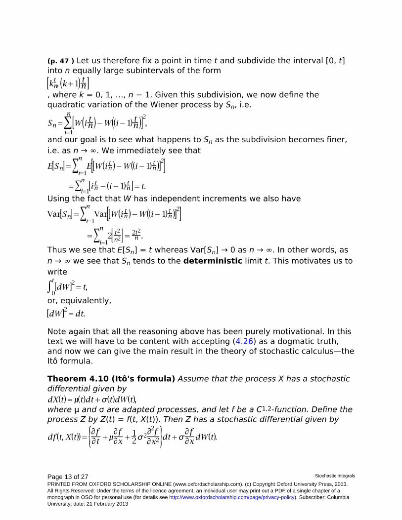
(p. 47 ) Let us therefore fix a point in time t and subdivide the interval [0, t]into n equally large subintervals of the form

, where k = 0, 1, …, n − 1. Given this subdivision, we now define thequadratic variation of the Wiener process by Sn, i.e.

and our goal is to see what happens to Sn as the subdivision becomes finer,i.e. as n → ∞. We immediately see that

Using the fact that W has independent increments we also have

Thus we see that E[Sn] = t whereas Var[Sn] → 0 as n → ∞. In other words, asn → ∞ we see that Sn tends to the deterministic limit t. This motivates us towrite

or, equivalently,

Note again that all the reasoning above has been purely motivational. In thistext we will have to be content with accepting (4.26) as a dogmatic truth,and now we can give the main result in the theory of stochastic calculus—theItô formula.

Theorem 4.10 (Itô's formula) Assume that the process X has a stochasticdifferential given by

where μ and σ are adapted processes, and let f be a C1,2-function. Define theprocess Z by Z(t) = f(t, X(t)). Then Z has a stochastic differential given by





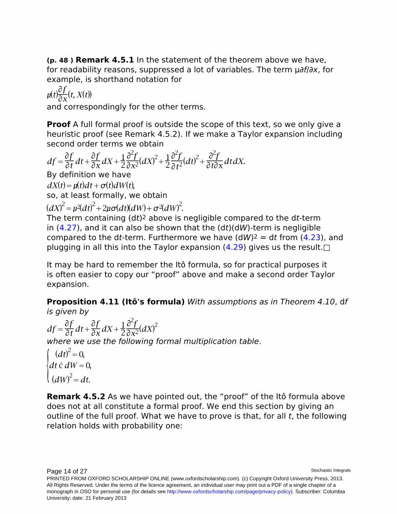
(p. 48 ) Remark 4.5.1 In the statement of the theorem above we have,for readability reasons, suppressed a lot of variables. The term μ∂f/∂x, forexample, is shorthand notation for

and correspondingly for the other terms.

Proof A full formal proof is outside the scope of this text, so we only give aheuristic proof (see Remark 4.5.2). If we make a Taylor expansion includingsecond order terms we obtain

By definition we have

so, at least formally, we obtain

The term containing (dt)2 above is negligible compared to the dt-termin (4.27), and it can also be shown that the (dt)(dW)-term is negligiblecompared to the dt-term. Furthermore we have (dW)2 = dt from (4.23), andplugging in all this into the Taylor expansion (4.29) gives us the result.□

It may be hard to remember the Itô formula, so for practical purposes itis often easier to copy our “proof” above and make a second order Taylorexpansion.

Proposition 4.11 (Itô's formula) With assumptions as in Theorem 4.10, dfis given by

where we use the following formal multiplication table.

Remark 4.5.2 As we have pointed out, the “proof” of the Itô formula abovedoes not at all constitute a formal proof. We end this section by giving anoutline of the full proof. What we have to prove is that, for all t, the followingrelation holds with probability one:







(p. 49 ) We therefore divide the interval [0, t] as 0 = t0 < t1 < … < tn = t inton equal subintervals. Then we have

Using Taylor's formula we obtain, with subscripts denoting partial derivativesand obvious notation,

where Qk is the remainder term. Furthermore, we have

where Sk is a remainder term. From this we obtain

where Pk is a remainder term. If we now substitute (4.33)–(4.35) into (4.32)we obtain, in shorthand notation,

where

Letting n → ∞ we have, more or less by definition,

Very much as when we proved earlier that Σ (ΔWk)2 → t, it is possible to showthat







(p. 50 ) and it is fairly easy to show that K1 and K2 converge to zero. Thereally hard part is to show that the term R, which is a large sum of individualremainder terms, also converges to zero. This can, however, also be doneand the proof is finished.

4.6 Examples

In order to illustrate the use of the Itô formula we now give some examples.All these examples are quite simple, and the results could have beenobtained as well by using standard techniques from elementary probabilitytheory. The full force of the Itô calculus will be seen in the following chapters.

The first two examples illustrate a useful technique for computing expectedvalues in situations involving Wiener processes. Since arbitrage pricing to alarge extent consists of precisely the computation of certain expected valuesthis technique will be used repeatedly in the sequel.

Suppose that we want to compute the expected value E[Y] where Y is somestochastic variable. Schematically we will then proceed as follows:

1 Try to write Y as Y = Z(t0) where t0 is some point in time and Z isa stochastic process having an Itô differential.2 Use the Itô formula to compute dZ as, for example,

3 Write this expression in integrated form as

4 Take expected values. Using Proposition 4.4 we see that thedW-integral will vanish. For the ds-integral we may move theexpectation operator inside the integral sign (an integral is “just” asum), and we thus have

Now two cases can occur:

• (a) We may, by skill or pure luck, be able to calculate the expected valueE[μ(s)] explicitly. Then we only have to compute an ordinary Riemannintegral to obtain E[Z(t)], and thus to read off E[Y] = E[Z(t0)].




• (b) If we cannot compute E[μ(s)] directly we have a harder problem, but insome cases we may convert our problem to that of solving an ODE.

(p. 51 ) Example 4.12 Compute E[W4(t)].

Solution: Define Z by Z(t) = W4(t). Then we have Z(t) = f(t, X(t)) where X =W and f is given by f(t, x) = x4. Thus the stochastic differential of X is trivial,namely dX = dW, which, in the notation of the Itô formula (4.28), means thatμ = 0 and σ = 1. Furthermore we have ∂f/∂t = 0, ∂f/∂x = 4x3, and ∂2 f/∂ x2 =12x2. Thus the Itô formula gives us

Written in integral form this reads

Now we take the expected values of both members of this expression. Then,by Proposition 4.4, the stochastic integral will vanish. Furthermore we maymove the expectation operator inside the ds-integral, so we obtain

Now we recall that E[W2(s)] = s, so in the end we have our desired result

□

Example 4.13 Compute E[eαW(t)].

Solution: Define Z by Z(t) = eαW(t). The Itô formula gives us

so we see that Z satisfies the stochastic differential equation (SDE)

In integral form this reads

(p. 52 ) Taking expected values will make the stochastic integral vanish.After moving the expectation within the integral sign in the ds-integral anddefining m by m(t) = E[Z(t)] we obtain the equation





This is an integral equation, but if we take the t-derivative we obtain the ODE

Solving this standard equation gives us the answer

□

It is natural to ask whether one can “compute” (in some sense) the value of astochastic integral. This is a fairly vague question, but regardless of how it isinterpreted, the answer is generally no. There are just a few examples wherethe stochastic integral can be computed in a fairly explicit way. Here is themost famous one.

Example 4.14 Compute

Solution: A natural guess is perhaps that

. Since Itô calculus does not coincide with ordinary calculus this guess cannotpossibly be true, but nevertheless it seems natural to start by investigatingthe process Z(t) = W2(t). Using the Itô formula on the function f(t, x) = x2

and with X = W we get

In integrated form this reads

so we get our answer

□

We end with a useful lemma.

(p. 53 ) Lemma 4.15 Let σ (t) be a given deterministic function of time anddefine the process X by

Then X(t) has a normal distribution with zero mean, and variance given by




This is of course an expected result because the integral is “just” a linearcombination of the normally distributed Wiener increments with deterministiccoefficients. See the exercises for a hint of the proof.

4.7 The Multidimensional Itô Formula

Let us now consider a vector process X = (X1, …, Xn)*, where the componentXi has a stochastic differential of the form

and W1, …, Wd are d independent Wiener processes.

Defining the drift vector μ by

the d-dimensional vector Wiener process W by

and the n × d-dimensional diffusion matrix σ by

we may write the X-dynamics as

(p. 54 ) Let us furthermore define the process Z by

where f:R+ × Rn → R is a C1, 2 mapping. Then, using arguments as above, itcan be shown that the stochastic differential df is given by

with the extended multiplication rule (see the exercises)




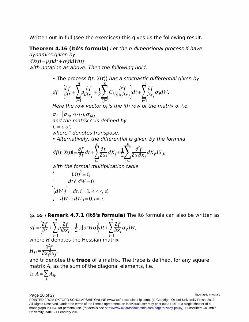
Written out in full (see the exercises) this gives us the following result.

Theorem 4.16 (Itô's formula) Let the n-dimensional process X havedynamics given by

with notation as above. Then the following hold:

• The process f(t, X(t)) has a stochastic differential given by

Here the row vector σi is the ith row of the matrix σ, i.e.

and the matrix C is defined by

where * denotes transpose.• Alternatively, the differential is given by the formula

with the formal multiplication table

(p. 55 ) Remark 4.7.1 (Itô's formula) The Itô formula can also be written as

where H denotes the Hessian matrix

and tr denotes the trace of a matrix. The trace is defined, for any squarematrix A, as the sum of the diagonal elements, i.e.




See the exercises for details.

4.8 Correlated Wiener Processes

Up to this point we have only considered independent Wiener processes, butsometimes it is convenient to build models based upon Wiener processeswhich are correlated. In order to define such objects, let us thereforeconsider d independent standard (i.e. unit variance) Wiener processes

. Let furthermore a (deterministic and constant) matrix

be given, and consider the n-dimensional processes W, defined by

where

In other words

(p. 56 ) Let us now assume that the rows of δ have unit length, i.e.

where the Euclidean norm is defined as usual by

Then it is easy to see (how?) that each of the components W1, …, Wnseparately are standard (i.e. unit variance) Wiener processes. Let us nowdefine the (instantaneous) correlation matrix ρ of W by

We then obtain




i.e.

Definition 4.17 The process W, constructed as above, is called a vector ofcorrelated Wiener processes, with correlation matrix ρ.

Using this definition we have the following Itô formula for correlated Wienerprocesses.

Proposition 4.18 (Itô's formula) Take a vector Wiener process W =(W1, …, Wn) with correlation matrix ρ as given, and assume that the vectorprocess X = (X1, …, Xk)* has a stochastic differential. Then the following hold:

• For any C1,2 function f, the stochastic differential of the processf(t, X(t)) is given by

(p. 57 ) with the formal multiplication table

• If, in particular, k = n and dX has the structure

where μ1, …, μn and σ1, …, σn are scalar processes, then thestochastic differential of the process f(t, X(t)) is given by

We end this section by showing how it is possible to translate between thetwo formalisms above. Suppose therefore that the n-dimensional process Xhas a stochastic differential of the form

i.e.

Thus the drift vector process μ is given by




and the diffusion matrix process σ by

W is assumed to be d-dimensional standard vector Wiener process (i.e. withindependent components) of the form

(p. 58 ) The system (4.38) can also be written as

where, as usual, σi is the ith row of the matrix σ. Let us now define n newscalar Wiener processes

by

We can then write the X-dynamics as

As is easily seen, each

is a standard scalar Wiener process, but

are of course correlated. The local correlation is easily calculated as

Summing up we have the following result.

Proposition 4.19 The system

where W1, …, Wd are independent, may equivalently be written as

where





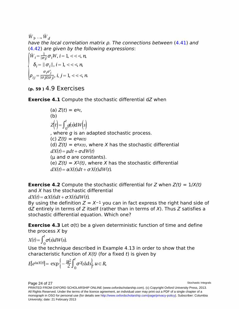
have the local correlation matrix ρ. The connections between (4.41) and(4.42) are given by the following expressions:

(p. 59 ) 4.9 Exercises

Exercise 4.1 Compute the stochastic differential dZ when

(a) Z(t) = eαt,(b)

, where g is an adapted stochastic process.(c) Z(t) = eαW(t)(d) Z(t) = eαX(t), where X has the stochastic differential

(μ and σ are constants).(e) Z(t) = X2(t), where X has the stochastic differential

Exercise 4.2 Compute the stochastic differential for Z when Z(t) = 1/X(t)and X has the stochastic differential

By using the definition Z = X−1 you can in fact express the right hand side ofdZ entirely in terms of Z itself (rather than in terms of X). Thus Z satisfies astochastic differential equation. Which one?

Exercise 4.3 Let σ(t) be a given deterministic function of time and definethe process X by

Use the technique described in Example 4.13 in order to show that thecharacteristic function of X(t) (for a fixed t) is given by






thus showing that X(t) is normally distributed with zero mean and a variancegiven by

Exercise 4.4 Suppose that X has the stochastic differential

where α is a real number whereas σ(t) is any stochastic process. Use thetechnique in Example 4.13 in order to determine the function m(t) = E[X(t)].

(p. 60 ) Exercise 4.5 Suppose that the process X has a stochastic differential

and that μ(t) ≥ 0 with probability one for all t. Show that this implies that X isa submartingale.

Exercise 4.6 A function h(x1, …, xn) is said to be harmonic if it satisfies thecondition

It is subharmonic if it satisfies the condition

Let W1, …, Wn be independent standard Wiener processes, and definethe process X by X(t) = h(W1(t), …, Wn(t)). Show that X is a martingale(submartingale) if h is harmonic (subharmonic).

Exercise 4.7 The object of this exercise is to give an argument for theformal identity

when W1 and W2 are independent Wiener processes. Let us therefore fix atime t, and divide the interval [0, t] into equidistant points 0 = t0 < t1 < … <tn = t, where

. We use the notation

Now define Qn by




Show that Qn → 0 in L2, i.e. show that

Exercise 4.8 Let X and Y be given as the solutions to the following system ofstochastic differential equations.

(p. 61 ) Note that the initial values x0, y0 are deterministic constants.

(a) Prove that the process R defined by R(t) = X2 (t) + Y2(t) isdeterministic.[(b)] Compute E[X(t)].

Exercise 4.9 For a n × n matrix A, the trace of a matrix of A is defined as

(a) If B is n × d and C is d × n, then BC is n × n. Show that

(b) With assumptions as above, show that

(c) Show that the Itô formula in Theorem 4.16 can be written as

where H denotes the HessianHessian matrix

Exercise 4.10 Prove all claims in Section 4.8.


http://www.oxfordscholarship.com/view/10.1093/0199271267.001.0001/acprof-9780199271269-chapter-4#acprof-9780199271269-div1-19



4.10 Notes

As a (far reaching) introduction to stochastic calculus and its applications,Øksendal (1995) and Steele (2001) can be recommended. Standardreferences on a more advanced level are Karatzas and Shreve (1988), andRevuz and Yor (1991). The theory of stochastic integration can be extendedfrom the Wiener framework to allow for semimartingales as integrators,and a classic in this field is Meyer (1976). Standard references are Jacodand Shiryaev (1987), Elliott (1982), and Dellacherie and Meyer (1972). Analternative to the classic approach to semimartingale integration theory ispresented in Protter (1990).


http://www.oxfordscholarship.com/view/10.1093/0199271267.001.0001/acprof-9780199271269-bibliography-1#acprof-9780199271269-bibItem-123









Bjork - Ch 4 Differential_Equations

Documents

Transcript of Bjork - Ch 4 Differential_Equations