BIZ2121-04 Production & Operations...
53
BIZ2121-04 Production & Operations Management Process Capacity Sung Joo Bae, Assistant Professor Yonsei University School of Business
-
Upload
nguyentram -
Category
Documents
-
view
226 -
download
0
Transcript of BIZ2121-04 Production & Operations...
BIZ2121-04 Production & Operations Management
Process Capacity
Sung Joo Bae, Assistant Professor
Yonsei University School of Business

Sharp’s Capacity Problem
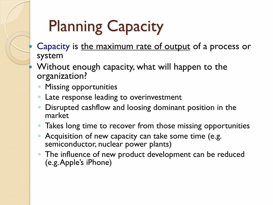
Planning Capacity Capacity is the maximum rate of output of a process or
system
Without enough capacity, what will happen to the organization? ◦ Missing opportunities
◦ Late response leading to overinvestment
◦ Disrupted cashflow and loosing dominant position in the market
◦ Takes long time to recover from those missing opportunities
◦ Acquisition of new capacity can take some time (e.g. semiconductor, nuclear power plants)
◦ The influence of new product development can be reduced (e.g. Apple’s iPhone)
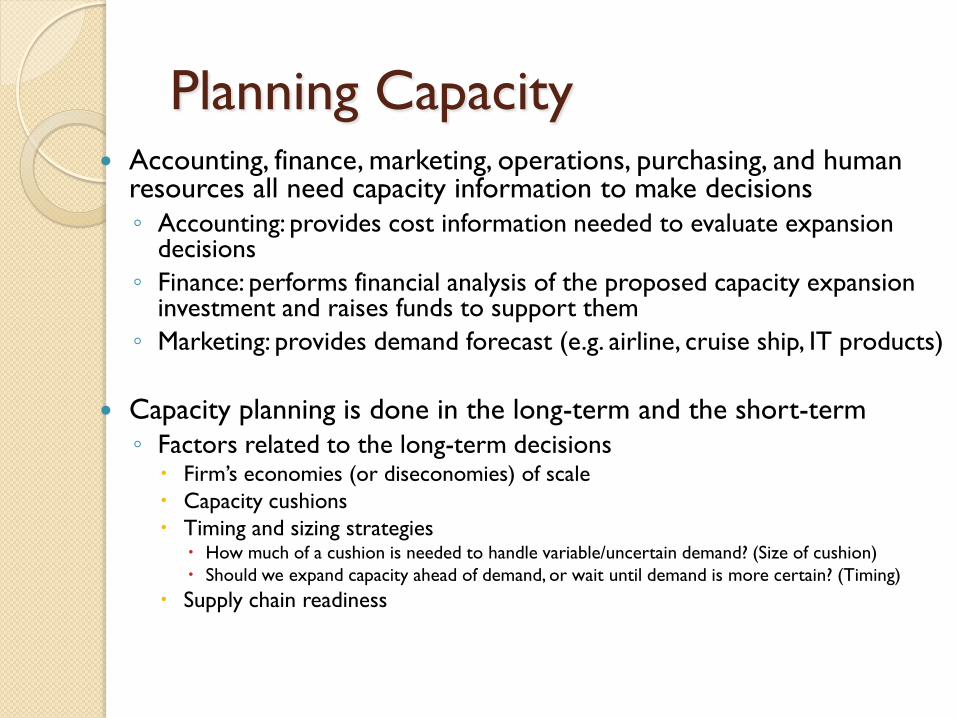
Planning Capacity Accounting, finance, marketing, operations, purchasing, and human
resources all need capacity information to make decisions
◦ Accounting: provides cost information needed to evaluate expansion decisions
◦ Finance: performs financial analysis of the proposed capacity expansion investment and raises funds to support them
◦ Marketing: provides demand forecast (e.g. airline, cruise ship, IT products)
Capacity planning is done in the long-term and the short-term
◦ Factors related to the long-term decisions Firm’s economies (or diseconomies) of scale
Capacity cushions
Timing and sizing strategies How much of a cushion is needed to handle variable/uncertain demand? (Size of cushion)
Should we expand capacity ahead of demand, or wait until demand is more certain? (Timing)
Supply chain readiness
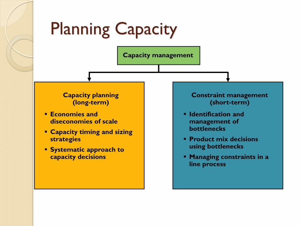
Planning Capacity
Capacity planning (long-term)
Economies and diseconomies of scale
Capacity timing and sizing strategies
Systematic approach to capacity decisions
Constraint management (short-term)
Identification and management of bottlenecks
Product mix decisions using bottlenecks
Managing constraints in a line process
Capacity management
Measures of Capacity Utilization
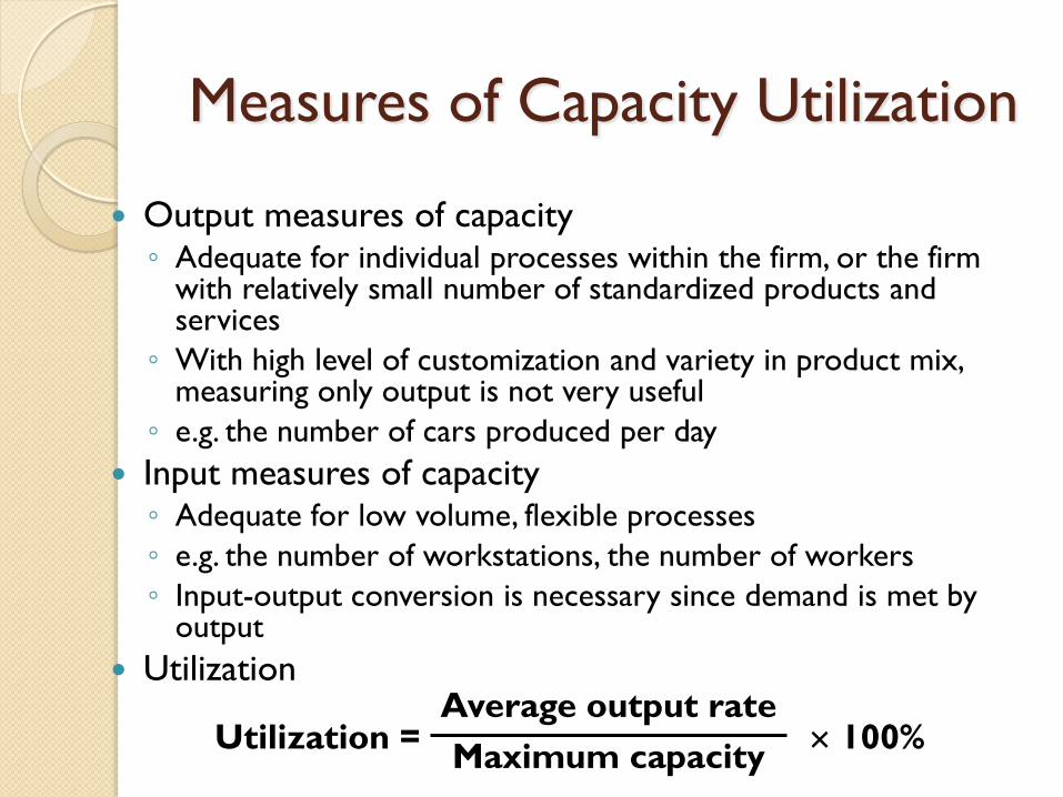
Output measures of capacity ◦ Adequate for individual processes within the firm, or the firm
with relatively small number of standardized products and services
◦ With high level of customization and variety in product mix, measuring only output is not very useful
◦ e.g. the number of cars produced per day
Input measures of capacity ◦ Adequate for low volume, flexible processes
◦ e.g. the number of workstations, the number of workers
◦ Input-output conversion is necessary since demand is met by output
Utilization
Utilization = 100% Average output rate
Maximum capacity

Measures of Capacity Utilization
Utilization
◦ The degree to which a resource (equipment, space, or workforce) is currently being used
◦ Too high add extra capacity
◦ Too low eliminate unneeded capacity
◦ A process can be operated above its capacity level
Overtime, extra shifts, temporarily reduced maintenance activities, overstaffing, subcontracting
But these are temporary solutions quality can be affected
Utilization = 100% Average output rate
Maximum capacity
Capacity and Scale
Economies of scale
◦ The average unit cost of a service or good can be
reduced by increasing its output rate
Fixed costs are spread over more units
Some maintenance cost, manager’s salaries, depreciation of plant
and equipment, etc.
Reducing construction costs
Costs are same whether it is small or large facilities: building
permits, architect’s fees, rental fee of building equipment
Cutting costs of purchased materials
Bargaining power and volume discount (Walmart, Toys”R”Us)
Finding process advantages
Shifting to line processes, more specialized equipment, learning
effect, lowering inventory, reducing the number of changeovers, etc.
Capacity and Scale
Diseconomies of scale
◦ Complexity
Communication, organizational structure, organization
of factory floor
◦ Loss of focus
Compared to the smaller, more agile organizations
◦ Inefficiencies
Lots of inefficiencies related to the large production
Increased inventories, transportation within the production
floor, etc.
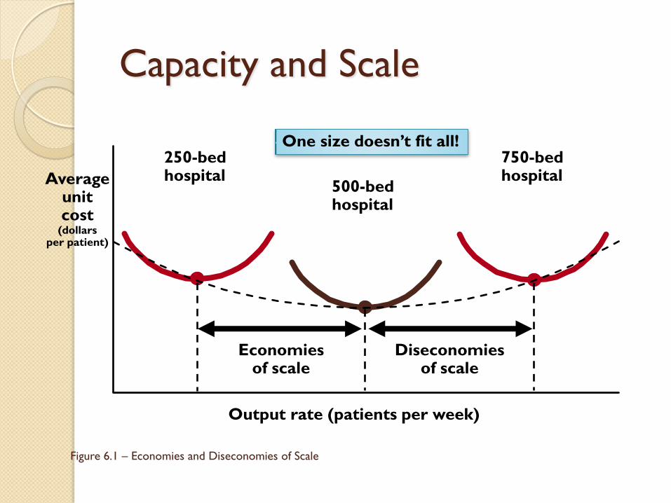
Capacity and Scale
Figure 6.1 – Economies and Diseconomies of Scale
250-bed hospital
500-bed hospital
750-bed hospital
Output rate (patients per week)
Average unit cost
(dollars per patient)
Economies of scale
Diseconomies of scale
One size doesn’t fit all!
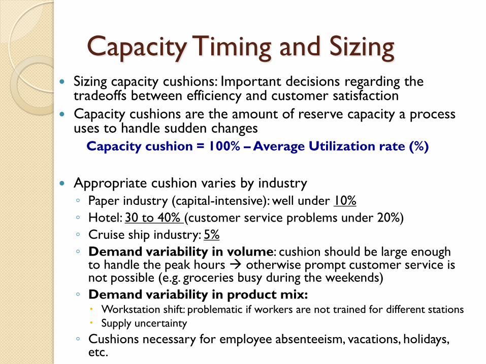
Capacity Timing and Sizing Sizing capacity cushions: Important decisions regarding the
tradeoffs between efficiency and customer satisfaction
Capacity cushions are the amount of reserve capacity a process uses to handle sudden changes
Appropriate cushion varies by industry
◦ Paper industry (capital-intensive): well under 10%
◦ Hotel: 30 to 40% (customer service problems under 20%)
◦ Cruise ship industry: 5%
◦ Demand variability in volume: cushion should be large enough to handle the peak hours otherwise prompt customer service is not possible (e.g. groceries busy during the weekends)
◦ Demand variability in product mix: Workstation shift: problematic if workers are not trained for different stations
Supply uncertainty
◦ Cushions necessary for employee absenteeism, vacations, holidays, etc.
Capacity cushion = 100% – Average Utilization rate (%)
Capacity Timing and Sizing
Decision related to when to adjust
capacity levels and by how much
◦ Expansionist strategy
◦ Wait-and-see strategy
◦ Combination strategy
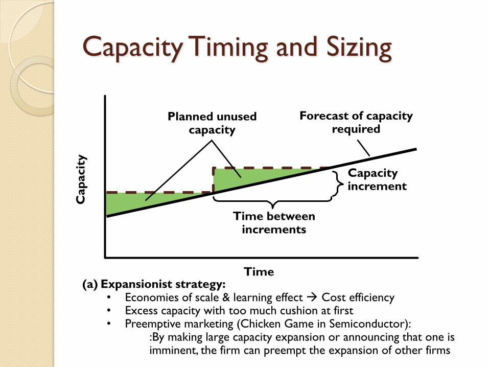
Capacity Timing and Sizing
Planned unused capacity
Time
Cap
acit
y
Forecast of capacity required
Time between increments
Capacity increment
(a) Expansionist strategy: • Economies of scale & learning effect Cost efficiency • Excess capacity with too much cushion at first • Preemptive marketing (Chicken Game in Semiconductor):
:By making large capacity expansion or announcing that one is imminent, the firm can preempt the expansion of other firms

Time
Cap
acit
y
(b) Wait-and-see strategy • Reduced risk of overexpansion • Possibility of preemption or incapability to meet the high demand surge
Planned use of short-term options
(overtime, temporary workers, subcontractors, etc.)
Time between increments
Capacity increment
Capacity Timing and Sizing
Forecast of capacity required
Linking Capacity
Capacity decisions should be linked to processes and supply chains throughout the organization
Important issues are competitive priorities, quality, and process design
◦ Higher level of capacity cushion Competitive priorities on fast delivery (competitive priorities)
Higher level of the service quality (quality)
Larger investment in capital intensive equipment or higher level of worker flexibility (process design)
Systematic Approach
1. Estimate future capacity requirements
2. Identify gaps by comparing requirements
with available capacity
3. Develop alternative plans for reducing the
gaps
4. Evaluate each alternative, both qualitatively
and quantitatively, and make a final choice
Systematic Approach
Step 1 is to determine the capacity required to meet future demand using an appropriate planning horizon
Capacity requirement: capacity required for some future time period to meet the demand
◦ Demand forecast, productivity, competition, and technological change in consideration
Output measures based on rates of production
Input measures may be used when
◦ Product variety and process divergence is high
◦ The product or service mix is changing
◦ Productivity rates are expected to change
◦ Significant learning effects are expected
◦ e.g. the number of employees, machines, trucks, etc.

Systematic Approach
For one service or product processed at one
operation with a one year time period, the
capacity requirement, M, is
Capacity requirement
= Processing hours required for year’s demand
Hours available from a single capacity unit (such as an employee or machine) per year,
after deducting desired cushion
M = Dp
N[1 – (C/100)]
where
D = demand forecast for the year (number of customers serviced or units of product)
p = processing time (in hours per customer served or unit produced)
N = total number of hours per year during which the process operates
C = desired capacity cushion (expressed as a percent)
Systematic Approach
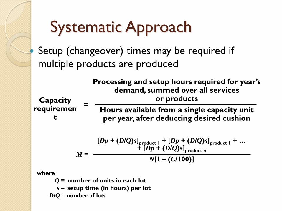
Setup (changeover) times may be required if
multiple products are produced
Capacity requiremen
t
=
Processing and setup hours required for year’s demand, summed over all services
or products
Hours available from a single capacity unit per year, after deducting desired cushion
M =
[Dp + (D/Q)s]product 1 + [Dp + (D/Q)s]product 1 + … + [Dp + (D/Q)s]product n
N[1 – (C/100)]
where
Q = number of units in each lot
s = setup time (in hours) per lot
D/Q = number of lots
Estimating Capacity Requirements
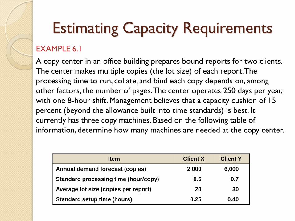
EXAMPLE 6.1
A copy center in an office building prepares bound reports for two clients.
The center makes multiple copies (the lot size) of each report. The
processing time to run, collate, and bind each copy depends on, among
other factors, the number of pages. The center operates 250 days per year,
with one 8-hour shift. Management believes that a capacity cushion of 15
percent (beyond the allowance built into time standards) is best. It
currently has three copy machines. Based on the following table of
information, determine how many machines are needed at the copy center.
Item Client X Client Y
Annual demand forecast (copies) 2,000 6,000
Standard processing time (hour/copy) 0.5 0.7
Average lot size (copies per report) 20 30
Standard setup time (hours) 0.25 0.40
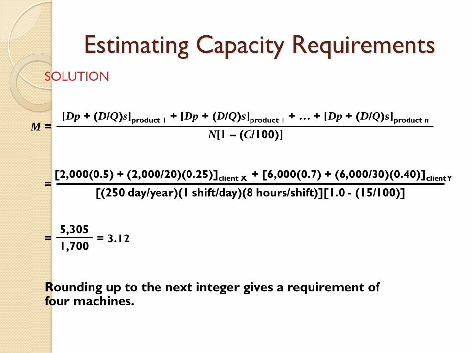
Estimating Capacity Requirements SOLUTION
M = [Dp + (D/Q)s]product 1 + [Dp + (D/Q)s]product 1 + … + [Dp + (D/Q)s]product n
N[1 – (C/100)]
= [2,000(0.5) + (2,000/20)(0.25)]client X + [6,000(0.7) + (6,000/30)(0.40)]client Y
[(250 day/year)(1 shift/day)(8 hours/shift)][1.0 - (15/100)]
= = 3.12 5,305
1,700
Rounding up to the next integer gives a requirement of four machines.
Systematic Approach
Step 2 is to identify gaps between projected capacity requirements (M) and current capacity
◦ Complicated by multiple operations and resource inputs
Step 3 is to develop alternatives
Base case is to do nothing and suffer the consequences
Many different alternatives are possible: base case, long-term expansion, short-term remedies
Systematic Approach
Step 4 is to evaluate the alternatives
◦ Qualitative concerns include strategic fit and
various uncertainty (demand, competition,
technological change, cost estimates)
◦ Quantitative concerns may include cash flows and
other quantitative measures
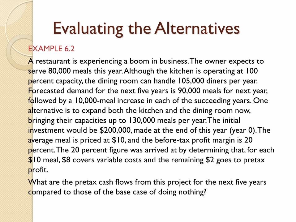
Evaluating the Alternatives EXAMPLE 6.2
A restaurant is experiencing a boom in business. The owner expects to
serve 80,000 meals this year. Although the kitchen is operating at 100
percent capacity, the dining room can handle 105,000 diners per year.
Forecasted demand for the next five years is 90,000 meals for next year,
followed by a 10,000-meal increase in each of the succeeding years. One
alternative is to expand both the kitchen and the dining room now,
bringing their capacities up to 130,000 meals per year. The initial
investment would be $200,000, made at the end of this year (year 0). The
average meal is priced at $10, and the before-tax profit margin is 20
percent. The 20 percent figure was arrived at by determining that, for each
$10 meal, $8 covers variable costs and the remaining $2 goes to pretax
profit.
What are the pretax cash flows from this project for the next five years
compared to those of the base case of doing nothing?

Evaluating the Alternatives SOLUTION
Recall that the base case of doing nothing results in losing all potential
sales beyond 80,000 meals. With the new capacity, the cash flow would
equal the extra meals served by having a 130,000-meal capacity, multiplied
by a profit of $2 per meal. In year 0, the only cash flow is –$200,000 for the
initial investment. In year 1, the 90,000-meal demand will be completely
satisfied by the expanded capacity, so the incremental cash flow is (90,000
– 80,000)($2) = $20,000. For subsequent years, the figures are as follows:
Year 2: Demand = 100,000; Cash flow = (100,000 – 80,000)$2 = $40,000
Year 3: Demand = 110,000; Cash flow = (110,000 – 80,000)$2 = $60,000
Year 4: Demand = 120,000; Cash flow = (120,000 – 80,000)$2 = $80,000
Year 5: Demand = 130,000; Cash flow = (130,000 – 80,000)$2 = $100,000

Evaluating the Alternatives
If the new capacity were smaller than the expected demand in any year, we
would subtract the base case capacity from the new capacity (rather than
the demand). The owner should account for the time value of money,
applying such techniques as the net present value or internal rate of return
methods. For instance, the net present value (NPV) of this project at a
discount rate of 10 percent is calculated here, and equals $13,051.76.
NPV = –200,000 + [(20,000/1.1)] + [40,000/(1.1)2] +
[60,000/(1.1)3] + [80,000/(1.1)4] + [100,000/(1.1)5]
= –$200,000 + $18,181.82 + $33,057.85 + $45,078.89 +
$54,641.07 + $62,092.13
= $13,051.76
Tools for Capacity Planning
Waiting-line models
◦ Useful in high customer-contact processes
Simulation
Can be used when models are too complex for waiting-line analysis
Decision trees
Useful when demand is uncertain and sequential decisions are involved

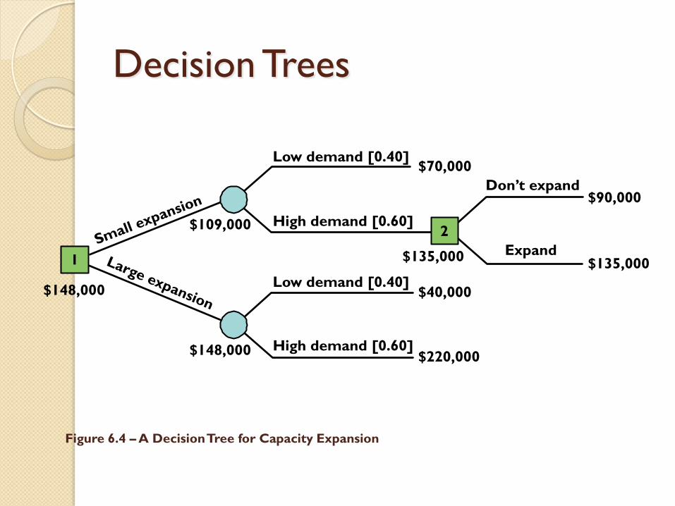
Decision Trees
1
Low demand [0.40]
High demand [0.60]
Low demand [0.40]
High demand [0.60]
$70,000
$220,000
$40,000
$135,000
$90,000 Don’t expand
Expand
2
Figure 6.4 – A Decision Tree for Capacity Expansion
$135,000
$109,000
$148,000
$148,000
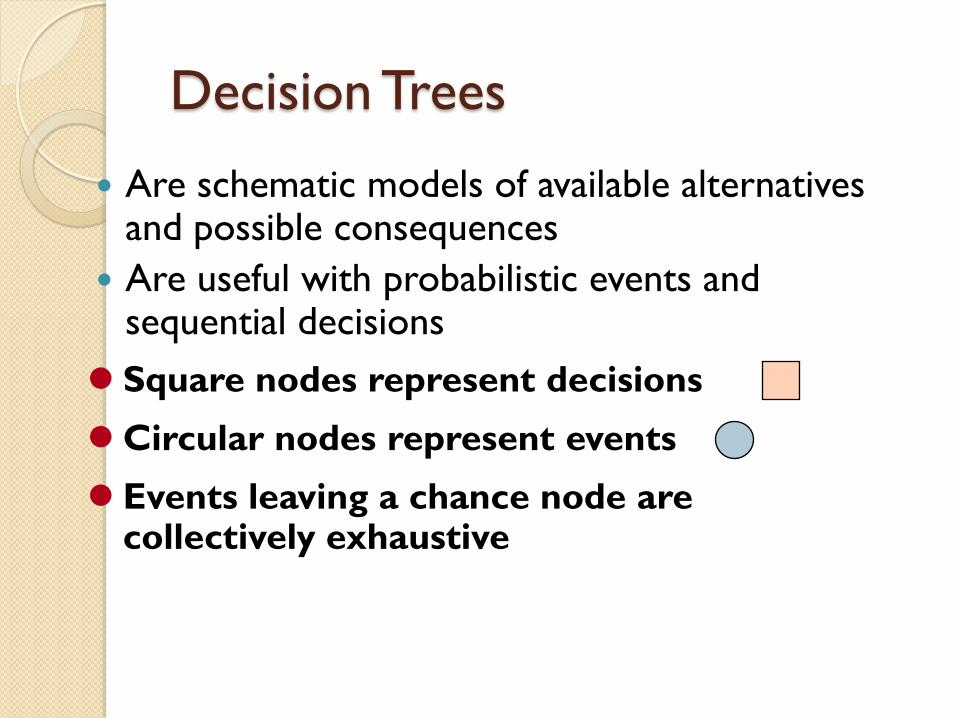
Are schematic models of available alternatives and possible consequences
Are useful with probabilistic events and sequential decisions
Decision Trees
Square nodes represent decisions
Circular nodes represent events
Events leaving a chance node are collectively exhaustive
Conditional payoffs for each possible alternative-event combination shown at the end of each combination
Draw the decision tree from left to right
Calculate expected payoff to solve the decision tree from right to left
Decision Trees

Payoff 1
Payoff 2
Payoff 3
Alternative 3
Alternative 4
Alternative 5
Payoff 1
Payoff 2
Payoff 3
E1 & Probability
E2 & Probability
E3 & Probability
E2 & Probability
E3 & Probability
Payoff 1
Payoff 2
1st decision
1
Possible 2nd decision
2
Decision Trees
= Event node
= Decision node
Ei = Event i
P(Ei) = Probability of event i FIGURE A.4 – A Decision Tree Model
Decision Trees
After drawing a decision tree, we solve it by
working from right to left, calculating the
expected payoff for each of its possible paths
1. For an event node, we multiply the payoff of each event branch by the event’s probability and add these products to get the event node’s expected payoff
2. For a decision node, we pick the alternative that has the best expected payoff
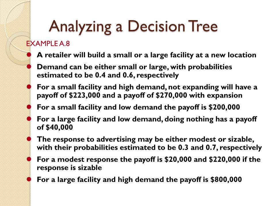
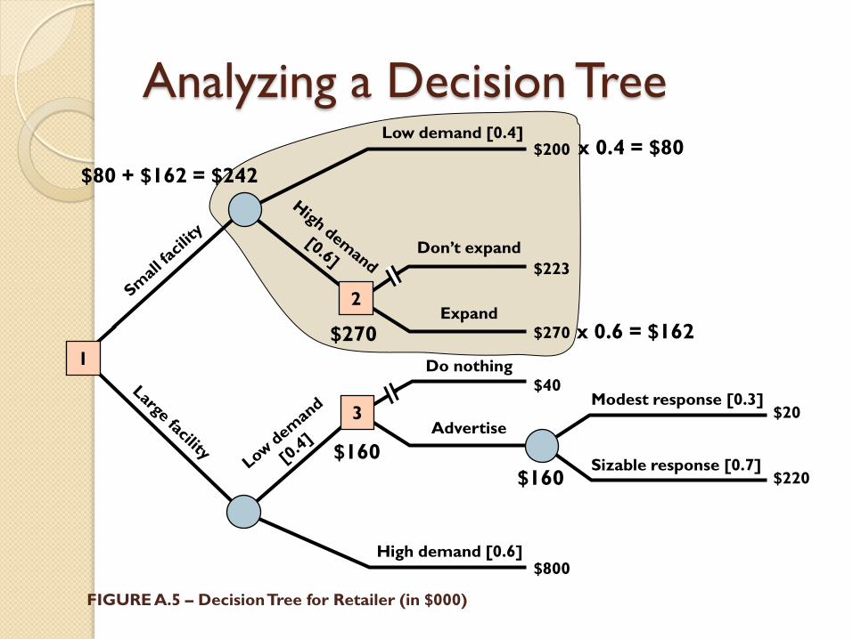
Analyzing a Decision Tree EXAMPLE A.8
A retailer will build a small or a large facility at a new location
Demand can be either small or large, with probabilities estimated to be 0.4 and 0.6, respectively
For a small facility and high demand, not expanding will have a payoff of $223,000 and a payoff of $270,000 with expansion
For a small facility and low demand the payoff is $200,000
For a large facility and low demand, doing nothing has a payoff of $40,000
The response to advertising may be either modest or sizable, with their probabilities estimated to be 0.3 and 0.7, respectively
For a modest response the payoff is $20,000 and $220,000 if the response is sizable
For a large facility and high demand the payoff is $800,000

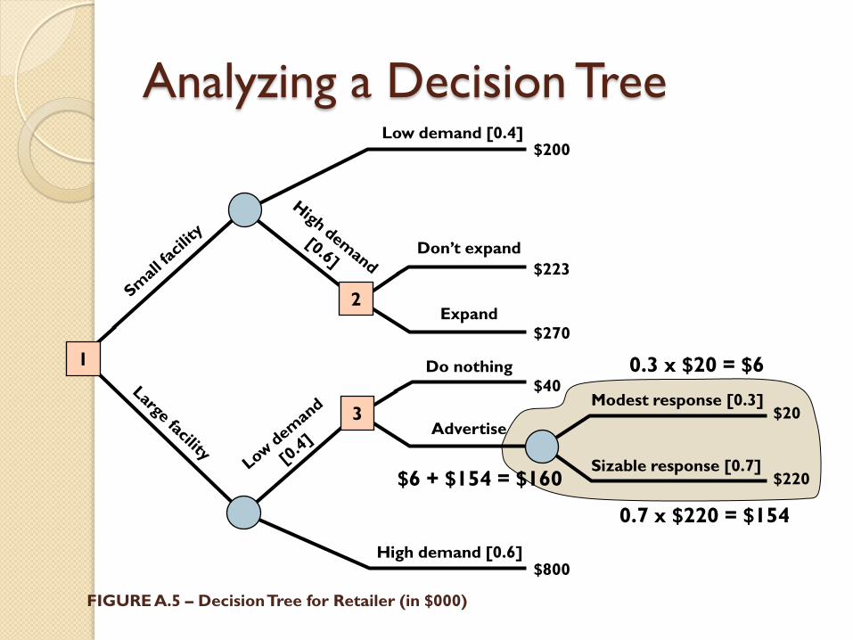
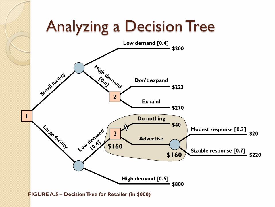
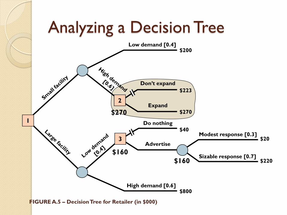
Analyzing a Decision Tree
SOLUTION
The decision tree in Figure A.5 shows the event probability and the payoff for each of the seven alternative-event combinations. The first decision is whether to build a small or a large facility. Its node is shown first, to the left, because it is the decision the retailer must make now. The second decision node is reached only if a small facility is built and demand turns out to be high. Finally, the third decision point is reached only if the retailer builds a large facility and demand turns out to be low.

Analyzing a Decision Tree $200
$223
$270
$40
$800
$20
$220
Don’t expand
Expand
Low demand [0.4]
2
FIGURE A.5 – Decision Tree for Retailer (in $000)
High demand [0.6]
3
Do nothing
Advertise
Modest response [0.3]
Sizable response [0.7]
1
Analyzing a Decision Tree $200
$223
$270
$40
$800
$20
$220
Don’t expand
Expand
Low demand [0.4]
2
FIGURE A.5 – Decision Tree for Retailer (in $000)
High demand [0.6]
3
Do nothing
Advertise
Modest response [0.3]
Sizable response [0.7]
1 0.3 x $20 = $6
0.7 x $220 = $154
$6 + $154 = $160
Analyzing a Decision Tree $200
$223
$270
$40
$800
$20
$220
Don’t expand
Expand
Low demand [0.4]
2
FIGURE A.5 – Decision Tree for Retailer (in $000)
High demand [0.6]
3
Do nothing
Advertise
Modest response [0.3]
Sizable response [0.7]
1
$160
$160
Analyzing a Decision Tree $200
$223
$270
$40
$800
$20
$220
Don’t expand
Expand
Low demand [0.4]
2
FIGURE A.5 – Decision Tree for Retailer (in $000)
High demand [0.6]
3
Do nothing
Advertise
Modest response [0.3]
Sizable response [0.7]
1
$160
$160
$270
Analyzing a Decision Tree $200
$223
$270
$40
$800
$20
$220
Don’t expand
Expand
Low demand [0.4]
2
FIGURE A.5 – Decision Tree for Retailer (in $000)
High demand [0.6]
3
Do nothing
Advertise
Modest response [0.3]
Sizable response [0.7]
1
$160
$160
$270
x 0.4 = $80
x 0.6 = $162
$80 + $162 = $242
Analyzing a Decision Tree $200
$223
$270
$40
$800
$20
$220
Don’t expand
Expand
Low demand [0.4]
2
FIGURE A.5 – Decision Tree for Retailer (in $000)
High demand [0.6]
3
Do nothing
Advertise
Modest response [0.3]
Sizable response [0.7]
1
$160
$160
$270
$242
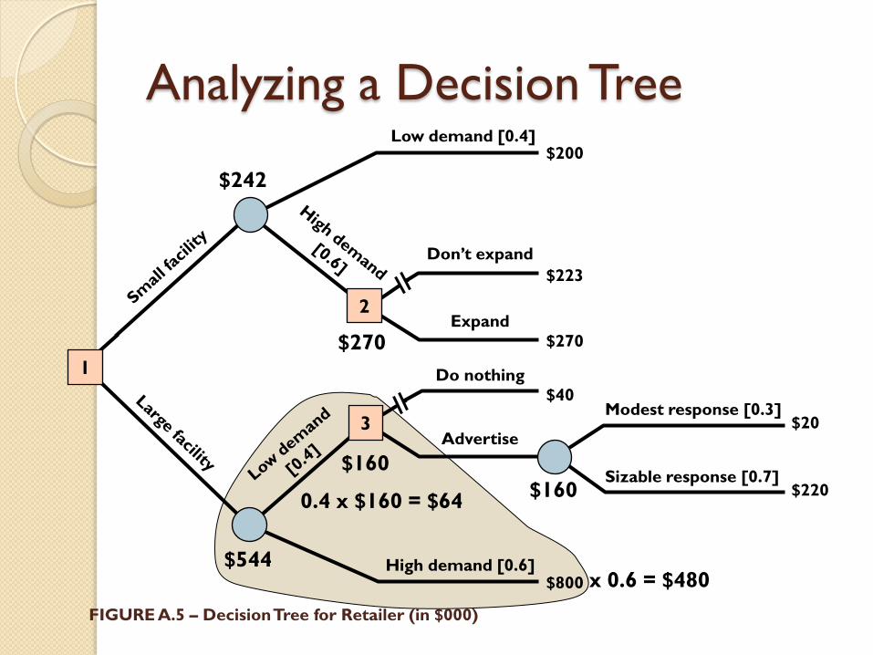
x 0.6 = $480
0.4 x $160 = $64
$544

Analyzing a Decision Tree $200
$223
$270
$40
$800
$20
$220
Don’t expand
Expand
Low demand [0.4]
2
FIGURE A.5 – Decision Tree for Retailer (in $000)
High demand [0.6]
3
Do nothing
Advertise
Modest response [0.3]
Sizable response [0.7]
1
$160
$160
$270
$242
$544
$544

Analyzing a Decision Tree $200
$223
$270
$40
$800
$20
$220
Don’t expand
Expand
Low demand [0.4]
2
FIGURE A.5 – Decision Tree for Retailer (in $000)
High demand [0.6]
3
Do nothing
Advertise
Modest response [0.3]
Sizable response [0.7]
1
$160
$160
$270
$242
$544
$544

Application A.6
Fletcher (a realist), Cooper (a pessimist), and Wainwright (an optimist) are joint owners in a company. They must decide whether to make Arrows, Barrels, or Wagons. The government is about to issue a policy and recommendation on pioneer travel that depends on whether certain treaties are obtained. The policy is expected to affect demand for the products; however it is impossible at this time to assess the probability of these policy “events.” The following data are available:
a. Draw the decision tree for the Fletcher, Cooper, and Wainwright using the following table
b. What is the expected payoff for the best alternative in the decision tree below?
Alternative
Land routes,
No Treaty
(0.50)
Land Routes,
Treaty Only
(0.30)
Sea routes,
Only (0.20)
Arrows 840,000 440,000 190,000
Barrels 370,000 220,000 670,000
Wagons 25,000 1,150,000 -25,000

Application A.6
Decision Trees
1
Low demand [0.40]
High demand [0.60]
Low demand [0.40]
High demand [0.60]
$70,000
$220,000
$40,000
$135,000
$90,000 Don’t expand
Expand
2
Figure 6.4 – A Decision Tree for Capacity Expansion
$135,000
$109,000
$148,000
$148,000
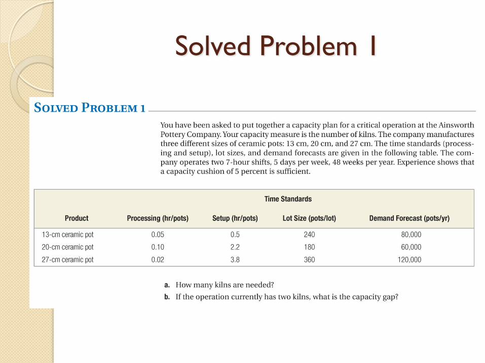
Solved Problem 1

Solved Problem 1
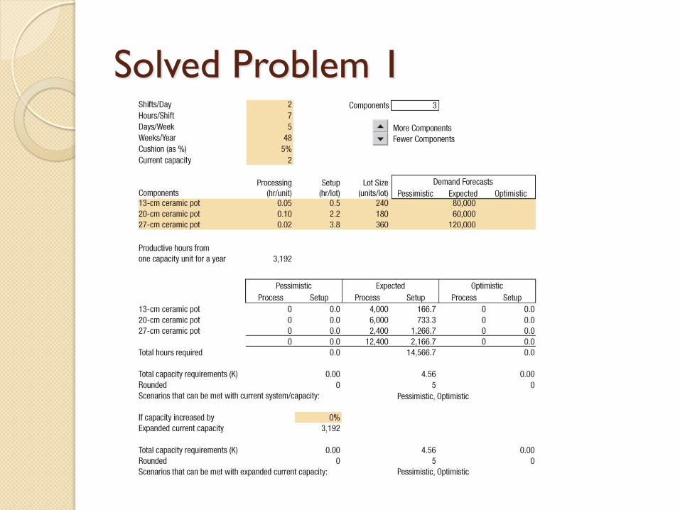
Solved Problem 1
Solved Problem 2
SOLUTION
Table 6.1 shows the cash inflows and outflows. The year 3 cash flow is
unusual in two respects. First, the cash inflow from sales is $50,000
rather than $60,000. The increase in sales over the base is 25,000
meals (105,000 – 10,000) instead of 30,000 meals (110,000 – 80,000)
because the restaurant’s capacity falls somewhat short of demand.
Second, a cash outflow of $170,000 occurs at the end of year 3, when
the second-stage expansion occurs.
The net cash flow for year 3 is $50,000 – $170,000 = –$120,000.

Solved Problem 2
The base case for Grandmother’s Chicken Restaurant (see Example 6.2) is
to do nothing. The capacity of the kitchen in the base case is 80,000 meals
per year. A capacity alternative for Grandmother’s Chicken Restaurant is a
two-stage expansion. This alternative expands the kitchen at the end of
year 0, raising its capacity from 80,000 meals per year to that of the dining
area (105,000 meals per year). If sales in year 1 and 2 live up to
expectations, the capacities of both the kitchen and the dining room will be
expanded at the end of year 3 to 130,000 meals per year. This upgraded
capacity level should suffice up through year 5. The initial investment would
be $80,000 at the end of year 0 and an additional investment of $170,000
at the end of year 3. The pretax profit is $2 per meal. What are the pretax
cash flows for this alternative through year 5, compared with the base
case?
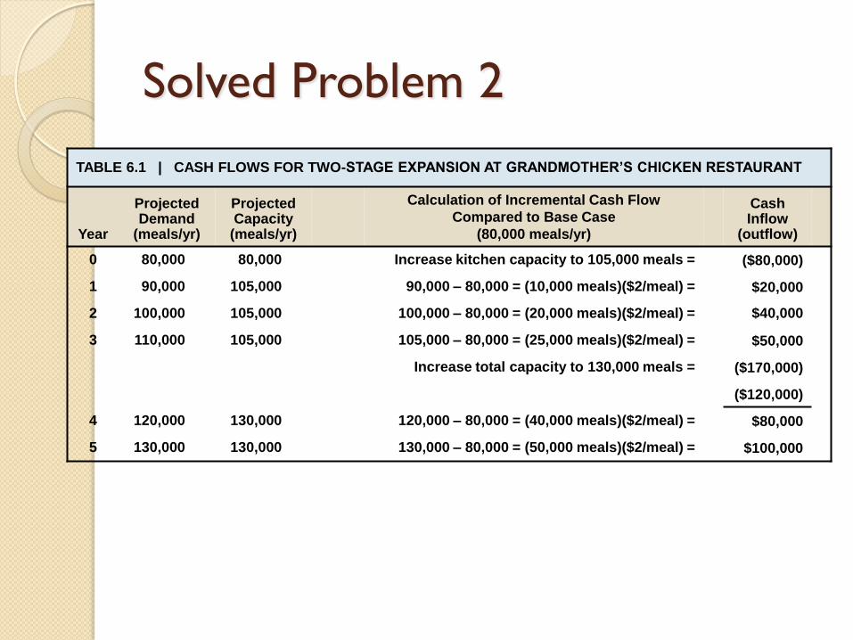
Solved Problem 2
TABLE 6.1 | CASH FLOWS FOR TWO-STAGE EXPANSION AT GRANDMOTHER’S CHICKEN RESTAURANT
Year
Projected Demand
(meals/yr)
Projected Capacity
(meals/yr)
Calculation of Incremental Cash Flow
Compared to Base Case
(80,000 meals/yr)
Cash Inflow
(outflow)
0 80,000 80,000 Increase kitchen capacity to 105,000 meals = ($80,000)
1 90,000 105,000 90,000 – 80,000 = (10,000 meals)($2/meal) = $20,000
2 100,000 105,000 100,000 – 80,000 = (20,000 meals)($2/meal) = $40,000
3 110,000 105,000 105,000 – 80,000 = (25,000 meals)($2/meal) = $50,000
Increase total capacity to 130,000 meals = ($170,000)
($120,000)
4 120,000 130,000 120,000 – 80,000 = (40,000 meals)($2/meal) = $80,000
5 130,000 130,000 130,000 – 80,000 = (50,000 meals)($2/meal) = $100,000

Solved Problem 2
NPV = –80,000 + (20,000/1.1) + [40,000/(1.1)2] – [120,000/(1.1)3] +
[80,000/(1.1)4] + [100,000/(1.1)5]
= –$80,000 + $18,181.82 + $33,057.85 – $90,157.77 + $54,641.07
+ $62,092.13
= –$2,184.90
For comparison purposes, the NPV of this project at a discount rate of 10 percent is calculated as follows, and equals negative $2,184.90.
On a purely monetary basis, a single-stage expansion seems to be a better alternative than this two-stage expansion. However, other qualitative factors as mentioned earlier must be considered as well.

End of Process Quality Session