This is an electronic reprint of the original article.This reprint may differ from the original in pagination and typographic detail.

Powered by TCPDF (www.tcpdf.org)

This material is protected by copyright and other intellectual property rights, and duplication or sale of all or part of any of the repository collections is not permitted, except that material may be duplicated by you for your research use or educational purposes in electronic or print form. You must obtain permission for any other use. Electronic or print copies may not be offered, whether for sale or otherwise to anyone who is not an authorised user.

Karvonen, Toni; Särkkä, SimoGaussian kernel quadrature at scaled Gauss–Hermite nodes

Published in:BIT - Numerical Mathematics

DOI:10.1007/s10543-019-00758-3

Published: 01/01/2019

Document VersionPublisher's PDF, also known as Version of record

Please cite the original version:Karvonen, T., & Särkkä, S. (2019). Gaussian kernel quadrature at scaled Gauss–Hermite nodes. BIT -Numerical Mathematics, 877–902. https://doi.org/10.1007/s10543-019-00758-3

BIT Numerical Mathematicshttps://doi.org/10.1007/s10543-019-00758-3

Gaussian kernel quadrature at scaled Gauss–Hermite nodes

Toni Karvonen1 · Simo Särkkä1

Received: 3 May 2018 / Accepted: 5 June 2019© The Author(s) 2019

AbstractThis article derives an accurate, explicit, and numerically stable approximation to thekernel quadrature weights in one dimension and on tensor product grids when thekernel and integration measure are Gaussian. The approximation is based on use ofscaled Gauss–Hermite nodes and truncation of the Mercer eigendecomposition of theGaussian kernel. Numerical evidence indicates that both the kernel quadrature and theapproximate weights at these nodes are positive. An exponential rate of convergencefor functions in the reproducing kernel Hilbert space induced by the Gaussian kernel isprovedunder an assumption ongrowth of the sumof absolute values of the approximateweights.

Keywords Numerical integration · Kernel quadrature · Gaussian quadrature · Mercereigendecomposition

Mathematics Subject Classification 45C05 · 46E22 · 47B32 · 65D30 · 65D32

1 Introduction

Let μ be the standard Gaussian measure on R and f : R → R a measurable function.We consider the problem of numerical computation of the integral with respect to μ

of f using a kernel quadrature rule (we reserve the term cubature for rules on higher

Communicated by Tom Lyche.

This work was supported by the Aalto ELEC Doctoral School as well as Academy of Finland projects266940, 304087, and 313708.

B Toni Karvonentoni.karvonen@aalto.fi

Simo Särkkäsimo.sarkka@aalto.fi

1 Department of Electrical Engineering and Automation, Aalto University, Espoo, Finland

123

T. Karvonen, S. Särkkä

dimensions) based on the Gaussian kernel

k(x, y) = exp

(− (x − y)2

2�2

)(1.1)

with the length-scale � > 0.Given any distinct nodes x1, . . . , xN , the kernel quadraturerule is an approximation of the form

Qk( f ) :=N∑

n=1

wk,n f (xn) ≈ μ( f ) := 1√2π

∫R

f (x) e−x2/2 dx,

with its weights wk = (wk,1, . . . , wk,N )∈RN solved from the linear system of equa-tions

Kwk = kμ, (1.2)

where [K ]i j := k(xi , x j ) and [kμ]i := ∫R

k(xi , x)dμ(x). This is equivalent to uniquelyselecting the weights such that the N kernel translates k(x1, ·), . . . , k(xN , ·) are inte-grated exactly by the quadrature rule. Kernel quadrature rules can be interpreted as bestquadrature rules in the reproducing kernelHilbert space (RKHS) induced by a positive-definite kernel [20], integrated kernel (radial basis function) interpolants [5,35], andposteriors to μ( f ) under a Gaussian process prior on the integrand [7,21,29].

Recently, Fasshauer and McCourt [12] have developed a method to circumventthe well-known problem that interpolation with the Gaussian kernel becomes oftennumerically unstable—in particular when � is large—because the condition numberof K tends to grow with an exponential rate [33]. They do this by truncating theMercer eigendecomposition of the Gaussian kernel after M terms and replacing theinterpolation basis {k(xn, ·)}N

n=1 with the first M eigenfunctions. In this article weshow that application of this method with M = N to kernel quadrature yields, whenthe nodes are selected by a suitable and fairly natural scaling of the nodes of theclassical Gauss–Hermite quadrature rule, an accurate, explicit, and numerically stableapproximation to the Gaussian kernel quadrature weights. Moreover, the proposednodes appear to be a good and natural choice for the Gaussian kernel quadrature.

To be precise, Theorem 2.2 states that the quadrature rule Qk that exactly integratesthe first N Mercer eigenfunctions of the Gaussian kernel and uses the nodes

xn := 1√2αβ

xGHn

has the weights

wk,n :=(

1

1 + 2δ2

)1/2wGH

n eδ2 x2n

�(N−1)/2�∑m=0

1

2mm!(2α2β2

1 + 2δ2− 1

)m

H2m(xGHn ),

123

Gaussian kernel quadrature at scaled Gauss–Hermite nodes

wk = (wk,1, . . . , wk,N )∈RN , where α (for which the value 1/

√2 seems the most

natural), β, and δ are constants defined in Eq. (2.3), Hn are the probabilists’ Hermitepolynomials (2.2), and xGH

n and wGHn are the nodes and weights of the N -point Gauss–

Hermite quadrature rule. We argue that these weights are a good approximation to wk

and accordingly call them approximate Gaussian kernel quadrature weights. Althoughwe derive no bounds for the error of this weight approximation, numerical experimentsin Sect. 5 indicate that the approximation is accurate and that it appears that wk → wk

as N → ∞. In Sect. 4we extend theweight approximation ford-dimensionalGaussiantensor product kernel cubature rules of the form

Qdk = Qk,1 ⊗ · · · ⊗ Qk,d ,

where Qk,i are one-dimensional Gaussian kernel quadrature rules. Since each weightof Qd

k is a product of weights of the univariate rules, an approximation for the tensorproduct weights is readily available.

It turns out that the approximate weight and the associated nodes xn have a numberof desirable properties:

– We are not aware of any work on efficient selection of “good” nodes in the settingof this article. The Gauss–Hermite nodes [29, Section 3] and random points [31]are often used, but one should clearly be able to do better, while computation ofthe optimal nodes [28, Section 5.2] is computationally demanding. As such, giventhe desirable properties, listed below, of the resulting kernel quadrature rules, thenodes xn appear to be an excellent heuristic choice. These nodes also behavenaturally when � → ∞; see Sect. 2.5.

– Numerical experiments in Sect. 5.3 suggest that both wk,n (for the nodes xn) andwk,n are positive for any N ∈ N and every n = 1, . . . , N . Besides the optimalnodes, the weights for which are guaranteed to be positive when the Gaussiankernel is used [28,32], there are no node configurations that give rise to positiveweights as far as we are aware of.

– Numerical experiments in Sects. 5.1 and 5.3 demonstrate that computation of theapproximate weights is numerically stable. Furthermore, construction of theseweights only incurs a quadratic computational cost in the number of points, asopposed to the cubic cost of solving wk from Eq. (1.2). See Sect. 2.6 for moredetails. Note that to obtain a numerically stable method it is not necessary to usethe nodes xn as the method in [12] can be applied in a straightforward manner forany nodes. However, doing so one forgoes a closed form expression and has to usethe QR decomposition.

– In Sects. 3 and 4we show that slow enough growthwith N of∑N

n=1

∣∣wk,n∣∣ (numer-

ical evidence indicates this sum converges to one) guarantees that the approximateGaussian kernel quadrature rule—as well as the corresponding tensor productversion—converges with an exponential rate for functions in the RKHS of theGaussian kernel. Convergence analysis is based on analysis of magnitude of theremainder of the Mercer expansion and rather explicit bounds on Hermite poly-nomials and their roots. Magnitude of the nodes xn is crucial for the analysis; ifthey were further spread out the proofs would not work as such.

123

T. Karvonen, S. Särkkä

– We find the connection to the Gauss–Hermite weights and nodes that the closedform expression for wk provides intriguing and hope that it can be at some pointused to furnish, for example, a rigorous proof of positivity of the approximateweights.

2 Approximate weights

This section contains the main results of this article. The main contribution is deriva-tion, in Theorem 2.2, of the weights wk , that can be used to approximate the kernelquadrature weights. We also discuss positivity of these weights, the effect the kernellength-scale � is expected to have on quality of the approximation, and computationalcomplexity.

2.1 Eigendecomposition of the Gaussian kernel

Let ν be a probability measure on the real line. If the support of ν is compact, Mer-cer’s theorem guarantees that any positive-definite kernel k admits an absolutely anduniformly convergent eigendecomposition

k(x, y) =∞∑

n=0

λnϕn(x)ϕn(y) (2.1)

for positive and non-increasing eigenvalues λn and eigenfunctions ϕn that are includedin the RKHS H induced by k and orthonormal in L2(ν). Moreover,

√λnϕn are

H -orthonormal. If the support of ν is not compact, the expansion (2.1) con-verges absolutely and uniformly on all compact subsets of R × R under some mildassumptions [37,38]. For the Gaussian kernel (1.1) and measure the eigenvalues andeigenfunctions are available analytically. For a collection of explicit eigendecompo-sitions of some other kernels, see for instance [11, Appendix A]

Let μα stand for the Gaussian probability measure,

dμα(x) := α√πe−α2x2 dx,

with variance 1/(2α2) (i.e., μ = μ1/√2 ) and

Hn(x) := (−1)n ex2/2 dn

dxne−x2/2 (2.2)

for the (unnormalised) probabilists’ Hermite polynomial satisfying the orthogonalityproperty 〈Hn,Hm〉L2(μ) = n! δnm . Denote

ε = 1√2�

, β =(1 +(2ε

α

)2)1/4, and δ2 = α2

2(β2 − 1) (2.3)

123

Gaussian kernel quadrature at scaled Gauss–Hermite nodes

and note that β > 1 and δ2 > 0. Then the eigenvalues and L2(μα)-orthonormaleigenfunctions of the Gaussian kernel are [12]

λαn :=√

α2

α2 + δ2 + ε2

(ε2

α2 + δ2 + ε2

)n

(2.4)

and

ϕαn (x) :=

√β

n! e−δ2x2 Hn

(√2αβx

). (2.5)

See [11, Section 12.2.1] for verification that these indeed are Mercer eigenfunctionsand eigenvalues for the Gaussian kernel. The role of the parameter α is discussed inSect. 2.4. The following result, also derivable from Equation 22.13.17 in [1], will beuseful.

Lemma 2.1 The eigenfunctions (2.5) of the Gaussian kernel (1.1) satisfy

μ(ϕα2m+1) = 0 and μ(ϕα

2m) =(

β

1 + 2δ2

)1/2√(2m)!2mm!

(2α2β2

1 + 2δ2− 1

)m

for m ≥ 0.

Proof Since an Hermite polynomial of odd order is an odd function, μ(ϕα2m+1) = 0.

For even indices, use the explicit expression

H2m(x) = (2m)!2m

m∑p=0

(−1)m−p

(2p)!(m − p)!(√

2x)2p

,

the Gaussian moment formula∫R

x2p e−δ2x2 dμ(x) = 1√2π

∫R

x2p e−(δ2+1/2)x2 dx = (2p)!2p p!(1 + 2δ2)p+1/2 ,

and the binomial theorem to conclude that

μ(ϕα2m) =

√(2m)!β2m

m∑p=0

(−1)m−p

(2p)!(m − p)! (2αβ)2p∫R

x2p e−δ2x2 dμ(x)

= (−1)m√(2m)!β

2m√1 + 2δ2

m∑p=0

1

p!(m − p)!(

− 2α2β2

1 + 2δ2

)p

= (−1)m√(2m)!β

2mm!√1 + 2δ2

m∑p=0

(m

p

)(− 2α2β2

1 + 2δ2

)p

=(

β

1 + 2δ2

)1/2 √(2m)!2mm!

(2α2β2

1 + 2δ2− 1

)m

.

�

123

T. Karvonen, S. Särkkä

2.2 Approximation via QR decomposition

We begin by outlining a straightforward extension to kernel quadrature of the workof Fasshauer and McCourt in [12] and [11, Chapter 13] on numerically stable kernelinterpolation. Recall that the kernel quadrature weights wk ∈ R

N at distinct nodesx1, . . . , xN are solved from the linear system Kwk = kμ with [K ]i j = k(xi , x j )

and [kμ]i = ∫R

k(xi , x)dμ(x). Truncation of the eigendecomposition (2.1) afterM ≥ N terms1 yields the approximations K ≈ ΦΛΦT and kμ ≈ ΦΛϕμ, where[Φ]i j := ϕα

j−1(xi ) is an N × M matrix, the diagonal M × M matrix [Λ]i i := λi−1contains the eigenvalues in appropriate order, and [ϕμ]i := μ(ϕi−1) is an M-vector.The kernel quadrature weights wk can be therefore approximated by

wMk := (ΦΛΦT)−1

ΦΛϕμ. (2.6)

Equation (2.6) can be written in a more convenient form by exploiting the QRdecomposition. The QR decomposition of Φ is

Φ = Q R := Q[

R1 R2

]

for a unitary Q ∈ RN×N , an upper triangular R1 ∈ R

N×N , and R2 ∈ RN×(M−N ).

Consequently,

wMk = (Q RΛRTQT)−1

Q RΛϕμ = Q(RΛRT)−1

RΛϕμ.

The decomposition

Λ =[Λ1 00 Λ2

]

of Λ ∈ RM×M into diagonal Λ1 ∈ R

N×N and Λ2 ∈ R(M−N )×(M−N ) allows for

writing

RΛRT = R1Λ1(RT1 + Λ−1

1 R−11 R2Λ2RT

2

).

Therefore,

wMk = Q

(RT1 + Λ−1

1 R−11 R2Λ2RT

2

)−1[

IN Λ−11 R−1

1 R2Λ2

]ϕμ, (2.7)

where IN is the N × N identity matrix. If ε2/(α2 + δ2 + ε2) is small (i.e., � islarge), numerical ill-conditioning in Eq. (2.7) for the Gaussian kernel is associatedwith the diagonal matrices Λ−1

1 and Λ2. Consequently, numerical stability can besignificantly improved by performing the multiplications by these matrices in the

1 Low-rank approximations (i.e., M < N ) are also possible [12, Section 6.1].

123

Gaussian kernel quadrature at scaled Gauss–Hermite nodes

terms Λ−11 R−1

1 R2Λ2RT2 and Λ−1

1 R−11 R2Λ2 analytically; see [12, Sections 4.1 and

4.2] for more details.Unfortunately, using the QR decomposition does not provide an attractive closed

form solution for the approximate weights wMk for general M . Setting M = N turns

Φ into a square matrix, enabling its direct inversion and formation of an explicit con-nection to the classical Gauss–Hermite quadrature. The rest of the article is concernedwith this special case.

2.3 Gauss–Hermite quadrature

Given a measure ν onR, the N -point Gaussian quadrature rule is the unique N -pointquadrature rule that is exact for all polynomials of degree at most 2N − 1. We areinterested in Gauss–Hermite quadrature rules that are Gaussian rules for the Gaussianmeasure μ:

N∑n=1

wGHn p(xGH

n ) = μ(p)

for every polynomial p : R → R with deg p ≤ 2N − 1. The nodes xGH1 , . . . xGH

Nare the roots of the N th Hermite polynomial HN and the weights wGH

1 , . . . , wGHN are

positive and sum to one. The nodes and the weights are related to the eigenvaluesand eigenvectors of the tridiagonal Jacobi matrix formed out of three-term recurrencerelation coefficients of normalised Hermite polynomials [13, Theorem 3.1].

We make use of the following theorem, a one-dimensional special case of a moregeneral result due to Mysovskikh [27]. See also [8, Section 7]. This result also followsfrom the Christoffel–Darboux formula (2.12).

Theorem 2.1 Let ν be a measure on R. Suppose that x1, . . . , xN and w1, . . . , wN arethe nodes and weights of the unique Gaussian quadrature rule. Let p0, . . . , pN−1 bethe L2(ν)-orthonormal polynomials. Then the matrix [P]i j := ∑N−1

n=0 pn(xi )pn(x j )

is diagonal and has the diagonal elements [P]i i = 1/wi .

2.4 Approximate weights at scaled Gauss–Hermite nodes

Let us now consider the approximate weights (2.6) with M = N . Assuming that Φ isinvertible, we then have

wk ≈ wk := wNk = (ΦΛΦT)−1

ΦΛϕμ = Φ−Tϕμ.

Note that the exponentially decayingMercer eigenvalues, a major source of numericalinstability, do not appear in the equation for wk . The weights wk are those of theunique quadrature rule that is exact for the N first eigenfunctions ϕα

0 , . . . , ϕαN−1. For

the Gaussian kernel, we are in a position to do much more. Recalling the form ofthe eigenfunctions in Eq. (2.5), we can write Φ = √

βE−1V for the diagonal matrix

123

T. Karvonen, S. Särkkä

[E]i i := eδ2x2i and the Vandermonde matrix

[V ]i j := 1√( j − 1)!H j−1

(√2αβxi

)(2.8)

of scaled and normalised Hermite polynomials. From this it is evident that Φ isinvertible—which is just a manifestation of the fact that the eigenfunctions of a totallypositive kernel constitute a Chebyshev system [17,30]. Consequently,

wk = 1√β

EV −Tϕμ.

Select the nodes

xn := 1√2αβ

xGHn .

Then the matrix V defined in Eq. (2.8) is precisely the Vandermonde matrix of thenormalised Hermite polynomials and V V T is the matrix P of Theorem 2.1. Let WGH

be the diagonal matrix containing the Gauss–Hermite weights. It follows that V −T =WGHV and

wk = 1√β

EV −Tϕμ = 1√β

EWGHV ϕμ. (2.9)

Combining this equation with Lemma 2.1, we obtain the main result of this article.

Theorem 2.2 Let xGH1 , . . . , xGH

N and wGH1 , . . . , wGH

N stand for the nodes and weights ofthe N-point Gauss–Hermite quadrature rule. Define the nodes

xn = 1√2αβ

xGHn . (2.10)

Then the weights wk ∈ RN of the N-point quadrature rule

Qk( f ) :=N∑

n=1

wk,n f (xn),

defined by the exactness conditions Qk(ϕαn ) = μα(ϕα

n ) for n = 0, . . . , N − 1, are

wk,n =(

1

1 + 2δ2

)1/2wGH

n eδ2 x2n

�(N−1)/2�∑m=0

1

2mm!(2α2β2

1 + 2δ2− 1

)m

H2m(xGHn ),

(2.11)

where α, β, and δ are defined in Eq. (2.3) and H2m are the probabilists’ Hermitepolynomials (2.2).

123

Gaussian kernel quadrature at scaled Gauss–Hermite nodes

Since theweights wk are obtained by truncating of theMercer expansion of k, it is tobe expected that wk ≈ wk . Thismotivates our calling of theseweights the approximateGaussian kernel quadrature weights. We do not provide theoretical results on qualityof this approximation, but the numerical experiments in Sect. 5.2 indicate that theapproximation is accurate and that its accuracy increases with N . See [12] for relatedexperiments.

An alternative non-analytical formula for the approximate weights can be derivedusing the Christoffel–Darboux formula [13, Section 1.3.3]

M∑m=0

Hm(x)Hm(y)

m! = HM (y)HM+1(x) − HM (x)HM+1(y)

M !(x − y). (2.12)

From Eq. (2.9) we then obtain (keep in mind that xGH1 , . . . , xGH

N are the roots of HN )

wk,n = 1√β

wGHn eδ2 x2n

N−1∑m=0

1√m!Hm(xGH

n )μ(ϕαm)

= wGHn eδ2 x2n

∫R

e−δ2x2N−1∑m=0

Hm(xGHn )Hm(

√2αβx)

m! dμ(x)

= wGHn eδ2 x2n HN−1(xGH

n )√2π(N − 1)!

∫R

HN (√2αβx)√

2αβx − xGHn

e−(δ2+1/2)x2 dx

= wGHn eδ2 x2n HN−1(xGH

n )

2√

παβ(N − 1)!∫R

HN (x)

x − xGHn

exp

(− δ2 + 1/2

2α2β2 x2)dx .

This formula is analogous to the formula

wGHn = 1√

2π NHN−1(xGHn )

∫R

HN (x)

x − xGHn

e−x2/2 dx

for the Gauss–Hermite weights. Plugging this in, we get

wk,n = eδ2 x2n

2√2παβN !

∫R

HN (x)

x − xGHn

e−x2/2 dx∫R

HN (x)

x − xGHn

exp

(− δ2 + 1/2

2α2β2 x2)dx .

It appears that both wk,n and wk,n of Theorem 2.2 are positive for many choicesof α; see Sect. 5.3 for experiments involving α = 1/

√2. Unfortunately, we have

not been able to prove this. In fact, numerical evidence indicates something slightlystronger. Namely that the even polynomial

Rγ,N (x) :=�(N−1)/2�∑

m=0

γ m

2mm!H2m(x)

123

T. Karvonen, S. Särkkä

of degree 2�(N − 1)/2� is positive for every N ≥ 1 and (at least) every 0 < γ ≤ 1.This would imply positivity of wk,n since the Gauss–Hermite weightswGH

n are positive.For example, with α = 1/

√2,

2α2β2

1 + 2δ2− 1 = 2

√1 + 8ε2

1 + √1 + 8ε2

− 1 =√1 + 8ε2 − 1

1 + √1 + 8ε2

∈ (0, 1).

As discussed in [12] in the context of kernel interpolation, the parameter α actsas a global scale parameter. While in interpolation it is not entirely clear how thisparameter should be selected, in quadrature it seems natural to set α = 1/

√2 so that

the eigenfunctions are orthonormal in L2(μ). This is the value that we use, thoughalso other values are potentially of interest since α can be used to control the spreadof the nodes independently of the length-scale �. In Sect. 3, we also see that this valueleads to more natural convergence analysis.

2.5 Effect of the length-scale

Roughly speaking, magnitude of the eigenvalues

λαn =√

α2

α2 + δ2 + ε2

(ε2

α2 + δ2 + ε2

)n

determines how many eigenfunctions are necessary for an accurate weight approxi-mation. We therefore expect that the approximation (2.11) is less accurate when thelength-scale � is small (i.e., ε = 1/(

√2�) is large). This is confirmed by the numerical

experiments in Sect. 5.Consider then the case � → ∞. This scenario is called the flat limit in scattered

data approximation literature where it has been proved2 that the kernel interpolantassociated to an isotropic kernel with increasing length-scale converges to (i) theunique polynomial interpolant of degree N − 1 to the data if the kernel is infinitelysmooth [22,24,34] or (ii) to a polyharmonic spline interpolant if the kernel is of finitesmoothness [23]. In our case, � → ∞ results in

ε → 0, β → 1, δ2 → 0, λαn → 0, and ϕα

n (x) → Hn(√

2αx).

If the nodes are selected as in Eq. (2.10), xn → xGHn /(

√2α). That is, if α = 1/

√2

ϕαn (x) → Hn(x), xn → xGH

n , and wk,n → wGHn .

2 It is interesting to note that the first published observation of analogous phenomenon is, as far as we areaware of, due to O’Hagan [29, Section 3.3] in kernel quadrature literature, predating the work of Driscolland Fornberg [9]. See also [26] for early quadrature-related work on the topic.

123

Gaussian kernel quadrature at scaled Gauss–Hermite nodes

That the approximate weights convergence to the Gauss–Hermite ones can be seen,for example, from Eq. (2.11) by noting that only the first term in the sum is retained atthe limit. Based on the aforementioned results regarding convergence of kernel inter-polants to polynomial ones at the flat limit, it is to be expected that also wk,n → wGH

nas � → ∞ (we do not attempt to prove this). Because the Gauss–Hermite quadraturerule is the “best” for polynomials and kernel interpolants convergence to polynomialsat the flat limit, the above observation provides another justification for the choiceα = 1/

√2 that we proposed the preceding section.

When it comes to node placement, the length-scale is having an intuitive effect ifthe nodes are selected according to Eq. (2.10). For small �, the nodes are placed closerto the origin where most of the measure is concentrated as integrands are expected toconverge quickly to zero as |x | → ∞, whereas for larger � the nodes are more—butnot unlimitedly—spread out in order to capture behaviour of functions that potentiallycontribute to the integral also further away from the origin.

2.6 On computational complexity

Because the Gauss–Hermite nodes and weights are related to the eigenvalues andeigenvectors of the tridiagonal Jacobi matrix [13, Theorem 3.1] they—and the pointsxn—can be solved in quadratic time (in practice, these nodes and weights can be oftentabulated beforehand). FromEq. (2.11) it is seen that computation of each approximateweight is linear in N : there are approximately (N − 1)/2 terms in the sum and theHermite polynomials can be evaluated on the fly using the three-term recurrenceformula Hn+1(x) = xHn(x) − nHn−1(x). That is, computational cost of obtainingxn and wk,n for n = 1, . . . , N is quadratic in N . Since the kernel matrix K of theGaussian kernel is dense, solving the exact kernel quadrature weights from the linearsystem (1.2) for the points xn incurs a more demanding cubic computational cost.Because computational cost of a tensor product rule does not depend on the nodes andweights after these have been computed, the above discussion also applies to the rulespresented in Sect. 4.

3 Convergence analysis

In this section we analyse convergence in the reproducing kernel Hilbert spaceH ⊂C∞(R) induced by theGaussian kernel of quadrature rules that are exact for theMercereigenfunctions. First, we prove a generic result (Theorem 3.1) to this effect and thenapply this to the quadrature rule with the nodes xn and weights wk,n . If

∑Nn=1

∣∣wk,n∣∣

does not grow too fast with N , we obtain exponential convergence rates.Recall some basic facts about reproducing kernel Hilbert spaces spaces [4]: (i)⟨

f , k(x, ·)⟩H = f (x) for any f ∈ H and x ∈ R and (ii) f =∑∞n=0 λα

n

⟨f , ϕα

n

⟩ϕα

n for

any f ∈ H . The worst-case error e(Q) of a quadrature rule Q( f ) =∑Nn=1 wn f (xn)

is

e(Q) := sup‖ f ‖H ≤1

∣∣μ( f ) − Q( f )∣∣ .

123

T. Karvonen, S. Särkkä

Crucially, the worst-case error satisfies

∣∣μ( f ) − Q( f )∣∣ ≤ ‖ f ‖H e(Q)

for any f ∈ H . This justifies calling a sequence {QN }∞N=1 of N -point quadraturerules convergent if e(QN ) → 0 as N → ∞. For given nodes x1, . . . , xN , the weightswk = (wk,1, . . . , wk,N ) of the kernel quadrature rule Qk are unique minimisers of theworst-case error:

wk = arg minw∈RN

sup‖ f ‖H ≤1

∣∣∣∣∣∣∫R

f dμ −N∑

n=1

wn f (xn)

∣∣∣∣∣∣ .

It follows that a rate of convergence to zero for e(Q) also applies to e(Qk).A number of convergence results for kernel quadrature rules on compact spaces

appear in [5,7,14]. When it comes to the RKHS of the Gaussian kernel, charac-terised in [25,36], Kuo and Wozniakowski [19] have analysed convergence of theGauss–Hermite quadrature rule. Unfortunately, it turns out that the Gauss–Hermiterule converges in this space if and only if ε2 < 1/2. Consequently, we believe that theanalysis below is the first to establish convergence, under the assumption (supportedby our numerical experiments) that the sum of

∣∣wk,n∣∣ does not grow too fast, of an

explicitly constructed sequence of quadrature rules in theRKHSof theGaussian kernelwith any value of the length-scale parameter. We begin with two simple lemmas.

Lemma 3.1 The eigenfunctions ϕαn admit the bound

supn≥0

∣∣ϕαn (x)∣∣ ≤ K

√β eα2x2/2

for a constant K ≤ 1.087 and every x ∈ R.

Proof For each n ≥ 0, the Hermite polynomials obey the bound

1

n! Hn(x)2 ≤ K 2 ex2/2 (3.1)

for a constant K ≤ 1.087 [10, p. 208]. See [6] for other such bounds.3 Thus

ϕαn (x)2 = β

n! e−2δ2x2 Hn

(√2αβx

)2 ≤ K 2β exp((α2β2 − 2δ2)x2

) = K 2β eα2x2 .

�

3 In particular, the factor n−1/6 could be added on the right-hand side. This would make little differencein convergence analysis of Theorem 3.1.

123

Gaussian kernel quadrature at scaled Gauss–Hermite nodes

Lemma 3.2 Let α = 1/√2. Then

√ε2

1/2 + δ2 + ε2eρ/(2β2) ∈ (0, 1)

for every � > 0 if and only if ρ ≤ 2.

Proof The function

γ (ε2) := ε2

1/2 + δ2 + ε2eρ/β2

satisfies γ (0) = 0 and γ (ε2) → 1 as ε2 → ∞. The derivative

dγ (ε2)

dε2= 4 eρ/β2

(1 + 4(2 − ρ)ε2)

(4ε2 + β2 + 1)β3

is positive when ρ ≤ 2. For ρ > 2, the derivative has a single root at ε20 = 1/(4(ρ−2))so that γ (ε20) > 1. That is, γ (ε2) ∈ (0, 1), and consequently γ (ε2)1/2 ∈ (0, 1), if andonly if ρ ≤ 2. �

Theorem 3.1 Let α = 1/√2. Suppose that the nodes x1, . . . , xN and weights

w1, . . . , wN of an N-point quadrature rule QN satisfy

1.∑N

n=1 |wn| ≤ WN for some WN ≥ 0;2. QN (ϕα

n ) = μ(ϕαn ) for each n = 0, . . . , MN − 1 for some MN ≥ 1;

3. sup1≤n≤N |xn| ≤ 2√

MN /β.

Then there exist constants C1, C2 > 0, independent of N and QN , and 0 < η < 1such that

e(QN ) ≤ (1 + C1WN )C2ηMN .

Explicit forms of these constants appear in Eq. (3.4).

Proof For notational convenience, denote

λαn = λn =

√1/2

1/2 + δ2 + ε2

(ε2

1/2 + δ2 + ε2

)n

= τλn

andϕn = ϕαn . Because every f ∈ H admits the expansion f =∑∞

n=0 λn⟨f , ϕn

⟩H ϕn

and QN (ϕn) = μ(ϕn) for n < MN , it follows from the Cauchy–Schwarz inequality

123

T. Karvonen, S. Särkkä

and ‖ϕn‖H = 1/√

λn that

∣∣μ( f ) − QN ( f )∣∣ =∣∣∣∣∣∣

∞∑n=MN

λn⟨f , ϕn

⟩H [μ(ϕn) − QN (ϕn)]

∣∣∣∣∣∣≤ ‖ f ‖H

∞∑n=MN

λ1/2n∣∣μ(ϕn) − QN (ϕn)

∣∣ .(3.2)

From Lemma 3.1 we have∣∣ϕn(x)

∣∣ ≤ K√

β ex2/4 for a constant K ≤ 1.087. Conse-quently, the assumption sup1≤m≤N |xm | ≤ 2

√MN /β yields

sup1≤m≤N

supn≥0

∣∣ϕn(xm)∣∣ ≤ K

√β eMN /β2

.

Combining this with Hölder’s inequality and L2(μ)-orthonormality of ϕn , that implyμ(ϕn) ≤ μ(ϕ2

n)1/2 = 1, we obtain the bound

∣∣μ(ϕn) − QN (ϕn)∣∣ ≤ 1 +

N∑m=1

|wm | ∣∣ϕn(xm)∣∣ ≤ 1 + K

√βWN eMN /β2

. (3.3)

Inserting this into Eq. (3.2) produces

∣∣μ( f ) − QN ( f )∣∣ ≤ ‖ f ‖H

(1 + WN K

√β eMN /β2 ) ∞∑

n=MN

λ1/2n

= ‖ f ‖H(1 + K

√βWN eMN /β2 )√

τ

∞∑n=MN

λn/2

= ‖ f ‖H(1 + K

√βWN eMN /β2 ) √

τ

1 − √λ

λMN /2

≤ ‖ f ‖H(1 + K

√βWN

) √τ

1 − √λ

(√λ e1/β

2 )MN .

(3.4)

Noticing that√

λ e1/β2

< 1 by Lemma 3.2 concludes the proof. �Remark 3.1 From Lemma 3.2 we observe that the proof does not yield η < 1 (forevery �) if the assumption sup1≤n≤N |xn| ≤ 2

√MN /β on placement of the nodes is

relaxed by replacing the constant 2 on the right-hand side with C > 2.

Consider now the N -point approximate Gaussian kernel quadrature ruleQk,N =∑N

n=1 wk,n f (xn) whose nodes and weights are defined in Theorem 2.2 andset α = 1/

√2. The nodes xGH

n of the N -point Gauss–Hermite rule admit the bound [2]

sup1≤n≤N

∣∣xGHn

∣∣ ≤ 2√

N − 1

123

Gaussian kernel quadrature at scaled Gauss–Hermite nodes

for every N ≥ 1. That is,

xn = 1

βxGH

n ≤ 2√

N

β.

Since the rule Qk,N is exact for the first N eigenfunctions, MN = N . Hence theassumption on placement of the nodes in Theorem 3.1 holds. As our numerical exper-iments indicate that the weights wk,n are positive and

∑Nn=1

∣∣wk,n∣∣→ 1 as N → ∞,

it seems that the exponential convergence rate of Theorem 3.1 is valid for Qk,N (aswell as for the corresponding kernel quadrature rule Qk,N ) with MN = N . Naturally,this result is valid whenever the growth of the absolute weight sum is, for example,polynomial in N .

Theorem 3.2 Let α = 1/√2 and suppose that supN≥1

∑Nn=1

∣∣wk,n∣∣ < ∞. Then the

quadrature rules Qk,N ( f ) = ∑Nn=1 wk,n f (xn) and Qk,N ( f ) = ∑N

n=1 wk,n f (xn)

satisfy

e(Qk,N ) ≤ e(Qk,N ) = O(ηN )

for 0 < η < 1.

Another interesting case are the generalised Gaussian quadrature rules4 for theeigenfunctions. As the eigenfunctions constitute a complete Chebyshev system [17,30], there exists a quadrature rule Q∗

N with positive weights w∗1, . . . , w

∗N such that

Q∗N (ϕn) = μ(ϕn) for every n = 0, . . . , 2N − 1 [3]. Appropriate control of the nodes

of these quadrature rules would establish an exponential convergence result with the“double rate” MN = 2N .

4 Tensor product rules

Let Q1, . . . , Qd be quadrature rules on R with nodes Xi = {xi,1, . . . , xi,Ni } andweights wi

1, . . . , wiNi

for each i = 1, . . . , d . The tensor product rule on the Cartesian

grid X := X1 × · · · × Xd ⊂ Rd is the cubature rule

Qd( f ) := (Q1 ⊗ · · · ⊗ Qd)( f ) =∑

I≤N

wI f (xI ), (4.1)

whereI ∈ Nd is amulti-index,N := (N1, . . . , Nd) ∈ N

d , and the nodes andweightsare

xI := (x1,I (1), . . . xd,I (d)) ∈ X and wI :=d∏

i=1

wiI (i).

4 Note that the cited results are for kernels and functions on compact intervals. However, generalisationsfor the whole real line are possible [15, Chapter VI].

123

T. Karvonen, S. Särkkä

We equip Rd with the d-variate standard Gaussian measure

dμd(x) := (2π)−d/2 e−‖x‖2/2 dx =d∏

i=1

dμ(xi ). (4.2)

The following proposition is a special case of a standard result on exactness of tensorproduct rules [28, Section 2.4].

Proposition 4.1 Consider the tensor product rule (4.1) and suppose that, for eachi = 1, . . . , d, Qi (ϕ

in) = μ(ϕi

n) for some functions ϕi1, . . . , ϕ

iNi

: R → R. Then

Qd( f ) = μd( f ) for every f ∈ span{∏d

i=1 ϕiI (i) : I ≤ N

}.

When a multivariate kernel is separable, this result can be used in constructing ker-nel cubature rules out of kernel quadrature rules.We consider d-dimensional separableGaussian kernels

kd(x, y) := exp

(− 1

2

d∑i=1

(xi − yi )2

�2i

)=

d∏i=1

exp

(− (xi − yi )

2

2�2i

)=:

d∏i=1

ki (xi , yi ),

(4.3)

where �i are dimension-wise length-scales. For each i = 1, . . . , d, the kernel quadra-ture rule Qk,i with nodes Xi = {xi,1, . . . , xi,Ni } and weights wi

k,1, . . . , wik,Ni

is, bydefinition, exact for the Ni kernel translates at the nodes:

Qk,i(k(xi,n, ·)) = μ

(k(xi,n, ·))

for each n = 1, . . . , Ni . Proposition 4.1 implies that the d-dimensional kernel cubaturerule Qd

k at the nodes X = X1 × · · · × Xd is a tensor product of the univariate rules:

Qdk ( f ) = (Qk,1 ⊗ · · · ⊗ Qk,d)( f )=:

∑I≤N

wk,I f (xI ), (4.4)

with the weights being products of univariate Gaussian kernel quadrature weights,wk,I =∏d

i=1 wk,I (i). This is the case because each kernel translate kd(x, ·), x ∈ X ,can be written as

kd(x, ·) =d∏

i=1

ki (xi , ·)

by separability of kd .We can extend Theorem 2.2 to higher dimensions if the node set is a Cartesian

product of a number of scaled Gauss–Hermite node sets. For this purpose, for each

123

Gaussian kernel quadrature at scaled Gauss–Hermite nodes

i = 1, . . . , d we use the L(μαi )2-orthonormal eigendecomposition of the Gaussian

kernel ki . The eigenfunctions, eigenvalues, and other related constants from Sect. 2.1for the eigendecomposition of the i th kernel are assigned an analogous subscript.Furthermore, use the notation

λI :=d∏

i=1

λαiI (i) and ϕI (x) =

d∏i=1

ϕαiI (i)(xi ).

Theorem 4.1 For i = 1, . . . , d, let xGH

i,1, . . . , xGH

i,Niand wGH

i,1, . . . wGH

i,Nistand for the

nodes and weights of the Ni -point Gauss–Hermite quadrature rule and define thenodes

xi,n := 1√2αiβi

xGH

i,n . (4.5)

Then the weights of the tensor product quadrature rule

Qdk ( f ) :=

∑I≤N

wk,I f (xI ),

that is defined by the exactness conditions Qdk (ϕI ) = μd(ϕI ) for every I ≤ N ,

are wk,I =∏di=1 wi

k,I (i) for

wik,n =

(1

1 + 2δ2i

)1/2wGH

i,n eδ2 x2i,n

�(N−1)/2�∑m=0

1

2mm!(2α2

i β2i

1 + 2δ2i− 1

)m

H2m(xGH

i,n),

where α, β, and δ are defined in Eq. (2.3) and H2m are the probabilists’ Hermitepolynomials (2.2).

As in one dimension, the weights wk,I are supposed to approximate wk,I . More-over, convergence rates can be obtained: tensor product analogues of Theorems 3.1and 3.2 follow from noting that every function f : Rd → R in the RKHS H d of kd

admits the multivariate Mercer expansion

f (x) =∑I≥0

λI⟨f , ϕI

⟩H d ϕI (x).

See [18] for similar convergence analysis of tensor product Gauss–Hermite rulesinH d .

Theorem 4.2 Let α1 = · · · = αd = 1/√2. Suppose that the nodes xi,1, . . . , xi,Ni and

weights wi1, . . . , w

iNi

of the Ni -point quadrature rules Q1,N1, . . . , Qd,Nd satisfy

1. sup1≤i≤d∑Ni

n=1

∣∣∣win

∣∣∣ ≤ WN for some WN ≥ 1;

123

T. Karvonen, S. Särkkä

2. Qi,Ni (ϕαn ) = μ(ϕα

n ) for each n = 0, . . . , MNi − 1 and i = 1, . . . , d for someMNi ≥ 1;

3. sup1≤n≤Ni

∣∣xi,n∣∣ ≤ 2

√MNi /β for each i = 1, . . . , d.

Define the tensor product rule

QdN = Q1,N1 ⊗ · · · ⊗ Qd,Nd .

Then there exist constants C > 0, independent of N and QdN , and 0 < η < 1 such

that

e(QdN ) ≤ CW d

N ηM ,

where M = min(MN1, . . . , MNd ). Explicit forms of C and η appear in Eq. (4.10).

Proof The proof is largely analogous to that of Theorem 3.1. Since f ∈ H d can bewritten as

f =∑I≥0

λI⟨f , ϕI

⟩H d ϕI ,

by defining the index set

AM :={I ∈ N

d : I (i) ≥ MNi for at least one i ∈ {1, . . . , d}}

⊂ Nd

we obtain

∣∣∣μd( f ) − QdN ( f )

∣∣∣ =∣∣∣∣∣∣∑

I ∈AM

λI⟨f , ϕI

⟩H d

[μd(ϕI ) − Qd

N (ϕI )]∣∣∣∣∣∣ .

Consequently, the Cauchy–Schwarz inequality yields

∣∣∣μd( f ) − QdN ( f )

∣∣∣ ≤ ‖ f ‖H d

∑I ∈AM

λ1/2I

∣∣∣μd(ϕI ) − QdN (ϕI )

∣∣∣

= ‖ f ‖H d τd/2

∑I ∈AM

λ|I |/2 ∣∣∣μd(ϕI ) − QdN (ϕI )

∣∣∣ , (4.6)

where we again use the notation

τ =√

1/2

1/2 + δ2 + ε2and λ = ε2

1/2 + δ2 + ε2.

123

Gaussian kernel quadrature at scaled Gauss–Hermite nodes

Sinceμ(ϕn) ≤ 1 for any n ≥ 0, integration error for the eigenfunction ϕI satisfies

∣∣∣μd(ϕI ) − QdN (ϕI )

∣∣∣

=∣∣∣∣∣∣

d∏i=1

μ(ϕI (i)) −d∏

i=1

Qi,Ni (ϕI (i))

∣∣∣∣∣∣=∣∣∣∣∣[μ(ϕI (d)) − Qd,Nd (ϕI (d))

] d−1∏i=1

μ(ϕI (i))

+ Qd,Nd (ϕI (d))

( d−1∏i=1

μ(ϕI (i)) −d−1∏i=1

Qi,Ni (ϕI (i))

)∣∣∣∣∣≤ ∣∣μ(ϕI (d)) − Qd,Nd (ϕI (d))

∣∣

+ ∣∣Qd,Nd (ϕI (d))∣∣∣∣∣∣∣∣d−1∏i=1

μ(ϕI (i)) −d−1∏i=1

Qi,Ni (ϕI (i))

∣∣∣∣∣∣ .

(4.7)

Define the index setsB jM (I ) = { j ≤ i ≤ d : I (i) ≥ MNi

}and their cardinalities

b jM (I ) = #B j

M (I ) ≤ d− j+1 for j ≥ 1.Because∣∣μ(ϕI (i)) − Qi,Ni (ϕI (i))

∣∣ = 0and∣∣Qi,Ni (ϕI (i))

∣∣ = ∣∣μ(ϕI (i))∣∣ ≤ 1 if I (i) < MNi , expansion of the recursive

inequality (4.7) gives

∣∣∣μd(ϕI ) − QdN (ϕI )

∣∣∣≤

d∑i=1

∣∣μ(ϕI (i)) − Qi,Ni (ϕI (i))∣∣ d∏

j=i+1

∣∣∣Q j,N j (ϕI ( j))

∣∣∣

=∑

i∈B1M (I )

∣∣μ(ϕI (i)) − Qi,Ni (ϕI (i))∣∣ d∏

j=i+1

∣∣∣Q j,N j (ϕI ( j))

∣∣∣

≤∑

i∈B1M (I )

∣∣μ(ϕI (i)) − Qi,Ni (ϕI (i))∣∣ ∏

j∈Bi+1M (I )

∣∣∣Q j,N j (ϕI ( j))

∣∣∣ .

(4.8)

Equation (3.3) provides thebounds∣∣μ(ϕI (i))−Qi,Ni (ϕI (i))

∣∣≤1+K√

βWN eMNi /β2

and∣∣Qi,Ni (ϕI (i))

∣∣ ≤ K√

βWN eMNi /β2for the constant K = 1.087 that, when

plugged in Eq. (4.8), yield

∣∣∣μd (ϕI ) − QdN (ϕI )

∣∣∣≤

∑i∈B1

M (I )

(1 + K

√βWN eMNi /β

2 ) ∏j∈Bi+1

M (I )

K√

βWN eMN j /β

2(4.9)

123

T. Karvonen, S. Särkkä

=∑

i∈B1M (I )

(1 + K

√βWN eMNi /β

2 )(K√

βWN)bi+1

M (I ) exp

(1

β2

∑j∈Bi+1

M (I )

MN j

)

≤ 2∑

i∈B1M (I )

(K√

βWN)bi

M (I ) exp

(1

β2

∑j∈Bi

M (I )

MN j

),

where the last inequality is based on the facts that i ∈ BiM (I ) if i ∈ B1

M (I ) and

1 + K√

βWN eMNi /β2 ≤ 2K

√βWN eMNi /β

2, a consequence of K , β, WN ≥ 1.

Equations (4.6) and (4.9), together with Lemma 3.2, now yield

|μd ( f ) − QdN ( f )|

≤ 2‖ f ‖H d τd/2∑

I ∈AM

λ|I |/2 ∑i∈B1

M (I )

(K√

βWN)bi

M (I ) exp

(1

β2

∑j∈Bi

M (I )

MN j

)

≤ 2‖ f ‖H d τd/2(K√βWN)d ∑

I ∈AM

λ|I |/2 ∑i∈B1

M (I )

exp

(1

β2

∑j∈Bi

M (I )

MN j

)

≤ 2d‖ f ‖H d τd/2(K√βWN)d ∑

I ∈AM

λ|I |/2 e|I |/β2

= 2d‖ f ‖H d(K√

τβWN)d ∑

I ∈AM

(√λ e1/β

2 )|I |

≤ 2d‖ f ‖H d(K√

τβWN)d(√

λ e1/β2 )M ∑

I≥0

(√λ e1/β

2 )|I |

= 2d‖ f ‖H d(K√

τβWN)d(√

λ e1/β2 )M( 1

1 − √λ e1/β2

)d.

The claim therefore holds with

C = 2d

(K

√τβ

1 − √λ e1/β2

)d

and η = √λ e1/β

2< 1. (4.10)

�

A multivariate version of Theorem 3.2 is obvious.

5 Numerical experiments

This section contains numerical experiments on properties and accuracy of theapproximate Gaussian kernel quadrature weights defined in Theorems 2.2 and 4.1.The experiments have been implemented in MATLAB, and they are available at

123

Gaussian kernel quadrature at scaled Gauss–Hermite nodes

https://github.com/tskarvone/gauss-mercer. The value α = 1/√2

is used in all experiments. The experiments indicate that

1. Computation of the approximate weights in Eq. (2.11) is numerically stable.2. The weight approximation is quite accurate, its accuracy increasing with the num-

ber of nodes and the length-scale, as predicted in Sect. 2.5.3. The weights wk,n and wk,n are positive for every N and n = 1, . . . , N and their

sums converge to one exponentially in N .4. The quadrature rule Qk converges exponentially, as implied by Theorem 3.2 and

empirical observations on the behaviour of its weights.5. In numerical integration of specific functions, the approximate kernel quadrature

rule Qk can achieve integration accuracy almost indistinguishable from that ofthe corresponding Gaussian kernel quadrature rule Qk and superior to some moretraditional alternatives.

This suggest Eq. (2.11) can be used as an accurate and numerically stable surrogate forcomputing the Gaussian kernel quadrature weights when the naive approach based onsolving the linear system (1.2) is precluded by ill-conditioning of the kernel matrix.Furthermore, the choice (2.10) of the nodes by scaling the Gauss–Hermite nodesappears to yield an exponentially convergent kernel quadrature rule that has positiveweights.

5.1 Numerical stability and distribution of weights

We have not encountered any numerical issues when computing the approximateweights (2.11). In this example we set N = 99 and examine the distribution ofapproximate weights wk,n for � = 0.05, � = 0.4 and � = 4. Figure 1 depicts (i)approximate weights wk,n , (ii) absolute kernel quadrature weights

∣∣wk,n∣∣ obtained by

solving the linear system (1.2) for the points xn and, for � = 4, (iii) Gauss–Hermiteweights wGH

n . The approximate weights wk,n display no signs of numerical instabili-ties; their magnitudes vary smoothly and all of them are positive. That wk,1 > wk,2for � = 0.05 appears to be caused by the sum in Eq. (2.11) having not convergedyet: the constant 2α2β2/(1 + 2δ2) − 1, that controls the rate of convergence of thissum, converges to 1 as � → 0 (in this case its value is 0.9512) and H2m(xGH

1 ) > 0 forevery m = 1, . . . , 49 while H2m(xGH

n ) < 0 for m = 46, 47, 48, 49. This and furtherexperiments in Sect. 5.2 merely illustrates that quality of the weight approximationdeteriorates when � is small—as predicted in Sect. 2.5. Behaviour of wk,n is in starkcontrast to the naively computed weights wk,n that display clear signs of numericalinstabilities for � = 0.4 and � = 4 (condition numbers of the kernel matrices wereroughly 2.66 × 1016 and 3.59 × 1018). Finally, the case � = 4 provides further evi-dence for numerical stability of Eq. (2.11) since, based on Sect. 2.5, wk,n → wGH

nas � → ∞ and, furthermore, there is reason to believe that wk,n would share thisproperty if they were computed in arbitrary-precision arithmetic. Section 5.3 and theexperiments reported by Fasshauer and McCourt [12] provide additional evidence fornumerical stability of Eq. (2.11).

123

T. Karvonen, S. Särkkä

1 10 20 30 40 50

10−3

10−2

n

==� = 0.05

1 10 20 30 40 5010−17

10−9

10−1

n

� = 0.4

1 10 20 30 40 5010−78

10−38

102

n

� = 4

wk,n

|wk,n| (pos)|wk,n| (neg)

wGHn

Fig. 1 Absolute kernel quadrature weights, as computed directly from the linear system (1.2), and theapproximate weights (2.11) for N = 99, nodes xk,n , and three different length-scales. Red is used toindicate those of wk,n that are negative. The nodes are in ascending order, so by symmetry it is sufficientto display weights only for n = 1, . . . , 50 (in fact, wk,n are not necessarily numerically symmetric; seeSect. 5.2). The Gauss–Hermite nodes and weights were computed using the Golub–Welsch algorithm [13,Section 3.1.1.1] andMATLAB’s variable precision arithmetic. Equation (2.11) did not present any numericalissues as the sum, which can contain both positive and negative terms, was always dominated by the positiveterms and all its terms were of reasonable magnitude

5.2 Accuracy of the weight approximation

Next we assess quality of the weight approximation wk ≈ wk . Figure 2 depicts theresults for a number of different length-scales in terms of norm of the relative weighterror,

√√√√ N∑n=1

(wk,n − wk,n

wk,n

)2. (5.1)

As the kernel matrix quickly becomes ill-conditioned, computation of the kernelquadrature weights wk is challenging, particularly when the length-scale is large.To partially mitigate the problem we replaced the kernel quadrature weights with theirQR decomposition approximations wM

k derived in Sect. 2.2. The truncation length Mwas selected based on machine precision; see [12, Section 4.2.2] for details. Yet eventhis does not work for large enough N . Because kernel quadrature rules on symmetricpoint sets have symmetric weights [16,28, Section 5.2.4], breakdown in symmetricityof the computed kernel quadrature weights was used as a heuristic proxy for emer-gence of numerical instability: for each length-scale, relative errors are presented inFig. 2 until the first N such that

∣∣1 − wk,N /wk,1∣∣ > 10−6, ordering of the nodes being

from smallest to the largest so that wk,N = wk,1 in absence of numerical errors.

5.3 Properties of the weights

Figure 3 shows the minimal weights minn=1,...,N wk,n and convergence to one of∑Nn=1

∣∣wk,n∣∣ for a number of different length-scales. These results provide strong

numerical evidence for the conjecture that wk,n remain positive and that the assump-

123

Gaussian kernel quadrature at scaled Gauss–Hermite nodes

10 20 30 40 50 60 70 80

100

10−1

10−2

10−3

10−4

10−5

10−6

Number of nodes (N)

Rel

ativ

eer

ror

� = 0.3� = 0.5� = 0.8� = 1.0� = 1.2� = 1.8

Fig. 2 Relative weight approximation error (5.1) for different length-scales

20 40 60 80 100

100

10−8

10−16

10−24

10−32

10−40

10−48

� = 0.3

� = 0.5

� = 0.8

� = 1.0

� = 1.2

� = 1.8

Number of nodes (N)

minn wk,n

20 40 60 80 100

100

10−2

10−4

10−6

10−8

10−10

10−12

Number of nodes (N)

∣∣∣∣1− ∑N

n=1 |wk,n|∣∣∣∣

� = 0.3

� = 0.5

� = 0.8

� = 1.0

� = 1.2

� = 1.8

Fig. 3 Minimal weights and convergence to one of the the sum of absolute values of the weights for sixdifferent length-scales

tions of Theorem 3.2 hold. Exact weights, as long as they can be reliably computed(see Sect. 5.2), exhibit behaviour practically indistinguishable from the approximateones and are not therefore depicted separately in Fig. 3.

5.4 Worst-case error

The worst-case error e(Q) of a quadrature rule Q( f ) = ∑Nn=1 wn f (xn) in a repro-

ducing kernel Hilbert space induced by the kernel k is explicitly computable:

e(Q)2 = μ(kμ) +N∑

n,m=1

wnwmk(xn, xm) − 2N∑

n=1

wnkμ(xn). (5.2)

Figure 4 compares the worst-case errors in the RKHS of the Gaussian kernel forsix different length-scales of (i) the classical Gauss–Hermite quadrature rule, (ii) thequadrature Qk( f ) =∑N

n=1 wk,n f (xn) of Theorem 2.2, and (iii) the kernel quadrature

123

T. Karvonen, S. Särkkä

5 10 15

100

10−2

10−4

10−6

10−8

Number of nodes (N)

Wor

st-c

ase

erro

r�1 = 0.8 �2 = 1.0 �3 = 1.2

20 40 60

Number of nodes (N)

�1 = 0.2 �2 = 0.4 �3 = 0.6

� = �1 (SGHKQ)

� = �2 (SGHKQ)

� = �3 (SGHKQ)

� = �1 (UKQ)

� = �2 (UKQ)

� = �3 (UKQ)

� = �1 (GH)

� = �2 (GH)

� = �3 (GH)

, ,,,

Fig. 4 Worst-case errors (5.2) in the Gaussian RKHS as functions of the number of nodes of the quadraturerule of Theorem 2.2 (SGHKQ), the kernel quadrature rule with nodes placed uniformly between the largestand smallest of xn (UKQ), and the Gauss–Hermite rule (GH). WCEs are displayed until the square root offloating-point relative accuracy (≈ 1.4901 × 10−8) is reached

rulewith its nodes placed uniformly between the largest and smallest of xn .We observethat Qk is, for all length-scales, the fastest of these rules to converge (the kernelquadrature rule at xn yields WCEs practically indistinguishable from those of Qk

and is therefore not included). It also becomes apparent that the convergence ratesderived in Theorems 3.1 and 3.2 for Qk are rather conservative. For example, for� = 0.2 and � = 1 the empirical rates are e(Qk) = O(e−cN ) with c ≈ 0.21 andc ≈ 0.98, respectively, whereas Eq. (3.4) yields the theoretical values c ≈ 0.00033and c ≈ 0.054, respectively.

5.5 Numerical integration

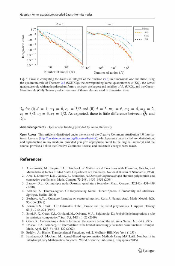
Set � = 1.2 and consider the integrand

f (x) =d∏

i=1

exp

(− ci x2i

2�2

)xmi . (5.3)

When 0 < ci < 4 and mi ∈ N for each i = 1, . . . , d, the function is in H [25,Theorems 1 and 3]. Furthermore, the Gaussian integral of this function is available inclosed form:

(2π)−d/2∫Rd

f (x) e−‖x‖2/2 dx =d∏

i=1

mi !2mi /2(mi/2)!

(�√ci

)mi +1( 1

1 + �2/ci

)(mi +1)/2

when mi are even (when they are not even, the integral is obviously zero). Figure 5shows integration error of the three methods (or, in higher dimensions, their tensorproduct versions) used in Sect. 5.4 and the kernel quadrature rule based on the nodes

123

Gaussian kernel quadrature at scaled Gauss–Hermite nodes

10 20 30

100

10−2

10−4

10−6

10−8

10−10

10−12

10−14

Number of nodes (N)

Inte

grat

ion

erro

rd = 1

101 102 103 104

Number of nodes (N)

d = 3SGHKQ

KQ

UKQ

GH

Fig. 5 Error in computing the Gaussian integral of the function (5.3) in dimensions one and three usingthe quadrature rule of Theorem 2.2 (SGHKQ), the corresponding kernel quadrature rule (KQ), the kernelquadrature rule with nodes placed uniformly between the largest and smallest of xn (UKQ), and the Gauss–Hermite rule (GH). Tensor product versions of these rules are used in dimension three

xn for (i) d = 1, m1 = 6, c1 = 3/2 and (ii) d = 3, m1 = 6, m2 = 4, m3 = 2,c1 = 3/2, c2 = 3, c3 = 1/2. As expected, there is little difference between Qk andQk .

Acknowledgements Open access funding provided by Aalto University.

Open Access This article is distributed under the terms of the Creative Commons Attribution 4.0 Interna-tional License (http://creativecommons.org/licenses/by/4.0/), which permits unrestricted use, distribution,and reproduction in any medium, provided you give appropriate credit to the original author(s) and thesource, provide a link to the Creative Commons license, and indicate if changes were made.

References

1. Abramowitz, M., Stegun, I.A.: Handbook of Mathematical Functions with Formulas, Graphs, andMathematical Tables. United States Department of Commerce, National Bureau of Standards (1964)

2. Area, I., Dimitrov, D.K., Godoy, E., Ronveaux, A.: Zeros of Gegenbauer and Hermite polynomials andconnection coefficients. Math. Comput. 73(248), 1937–1951 (2004)

3. Barrow, D.L.: On multiple node Gaussian quadrature formulae. Math. Comput. 32(142), 431–439(1978)

4. Berlinet, A., Thomas-Agnan, C.: Reproducing Kernel Hilbert Spaces in Probability and Statistics.Springer, Berlin (2004)

5. Bezhaev, A.Yu.: Cubature formulae on scattered meshes. Russ. J. Numer. Anal. Math. Model. 6(2),95–106 (1991)

6. Bonan, S.S., Clark, D.S.: Estimates of the Hermite and the Freud polynomials. J. Approx. Theory63(2), 210–224 (1990)

7. Briol, F.-X., Oates, C.J., Girolami, M., Osborne, M.A., Sejdinovic, D.: Probabilistic integration: a rolein statistical computation? Stat. Sci. 34(1), 1–22 (2019)

8. Cools, R.: Constructing cubature formulae: the science behind the art. Acta Numer. 6, 1–54 (1997)9. Driscoll, T.A., Fornberg,B.: Interpolation in the limit of increasinglyflat radial basis functions.Comput.

Math. Appl. 43(3–5), 413–422 (2002)10. Erdélyi, A.: Higher Transcendental Functions, vol. 2. McGraw-Hill, New York (1953)11. Fasshauer, G., McCourt, M.: Kernel-Based Approximation Methods Using MATLAB. Number 19 in

Interdisciplinary Mathematical Sciences. World Scientific Publishing, Singapore (2015)

123

T. Karvonen, S. Särkkä

12. Fasshauer, G.E.,McCourt,M.J.: Stable evaluation ofGaussian radial basis function interpolants. SIAMJ. Sci. Comput. 34(2), A737–A762 (2012)

13. Gautschi,W.: Orthogonal Polynomials: Computation andApproximation. NumericalMathematics andScientific Computation. Oxford University Press, Oxford (2004)

14. Kanagawa, M., Sriperumbudur, B.K., Fukumizu, K.: Convergence analysis of deterministic kernel-based quadrature rules in misspecified settings. Found. Comput. Math. (2019). https://doi.org/10.1007/s10208-018-09407-7

15. Karlin, S., Studden, W.J.: Tchebycheff Systems: With Applications in Analysis and Statistics. Inter-science Publishers, New York (1966)

16. Karvonen, T., Särkkä, S.: Fully symmetric kernel quadrature. SIAM J. Sci. Comput. 40(2), A697–A720(2018)

17. Kellog, O.D.: Orthogonal function sets arising from integral equations. Am. J. Math. 40(2), 145–154(1918)

18. Kuo, F.Y., Sloan, I.H.,Wozniakowski, H.: Multivariate integration for analytic functions with Gaussiankernels. Math. Comput. 86, 829–853 (2017)

19. Kuo, F.Y., Wozniakowski, H.: Gauss-Hermite quadratures for functions from Hilbert spaces withGaussian reproducing kernels. BIT Numer. Math. 52(2), 425–436 (2012)

20. Larkin, F.M.: Optimal approximation in Hilbert spaces with reproducing kernel functions. Math. Com-put. 24(112), 911–921 (1970)

21. Larkin, F.M.: Gaussian measure in Hilbert space and applications in numerical analysis. Rocky Mt. J.Math. 2(3), 379–422 (1972)

22. Larsson, E., Fornberg, B.: Theoretical and computational aspects of multivariate interpolation withincreasingly flat radial basis functions. Comput. Math. Appl. 49(1), 103–130 (2005)

23. Lee, Y.J., Micchelli, C.A., Yoon, J.: On convergence of flat multivariate interpolation by translationkernels with finite smoothness. Constr. Approx. 40(1), 37–60 (2014)

24. Lee, Y.J., Yoon, G.J., Yoon, J.: Convergence of increasingly flat radial basis interpolants to polynomialinterpolants. SIAM J. Math. Anal. 39(2), 537–553 (2007)

25. Minh, H.Q.: Some properties of Gaussian reproducing kernel Hilbert spaces and their implications forfunction approximation and learning theory. Constr. Approx. 32(2), 307–338 (2010)

26. Minka, T.: Deriving quadrature rules fromGaussian processes. Technical report, Statistics Department,Carnegie Mellon University (2000)

27. Mysovskikh, I.P.: On the construction of cubature formulas with fewest nodes. Sov. Math. Dokl. 9,277–280 (1968)

28. Oettershagen, J.: Construction ofOptimal CubatureAlgorithmswithApplications to Econometrics andUncertainty Quantification. PhD thesis, Institut für Numerische Simulation, Universität Bonn (2017)

29. O’Hagan, A.: Bayes–Hermite quadrature. J. Stat. Plan. Inference 29(3), 245–260 (1991)30. Pinkus, A.: Spectral properties of totally positive kernels and matrices. In: Gasca, M., Micchelli, C.A.

(eds.) Total Positivity and Its Applications. Springer, pp. 477–511 (1996)31. Rasmussen, C.E., Ghahramani, Z.: Bayesian Monte Carlo. In: Becker, S., Thrun, S., Obermayer, K.

(eds.) Advances in Neural Information Processing Systems, vol. 15, pp. 505–512 (2002)32. Richter-Dyn, N.: Properties of minimal integration rules II. SIAM J. Numer. Anal. 8(3), 497–508

(1971)33. Schaback, R.: Error estimates and condition numbers for radial basis function interpolation. Adv.

Comput. Math. 3(3), 251–264 (1995)34. Schaback, R.: Multivariate interpolation by polynomials and radial basis functions. Constr. Approx.

21(3), 293–317 (2005)35. Sommariva, A., Vianello, M.: Numerical cubature on scattered data by radial basis functions. Com-

puting 76(3–4), 295–310 (2006)36. Steinwart, I., Hush, D., Scovel, C.: An explicit description of the reproducing kernel Hilbert spaces of

Gaussian RBF kernels. IEEE Trans. Inf. Theory 52(10), 4635–4643 (2006)37. Steinwart, I., Scovel, C.: Mercer’s theorem on general domains: on the interaction between measures,

kernels, and RKHSs. Constr. Approx. 35(3), 363–417 (2012)38. Sun, H.: Mercer theorem for RKHS on noncompact sets. J. Complex. 21(3), 337–349 (2005)

Publisher’s Note Springer Nature remains neutral with regard to jurisdictional claims in published mapsand institutional affiliations.

123