1

Bit Weaving: A Non-prefix Approach to

Compressing Packet Classifiers in TCAMsChad R. Meiners Alex X. Liu Eric Torng

Abstract—Ternary Content Addressable Memories (TCAMs)have become the de facto standard in industry for fast packetclassification. Unfortunately, TCAMs have limitations of smallcapacity, high power consumption, high heat generation, and highcost. The well-known range expansion problem exacerbates theselimitations as each classifier rule typically has to be convertedto multiple TCAM rules. One method for coping with theselimitations is to use compression schemes to reduce the numberof TCAM rules required to represent a classifier. Unfortunately,all existing compression schemes only produce prefix classifiers.Thus, they all miss the compression opportunities created bynon-prefix ternary classifiers.

In this paper, we propose bit weaving, the first non-prefixcompression scheme. Bit weaving is based on the observation thatTCAM entries that have the same decision and whose predicatesdiffer by only one bit can be merged into one entry by replacingthe bit in question with *. Bit weaving consists of two newtechniques, bit swapping and bit merging, to first identify and thenmerge such rules together. The key advantages of bit weaving arethat it runs fast, it is effective, and it is composable with otherTCAM optimization methods as a pre/post-processing routine.

We implemented bit weaving and conducted experiments onboth real-world and synthetic packet classifiers. Our experimen-tal results show the following: (i) bit weaving is an effectivestand-alone compression technique (it achieves an average com-pression ratio of 23.6%) and (ii) bit weaving finds compressionopportunities that other methods miss. Specifically, bit weavingimproves the prior TCAM optimization techniques of TCAMRazor and Topological Transformation by an average of 12.8%

and 36.5%, respectively.

Index Terms—TCAM, packet classification

I. INTRODUCTION

A. Background on TCAM-Based Packet Classification

Packet classification is the core mechanism that enables

many networking devices, such as routers and firewalls, to per-

form services such as packet filtering, virtual private networks

(VPNs), network address translation (NAT), quality of service

(QoS), load balancing, traffic accounting and monitoring,

differentiated services (Diffserv), etc. The essential problem

is to compare each packet with a list of predefined rules,

Manuscript received October 17, 2009; revised January 11, 2011; acceptedJuly 8, 2011; approved by IEEE/ACM TRANSACTIONS ON NETWORK-ING Editor Isaac Keslassy. Date of publication ; date of current version . Thiswork was supported in part by the U.S. National Science Foundation underGrant Numbers CNS-0916044 and CNS-0845513. A preliminary versionof this paper titled “Bit Weaving: A Non-prefix Approach to CompressingPacket Classifiers in TCAMs” was published in the proceedings of the IEEEInternational Conference on Network Protocols (ICNP), pages 93-102, 2009.The technical report version of this paper was published in January 2009 atMichigan State University.

The authors are with the Department of Computer Science and Engineeringat Michigan State University, East Lansing, MI 48823 USA (email: mein-ersc@cse.msu.edu; alexliu@cse.msu.edu; torng@cse.msu.edu). Chad Meinersis now at MIT Lincoln Laboratory (email: chad.meiners@ll.mit.edu).

which we call a packet classifier, and find the first (i.e.,

highest priority) rule that the packet matches. Table I shows an

example packet classifier of three rules. Each rule r consists of

a predicate p(r) that describes which packets are governed by

a given rule and a decision or action d(r) that describes what

should be done with matching packets. The format of these

rules is based upon the format used in Access Control Lists

(ACLs) on Cisco routers. In this paper we use the terms packet

classifiers, ACLs, rule lists, and lookup tables interchangeably.

Rule Source IP Dest. IP Source Port Dest. Port Protocol Action

r1 1.2.3.0/24 192.168.0.1 [1,65534] [1,65534] TCP accept

r2 1.2.11.0/24 192.168.0.1 [1,65534] [1,65534] TCP accept

r3 * * * * * discard

TABLE IAN EXAMPLE PACKET CLASSIFIER

Hardware-based packet classification using Ternary Content

Addressable Memories (TCAMs) is now the de facto industry

standard [1], [2]. TCAM-based packet classification is widely

used because Internet routers need to classify every packet on

the wire. Although software based packet classification has

been extensively studied (see survey paper [3]), these tech-

niques cannot match the wire speed performance of TCAM-

based packet classification systems.

The CAM in TCAM means that TCAMs are content

addressable memory as opposed to random access memory.

As with other content addressable memories, a TCAM chip

receives a search key and returns the address of the first

TCAM entry that matches the search key in constant time

(i.e., a few clock cycles). The TCAM hardware achieves this

by comparing the search key with all its occupied entries in

parallel and then using a priority encoder circuit to isolate the

first entry that matches. The T in TCAM is short for ternary

which means each TCAM “bit” can take one of three values:

0, 1, or * which represents a don’t care value. Two ternary

strings match if their corresponding 0’s and 1’s match. TCAM-

based packet classifiers typically work as follows. First, the

TCAM is paired with an SRAM with the same number of

entries. Given a rule r, p(r) is stored as a ternary string in

TCAM entry i, and decision d(r) is stored in SRAM entry

i. When a packet arrives, the relevant packet header bits are

extracted to form the TCAM search key. The index returned

by the TCAM search is then used to find the correct decision

in the corresponding SRAM.

B. Motivation for TCAM-based Classifier Compression

Although TCAM-based packet classification is currently

the de facto standard in industry, TCAMs do have several

limitations. First, TCAM chips have limited capacity. The

largest available TCAM chip has a capacity of 72 megabits

(Mb). Smaller TCAM chips are the most popular due to

the other limitations of TCAM chips stated below. Second,

TCAMs require packet classification rule predicates to be in

ternary format. This leads to the well-known range expansion

problem, i.e., converting rule predicates to ternary format

results in a much larger number of TCAM entries, which

exacerbates the problem of limited capacity TCAMs. In a

typical rule predicate, the three fields of source and destination

IP addresses and protocol type are specified as prefixes (e.g.,

1011****) where all the *s are at the end of the ternary

string, so the fields can be directly stored in a TCAM.

However, the remaining two fields of source and destination

port numbers are specified in ranges (i.e., integer intervals such

as [1, 65534]), which need to be converted to one or more

prefixes before being stored in a TCAM. This can lead to a

significant increase in the number of TCAM entries needed to

encode a rule predicate. For example, 30 prefixes are needed to

represent the single range [1, 65534], so 30×30 = 900 TCAM

entries are required to represent the single rule predicate p(r1)in Table I. Third, TCAM chips consume lots of power. The

power consumption of a TCAM chip is about 1.85 Watts per

Mb [4]. This is roughly 30 times larger than a comparably

sized SRAM chip [5]. TCAMs consume lots of power because

every memory access searches the entire active memory in

parallel. That is, a TCAM is not just memory, but memory and

a (very fast) parallel search system. Fourth, TCAMs generate

lots of heat due to their high power consumption. Fifth, a

TCAM chip occupies a large footprint on a line card. A TCAM

chip occupies 6 times (or more) board space than an equivalent

capacity SRAM chip [5]. For networking devices such as

routers, area efficiency of the circuit board is a critical issue.

Finally, TCAMs are expensive, costing hundreds of dollars

even in large quantities. TCAM chips often cost more than

network processors [6]. The high price of TCAMs is mainly

due to their large die area, not their market size [5]. Power

consumption, heat generation, board space, and cost lead to

system designers using smaller TCAM chips than the largest

available. For example, TCAM components are often restricted

to at most 10% of an entire board’s power budget, so a 36 Mb

TCAM may not be deployable on many routers due to power

consumption reasons.

While TCAM-based packet classification is the current

industry standard, the above limitations imply that existing

TCAM-based solutions may not be able to scale up to meet

the future packet classification needs of the rapidly growing

Internet. Specifically, packet classifiers are growing rapidly in

size and width due to several causes. First, the deployment

of new Internet services and the rise of new security threats

lead to larger and more complex packet classification rule sets.

While traditional packet classification rules mostly examine

the five standard header fields, new classification applications

begin to examine additional fields such as classifier-id, proto-

col flags, ToS (type of service), switch-port numbers, security

tags, etc. Second, with the increasing adoption of IPv6, the

number of bits required to represent source and destination IP

address will grow from 64 to 256. The size and width growth

of packet classifiers puts more demand on TCAM capacity,

power consumption, and heat dissipation.

To address the above TCAM limitations and ensure the

scalability of TCAM-based packet classification, we study the

following TCAM-based classifier compression problem: given

a packet classifier, we want to efficiently generate a semanti-

cally equivalent packet classifier that requires fewer TCAM

entries. Note that two packet classifiers are (semantically)

equivalent if and only if they have the same decision for every

packet. TCAM-based classifier compression helps to address

the limited capacity of deployed TCAMs because reducing

the number of TCAM entries effectively increases the fixed

capacity of a chip. Reducing the number of rule predicates

in a TCAM directly reduces power consumption and heat

generation because the energy consumed by a TCAM grows

linearly with the number of ternary rule predicates it stores

[7]. Finally, TCAM-based classifier compression lets us use

smaller TCAMs, which results in less power consumption, less

heat generation, less board space, and lower hardware cost.

C. Limitations of Prior Art

All prior TCAM-based classifier compression schemes (i.e.,

[8]–[13]) suffer from one fundamental limitation: they only

produce prefix classifiers, which means they all miss some

opportunities for compression. A prefix classifier is a classifier

in which every rule predicate is a prefix rule. In a prefix rule,

each field is specified as a prefix bit string (e.g., 01**) where *s

all appear at the end. In a ternary rule, each field is a ternary bit

string (e.g., 0**1) where * can appear at any position. Every

prefix rule is a ternary rule, but not vice versa. Because all

previous compression schemes can only produce prefix rules,

they miss the compression opportunities created by non-prefix

ternary rules.

D. Our Bit Weaving Approach

In this paper, we propose bit weaving, a new TCAM-based

classifier compression scheme that is not limited to producing

prefix classifiers. The basic idea of bit weaving is simple:

adjacent TCAM entries that have the same decision and have

a hamming distance of one (i.e., differ by only one bit) can be

merged into one entry by replacing the bit in question with *.

Bit weaving applies two new techniques, bit swapping and bit

merging, to first identify and then merge such rules together.

Bit swapping first cuts a rule list into a series of partitions.

Within each partition, a single permutation is applied to each

rule’s predicate to produce a reordered rule predicate, which

forms a single prefix where all *’s are at the end of the rule

predicate. This single prefix format allows us to use existing

dynamic programming techniques [9], [13] to find a minimal

TCAM table for each partition in polynomial time. Bit merging

then finds and merges mergeable rules from each partition.

After bit merging, we revert all ternary strings back to their

original bit permutation to produce the final TCAM table.

We name our solution bit weaving because it manipulates bit

ordering in a ternary string much like a weaver manipulates

the position of threads.

The example in Figure 1 shows that bit weaving can further

compress a minimal prefix classifier. The input classifier has 5

prefix rules with three decisions (0, 1, and 2) over two fields F1

and F2, where each field has two bits. Bit weaving compresses

this minimal prefix classifier with 5 rules down to 3 ternary

rules as follows. First, it cuts the input prefix classifier into two

partitions which are the first two rules and the last three rules,

respectively. Second, it swaps bit columns in each partition to

make the two-dimensional rules into one-dimensional prefix

rules. In this example, in the second partition, the second

and the fourth columns are swapped. We call the above

two steps bit swapping. Third, we treat each partition as

a one-dimensional prefix rule list and generate a minimal

prefix representation. In this example, the second partition is

minimized to 2 prefix rules. Fourth, in each partition, we detect

and merge rules that can be merged. In the first partition, the

two rules are merged. We call this step bit merging. Finally,

we revert each partition back to its original bit order. In this

example, for the second partition after minimization, we swap

the second and the fourth columns again to recover the original

bit order. The final output is a ternary packet classifier with

only 3 rules.

Fig. 1. Example of the bit weaving approach

E. Our Contributions

Our bit weaving approach has many significant properties.

First, it is the first TCAM-based classifier compression method

that can create non-prefix classifiers for classifiers with more

than 2 decisions. Most previous compression methods gener-

ate only prefix classifiers [11], [13]–[15]. This restriction to

prefix format may miss important compression opportunities.

The only exception is McGeer and Yalagandula’s classifier

compression scheme, which works only on classifiers with

2 decisions [16]. Note that the technical report version of

our paper was published before [16]. Second, it is the first

efficient compression method with a polynomial worst-case

running time with respect to the number of fields in each rule.

Third, it is orthogonal to other techniques, which means that

it can be run as a pre/post-processing routine in combination

with other compression techniques. In particular, bit weaving

complements TCAM Razor [13] nicely. In our experiments on

real-world classifiers, bit weaving outperforms TCAM Razor

on classifiers that do not have significant range expansion.

Fourth, unlike TCAM Razor, it may be used on partially

defined classifiers, so bit weaving can be used in more appli-

cations than TCAM Razor. Fifth, it supports fast incremental

updates to classifiers.

F. Summary of Experimental Results

We implemented bit weaving and conducted experiments

on both real-world and synthetic packet classifiers. Our experi-

mental results show that bit weaving is an effective stand-alone

compression technique as it achieves an average compression

ratio of 23.6% and that bit weaving finds compression op-

portunities that other methods miss. Specifically, bit weaving

improves the prior TCAM optimization techniques of TCAM

Razor [13], and Topological Transformation [17] by an aver-

age of 12.8% and 36.5%, respectively.

The rest of this paper proceeds as follows. We start by

reviewing related work in Section II. We define bit swapping

in Section III and bit merging in Section IV. In Section V,

we discuss how bit weaving supports incremental updates,

how bit weaving can be composed with other compression

methods, and the complexity bounds of bit weaving. We show

our experimental results on both real-life and synthetic packet

classifiers in Section VII, and we give concluding remarks in

Section VIII.

II. RELATED WORK

TCAM-based packet classification systems have been

widely deployed due to their O(1) classification time. This

has led to a significant amount of work that explores ways to

efficiently store packet classifiers within TCAMs. Prior work

falls into three broad categories: classifier compression, range

encoding, and circuit and hardware modification.

A. Classifier Compression

Classifier compression converts a given packet classifier

to another semantically equivalent packet classifier that re-

quires fewer TCAM entries. Several classifier compression

schemes have been proposed [8]–[11], [13], [14]. The work

is either focused on one-dimensional and two dimensional

packet classifiers [8]–[10], or it is focused on compressing

packet classifiers with more than 2 dimensions [11], [13]–[15].

Liu and Gouda proposed the first algorithm for eliminating

all the redundant rules in a packet classifier [14], and we

presented a more efficient redundancy removal algorithm [15].

Dong et al. proposed schemes to reduce range expansion by

repeatedly expanding or trimming ranges to prefix boundaries

[11]. Their schemes use redundancy removal algorithms [14]

to test whether each modification changes the semantics of the

classifier. We proposed a greedy algorithm that finds locally

minimal prefix solutions along each field and combines these

solutions into a smaller equivalent prefix packet classifier [13].

Bit weaving differs from these previous efforts in that it

is the first polynomial classifier minimization algorithm that

produces equivalent non-prefix packet classifiers given an arbi-

trary number of fields and decisions. McGeer and Yalagandula

proved the NP-hardness of ternary classifier minimization and

proposed an algorithm that finds an optimal ternary classifier

using using circuit minimization algorithms [16]. However,

this algorithm has an exponential complexity in terms of the

number of rules in a classifier. As such, the authors proposed

three approximation heuristics; unfortunately, the running time

of their approximation algorithms is often too slow as they do

not guarantee a polynomial running time - sometimes hours

or unable to finish, and their heuristics are only applicable

to classifiers with two decisions - but classifiers with four

decisions (accept, accept with logging, discard, and discard

with logging) are very common. In contrast, bit weaving is the

first algorithm whose worst-case running time is polynomial

with respect to the number of fields and bits within a classifier.

B. Range Encoding

Range encoding schemes cope with range expansion by

developing a new representation for important packets and

intervals. For example, a new representation for interval

[1, 65534] may be developed so that this interval can be

represented with one TCAM entry rather than 900 prefix

entries. Previous range encoding schemes fall into two cat-

egories: database independent encoding schemes [1], [18],

where each rule predicate is encoded according to standard

encoding scheme, and database dependent encoding schemes

[17], [19]–[23], where the encoding of each rule predicate

depends on the intervals present within the classifier. Some

prior range encoding schemes do create non-prefix fields [18];

however, range encoding schemes in general require extra

hardware or more per packet processing time in order to

transform packet fields on the fly into the new representation.

This makes range encoding schemes different than classifier

compression schemes such as bit weaving which do not require

any modifications to hardware or more per packet processing

time.

C. Circuit and Hardware Modification

Spitznagel et al. proposed adding comparators at each

entry level to better accommodate range matching [24]. While

this research direction is important, our contribution does

not require circuit-level modifications to hardware. Zheng et

al. developed load balancing algorithms for TCAM based

systems to exploit chip level parallelism to increase classifier

throughput with multiple TCAM chips without having to copy

the complete classifier to every TCAM chip [25], [26]. This

work may benefit from bit weaving since fewer rules would

need to be distributed among the TCAM chips.

III. BIT SWAPPING

In this section, we present a new technique called bit

swapping. It is the first part of our bit weaving approach.

A. Prefix Bit Swapping Algorithm

Definition III.1 (Bit-swap). A bit-swap β for a length m

ternary string t is a permutation of the numbers 1 through

m. We apply β to t by permuting the bits of t according to β

and denote the resulting permuted ternary string by β(t). 2

For example, if β is permutation 312 and string t is 0∗1,

then β(t) = 10∗. For any length m string, there are m!different bit-swaps.

Definition III.2 (Prefix bit-swap). Bit-swap β for ternary

string t is a prefix bit-swap for t if the permuted string β(t)is in prefix format. We use P (t) to denote the set of prefix

bit-swaps for t: specifically, the bit-swaps that move the ∗ bits

of t to the end of the string.

A bit-swap β can be applied to a list ℓ of ternary strings

〈t1, . . . , tn〉 where ℓ is typically a list of consecutive rules in

a packet classifier. The resulting list of permuted strings is

denoted as β(ℓ). Bit-swap β is a prefix bit-swap for ℓ if β is a

prefix bit-swap for every string ti in list ℓ for 1 ≤ i ≤ n. Let

P (ℓ) denote the set of prefix bit-swaps for list ℓ. It follows

that P (ℓ) = ∩ni=1P (ti).

Prefix bit-swaps are useful for two main reasons. First, we

can use algorithms [8], [9], [27] that can optimally minimize

prefix rule lists. These polynomial algorithms requires the

input to be prefix rules. To our best knowledge, until now there

is no polynomial algorithm that can optimally minimize non-

prefix rule lists. Thus, converting rules lists into prefix rules

is a necessary step to minimize them. Second, prefix format

facilitates the second key idea of bit weaving, bit merging

(Section IV). Specifically, we exploit special properties of pre-

fix format rules to identify candidate rules that can be merged

together without changing the semantics of the classifier. After

bit merging, the classifier is reverted to its original bit order,

which typically results in a non-prefix field classifier.

Unfortunately, many lists of strings ℓ have no prefix bit-

swaps which means that P (ℓ) = ∅. For example, the list

〈0∗, ∗0〉 does not have a prefix bit-swap. We now give the

necessary and sufficient conditions for P (ℓ) 6= ∅ after defining

the following notation.

Given length m ternary strings x and y, let x[i] and y[i]denote the ith ternary bit in x and y, respectively. Let M(x)denote the set of length m binary strings that ternary string x

ternary matches. We define the relation x ∩ y to be shorthand

for M(x) ∩ M(y), the relation x ⊆ y to be shorthand for

M(x) ⊆ M(y), and the relation x ⊑ y to be shorthand for

{i | x[i] = ∗} ⊆ {j | y[j] = ∗}. For example, 0*1 ∩ 1** = ∅,

0*1 ⊑ 1**, and 0*1 6⊆ 1** whereas 0*0 ∩ 0** = 0*0, 0*0 ⊑0**, and 0*0 ⊆ 0**.

Definition III.3 (Cross Pattern). Two ternary strings t1 and

t2 form a cross pattern if and only if (t1 6⊑ t2)∧ (t2 6⊑ t1). In

such cases, we say that t1 crosses t2. 2

We first observe that bit swaps have no effect on whether

or not two strings cross each other.

Observation III.1. Given two ternary strings, t1 and t2, and

a bit-swap β, t1 ⊆ t2 if and only if β(t1) ⊆ β(t2), and t1 ⊑ t2if and only if β(t1) ⊑ β(t2). 2

Theorem III.1. Given a list ℓ = 〈t1, . . . , tn〉 of n ternary

strings, P (ℓ) 6= ∅ if and only if no two ternary strings ti and

tj (1 ≤ i < j ≤ n) cross each other. 2

Proof: (implication) It is given that there exists a prefix

bit-swap β ∈ P (ℓ). Suppose that string ti crosses string tj .

According to Observation III.1, prefix ternary string β(ti)crosses prefix ternary β(tj). However, it is impossible for two

prefix strings to cross each other since all the *’s are at the

end of both strings. This is a contradiction and the implication

follows.

(converse) It is given that no two ternary strings cross each

other. It follows that we can impose a total order on the ternary

strings in ℓ using the relation ⊑. Note, there may be more than

one total order if ti ⊑ tj and tj ⊑ ti for some values of i

and j. Let us reorder the ternary strings in ℓ according to this

total order; that is, t′1 ⊑ t′2 ⊑ · · · ⊑ t′n−1 ⊑ t′n. Any bit

swap that puts the ∗ bit positions of t′1 last, preceded by the

∗ bit positions of t′2, . . . , preceded by the ∗ bit positions of

t′n, finally preceded by all the remaining bit positions will be

a prefix bit-swap for ℓ. Thus, the result follows.

Theorem III.1 gives us a simple algorithm for detecting

whether a prefix bit-swap exists for a list of ternary strings. If

a prefix bit-swap exists, the proof of Theorem III.1 gives us

a simple algorithm for constructing a prefix bit-swap. That is,

we simply sort ternary bit positions in increasing order by the

number of ternary strings that have a ∗ in that bit position.

Figure 2(a) shows three ternary strings and Figure 2(b) shows

the resulting strings after bit swapping.

Fig. 2. Example of bit-swapping

B. Minimal Cross-Free Classifier Partitioning Algorithm

Given a classifier C, if P (C) = ∅, we treat classifier C as

a list of ternary strings by ignoring the decision of each rule.

We cut C into partitions where each partition has no cross

patterns and thus has a prefix bit-swap.

Given an n-rule classifier C = 〈r1, . . . , rn〉, a partition P

on C is a list of consecutive rules 〈ri, . . . , rj〉 in C for some i

and j such that 1 ≤ i ≤ j ≤ n. A partitioning, P1, . . . ,Pk, of

C is a series of k partitions on C such that the concatenation

of P1, . . . ,Pk is C. A partitioning is cross-free if and only if

each partition has no cross patterns. Given a classifier C, a

cross-free partitioning with k partitions is minimal if and only

if any partitioning of C with k− 1 partitions is not cross-free.

In bit swapping, we find a minimal cross-free partitioning

for a given classifier and then apply independent prefix bit-

swaps to each partition. We choose to find a minimal cross-

free partitioning for a given classifier because each partition

becomes a separate optimization problem. Specifically, in bit

merging, we can only merge rules from the same partition.

By reducing the total number of partitions, we increase the

number of merging opportunities per partition.

Our algorithm for finding a minimal cross-free partitioning

is depicted in Algorithm 1. At any time, we have one active

partition. The initial active partition is the last rule of the

classifier. We consider each rule in the classifier in reverse

order and attempt to add it to the active partition. If the current

rule crosses any rule in the active partition, that partition is

completed, and the active partition is reset to contain only the

new rule. Our algorithm is written so that it processes rules

from last to first. It obviously can be easily modified to process

rules from first to last.

Theorem III.2. Given a classifier C and a cross-free parti-

tioning P1, . . . ,Pk formed by our algorithm. Then P1, . . . ,Pk

is a minimal cross-free partitioning. 2

Proof: To create k partitions, our algorithm identifies k−1cross patterns. Any partitioning with only k−1 partitions must

place both rules from one of the cross patterns into the same

partition and thus cannot be cross free.

Algorithm 1: Find a minimal partition

Input: A list of n rules 〈r1, . . . , rn〉 where each rule has

b bits.

Output: A list of partitions.

Let P be the current partition (empty list), and L be a

list of partitions (empty);

for i := n to 1 do

if ri introduces a cross pattern in P then

Append P to the head of L;

P := 〈ri〉;else

Append ri to the head of P ;

return L;

The core operation in our cross-free partitioning algorithm

is checking whether or not two ternary strings x and y cross

each other. This check requires computing the negation of x ⊑y∧y ⊑ x. This can be performed in constant time using bitmap

representations of sets.

Figure 3 shows the execution of our bit weaving algorithm

on an example classifier. We describe the bit swapping portion

of that execution. The input classifier has 10 prefix rules with

three decisions (0, 1, and 2) over two fields F1 and F2, where

F1 has two bits, and F2 has six bits. We begin by constructing

a minimal cross-free partitioning of the classifier by starting at

the last rule and working upward. We find that the seventh rule

crosses the eighth rule. This results in splitting the classifier

into two partitions. Second, we perform bit swapping on each

partition, which converts each partition into a list of one-

dimensional prefix rules.

C. Partial List Minimization Algorithm

We now describe how to minimize each bit-swapped parti-

tion where we view each partition as a one-dimensional prefix

classifier. If a one-dimensional prefix classifier is complete

(i.e., any packet has a matching rule in the classifier), we can

use the algorithms in [8], [9] to produce an equivalent minimal

prefix classifier. However, the classifier in each partition is

typically incomplete; that is, there exist packets that will not

be classified by any rule in the partition. There are two reasons

why packets will not be classified by any rule in the partition.

First, if any of the first k − 1 partitions are complete, all

later partitions can be deleted without changing the classifier

semantics given the first match semantics of TCAMs. Thus we

can assume that each of the first k−1 partitions do not assign

a decision to some packets. Second, for any of the final k− 1partitions, many packets are classified by earlier partitions and

thus will not be classified by the given partition even though

those packets may match rules in the given partition. We now

describe how we minimize the one-dimensional classifier of

each bit-swapped partition.

** 100000 1** 100010 1** 100100 1** 100110 1** 101000 1 ** 110000 1 ** 111000 1

01 ****** 21* ****** 2** ****** 0

swappingBit

00****** 0******** 2

MergingBit

100000** 1100010** 1100100** 1100110** 1101000** 1110000** 1111000** 1

01****** 21******* 2******** 0

00****** 0******** 2

Recovery

00****** 0******** 2

100**0** 11**000** 1

**100**0 1**1**000 1

100000** 1100010** 1100100** 1100110** 1101000** 1110000** 1111000** 1

Minimizing

F1 F2

Bit

Fig. 3. Applying bit weaving algorithm to an example classifier

We adapt the algorithm that minimizes a weighted one-

dimensional prefix classifier in [27] to minimize the partial

classifier that corresponds to a given bit-swapped partition. A

weighted classifier C with n rules is one in which each rule

decision di has a cost (weight) Cost(di ), and the weighted

cost of C with n rules is simply the sum of the costs of each

rule decision in C.

Let L be the partial classifier that corresponds to

a bit-swapped partition that we want to minimize. Let

{d1, d2, · · · , dz} be the set of all the decisions of the rules

in L. We assign each of these decisions a weight of 1.

We now add rules and decisions to address the two different

reasons why packets might not be classified by L. We first

show how we can use the existence of earlier partitions to

further compress L. Consider Table II which contains two

partitions where partition 1’s bit swap is changed to partition

2’s bit swap in order to directly compare the predicates of

each partition’s rules. If we ignore the existence of the first

partition, the second partition is minimal. However, given that

the rule 0111 → d does occur before partition 2, we can

rewrite partition 2’s three rules as the single rule 0∗ ∗ ∗ → a.

We call leveraging the existence of earlier partitions when

minimizing a given partition prefix shadowing.

Partition 1

∗000 → d ⇒ ∗000 → d

0111 → d ⇒ 0111 → d

Partition 2

010∗ → a

0110 → a ⇒ 0∗ ∗ ∗ → a

00∗∗ → a

TABLE IITHE SECOND PARTITION BENEFITS FROM THE PREFIX SHADOW OF THE

FIRST PARTITION

In prefix shadowing, we first compute a set of prefixes L̂

using L’s bit swap that are covered by earlier partitions that

will be added to L. Computing L̂ is nontrivial for two reasons.

First, L’s bit swap is different than bit swaps from earlier

partitions. Second, adding too many prefixes to L̂ may lead to

a cross pattern in L whereas adding too few prefixes to L̂ leads

to no increase in compression. Next, for each prefix p ∈ L̂, we

append a new rule p → dz+1 to the front of L where decision

dz+1 is a new decision that does not appear in L. Let L1 be

the resulting classifier. We set the cost of dz+1 to 0 because all

rules with decision dz+1 are free. Specifically, prefixes with

decision dz+1 are covered by prior partial classifiers which

makes them redundant. Thus, all rules with decision dz+1 can

be safely removed from L1 without changing the semantics

of the entire classifier. The effectiveness of prefix shadowing

is highly dependent on the input classifiers. In our real life

classifiers, we found no benefit from prefix shadowing, so no

results are reported for prefix shadowing.

We now handle packets that do not match any rules in L or

L1 because they are classified by later partitions. We create a

default rule r∗ that matches all packets and assign it decision

dz+2 and give it a weight of F , the number of distinct packet

headers. This rule is appended to the end of L1 to create a final

classifier L2. Finally, we run the weighted one-dimensional

prefix list minimization algorithm in [27] on L2. Given our

weight assignment for decisions, we know the final rule of

the resulting classifier L3 will still be r∗ and that this rule

will be the only one with decision dz+2. Remove this final

rule r∗ from L3, and the resulting classifier is the minimal

partial classifier that is equivalent to L.

IV. BIT MERGING

In this section, we present bit merging, the second part

of our bit weaving approach. The fundamental idea behind

bit merging is to repeatedly find two ternary strings within a

partition that differ only in one bit and replace them with a

single ternary string where the differing bit is ∗.

A. Definitions

Definition IV.1 (ternary adjacent). Two ternary strings t1 and

t2 are ternary adjacent if they differ only in one bit, i.e., their

hamming distance [28] is one. The ternary string produced by

replacing the one differing bit by a ∗ in t1 (or t2) is called

the ternary cover of t1 and t2.

For example, 00∗ and 01∗ are ternary adjacent and 0∗∗ is

their ternary cover.

Definition IV.2 (mergeable). Two rules ri and ri+1 are

mergeable in a classifier C if they satisfy the following three

conditions: (1) Their predicates p(ri) and p(rj) are ternary

adjacent. (2) They share the same decision d(ri) = d(rj).(3) They are positionally adjacent within the C; that is, rule

ri+1 immediately follows rule ri within the C. The merger of

two mergeable rules ri and ri+1 is a ternary cover rule r′

such that p(r′) is the ternary cover of p(ri) and p(ri+1) and

d(r′) = d(ri) = d(ri+1).

Given any classifier C and two mergeable rules ri and ri+1

within C, it is obvious that replacing two mergeable rules by

their ternary cover rule does not change the semantics of the

resulting classifier.

Definition IV.3 (Classifier permutations). For any classifier C,

let {C} denote the set of all classifiers that are permutations

of the rules in C that are semantically equivalent to C.

Definition IV.4 (bit mergeable). Two rules ri and rj are bit

mergeable in a classifier C if they are mergeable within some

classifier C′ ∈ {C}.

The basic idea of bit merging is to repeatedly find two rules

in the same bit-swapped partition that are bit mergeable and

replace them with their ternary cover rule. We do not consider

bit merging rules from different bit-swapped partitions because

any two bits from the same column in the two bit-swapped

rules may correspond to different columns in the original rules.

We now present a bit merging algorithm for minimum prefix

classifiers in Algorithm 2.

B. Bit Merging Algorithm (BMA)

1) Prefix Decision Chunks: We first focus on finding the

appropriate permuted classifiers within {C} that facilitate

identifying bit mergeable rules. For any one-dimensional prefix

classifier C, let Cs denote the prefix classifier formed by

sorting all the rules in C in non-increasing order of prefix

length where the prefix length of a rule is the number of ternary

bits that are not *. We prove that C ≡ Cs which means that

Cs ∈ {C} if C is a one-dimensional minimum prefix classifier

in Theorem IV.1.

Before we introduce and prove Theorem IV.1, we first

present Lemma IV.1. A rule r is upward redundant if and

only if there are no packets whose first matching rule is r

[14]. Clearly, upward redundant rules can be removed from a

classifier with no change in semantics.

Lemma IV.1. For any two rules ri and rj (i < j) in a prefix

classifier 〈r1, · · · , rn〉 that has no upward redundant rules,

p(ri) ∩ p(rj) 6= ∅ if and only if p(ri) ⊂ p(rj). 2

Proof: (Implication): We are given that p(ri) ∩ p(rj) 6=∅. Since p(ri) and p(rj) are prefix strings, this means that

p(ri) = p(rj) or p(rj) ⊂ p(ri) or p(ri) ⊂ p(rj). Because

both p(ri) = p(rj) and p(rj) ⊂ p(ri) lead to the contradiction

that rj is upward redundant, it follows that p(ri) ⊂ p(rj).

(Converse): We are given that p(ri) ⊂ p(rj). If p(ri) ∩p(rj) = ∅, then p(ri) = ∅ which leads to the contradiction

that ri is upward redundant. Thus, p(ri) ∩ p(rj) 6= ∅.

Theorem IV.1. For any one-dimensional minimum prefix

packet classifier C, we have C ≡ Cs. 2

Proof: Consider any two rules ri, rj (i < j) in C. If the

predicates of ri and rj do not overlap (i.e., p(ri)∩p(rj) = ∅),

we can change the relative order between ri and rj without

changing the semantics of the given classifier. If the predicates

of ri and rj do overlap (i.e., p(ri)∩p(rj) 6= ∅), then according

to Lemma IV.1, we have p(ri) ⊂ p(rj). This means that p(ri)is strictly longer than p(rj). This implies that ri is also listed

before rj in Cs. Since the relative order of all pairs of rules

whose predicates overlap is identical in C and Cs, the result

follows.

Based on Theorem IV.1, given a minimum sized prefix bit-

swapped partition, we first sort the rules in decreasing order

of their prefix length. We next partition the rules into prefix

chunks based on their prefix length. By Theorem IV.1, the

order of the rules within each prefix chunk is irrelevant. Thus,

we know that we can permute the rules within a prefix chunk

so that any two rules from a prefix chunk are positionally

adjacent without changing the semantics of the classifier. We

next partition the rules into prefix decision groups where the

rules in a prefix decision group belong to the same prefix

chunk and have the same decision. Any two rules that belong

to the same prefix decision group whose predicates are ternary

adjacent are bit mergeable. Within a given prefix chunk, we

arbitrarily order the prefix decision chunks.2) Algorithm and Properties: The bit merging algorithm

(BMA) works as follows. BMA takes as input a minimum,

possibly incomplete prefix classifier C that corresponds to a

cross-free partition generated by bit swapping. BMA first cre-

ates classifier Cs by sorting the rules of C in decreasing order

of their prefix length and partitions Cs into prefix chunks.

Second, BMA partitions each prefix chunk into prefix decision

chunks. BMA then processes these prefix decision chunks in

the order they appear within Cs by performing several passes

over each prefix decision chunk. In each pass, BMA checks

every pair of rules to see if they are mergeable. The rules that

are not mergeable with any other rule in the prefix decision

chunk are returned as part of the output classifier. The ternary

cover rules of mergeable rules are processed in the next pass

after duplicate copies of ternary cover rules are eliminated.

BMA finishes processing the current prefix decision chunk

when no new ternary cover rules are generated in a pass. Let

C′ denote the output of the algorithm.

Figure 4 demonstrates how BMA works. On the leftmost

side is the first partition from Figure 3, all of which belong to

the same prefix decision chunk. On the first pass, eight ternary

cover rules are generated from the original seven rules and no

unmergeable rules are returned at this time. For example, the

ternary cover rule of the top two rules is the rule 1000*0**

→ 1. In the second pass, two unique ternary cover rules are

generated and no unmergeable rules are returned. Finally, in

the third pass, no mergeable rules are identified, so these two

unmergeable rules are returned as BMA finishes processing

this prefix decision chunk. If there were more prefix decision

chunks in this partition, BMA would proceed to the next

prefix decision chunk. BMA is specified more precisely in

Algorithm 2.

Fig. 4. Example of Bit Merging Algorithm Execution

Algorithm 2: Bit Merging Algorithm

Input: A minimum prefix classifier C that corresponds to

a bit-swapped cross-free partition.

Output: A semantically equivalent ternary classifier C′.

Initalize Output := ∅;

First create classifier Cs sorted in decreasing order of

prefix length;

Partition Cs into prefix decision chunks;

Create an ordered list of these prefix decision chunks

C = c1, c2, . . . , cj where the rules in ci precede the rules

in cj in Cs;

for i := 1 to j do

Rules := ci;

Unmerged := Rules;

Covers := ∅;

while Rules 6= ∅ do

for each pair of rules r′ and r′′ in Rules do

if r′ and r′′ are mergeable thenAdd the ternary cover rule of r′ and r′′ to

Covers;

Unmerged := Unmerged − {r′, r′′};

Remove duplicate rules from Covers;

Append Unmerged to Output;

Rules := Covers;

Unmerged := Covers;

Covers := ∅;

return Output;

The correctness of this algorithm, C′ ≡ C, is guaranteed

because we only combine bit mergeable rules. We now prove

that BMA terminates with no bit mergeable rules (Theorem

IV.2).

We first analyze how BMA processes each prefix decision

chunk by the number of passes performed. In each pass, the

resulting ternary cover rules generated have one more * in their

predicates than the mergeable rules that they replace. Suppose

BMA uses z passes on a specific prefix decision chunk c.

Consider a ternary cover rule r introduced in pass 1 ≤ i ≤z − 1 (no new rules are added in the final pass z). Then r

has i extra *’s in its predicate than the original prefix rules

that formed this group. We define the prefix set of r to be

the set of 2i distinct rules r′ that are identical to r except

the predicates of these rules r′ have 0 or 1 in the ternary

bit positions of the i new *’s in r’s predicate. For example,

consider Figure 4. The rule 1000*0** → 1 introduced in pass

1 has one additional * and its prefix set is {100000** → 1,

100010** → 1} whereas rule 100**0** → 1 introduced in

pass 2 has two additional *’s and its prefix set is {100000**

→ 1, 100010** → 1, 100100** → 1, 100110** → 1}.

Lemma IV.2. Consider any prefix decision chunk in Cs.

Consider any rule r that is added in the ith pass of BMA

on this group. Then the original group must include all 2i

members of r’s prefix set.

Proof: We prove this by induction on i. The base case

is i = 1. This means that r is the ternary cover rule of two

original prefix rules r′ and r′′ and the base case follows.

Now assume the lemma holds for any i where i ≥ 1. We

show it applies to i + 1. Suppose that r is introduced in the

i + 1st pass and is the ternary cover rule for rules r′ and

r′′ which were introduced in the ith pass. By our induction

hypothesis, the original group must include the entire prefix

sets for both r′ and r′′. The union of these two prefix sets is

exactly the prefix set for r, and the inductive case follows.

Lemma IV.3. Consider any prefix decision chunk in Cs that

includes all 2i members of some rule r’s prefix set where i ≥ 1.

Then rule r will be introduced in the ith pass of BMA.

Proof: We prove this by induction on i. The base case is

i = 1. It is given that the prefix decision chunk contains the

21 = 2 rules r0 and r1 that belong to r’s prefix set where r0’s

predicate has a 0 in place of the first * of r’s predicate and

r1’s predicate has a 1 in place of the first * of r’s predicate.

By definition of a prefix set and prefix decision chunk, this

means r is the ternary cover rule for r0 and r1. Thus, r will be

introduced in the 1st pass of BMA and the base case follows.

Now assume the lemma holds for any i where i ≥ 1. We

show it applies to i+ 1. It is given the prefix decision chunk

contains the 2i+1 rules that belong to r’s prefix set. Define r0and r1 to be the two rules that are identical to r except r0’s

predicate has a 0 in place of the first * of r’s predicate and

r1’s predicate has a 1 in place of the first * of r’s predicate.

It follows that the prefix decision chunk contains the 2i rules

that belong to r0’s prefix set and the 2i rules that belong to

r1’s prefix set. By our induction hypothesis, this means r0 and

r1 will be introduced in the ith pass of BMA. Furthermore, r

is the ternary cover rule of r0 and r1, so r will be introduced

in the i+1st pass of BMA and the inductive case follows.

Lemma IV.4. Consider any rule r ∈ C′ that was introduced

by BMA when processing a prefix decision chunk with a length

k prefix. The kth ternary bit of r must be 0 or 1, not ∗.

Proof: Suppose a rule r was formed that had a ∗ in the

kth ternary bit. By Lemma IV.2, all the members of r’s prefix

set were in the prefix decision chunk. This implies there must

be two bit mergeable rules in CS that differ only in their kth

ternary bits in the prefix decision chunk. This implies that CS

is not a minimal prefix classifier since it could have merged

these two rules into one prefix rule. This is a contradiction

and the result follows.

Theorem IV.2. The output of BMA, C′, contains no pair of

bit mergeable rules.

Proof: We first focus on a prefix decision chunk c. Let

Oc be the set of rules generated by BMA when processing c.

Lemmas IV.2 and IV.3 ensure there are no bit mergeable rules

within Oc.

We now prove that any two rules from different prefix

decision chunks cannot be merged. We first observe that

two rules from different prefix decision chunks but the same

prefix chunk are not bit mergeable because they have different

decisions. Thus, we now focus on two rules ri and rj from

different prefix chunks in C′ but with the same decision.

Suppose ri is from the prefix chunk of length ki and rj is

from the prefix chunk of length kj where ki > kj . By Lemma

IV.4, the ki-th bit of ri’s predicate must be 0 or 1. Because

ki > kj , the ki-th bit of rj’s predicate must be ∗. Thus, if riand rj are bit mergeable, then ri and rj should only differ in

the ki-th bit of their predicates, which means p(ri) ⊂ p(rj).This implies the ternary cover rule of ri and rj is simply rule

rj . We cannot replace rule ri and rj with simply one copy of

rj as this contradicts the minimality of Cs. That is, this would

be equivalent to eliminating at least one of the rules in ri’s

prefix set from Cs.

Continuing the example in Figure 3, we perform bit merging

on both partitions to reduce the first partition to two rules.

Finally, we revert each partition back to its original bit order.

After reverting each partition’s bit order, we recover the

complete classifier by appending the partitions together. In

Figure 3, the final classifier has four rules.V. DISCUSSION

A. Redundancy Removal

Our bit weaving algorithm uses the redundancy removal

procedure [14] as both the preprocessing and postprocessing

step. We apply redundancy removal at the beginning because

redundant rules may introduce more cross patterns. We apply

redundancy removal at the end because our incomplete 1-

dimensional prefix list minimization algorithm may introduce

redundant rules across different partitions.

B. Incremental Classifier Updates

Classifier rules periodically need to be updated when net-

working services change. When classifiers are updated man-

ually by network administrators, timing is not a concern and

rerunning the fast bit weaving algorithm will suffice. When

classifiers are updated automatically in an incremental fashion,

fast updates may be very important.

Our general approach to performing fast incremental up-

dates (the insertion, deletion, or modification of one rule) that

may occur anywhere within the classifier is as follows. First,

we locate the cross-free partition where the change occurs by

consulting a precomputed list of all rules in each partition.

Then we rerun the bit weaving algorithm on the affected

partition. This may divide the affected partition into at most

three cross-free partitions if the newly inserted or modified

rule introduces cross patterns with rules both before and after

it in the affected partition. Note that deleting a rule never

introduces cross patterns. Finally, we update the precomputed

list of all rules in each partition.

In some settings, it is unlikely that incremental updates will

occur anywhere within the classifier because it is difficult to

understand the impact of a newly inserted rule at an arbitrary

location within the classifier since that rule’s application is

limited by all previous rules in the classifier. In such cases,

rules are typically inserted at a fixed position within the

original classifier; for example, after the tenth rule. This

scenario is supported by a private communication from a

researcher that works at a major internet service provider.

To perform even faster incremental updates where rule

insertions occur at a fixed position within the classifier, we

adapt our bit swapping partitioning algorithm as follows. We

process the rules that appear before the fixed insertion location

in the initial classifier from first to the insertion point stopping

just prior to the insertion point. We process the rules that

appear after the fixed insertion point in the initial classifier

from last to the insertion point. This may lead to one more

partition than is completely necessary. Finally, we confine

inserted rules to their own partition.

The experimental data used in Section VII indicates that

only 2.7% of partitions have more than 32 rules and 0.6% of

partitions have more than 128 rules for real life classifiers. For

synthetic classifiers, these percentages are 17.3% and 0.9%,

respectively. For these classifiers, incremental classifier up-

dates are fast and efficient. To further evaluate the incremental

update times, we divided each classifier into a top half and a

bottom half. We constructed a classifier for the bottom half and

then incrementally added each rule from the top half classifier.

Using this test, we found that incrementally adding a single

rule takes on average 2ms with a standard deviation of 4ms

for real world classifiers, and 6ms with a standard deviation

of 5ms for synthetically generated classifiers.

C. Composability of Bit Weaving

Bit weaving, like redundancy removal, never returns a

classifier that is larger than its input. Thus, bit weaving, like

redundancy removal, can be composed with other classifier

minimization schemes. Since bit weaving is an efficient al-

gorithm, we can apply it as a postprocessing step with little

performance penalty. As bit weaving uses techniques that are

significantly different than other compression techniques, it

can often provide additional compression.

We can also enhance other compression techniques by

using bit weaving, in particular bit merging, within them.

Specifically, multiple techniques [13], [17], [21], [22], [29]

rely on generating single field TCAM tables. These approaches

generate minimal prefix tables, but minimal prefix tables can

be further compressed by applying bit merging. Therefore,

every such technique can be enhanced with bit merging (or

more generally bit weaving).

For example, TCAM Razor [13] compresses a multiple

field classifier by constructing and combining a collection

of intermediate one-dimensional prefix classifiers. A natural

enhancement is to use bit merging to further compress each

intermediate one-dimensional prefix classifier into a smaller

non-prefix classifier. Another possibility is to simply run bit

weaving once after TCAM Razor is completely finished. In

our experiments, TCAM Razor enhanced with bit weaving

yields significantly better compression results than TCAM

Razor alone.

Range encoding techniques [17], [19]–[22] can also be

enhanced by bit merging. Range encoding techniques require

lookup tables to encode fields of incoming packets. When

such tables are stored in TCAM, they are stored as single

field classifiers. Bit merging offers a low cost method to

further compress these lookup tables. Our results show that

bit merging significantly compresses the lookup tables formed

by the topological transformation technique [17].

VI. COMPLEXITY ANALYSIS OF BIT WEAVING

There are two computationally expensive stages to bit weav-

ing: finding the minimal cross-free partition and bit merging.

For analyzing both stages, let w be the number of bits within

a rule predicate, and let n be the number of rules in the input.

We show that bit merging’s worst case time complexity is

O(w×n2 lg 3) (where lg 3 = log2 3), which makes bit weaving

the first polynomial-time algorithm with a worst-case time

complexity that is independent of the number of fields in the

input classifier.

Finding a minimal cross-free partition is composed of a

loop of n steps. Each of these steps checks whether or not the

adding the next rule to the current partition will introduce a

cross pattern; this requires a linear scan comparing the next

rule to each rule of the current partition. Each comparison

takes Θ(w) time. In the worst case, we get scanning behavior

similar to insertion sort which requires Θ(wn2) time and

Θ(wn) space.

We now analyze the complexity of bit merging, the most

expensive stage of bit weaving. The key to our analysis is

determining how many ternary covers are generated from our

input of n rules. This analysis is complicated by the fact

that the generation of ternary covers proceeds in passes. We

sidestep this complication by observing that if the total number

of ternary covers generated in all passes is f(n), then the

total space required by bit merging is O(wf(n)) and the

total time required by bit merging is O(w(f(n))2). The time

complexity follows because in the worst case, each ternary

cover is compared against every other ternary cover to see if a

new ternary cover can be created. This is an overestimate since

we only compare the ternary covers generated in each pass to

each other, and we only compare ternary covers within the

same prefix decision chunk to each other. We now show that

the total number of ternary covers generated is O(nlg 3) which

means that bit merging has a worst case time complexity of

O(wn2 lg 3) and a worst case space complexity of O(wnlg 3).

Based on Lemma IV.4, we restrict our attention to individual

prefix decision chunks since we never merge rules from

different prefix decision chunks. Furthermore, based again on

Lemma IV.4, we assume that all input rules end with a 0 or 1

by eliminating all the ∗’s at the right end of all rules in this

prefix decision chunk. We now perform our counting analysis

by starting with the output of bit merging for this prefix chunk

rather than the input to bit merging.

First consider the case where we have a single output rule

with b ∗’s such as 0∗∗∗0. By Lemma IV.2, we know the prefix

decision chunk must contain all 2b strings in its prefix set.

We now count the total number of ternary covers that are

generated during each pass of bit merging. If we consider

the input set of rules as generated in pass 0, we observe that

the number of ternary covers generated in pass k is exactly(

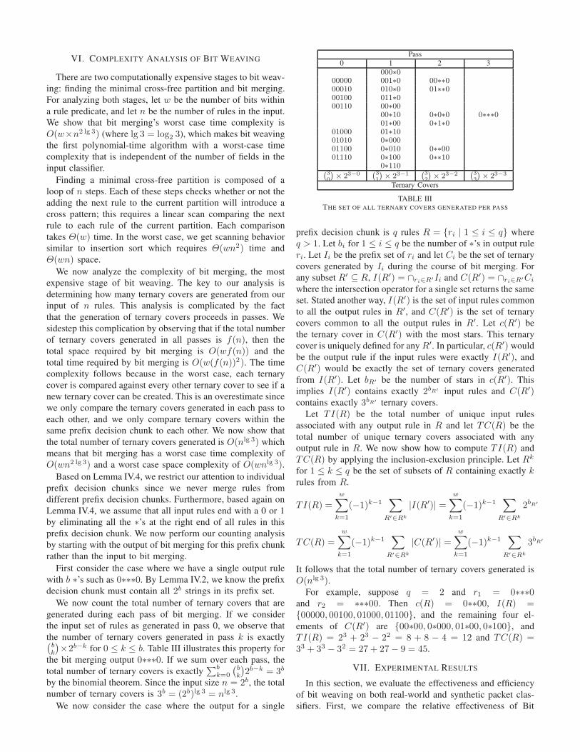
bk

)

×2b−k for 0 ≤ k ≤ b. Table III illustrates this property for

the bit merging output 0∗∗∗0. If we sum over each pass, the

total number of ternary covers is exactly∑b

k=0

(

b

k

)

2b−k = 3b

by the binomial theorem. Since the input size n = 2b, the total

number of ternary covers is 3b = (2b)lg 3 = nlg 3.

We now consider the case where the output for a single

Pass

0 1 2 3

000∗0

00000 001∗0 00∗∗0

00010 010∗0 01∗∗0

00100 011∗0

00110 00∗00

00∗10 0∗0∗0 0∗∗∗0

01∗00 0∗1∗0

01000 01∗10

01010 0∗000

01100 0∗010 0∗∗00

01110 0∗100 0∗∗10

0∗110(30

)

× 23−0

(31

)

× 23−1

(32

)

× 23−2

(33

)

× 23−3

Ternary Covers

TABLE IIITHE SET OF ALL TERNARY COVERS GENERATED PER PASS

prefix decision chunk is q rules R = {ri | 1 ≤ i ≤ q} where

q > 1. Let bi for 1 ≤ i ≤ q be the number of ∗’s in output rule

ri. Let Ii be the prefix set of ri and let Ci be the set of ternary

covers generated by Ii during the course of bit merging. For

any subset R′ ⊆ R, I(R′) = ∩ri∈R′Ii and C(R′) = ∩ri∈R′Ci

where the intersection operator for a single set returns the same

set. Stated another way, I(R′) is the set of input rules common

to all the output rules in R′, and C(R′) is the set of ternary

covers common to all the output rules in R′. Let c(R′) be

the ternary cover in C(R′) with the most stars. This ternary

cover is uniquely defined for any R′. In particular, c(R′) would

be the output rule if the input rules were exactly I(R′), and

C(R′) would be exactly the set of ternary covers generated

from I(R′). Let bR′ be the number of stars in c(R′). This

implies I(R′) contains exactly 2bR′ input rules and C(R′)contains exactly 3bR′ ternary covers.

Let TI(R) be the total number of unique input rules

associated with any output rule in R and let TC(R) be the

total number of unique ternary covers associated with any

output rule in R. We now show how to compute TI(R) and

TC(R) by applying the inclusion-exclusion principle. Let Rk

for 1 ≤ k ≤ q be the set of subsets of R containing exactly k

rules from R.

TI(R) =w∑

k=1

(−1)k−1∑

R′∈Rk

|I(R′)| =w∑

k=1

(−1)k−1∑

R′∈Rk

2bR′

TC(R) =

w∑

k=1

(−1)k−1∑

R′∈Rk

|C(R′)| =w∑

k=1

(−1)k−1∑

R′∈Rk

3bR′

It follows that the total number of ternary covers generated is

O(nlg 3).For example, suppose q = 2 and r1 = 0∗∗∗0

and r2 = ∗∗∗00. Then c(R) = 0∗∗00, I(R) ={00000, 00100, 01000, 01100}, and the remaining four el-

ements of C(R′) are {00∗00, 0∗000, 01∗00, 0∗100}, and

TI(R) = 23 + 23 − 22 = 8 + 8 − 4 = 12 and TC(R) =33 + 33 − 32 = 27 + 27− 9 = 45.

VII. EXPERIMENTAL RESULTS

In this section, we evaluate the effectiveness and efficiency

of bit weaving on both real-world and synthetic packet clas-

sifiers. First, we compare the relative effectiveness of Bit

Weaving (BW) and the state-of-the-art classifier compression

scheme, TCAM Razor (TR) [13]. Then, we evaluate how much

additional compression results from enhancing prior compres-

sion techniques TCAM Razor and Topological Transformation

(TT) [17] with bit weaving.

A. Evaluation Metrics and Data Sets

We first define the following notation. We use C to denote

a classifier, |C| to denote the number of rules in C, S to

denote a set of classifiers, A to denote a classifier minimization

algorithm, A(C) to denote the classifier produced by applying

algorithm A on C, and Direct(C) to denote the classifier

produced by applying direct prefix expansion on C.

We define six basic metrics for assessing the performance

of classifier minimization algorithm A on a set of classifiers

S as shown in Table IV. The improvement ratio of A′ over A

assesses how much additional compression is achieved when

adding A′ to A. A does well when it achieves small com-

pression and expansion ratios and large improvement ratios.

Compression Ratio

Average Total

ΣC∈S

|A(C)||Direct(C)|

|S|ΣC∈S |A(C)|

ΣC∈S |Direct(C)|

Expansion Ratio

Average Total

ΣC∈S

|A(C)||C|

|S|

ΣC∈S |A(C)|

ΣC∈S |C|

Improvement Ratio

Average Total

ΣC∈S

|A(C)|−|A′(C)||A(C)|

|S|

ΣC∈S |A(C)|−|A′(C)|

ΣC∈S |A(C)|

TABLE IVMETRICS FOR A ON A SET OF CLASSIFIERS S

We use RL to denote a set of 25 real-world packet classifiers

that we performed experiments on. The classifiers range in size

from a handful of rules to thousands of rules. We obtained RL

from several network service providers where many classifiers

from the same provider are structurally similar varying only in

the IP prefixes of some rules. When we run any compression

algorithms on these structurally similar classifiers, we get

essentially identical results. We eliminated the resulting double

counting of results that would bias the resulting averages

by randomly choosing a single classifier from each set of

structurally similar classifiers to be in RL. We then split

RL into two groups, RLa and RLb, where the expansion

ratio of direct expansion is less then 2 in RLa and the

expansion ratio of direct expansion is greater than 40 in RLb.

We have no classifiers where the expansion ratio of direct

expansion is between 2 and 40. It turns out |RLa| = 12 and

|RLb| = 13. By separating these classifiers into two groups,

we can determine how well our techniques work on classifiers

that do suffer significantly from range expansion as well as

those that do not.

Due to security concerns, it is difficult to acquire a large

quantity of real-world classifiers. We generated a set of 150synthetic classifiers SY N with the number of rules ranging

from 250 to 8000. The predicate of each rule has five fields:

source IP, destination IP, source port, destination port, and

protocol. We based our generation method upon Singh et al.’s

[30] model of synthetic rules. We also performed experiments

on TRS, a set of 490 classifiers produced by Taylor&Turner’s

Classbench [31]. These classifiers were generated using the

parameters files downloaded from Taylor’s web site (http:

//www.arl.wustl.edu/∼det3/ClassBench/index.htm). To represent a

wide range of classifiers, we chose a uniform sampling of

the allowed values for the parameters of smoothness, address

scope, and application scope.

To stress test the sensitivity of our algorithms to the number

of classifier decisions, we created a set of classifiers RLU (and

thus RLaU and RLbU ) by replacing the decision of every rule

in each classifier by a unique decision. Similarly, we created

the set SY NU . Thus, each classifier in RLU (or SYNU ) has

the maximum possible number of distinct decisions.

B. Effectiveness of Bit Weaving Alone

Table V shows the average and total compression ratios, and

the average and total expansion ratios for TCAM Razor and

Bit Weaving on all nine data sets. Figures 5 and 6 show the

specific compression ratios for all of our real-world classifiers,

and Figures 7 and 8 show the specific expansion ratios for all

of our real-world classifiers. Clearly, bit weaving is an effective

algorithm with an average compression ratio of 23.6% on our

real-world classifiers and 34.6% when these classifiers have

unique decisions. This is very similar to TCAM Razor, the

previous best known-compression method.

One interesting observation is that TCAM Razor and bit

weaving seem to be complementary techniques. That is,

TCAM Razor and bit weaving seem to find and exploit

different compression opportunities. Bit weaving is more

effective on RLa while TCAM Razor is more effective on

RLb. TCAM Razor is more effective on classifiers that suffer

from range expansion because it has more options to mitigate

range expansion including introducing new rules to eliminate

bad ranges. On the other hand, by exploiting non-prefix

optimizations, bit weaving’s ability to find rules that can be

merged is more effective than TCAM Razor on classifiers that

do not experience significant range expansion.

C. Improvement Effectiveness of Bit Weaving

Table V shows the improvement to average and total

compression and expansion ratios when TCAM Razor and

Topological Transformation are enhanced with bit weaving on

all nine data sets. Figures 9 and 10 show how bit weaving

improved compression for each of our real-world classifiers.

Our results for enhancing TCAM Razor with bit weaving

is actually the best result from three different possible com-

positions: bit weaving alone, TCAM Razor followed by bit

weaving, and a TCAM Razor algorithm that uses bit merging

to compress each intermediate classifier generated during the

execution of TCAM Razor as discussed in Section V-C.

Topological Transformation is enhanced by performing bit

merging on each of its encoding tables. We do not perform

bit weaving on the encoded classifier because the nature

of Topological Transformation produces encoded classifiers

that do not benefit from non-prefix encoding. Therefore, for

Topological Transformation, we report only the improvement

to storing the encoding tables.

0 2 4 6 8 10 12Classifier

0

20

40

60

80

100

Com

pre

ssio

n R

ati

o (

Perc

enta

ge) TCAM Razor

Bit Weaving

Fig. 5. Compression ratio for RLa

0 2 4 6 8 10 12 14Classifier

0

1

2

3

4

5

6

7

8

9

Com

pre

ssio

n R

ati

o (

Perc

enta

ge) TCAM Razor

Bit Weaving

Fig. 6. Compression ratio for RLb

0 2 4 6 8 10 12Classifier

0

20

40

60

80

100

120

Expansio

n R

ati

o (

Perc

enta

ge)

TCAM RazorBit Weaving

Fig. 7. Expansion ratio for RLa

0 2 4 6 8 10 12 14Classifier

0

100

200

300

400

500

600

700

Expansio

n R

ati

o (

Perc

enta

ge)

TCAM RazorBit Weaving

Fig. 8. Expansion ratio for RLb

0 2 4 6 8 10 12Classifier

0

10

20

30

40

50

60

Impro

vem

ent

Rati

o (

Perc

enta

ge) TCAM Razor

Topo. Trans.

Fig. 9. Improvement for RLa

0 2 4 6 8 10 12 14Classifier

0

10

20

30

40

50

60

Impro

vem

ent

Rati

o (

Perc

enta

ge) TCAM Razor

Topo. Trans.

Fig. 10. Improvement for RLb

Compression Ratio Expansion Ratio Improvement Ratio

Average Total Average Total Average Total

TR BW TR BW TR BW TR BW TR TT TR TT

RL 24.5 % 23.6 % 8.8 % 10.7 % 59.8 % 222.9 % 30.1 % 36.8 % 12.8 % 36.5 % 12.8 % 38.9 %

RLa 50.1 % 44.0 % 26.7 % 23.7 % 54.6 % 48.0 % 29.0 % 25.7 % 11.9 % 40.4 % 12.7 % 39.9 %

RLb 0.8 % 4.8 % 0.8 % 5.0 % 64.7 % 384.3 % 65.1 % 397.7 % 13.6 % 32.8 % 14.3 % 34.7 %

RLU 31.9 % 34.6 % 13.1 % 17.1 % 146.2 % 465.5 % 45.0 % 58.8 % 3.5 % 35.6 % 2.8 % 38.2 %

RLaU 62.9 % 61.6 % 36.0 % 35.0 % 68.7 % 67.2 % 39.1 % 38.0 % 2.0 % 40.6 % 2.9 % 39.3 %

RLbU 3.3 % 9.6 % 3.0 % 9.2 % 217.7 % 833.1 % 237.6 % 732.6 % 4.8 % 30.9 % 2.1 % 32.7 %

SY N 10.4 % 9.7 % 7.8 % 7.3 % 12.3 % 11.5 % 9.3 % 8.7 % 8.1 % 42.0 % 9.4 % 43.2 %

SY NU 42.7 % 41.2 % 38.4 % 36.2 % 50.8 % 49.0 % 45.8 % 43.2 % 3.9 % 43.3 % 5.7 % 44.1 %

TRS 13.8 % 7.8 % 20.6 % 10.3 % 41.7 % 21.3 % 45.2 % 22.7 % 32.9 % 34.0 % 49.7 % 33.6 %

TABLE VEXPERIMENTAL RESULTS FOR ALL DATA SETS FOR TCAM RAZOR (TR), BIT WEAVING (BW), AND TOPOLOGICAL TRANSFORMATION (TT)

Bit weaving significantly improves both TCAM Razor and

Topological Transformation with an improvement ratio of

12.8% and 38.9%, respectively. TCAM Razor and bit weaving

exploit different compression opportunities so they compose

well. Bit weaving significantly helps Topological Transforma-

tion because each encoding table of Topological Transforma-

tion is essentially the projection of the classifier along the

given field. Thus each encoding table contains every relevant

range in that field. This leads to non-adjacent intervals with

the same decision that can benefit from bit merging.

D. Efficiency

We implemented all algorithms on Microsoft .Net frame-

work 2.0. Our experiments were carried out on a desktop

PC running Windows XP with 8G memory and a single 2.81GHz AMD Athlon 64 X2 5400+. All algorithms used a single

processor core. On RL, the minimum, mean, median, and

maximum running times of our bit weaving algorithm (ex-

cluding the time of running the redundancy removal algorithm

before and after running our bit weaving algorithm) were

0.0002, 0.0339, 0.0218, and 0.1554 seconds, respectively; on

RLU , the minimum, mean, median, and maximum running

times of our bit weaving algorithm were 0.0003, 0.2151,

0.0419, and 1.7842 seconds, respectively. On synthetic rules,

the running time of bit weaving grows linearly with the number

of rules in a classifier, where the average running time for

classifiers of 8000 rules is 0.2003 seconds.

VIII. CONCLUSION

Bit weaving is the first TCAM compression method that

can create non-prefix field classifiers and runs in polynomial

time regardless of the number of fields in each rule. It also

supports fast incremental updates to classifiers, and it can be

deployed on existing classification hardware. Given its speed

and its ability to find different compression opportunities than

existing compression schemes, bit weaving should always be

used, either by itself or as a postprocessing routine, whenever

TCAM classifier compression is needed.

Acknowledgement

This material is based in part upon work supported by the

National Science Foundation under Grant Numbers CNS-

0916044 and CNS-0845513. Any opinions, findings, and con-

clusions or recommendations expressed in this material are

those of the authors and do not necessarily reflect the views

of the National Science Foundation.

REFERENCES

[1] Karthik Lakshminarayanan, Anand Rangarajan, and Srinivasan Venkat-achary, “Algorithms for advanced packet classification with ternaryCAMs”, in Proc. ACM SIGCOMM, August 2005, pp. 193 – 204.

[2] “Integrated Device Technology, Inc. Content addressable memory.http://www.idt.com/”.

[3] David E. Taylor, “Survey & taxonomy of packet classification tech-niques”, ACM Computing Surveys, vol. 37, no. 3, pp. 238–275, 2005.

[4] Banit Agrawal and Timothy Sherwood, “Modeling tcam power fornext generation network devices”, in Proc. IEEE Int. Symposium on

Performance Analysis of Systems and Software, 2006, pp. 120– 129.[5] Cristian Lambiri, “Senior staff architect IDT, private communication”,

2008.[6] Panos C. Lekkas, Network Processors - Architectures, Protocols, and

Platforms, McGraw-Hill, 2003.[7] Fang Yu, T. V. Lakshman, Marti Austin Motoyama, and Randy H. Katz,

“SSA: A power and memory efficient scheme to multi-match packetclassification”, in Proc. Symposium on Architectures for Networking

and Communications Systems (ANCS), October 2005, pp. 105–113.[8] Richard Draves, Christopher King, Srinivasan Venkatachary, and Brian

Zill, “Constructing optimal IP routing tables”, in Proc. IEEE INFO-

COM, 1999, pp. 88–97.[9] Subhash Suri, Tuomas Sandholm, and Priyank Warkhede, “Compressing

two-dimensional routing tables”, Algorithmica, vol. 35, pp. 287–300,2003.

[10] David A. Applegate, Gruia Calinescu, David S. Johnson, HowardKarloff, Katrina Ligett, and Jia Wang, “Compressing rectilinear picturesand minimizing access control lists”, in Proc. ACM-SIAM Symposium

on Discrete Algorithms (SODA), January 2007.

[11] Qunfeng Dong, Suman Banerjee, Jia Wang, Dheeraj Agrawal, andAshutsh Shukla, “Packet classifiers in ternary CAMs can be smaller”,in Proc. ACM Sigmetrics, 2006, pp. 311–322.

[12] Alex X. Liu and Mohamed G. Gouda, “Complete redundancy removalfor packet classifiers in tcams”, IEEE Transactions on Parallel and

Distributed Systems (TPDS), to appear.[13] Alex X. Liu, Chad R. Meiners, and Eric Torng, “TCAM razor: A

systematic approach towards minimizing packet classifiers in TCAMs”,IEEE/ACM Transactions on Networking, vol. 18, no. 2, pp. 490–500,April 2010.

[14] Alex X. Liu and Mohamed G. Gouda, “Complete redundancy detectionin firewalls”, in Proc. 19th Annual IFIP Conf. on Data and ApplicationsSecurity, LNCS 3654, August 2005, pp. 196–209.

[15] Alex X. Liu, Chad R. Meiners, and Yun Zhou, “All-match basedcomplete redundancy removal for packet classifiers in TCAMs”, in Proc.27th Annual IEEE Conf. on Computer Communications (Infocom), April2008.

[16] Rick McGeer and Praveen Yalagandula, “Minimizing rulesets for tcamimplementation”, in Proc. IEEE Infocom, 2009.

[17] Chad R. Meiners, Alex X. Liu, and Eric Torng, “Topological transforma-tion approaches to optimizing tcam-based packet processing systems”,in Proc. ACM SIGCOMM (poster session), August 2008.

[18] Anat Bremler-Barr and Danny Hendler, “Space-efficient TCAM-basedclassification using gray coding”, in Proc. 26th Annual IEEE Conf. on

Computer Communications (Infocom), May 2007.

[19] Huan Liu, “Efficient mapping of range classifier into Ternary-CAM”,in Proc. Hot Interconnects, 2002, pp. 95– 100.

[20] Jan van Lunteren and Ton Engbersen, “Fast and scalable packetclassification”, IEEE Journals on Selected Areas in Communications,vol. 21, no. 4, pp. 560– 571, 2003.

[21] D. Pao, P. Zhou, Bin Liu, and X. Zhang, “Enhanced prefix inclusioncoding filter-encoding algorithm for packet classification with ternarycontent addressable memory”, Computers & Digital Techniques, IET,vol. 1, pp. 572–580, April 2007.

[22] Hao Che, Zhijun Wang, Kai Zheng, and Bin Liu, “DRES: Dynamicrange encoding scheme for tcam coprocessors”, IEEE Transactions on

Computers, vol. 57, no. 7, pp. 902–915, 2008.[23] Anat Bremler-Barr, David Hay, Danny Hendler, and Boris Farber,

“Layered interval codes for TCAM based classification”, in Proc. of

IEEE Infocom, 2009.[24] Ed Spitznagel, David Taylor, and Jonathan Turner, “Packet classification

using extended TCAMs”, in Proc. 11th IEEE Int. Conf. on Network

Protocols (ICNP), November 2003, pp. 120– 131.[25] Kai Zheng, Chengchen Hu, Hongbin Lu, and Bin Liu, “A TCAM-

based distributed parallel ip lookup scheme and performance analysis”,IEEE/ACM Transactions on Networking, vol. 14, no. 4, pp. 863–875,2006.

[26] Kai Zheng, Hao Che, Zhijun Wang, Bin Liu, and Xin Zhang, “DPPC-RE: TCAM-based distributed parallel packet classification with rangeencoding”, IEEE Transactions on Computers, vol. 55, no. 8, pp. 947–961, 2006.

[27] Chad R. Meiners, Alex X. Liu, and Eric Torng, “TCAM Razor: Asystematic approach towards minimizing packet classifiers in TCAMs”,in Proc. 15th IEEE Conf. on Network Protocols (ICNP), October 2007,pp. 266–275.

[28] Richard W. Hamming, “Error detecting and correcting codes”, Bell

Systems Technical Journal, vol. 29, pp. 147–160, April 1950.[29] Chad R. Meiners, Alex X. Liu, and Eric Torng, “Algorithmic approaches

to redesigning tcam-based systems [extended abstract]”, in Proc. ACM

SIGMETRICS, June 2008.[30] Sumeet Singh, Florin Baboescu, George Varghese, and Jia Wang,

“Packet classification using multidimensional cutting”, in Proc. ACMSIGCOMM, 2003, pp. 213–224.

[31] David E. Taylor and Jonathan S. Turner, “Classbench: A packetclassification benchmark”, in Proc. IEEE Infocom, March 2005.

Chad R. Meiners received his Ph.D. in ComputerScience at Michigan State University in 2009. Heis currently technical staff at MIT Lincoln Lab-oratory. His research interests include networking,algorithms, and security.

Alex X. Liu received his Ph.D. degree in computerscience from the University of Texas at Austin in2006. He is currently an assistant professor in theDepartment of Computer Science and Engineeringat Michigan State University. He received the IEEE& IFIP William C. Carter Award in 2004 and anNSF CAREER award in 2009. He received theMSU College of Engineering Withrow DistinguishedScholar Award in 2011. His research interests focuson networking, security, and dependable systems.

Eric Torng received his Ph.D. degree in computerscience from Stanford University in 1994. He is cur-rently an associate professor and graduate directorin the Department of Computer Science and Engi-neering at Michigan State University. He received anNSF CAREER award in 1997. His research interestsinclude algorithms, scheduling, and networking.