6.02 Spring 2011 Lecture 7, Slide #1

6.02 Spring 2011

Lecture #7

•  ISI and BER • Choosing Vth to minimize BER

6.02 Spring 2011 Lecture 7, Slide #2

Bit Error Rate

The bit error rate (BER), or perhaps more appropriately the bit error ratio, is the number of bits received in error divided by the total number of bits transferred. We can estimate the BER by calculating the probability that a bit will be incorrectly received due to noise. Using our normal signaling strategy (0V for “0”, 1V for “1”), on a noise-free channel with no ISI, the samples at the receiver are either 0V or 1V. Assuming that 0’s and 1’s are equally probable in the transmit stream, the number of 0V samples is approximately the same as the number of 1V samples. So the mean and power of the noise-free received signal are

µynf=1N

ynf [n]=n=1

N

! 1NN2=12

!Pynf =1N

ynf [n]"12

#

$%

&

'(2

=n=1

N

! 1N

12#

$%&

'(2

=n=1

N

! 1NN4=14

6.02 Spring 2011 Lecture 7, Slide #3

p(bit error)

Now assume the channel has Gaussian noise with μ=0 and variance σ2. And we’ll assume a digitization threshold of 0.5V. We can calculate the probability that noise[k] is large enough that y[k] = ynf[k] + noise[k] is received incorrectly:

p(error | transmitted “0”):

0

σ

0.5

1-Φμ,σ(0.5) = Φμ,σ(-0.5) = Φ((-0.5-0)/σ) = Φ(-0.5/σ)

p(error | transmitted “1”):

0.5 1

σ

Φμ,σ(0.5) = Φ((0.5-1)/σ) = Φ(-0.5/σ)

p(bit error) = p(transmit “0”)*p(error | transmitted “0”) + p(transmit “1”)*p(error | transmitted “1”)

= 0.5*Φ(-0.5/σ) + 0.5*Φ(-0.5/σ) = Φ(-0.5/σ)

Plots of noise-free voltage + Gaussian noise

6.02 Spring 2011 Lecture 7, Slide #4

BER (no ISI) vs. SNR

SNR (db) =10 log!Psignal!Pnoise

!

"##

$

%&&=10 log 0.25

! 2

!

"#

$

%&

We calculated the power of the noise-free signal to be 0.25 and the power of the Gaussian noise is its variance, so

Given an SNR, we can use the formula above to compute σ2 and then plug that into the formula on the previous slide to compute p(bit error) = BER. The BER result is plotted to the right for various SNR values.

6.02 Spring 2011 Lecture 7, Slide #5

Intersymbol Interference and BER

Consider transmitting a digital signal at 3 samples/bit over a channel whose h[n] is shown on the left below.

The figure on the right shows that at end of transmitting each bit, the voltage y[n] corresponding to the last sample in the bit will have one of 4 values and depends only on the current bit and previous bit.

y[5]=0.0V

y[5]=0.3V

y[5]=0.7V

y[5]=1.0V

6.02 Spring 2011 Lecture 7, Slide #6

Test Sequence to Generate Eye Diagram

If we want to explore every possible transition over the channel, we’ll need to consider transitions that start at each of the four voltages from the previous slide, followed by the transmission of a “0” and a “1”, i.e., all patterns of 3 bits.

6.02 Spring 2011 Lecture 7, Slide #7

The Eight Cases

The first two bits determine the starting voltage, the third bit is the test bit. The plots show the response to the test bit. All bits transmitted at 3 samples/bit.

6.02 Spring 2011 Lecture 7, Slide #8

Plot the Eye Diagram

To make an eye diagram, overlay the eight plots in a single diagram. We can label the plot with the bit sequence that generated each line. The widest part of the eye comes at the first sample in each bit. Using the convolution sum we can compute the width of the eye = 0.8-0.2 = 0.6V

111

011 110

010

101

001 100

000

y[n]=0.2*0 + 0.2*1 + 0.3*1 + 0.3*1 = 0.8V

y[n]=0.2*1 + 0.2*0 + 0.3*0 + 0.3*0 = 0.2V

6.02 Spring 2011 Lecture 7, Slide #9

BER and ISI

From the diagram on the previous slide, if we sample at the widest point in the eye, the noise-free signal will produce one of four possible samples:

1.  1.0V if last two bits are “11” 2.  0.8V if last two bits are “10” 3.  0.2V if last two bits are “01” 4.  0.0V if last two bits are “00”

Since all the sequences are equally likely, the probability of observing a particular voltage is 0.25. Let’s repeat the calculation of p(bit error), this time on a channel with ISI, assuming Gaussian noise with a variance of σ2 (from now on we’ll assume that Gaussian noise has a mean of 0). Again, we’ll use a digitization threshold of 0.5V.

6.02 Spring 2011 Lecture 7, Slide #10

p(bit error) with ISI

p(error | 11) = Φ((0.5-1.0)/σ) = Φ(-0.5/σ)

p(error | 10) = Φ((0.5-0.8)/σ) = Φ(-0.3/σ)

p(error | 01) = 1-Φ((0.5-0.2)/σ) = Φ(-0.3/σ)

p(error | 00) = Φ((0.5-1)/σ) = Φ(-0.5/σ)

6.02 Spring 2011 Lecture 7, Slide #11

p(bit error) with ISI cont’d.

p(bit error) = p(11)*p(error | 11) + p(10)*p(error | 10) +

p(01)*p(error | 01) + p(00)*p(error | 00)

= 0.25*Φ(-0.5/σ) + 0.25*Φ(-0.3/σ) +

0.25*Φ(-0.3/σ) + 0.25*Φ(-0.5/σ)

= 0.5*Φ(-0.5/σ) + 0.5*Φ(-0.3/σ)

Suppose σ=0.25. Compare the formula above to the formula on slide #3 to determine what ISI has cost us in terms of BER: p(bit error, no ISI) = Φ(-0.5/0.25) = Φ(-2) = 0.023 p(bit error, with ISI) = 0.5*Φ(-2) + 0.5*Φ(-1.2) = 0.069 Bottom line: a factor of 3 increase in BER

6.02 Spring 2011 Lecture 7, Slide #12

Choosing Vth

We’ve been using 0.5V as the digitization threshold – it’s the voltage half-way between the two signaling voltages of 0V and 1V. Assuming that the probability of transmitting 0’s and 1’s is the same, this choice minimizes the BER. Let’s see why… Suppose noise has a triangular distribution from -0.6V to 0.6V:

0.5 0 0.6 -0.6

0.417

PDF of received 0’s

1 0.4 1.6

PDF of received 1’s

PDF of received signal

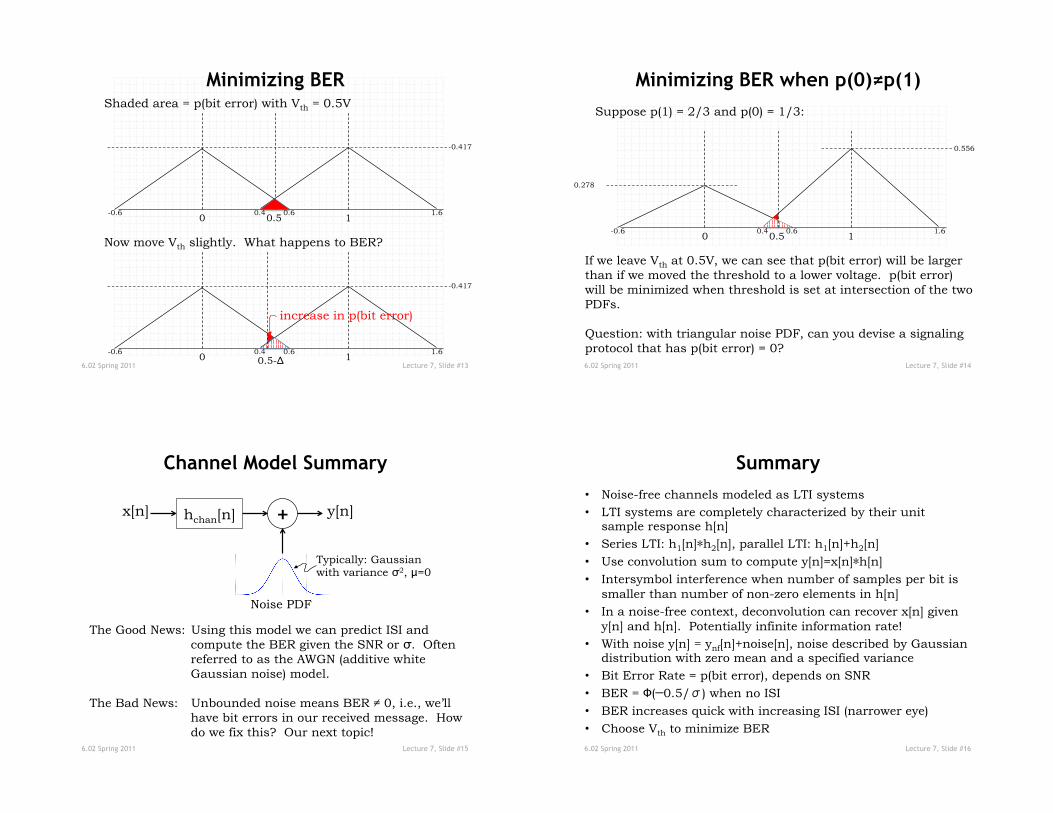
6.02 Spring 2011 Lecture 7, Slide #13

Minimizing BER

0.5 0 0.6 -0.6

0.417

1 0.4 1.6

Shaded area = p(bit error) with Vth = 0.5V

Now move Vth slightly. What happens to BER?

0.5-Δ 0 0.6 -0.6

0.417

1 0.4 1.6

increase in p(bit error)

6.02 Spring 2011 Lecture 7, Slide #14

Minimizing BER when p(0)!p(1)

0.5 0 0.6 -0.6

0.556

1 0.4 1.6

Suppose p(1) = 2/3 and p(0) = 1/3:

If we leave Vth at 0.5V, we can see that p(bit error) will be larger than if we moved the threshold to a lower voltage. p(bit error) will be minimized when threshold is set at intersection of the two PDFs. Question: with triangular noise PDF, can you devise a signaling protocol that has p(bit error) = 0?

0.278

6.02 Spring 2011 Lecture 7, Slide #15

Channel Model Summary

hchan[n] x[n] y[n] +

Noise PDF

Typically: Gaussian with variance σ2, μ=0

The Good News: Using this model we can predict ISI and compute the BER given the SNR or σ. Often referred to as the AWGN (additive white Gaussian noise) model.

The Bad News: Unbounded noise means BER ! 0, i.e., we’ll have bit errors in our received message. How do we fix this? Our next topic!

6.02 Spring 2011 Lecture 7, Slide #16

Summary

•  Noise-free channels modeled as LTI systems

•  LTI systems are completely characterized by their unit sample response h[n]

•  Series LTI: h1[n] h2[n], parallel LTI: h1[n]+h2[n]

•  Use convolution sum to compute y[n]=x[n] h[n]

•  Intersymbol interference when number of samples per bit is smaller than number of non-zero elements in h[n]

•  In a noise-free context, deconvolution can recover x[n] given y[n] and h[n]. Potentially infinite information rate!

•  With noise y[n] = ynf[n]+noise[n], noise described by Gaussian distribution with zero mean and a specified variance

•  Bit Error Rate = p(bit error), depends on SNR

•  BER = Φ(－0.5/σ) when no ISI

•  BER increases quick with increasing ISI (narrower eye)

•  Choose Vth to minimize BER