Bistatic Synthetic Aperture Radar using GNSS as Transmitters of
328
Bistatic Synthetic Aperture Radar using GNSS as Transmitters of Opportunity by RUI ZUO A thesis submitted to The University of Birmingham for the Degree of DOCTOR OF PHILOSOPHY School of Electronic, Electrical and Computer Engineering The University of Birmingham September 2011
Transcript of Bistatic Synthetic Aperture Radar using GNSS as Transmitters of

Bistatic Synthetic Aperture Radar using
GNSS as Transmitters of Opportunity
by
RUI ZUO
A thesis submitted to
The University of Birmingham
for the Degree of
DOCTOR OF PHILOSOPHY
School of Electronic, Electrical
and Computer Engineering
The University of Birmingham
September 2011

University of Birmingham Research Archive
e-theses repository This unpublished thesis/dissertation is copyright of the author and/or third parties. The intellectual property rights of the author or third parties in respect of this work are as defined by The Copyright Designs and Patents Act 1988 or as modified by any successor legislation. Any use made of information contained in this thesis/dissertation must be in accordance with that legislation and must be properly acknowledged. Further distribution or reproduction in any format is prohibited without the permission of the copyright holder.
- i -
Abstract
The thesis summarizes the research on the feasibility investigation of Space-Surface (i.e.
a spaceborne transmitter and an airborne receiver) Bistatic Synthetic Aperture Radar (SS-
BSAR) with a Global Navigation Satellite System (GNSS) which is used as a transmitter
of opportunity. The most promising non-cooperative transmitter, among the existing
GNSS, for the practical radar applications is the newly introduced European Galileo
system. Three main areas are included in the thesis: the system overview, hardware and
experimentation, and the experiential results analysis. The system overview discusses the
key operation principles (topology, synchronization, etc.) of the proposed radar system
and an analysis of the system parameters (power budget, spatial resolution etc.). A
hardware was specially developed and the experiments have been conducted to
investigate the system feasibility and performance. Synchronisation and image formation
algorithms are discussed with the dedication to the proposed radar system. The
experimental results, obtained from the synchronisation, stationary receiver and ground
moving receiver experiments are presented and analysed in the thesis.

- ii -
Acknowledgement
First and foremost I offer my sincerest gratitude to my supervisor, Prof Mike Cherniakov,
who has supported me throughout my thesis writing with his patience and knowledge.
His encouragement, guidance and support from the first day of my PhD to today enabled
me to develop a thorough understanding of the subject.
Secondly, I offer my regards and blessings to all of those who supported me in any
respect during the completion of my PhD project.
Last not the least, I would like to thank my wife and parents for supporting me spiritually
and materially throughout all the years in my life.

- iii -
CONTENTS
Figures v
Tables viii
Abbreviations ix
Chapter 1 Introduction and Background 01
1.1 Radar and Synthetic Aperture Radar 01
1.2 Bistatic Radar 03
1.3 Bistatic Synthetic Aperture Radar 06
1.4 Summary of Research 20
Chapter 2 Non-cooperative Transmitter for SS-BSAR 32
2.1 Introduction 32
2.2 Availability and Reliability 34
2.3 Target Resolution 40
2.4 Power Budget 51
2.5 Summary 68
Chapter 3 GNSS Signals for SS-BSAR Application 71
3.1 Introduction 71
3.2 GNSS Signals Frequency Bands 72
3.3 GNSS Signals Generation and Reception 76
3.4 Correlation Properties 86
3.5 Resolution Enhancement 90
3.6 Summary 95
Chapter 4 Synchronisation using GNSS Signals 97
4.1 Introduction 97
4.2 Signal Acquisition 110
4.3 Signal Tracking 114
4.4 Experimental Verification 129
4.5 Summary 139
Chapter 5 Experimental Hardware 142

- iv -
5.1 Overview 142
5.2 Experimental Hardware Development 143
5.3 Experimental Hardware Testing 160
5.4 Summary 167
Chapter 6 Experimentations and Parameters Estimation 169
6.1 Overview 169
6.2 Stationary Receiver Experiments 172
6.3 Ground Moving Receiver Experiments 170
6.4 Airborne Receiver Experiments 187
6.5 Parameters Estimation 194
6.6 Summary 222
Chapter 7 Experimental Results and Image Analysis 225
7.1 Image Formation Overview 225
7.2 Experimental Image Results – Stationary Receiver 238
7.3 Experimental Image Results – Ground Moving Receiver 251
7.4 Summary 259
Chapter 8 Conclusions and Future Work 261
8.1 Conclusions 261
8.2 Future Work 263
Appendix
A Galileo Spreading Codes Generation 266
B Coordinate and Datum Transformations 269
C Antennas and Front-end 271
D Frequency Synthesizer 283
E Data Acquisition Subsystem 288
F GPS Receiver 301
G Microwave Receiver – Testing Results 302
H Publications List 313

- v -
List of Figures
Figure 1.1: Monostatic SAR Topology (strip-map mode) 2
Figure 1.2: Bistatic Radar in Two Dimensions (courtesy of [6]) 4
Figure 1.3: Bistatic SAR General Topology (spaceborne or airborne platform) 8
Figure 1.4: SS-BSAR, Spaceborne Transmitter and Stationary Receiver 16
Figure 1.5: SS-BSAR, Spaceborne Transmitter and Airborne Receiver 17
Figure 1.6: GNSS based SS-BSAR 21
Figure 1.7: The Block Diagram of the proposed SS-BSAR System 22
Figure 2.1: Bistatic Geometry for SS-BSAR 41
Figure 2.2: Resolution Projection on the Ground Plane 43
Figure 2.3: SS-BSAR Resolution Cell 45
Figure 2.4: Range Resolution Vs Bistatic Angle 47
Figure 2.5: 2D Bistatic Geometry - Local Coordinate 48
Figure 2.6: Bistatic Image Grid: Iso-range Contours and Iso-Doppler Contours 49
Figure 2.7: Bistatic Resolution – Parallel Paths Case 50
Figure 2.8: Bistatic Resolution – Non Parallel Paths Case 51
Figure 2.9: Relationship between Minimum Received Power Level and Elevation Angle
for GLONASS 56
Figure 2.10: the Match Filtering Losses vs. the Heterodyne SNR 61
Figure 2.11: SNR Vs Target Detetion Range 67
Figure 3.1: GNSS Signals Frequency Bands 72
Figure 3.2: Sub-Carrier 77
Figure 3.3: GLONASS Signals Modulation Scheme 79
Figure 3.4: Galileo E5 Modulation Scheme E5 Power Spectrum 81
Figure 3.5: Power Spectrum of AltBOC(15,10) 84
Figure 3.6: PSD for Different Modulations 85
Figure 3.7: ACF of BPSK and Different BOC Modulations 88
Figure 3.8: Mainlobe of Correlation Peak 90
Figure 3.9: Comparison of E5a/b and Full E5 91
Figure 3.10: Shifted and Combined E5 Spectrum 92
Figure 3.11: ACF of Combined E5 Spectrum by Different Shift 93
Figure 3.12: Resolution Ability of E5a/b and Combined E5 with Weighting 94
Figure 4.1: Two Dimension Geometry 103 Figure 4.2: Doppler frequency caused by satellite motion (courtesy of [9]) 105
Figure 4.3: Short Term Variation of Doppler Shift with Elevation for GLONASS 106
Figure 4.4: Synchronisation Algorithm Block Diagram 109

- vi -
Figure 4.5: Acquisition Result for GIOVE-A 112
Figure 4.6: Block Diagram (matched filter) 112
Figure 4.7: Correlation Output of a PRN Code 116
Figure 4.8: PRN Code Wipe-off 119
Figure 4.9: Phase Angle from Two Consecutive Data Sets 124
Figure 4.10: Ambiguous Ranges in Frequency Domain (Courtesy of ) 125
Figure 4.11: Decoding the Navigation Message 128
Figure 4.12: Reference Generation for Range Compression 129
Figure 4.13: Experimental Set-up for Synchronisation Verification 130
Figure 4.14: Photo of Experimental Set-up 130
Figure 4.15: Acquisition Outputs 131
Figure 4.16: Acquisition Outputs for 40 s Data 133
Figure 4.17: Doppler Shift Tracking Outputs 134
Figure 4.18: Phase Tracking Outputs 135
Figure 4.19: Decoded Navigation Message 136
Figure 4.20: Range Compression Results 137
Figure 4.21: FFT of Range Compression Results 138
Figure 5.1: Antennas and RF Front-end 146
Figure 5.2: Experimental Radar Receiver 149
Figure 5.3: Photo of Microwave Receiver 150
Figure 5.4: Microwave Receiver Block Diagram 151
Figure 5.5: Microwave Receiver Receiving Chain (2 channels shown) 153
Figure 5.6: Photo of Data Acquisition Subsystem 158
Figure 5.7: Block Diagram of Data Acquisition Subsystem 159
Figure 5.8: Photo of Other Receiver Subsystems 159
Figure 5.9: Block Diagram of Other Receiver Subsystems 160
Figure 5.10: Heterodyne Channel Antenna Testing Set-up 161
Figure 5.11: Radar Channel Antenna Testing Set-up 162
Figure 5.12: ADC Test Arrangement 163
Figure 5.13: Data Acquisition Subsystem Test Arrangement 164
Figure 5.14: Microwave Receiver Noise Testing 165
Figure 5.15: Microwave Receiver Simplified Testing Arrangement 166
Figure 5.16: Microwave Receiver Full Channel Testing Arrangement 167
Figure 6.1: Experimentation Methodology 169
Figure 6.2: Experimental Set-up for Imaging Data Collection 170
Figure 6.3: Data Collection Geometry for Small Bistatic Angle 173
Figure 6.4: Reflector RCS vs. Receiver-to-target Range 175
Figure 6.5: Hardware Vehicle Installation 176
Figure 6.6: Stationary Receiver – Reference Target 176

- vii -
Figure 6.7: Stationary Imaging – Scene 2 178
Figure 6.8: Ground Moving Receiver Experiment Geometry (Receiver – Target Area)
179
Figure 6.9: Target Detection Range 183
Figure 6.10: Target Area – Short Aperture 184
Figure 6.11: Terrain Profile of Target Area 185
Figure 6.12: Target Area – Long Aperture 186
Figure 6.13: Geometry for Range Swath Calculation 188
Figure 6.14: Geometry for Azimuth Swath Calculation 189
Figure 6.15: Data Collection Geometry for Large Bistatic 190
Figure 6.16: Angle Hardware Helicopter Installation 192
Figure 6.17: Target Area 1 – East Fortune Airfield 193
Figure 6.18: Target Area 2 – PDG Airfield 193
Figure 6.19: Transmitter and Receiver Trajectories with Motion Errors 196
Figure 6.20: Coordinates Extraction for Transmitter and Receiver 202
Figure 6.21: Bistatic Triangle 203
Figure 6.22: Coordinate Localization 209
Figure 6.23: Receiver Parameters Estimation 210
Figure 6.24: Satellite Parameters Estimation 211
Figure 6.25: Baseline Range and Doppler History Estimation 213
Figure 6.26: Comparison between Synchronisation Results and Parameters Estimation
Results 215
Figure 6.27: Motion Compensation (vehicle trial data) 218
Figure 6.28: Motion Compensation (helicopter trial data) 221
Figure 7.1: General BSAR Geometry (2D view) 228
Figure 7.2: Block Diagram for RDA 233
Figure 7.3: Block Diagram of BBPA 235
Figure 7.4: Synchronisation Outputs 239 Figure 7.5: Heterodyne Channel Range Compression Results 242
Figure 7.6: Heterodyne Channel Focusing 243
Figure 7.7: Corner Reflector Imaging Results 245
Figure 7.8: Corner Reflector Imaging Results 247
Figure 7.9: Synchronisation Outputs 248
Figure 7.10: Corner Reflector Imaging Result 2 249
Figure 7.11: Range and Cross Range Cross-sections 250
Figure 7.12: Heterodyne Channel Range Compression Results 250
Figure 7.13: Heterodyne Channel Focusing 252 Figure 7.14: Range Compression of Radar Channel Data 253
Figure 7.15: Range Interpolation Results 254
Figure 7.16: Moving Receiver Imaging Result – GIOVE A 256

- viii -
Figure 7.17: Target Area – Separated Houses 257
Figure 7.18: Moving Receiver Imaging Result – GIOVE B 258
Figure 8.1: Future of GNSS based SS-BSAR 264
Figure A.1: Code Construction Principle 267
Figure A.2: Linear Shift Register based Code Generator 267
Figure C.1: Radiation Pattern of Spiral Helix Antennas 271
Figure C.2: Heterodyne Channel Antenna Concept 272
Figure C.3: Return Loss, S11 273
Figure C.4: Impedance 274
Figure C.5: VSWR 274
Figure C.6: Antenna PCB Layout 275
Figure C.7: Heterodyne Channel Antenna Assembly 275
Figure C.8: Radar Channel Antenna Concept 276
Figure C.9: Heterodyne Channel Antenna Testing Set-up 277
Figure C.10: S-parameter Results 278
Figure C.11: Radar Channel Antenna Testing Set-up 279
Figure C.12: Front-end S-parameters Results 281
Figure D.1: Frequency Synthesizers Output 285
Figure E.1: A/D Converter Circuit Diagram 289
Figure E.2: Data Acquisition Card and Docking Station 291
Figure E.3: Read Scheme of FIFO Mode 293
Figure E.4: Data Acquisition Software Flowchart 295
Figure E.5: Experimental Set-up for DAQ Testing 297
Figure E.6: Data Acquisition Subsystem Testing Results 299
Figure G.1: I/Q Demodulator Distortion Test Diagram 305
Figure G.2: Testing Diagram 306
Figure G.3: Receiver Noise Testing Diagram 306
Figure G.4: Receiver Noise Testing Results 307
Figure G.5: Test Diagram for Receiver with Input Signal 308
Figure G.6: Results for Correlation between Radar and Low-gain Channels 309
Figure G.7: Results for Correlation between Heterodyne and Low-gain Channels 310

- ix -
List of Tables
Table 2-1: Satellite Availability 39
Table 2-2: Potential Range Resolution 46
Table 2-3: Calculation Parameters 47
Table 2-4: Transmitter’s Parameters 53
Table 2-5: Parameters of GNSS Satellite Transmitter 57
Table 2-6: Antenna Size Vs SNR in Heterodyne Channel 62
Table 2-7: Parameters for Power Budget Calculation 64
Table 2-8: Power Budget Calculation 66
Table 3-1: Sidelobe Level of PRN Codes 87
Table 4-1: Doppler Shift Dynamics 107
Table 5-1: Antenna Parameters 146
Table 6-1: Ranging Signal Parameters 171
Table 6-2: Calculation Parameters 174
Table 6-3: Satellite Positions and Reflector Distance 178
Table 6-4: Experiment Parameters 186
Table 6-5: Experiment Parameters 190
Table A-1: Spreading Code Lengths for GIOVE-A and GIOVE-B 266
Table A-2: Primary Code Parameters 268
Table C-1: Spiral Helix Antenna Parameter 271
Table E-1: ADC Module Parts List 289
Table E-2: Sampling Clock Module Parts List 291
Table G-1: Microwave Receiver Parts List 303
Table G-2: AC Coupling Test Results 304
Table G-3: Frequency Synthesizer Test Results 305

- x -
Abbreviations
ACF Auto-Correlation Function
ADC Analog-to-Digital Converter
AF Ambiguity Function
AltBOC Alternative Binary Offset Carrier
ASR Azimuth Sampling Rate
BASS Block Adjustment of Synchronising Signal
BBPA Bistatic Back-Projection Algorithm
BOC Binary Offset Carrier
BPA Back-Projection Algorithm
BPF Band Pass Filter
BPSK Binary Phase Shift Keying
BRCS Bistatic Radar Cross Section
BSAR Bistatic Synthetic Aperture Radar
CCF Cross-correlation Function
CDMA Code Division Multiple Access
CNR Carrier Noise Ratio
CR Corner Reflector
CW Continuous Wave
DFT Discrete Fourier Transform
DLL Delay Lock Loop
DTB-S Digital Television Broadcasting Satellite
ECEF Earth Centered, Earth Fixed
EIRP Effective Isotropic Radiated Power
FDMA Frequency Division Multiple Access
FFT Fast Fourier Transform
FIFO First In First Out
FM Frequency Modulation
FPGA Field Programmable Gate Array
FT Fourier Transform
GEO Geostationary Earth Orbit
GIOVE A/B Galileo In-Orbit Validation Element A/B
GLONASS Global Orbiting Navigation Satellite System
GNSS Global Navigation Satellite System
GPS Global Positioning System
HC Heterodyne Channel

- xi -
HEO High Earth Orbit
HPBW Half-Power Beam Width
ICO Intermediate Circular Orbit
IF Intermediate Frequency
IFFT Inverse Fast Fourier Transform
IFT Inverse Fourier Transform
INS Inertial Navigation System
I/Q In-phase/Quadrature
LEO Low Earth Orbit
LFM Linear Frequency Modulation
LHCP Left Hand Circular Polarisation
LMS Least Mean Square
LNA Low Noise Amplifier
LO Local Oscillator
LOS Line Of Sight
LPF Low Pass Filter
LS Least Square
MEO Medium Earth Orbit
MISL Microwave Integrated Systems Laboratory
NCT Non-Cooperative Transmitter
NRZ Not Return Zero
PCI Peripheral Component Interconnect
PCS Personal Communication Satellite
PLL Phase Lock Loop
PPP Precision Position Processing
PRF Pulse Repetition Frequency
PRN Pseudo-Random Noise
PSF Point Spread Function
PSD Power Spectrum Density
QPSK Quadrature Phase Shift Keying
RCM Range Cell Migration
RC Radar Channel
RCS Radar Cross Section
RDA Range-Doppler Algorithm
RF Radio Frequency
RHCP Right Hand Circular Polarisation
RINEX Receiver Independent Exchange Format
RMS Root Mean Square
RS Reflected Signal

- xii -
SAR Synthetic Aperture Radar
SAW Surface Acoustic Wave
SC Spare Channel
SIR Signal-to-Interference Ratio
SL Synchronization Link
SNIR Signal to Noise and Interference Ratio
SNR Signal-to-Noise Ratio
SS Space-borne Segment
SS-BSAR Space Surface Bistatic Synthetic Aperture Radar
SV Space Vehicle
TLE Two Line Element
UAV Unmanned Aerial Vehicles
VCO Voltage Control Oscillator
VSWR Voltage Standing Wave Ratio
WGS 84 World Geodetic System 1984

Chapter 1 Introduction and Background
- 1 -
Chapter 1 Introduction and Background
1.1 Radar and Synthetic Aperture Radar
The basic concept of radar, which is the detection and location of reflecting objects, was
first demonstrated through the experiments conducted by the German physicist between
1885 and 1888. Following this other evidence on the radar method appeared and was
examined by scientists from many other countries, for example Britain and the USA.
This method did not become truly useful until the transmitter and receiver were
collocated at a single site and pulse waveforms were used. From the 1930s to World War
II, radar was rediscovered and many radar systems were developed almost
simultaneously and independently in many countries [1]. The original systems measured
the range to a target via time delay, and the direction of a target via antenna directivity. It
was not long before Doppler shifts were used to measure target speed. Then, in 1951, it
was discovered that the Doppler shifts could be processed to obtain fine resolution in a
direction that was perpendicular to the range or beam direction. This method was termed
Synthetic Aperture Radar (SAR), which referred to the concept of achieving high
resolution in the cross-range dimension by taking advantage of the motion of the platform
carrying the radar to synthesize the effect of a large antenna aperture through signal
processing [2].
In the remote sensing context, a SAR system makes an image of the Earth’s surface from
a spaceborne or airborne platform. It (Figure 1.1) does this by pointing a radar beam
approximately perpendicular to the sensor’s motion vector, transmitting phase-encoded

Chapter 1 Introduction and Background
- 2 -
pulses, and recording the radar echoes as they reflect off the Earth’s surface. To form an
image, intensity measurements must be taken in two orthogonal directions. One
dimension is parallel to the radar beam, as the time delay of the received echo is
proportional to the distance or range along the beam to the target. The second dimension
of the image is given by the travel of the sensor itself. By integrating the received echo
along the moving platform, the targets along the azimuth direction can be separated by a
fine resolution.
Radar
Moving platform
Antenna beam
footprint
Image scene
Ground track
azimuth
range
Figure 1.1: Monostatic SAR Topology (strip-map mode)

Chapter 1 Introduction and Background
- 3 -
An account of the early development of SAR is given in the first few chapters of [3]. The
imaging of the Earth’s surface by SAR to provide a map-like display can be applied to
military reconnaissance, surveillance and targeting, environmental monitoring, and other
remote sensing applications [1]. The application fields of SAR data are very wide. A
current review of the application of SAR in remote sensing is given in the Manual of
Remote Sensing [4], as well as many websites. The applications include oceanography
(wave spectra, wind speed, velocity of ocean currents), glaciology (snow wetness, snow
water equivalent, glacier monitoring), agriculture (crop classification and monitoring, soil
moisture), geology (terrain discrimination, subsurface imaging), forestry (forest height,
biomass, deforestation), deformation monitoring (volcano, Earthquake and subsidence
monitoring with differential interferometry), environment monitoring (oil spills, flooding,
urban growth, global change), cartography and infrastructure planning as well as military
surveillance and reconnaissance [5]. These applications increase almost daily as new
technologies and innovative ideas are developed.
1.2 Bistatic Radar
Bistatic radar is defined as radar that uses antennas at different locations for transmission
and reception. A transmitting antenna is placed at one site and a receiving antenna is
placed at a second site. They are separated by a distance L called the baseline (see Figure
1.2). The target is located at a third site. Any of the sites can be on the Earth, airborne,
or in space, and may be stationary or moving with respect to the Earth [6]. Surprisingly,
in contrast to most of the currently deployed systems which are working in the
monostatic mode, all early radar experiments were of the bistatic type. Before and during

Chapter 1 Introduction and Background
- 4 -
World War II, Germany, Japan, France and the Soviet Union all deployed bistatic radars
for aircraft detection. Even the famous British Chain Home monostatic radars had a
reversionary bistatic mode. After this bistatic radars went through a few periodic
resurgences in interest when specific bistatic applications were found to be attractive [7].
N
β/2
Tgt
L
N
Baseline
RRRT
RxTx
θT θR
β = θT - θR
Figure 1.2: Bistatic Radar in Two Dimensions (courtesy of [6])
One of the peculiarities of bistatic radar is that the location of the receiver is not revealed
by radar emissions; therefore it has been extensively adopted for defence applications. In
addition, current stealth technology is effective against a monostatic illuminator, whereas
the echoes reflected in other directions cannot be easily reduced. Referring to remote
sensing applications, bistatic data provides additional qualitative and quantitative
measurements of microwave scattering from a surface and the objects on it. In a number

Chapter 1 Introduction and Background
- 5 -
of situations it is possible to combine monostatic and bistatic data reflected from an
observation area and to improve the remote sensing performance.
Passive Bistatic Radar
In recent years there has been growing interest in bistatic radar using transmitters of
opportunity, which is termed passive bistatic radar (PBR) [8]. As there is no need for a
dedicated transmitter, this makes PBR inherently low cost and hence attractive for a
broad range of applications. This technology can utilise existing terrestrial and
spaceborne illuminators, such as narrowband digital audio/TV signals [9, 10], wideband
FM signal [11], spaceborne/mobile communication signals [12-14] and global navigation
signals, etc. There is a relatively wide diffusion of such non-cooperative signal sources.
These sources are stable and their characteristics are well known. This makes their use
reliable and inexpensive. However, it is worth noting that in this case the geometric and
radiometric characteristics of bistatic observation are strictly dictated by illuminator
configuration and operation.
Global navigation satellite systems (GNSS) have a number of advantages over these
restrictions as non-cooperative transmitters (NCT), compared to other signal sources.
Bistatic GNSS radar data can be analysed either by examining the correlation of a
reflected waveform or by using the bistatic synthetic aperture radar (BSAR) theory. The
shape and strength of the reflected correlation waveform is determined by the roughness
and dielectric properties of the surface, while the delay of the reflection with respect to
the direct signal gives information about the distance to the receiver. The possibility of

Chapter 1 Introduction and Background
- 6 -
using these properties for remote sensing with GNSS bistatic radar was first presented in
[15] as a possible means of measuring differences in ocean heights from a satellite. Other
applications include the remote sensing of ocean wave height and wind speeds close to
the ocean surface [16-18] and measurements of soil moisture content [19]. The concept
of bistatic SAR using a non-cooperative transmitter (NCT) can be used to get a more
comprehensive picture of the observed surface. This will be discussed in more detail in
the next section.
1.3 Bistatic Synthetic Aperture Radar
As in bistatic radar generally, a bistatic SAR employs a receiving antenna which is
located separately from the transmitting antenna, and a synthetic aperture is formed by
the motion of one or both antennas (see Figure 1.3). Transmitter and receiver movement
may be independent, the trajectories and velocities may be different and even possibly
uncoordinated. So the signal synchronisation and trajectory control aspects are even
more demanding for bistatic synthetic aperture radar (BSAR), due to the need to form the
synthetic aperture. The first documented experiment of synthetic aperture radar in
bistatic geometry was conducted using ship-borne radar to observe wave conditions [20];
the motion of the ship was used to synthesize apertures approximately 350m long. The
first successful experiment that adopted two airborne SARs flying with programmed
separations showed particular aspects of bistatic scattering from rural and urban areas
[21].

Chapter 1 Introduction and Background
- 7 -
Advantages connected to the use of synthetic apertures (for example in terms of
resolution and image quality parameters) are well known and, consequently, a worldwide
interest in the development and exploitation of BSAR is increasing in the scientific
community and among remote sensing users [22-24]. More recently, a number of bistatic
SAR campaigns have been undertaken by research institutes in Europe. For example, in
2002, QinetiQ performed trials with the two UK systems ESR (transmitter) and ADAS
(receiver) that were installed onboard an aircraft and a helicopter, respectively [25]. In
2003, a joint French-German campaign was carried out with RAMSES from ONERA in
France and E-SAR from DLR in Germany, both of which were installed onboard aircraft
platforms [26]. Also, in 2003 FGAN in Germany collected bistatic SAR data with their
two SAR systems AER-II (transmitter) and PAMIR (receiver) in separate aircrafts [27].
With the launch of the satellite TerraSAR-X, both DLR and FGAN have performed
bistatic SAR experiments using the Spaceborne sensor as a transmitter of opportunity
with FSAR and PAMIR in receive mode, respectively [28, 29].
Although the basic operation of all BSAR systems is much the same, the differences are
mainly a consequence of the geometry employed. As a result, both the general and
specific analytical BSAR research could be directly, or with some modification, applied
to other BSAR systems. Hence, an extensive literature review of past BSAR systems and
current development should highlight the direction of the research carried out by this
thesis. The review would mainly concentrate on the references which report BSAR
system analysis, experimentation descriptions, results and applications, rather than the

Chapter 1 Introduction and Background
- 8 -
references discussing BSAR image formation algorithms, as its derivation and
development is beyond the scope of this study.
Tx
Rx
RR
RT
β
Baseline
Image scene
Moving path
Moving
path
Figure 1.3: Bistatic SAR General Topology (spaceborne or airborne platform)
In the section below, three BSAR classes are considered according to their topologies:
spaceborne, airborne and space-surface systems. From their names one can easily
recognise that in the first case transmitters and receivers are based on two or more
satellites, whereas for airborne systems transmitters and receivers are situated on separate
airborne platforms. The space-surface BSAR (SS-BSAR) consists of a spaceborne
transmitter and a receiver mounted near or on the Earth’s surface. The receivers could be
airborne, mounted on a ground vehicle or onboard a ship, or even at a stationary position
on the ground. For the latter case satellite motion should be used to provide aperture
synthesis.

Chapter 1 Introduction and Background
- 9 -
1.3.1 Spaceborne BSAR
As indicated above, spaceborne BSAR consists of two or more satellites, which could be
located on different orbits; one conventional monostatic SAR transmitter with one or
multiple passive receivers, or vice versa. The reference [30] gives an overview of
innovative technologies and applications for future spaceborne bi- and multi-static SAR
systems. Several operational advantages which will increase the capability, reliability
and flexibility of future SAR missions have been summarized as follows: single-pass
interferometry and sparse aperture sensing; frequent monitoring and increased coverage;
multi-angle observation and flexible geometry; and cost reduction. Challenges have also
been identified, such as precise phase synchronisation, accurate knowledge of orbit
trajectory and multi-static image formation algorithms.
For example, a BSAR system, which combines a geostationary transmitter with multiple
passive receivers in low Earth orbit (LEO) has been proposed and studied by the authors
of [31-33]. A closer look at the resolution cell of such bistatic SAR is included and the
system sensitivity is presented by the calculation of the noise equivalent sigma zero
(NESZ). It concluded that bistatic SAR focusing will be possible on the basis of
appropriately selected ultra-stable quartz oscillators and phase synchronisation will be
required. It also indicated achievable baseline estimation accuracy in the millimetre
range on the basis of a differential evaluation of the GPS carrier phase.
The authors of [34] present a scientific space mission, BISSAT, Bistatic SAR Satellite,
consisting of a satellite carrying a receiving only SAR which receives the signal

Chapter 1 Introduction and Background
- 10 -
transmitted by the existing SAR satellite. According to [35, 36], the BISSAT experiment
would be the first bistatic SAR implementation in space with two separate platforms.
COSMO/SkyMed SAR has been selected as the primary radar. Its constellation consists
of four satellites in one orbital plane. The technical feasibility of the mission has been
demonstrated through the orbit and antenna pointing design for bistatic acquisition. An
analysis of the attainable performance of a bistatic SAR for oceanographic applications,
such as the determination of sea state parameters and the reconstruction of the sea wave
spectrum is reported in [37].
There is another BSAR constellation, TanDEM-X, proposed by German scientists [38],
which is built by adding a second spacecraft to TerraSAR-X and flying two satellites in a
closely controlled formation. Using two spacecraft provides the highly flexible and
reconfigurable imaging geometry required for the different mission objectives. It is the
first demonstration of a bistatic interferometric satellite formation in space, as well as the
first close formation flight in operational mode according to [39, 40]. Several new SAR
techniques will also be demonstrated for the first time such as digital beam forming with
two satellites, single-pass polarimetric SAR interferometry, as well as single-pass along-
track interferometry with varying baselines.
Besides the above-mentioned spaceborne constellation dedicatedly developed for BSAR
applications, a synthetic aperture radar is considered in [41], located on a geosynchronous
receiver, and illuminated by the backscattered energy of satellite broadcast digital audio
or television signals. Spatial resolution, link budget, and possible focusing techniques are

Chapter 1 Introduction and Background
- 11 -
evaluated for the proposed geometry. The main restriction is that only objects that
remain stationary half a day could be imaged by the proposed system. Sea, foliage
screens, and, in general, whatever moves in a few milliseconds would almost certainly
not be imaged. Limited areas could be observed from grounded platforms as well, if it is
the transmitter that wanders in the sky. In this case, the more favourable link budget
allows shorter integration times and therefore the use of LEO communication satellites.
1.3.2 Airborne BSAR
The first results of an airborne bistatic SAR demonstration were published in 1984 by
Auterman [21]. In his experiments both aircraft were constrained to flying parallel flight
paths. But technical problems – like the synchronisation of the oscillators, the involved
adjustment of transmit pulse versus receive gate timing, antenna pointing, flight
coordination, double trajectory measurement and motion compensation and the focusing
of bistatic radar data are still not sufficiently solved. In recent decades, more practical
work on this topic has been reported with successful results [25, 27, 42-51].
Horne and Yates [25] has provided an overview of a programme of research addressing
the problems of airborne bistatic SAR imaging. It has shown that imaging is possible
over a surprising range of bistatic geometries with reasonable efficiency. The theory of
bistatic synchronisation has been set out and the effect of oscillator phase noise
considered in detail, showing that cesium atomic clocks provide a viable solution. The
following work presented in [42] focuses on a fully airborne, synchronised bistatic SAR
demonstration using QinetiQ’s enhanced surveillance radar and the Thales/QinetiQ

Chapter 1 Introduction and Background
- 12 -
airborne data acquisition system, which took place in September 2002. Some of the
bistatic imagery from the trial is presented here and compared and contrasted with the
monostatic imagery collected at the same time. This initial work has shown that, at a
high level, the images appear to be similar to the monostatic ones.
The references [27, 43, 44] deal with an airborne bistatic experiment performed in
November 2003: Two SAR systems of FGAN were flown on two different airplanes, the
AER-II system was used as a transmitter and the PAMIR system as a receiver. Different
spatially invariant flight geometries were tested. High resolution bistatic SAR images
were generated successfully. The bistatic range-Doppler processor and the bistatic back
projection processor were applied to real data. The experiments consisted of several
flight configurations with bistatic angles from 13o up to 76
o.
Similar airborne campaigns are described [45, 46] for the first successes in obtaining
bistatic cross-platform interferograms from a two aircraft SAR acquisition campaign
performed between October 2002 and February 2003 by the DLR and ONERA using
their E-SAR and RAMSES facilities. The main challenging issues in the signal
processing involved are the estimation and compensation of phase drift between the two
radars’ master oscillators (the bistatic receive signal is demodulated with a local oscillator
which is not coherent with the transmitter one) and the determination of the relative
aircraft trajectories - i.e. interferometric baseline – accurate to the millimetre. The two
main geometrical configurations were flown, the quasi-monostatic mode, and a mode
with a large bistatic angle. The authors describe this research programme, including the
Chapter 1 Introduction and Background
- 13 -
preparation phase, the analysis of the technological challenges that had to be solved
before the acquisition, the strategy adopted for bistatic image processing, the first results
and a preliminary analysis of the acquired images.
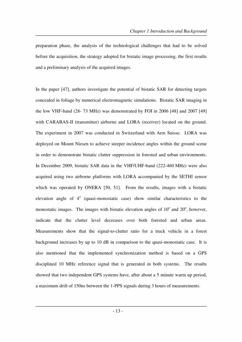
In the paper [47], authors investigate the potential of bistatic SAR for detecting targets
concealed in foliage by numerical electromagnetic simulations. Bistatic SAR imaging in
the low VHF-band (28- 73 MHz) was demonstrated by FOI in 2006 [48] and 2007 [49]
with CARABAS-II (transmitter) airborne and LORA (receiver) located on the ground.
The experiment in 2007 was conducted in Switzerland with Arm Suisse. LORA was
deployed on Mount Niesen to achieve steeper incidence angles within the ground scene
in order to demonstrate bistatic clutter suppression in forested and urban environments.
In December 2009, bistatic SAR data in the VHF/UHF-band (222-460 MHz) were also
acquired using two airborne platforms with LORA accompanied by the SETHI sensor
which was operated by ONERA [50, 51]. From the results, images with a bistatic
elevation angle of 4o (quasi-monostatic case) show similar characteristics to the
monostatic images. The images with bistatic elevation angles of 10o and 20
o, however,
indicate that the clutter level decreases over both forested and urban areas.
Measurements show that the signal-to-clutter ratio for a truck vehicle in a forest
background increases by up to 10 dB in comparison to the quasi-monostatic case. It is
also mentioned that the implemented synchronization method is based on a GPS
disciplined 10 MHz reference signal that is generated in both systems. The results
showed that two independent GPS systems have, after about a 5 minute warm up period,
a maximum drift of 150ns between the 1-PPS signals during 3 hours of measurements.

Chapter 1 Introduction and Background
- 14 -
1.3.3 SS-BSAR
From the SS-BSAR definition, it could have two different configurations, an
airborne/ground moving receiver (Figure 1.5) or a stationary receiver (Figure 1.4). The
distinguishing feature of such systems is their essentially asymmetric topology, the
illumination path being much longer than the echo propagation path. An early SS-BSAR
experiment was conducted in 1994 with the NASA/JPL AIRSAR system acting as the
passive receiver and a spaceborne C-band SAR acting as the illuminator. A range-
Doppler algorithm was used to generate bistatic SAR images [52].
Spaceborne TX – Stationary RX
Most of the BSAR systems proposed in this category are utilising a transmitter of
opportunity, such as broadcasting, communications and navigation satellites, or even a
non-cooperative radar satellite. For example, Griffiths [13] presented a system concept
of a bistatic radar using a satellite-based illuminator of opportunity and a static ground-
based receiver. The properties of the satellite illuminator sources have been reviewed in
terms of coverage, power density and form of signal, leading to the selection of an
Envisat transmitter in low Earth orbit, though it has the significant disadvantage that it is
only available for about one second per orbit repeat.The authors of [53, 54] present the
results of an experimental test which aimed to evaluate the performance of a SAR system
based on the use of an almost geostationary TV satellite as a transmitter and a ground
based receiver. The synthetic aperture can be obtained directly by exploiting the satellite
daily motion. The receiver implemented for the experiment is described. The resolution
capabilities and the link budget of the system have been analysed. It was experimentally

Chapter 1 Introduction and Background
- 15 -
shown that the daily orbit of geostationary TV satellites offers a sufficient synthetic
aperture for realizing a parasitic SAR system with a resolution in azimuth direction of
about 10 m. Authors were able to measure the satellite location and to image an area of
about 40000 m2 (200 m x 200 m), with a ground resolution cell of about 10 x 10 m
2.
X
Z
-Y
Ground
Plane
Satellite
Transmitter
Stationary
ReceiverRR
RT
VT
Target
Area
Figure 1.4: SS-BSAR, Spaceborne Transmitter and Stationary Receiver
According to [55], communication LEOS, such as Globalstar, ICO and Iridium, could
also be effectively used for bistatic synthetic aperture radar design. These satellites
transmit signals in the L or S frequency bands and provide sufficient power spectral
density near the Earth’s surface for effective communication, Moreover, the targets will
be characterised by their bistatic radar cross-section (RCS) that could be 20 to 40 dB
larger than the monostatic RCS [56]. Furthermore, greater improvements in spatial

Chapter 1 Introduction and Background
- 16 -
resolution and/or reduction in spatial ambiguities are achievable by employing a multi-
beam receiver and by simultaneous sensing by multiple LEOS satellites. The direct
communication line could be used for the heterodyne synchronization. The 2-D
resolving capability of such systems is characterized quantitatively within the ground
plane and demonstrated via a meaningful simulation.
Spaceborne TX –Airborne RX
Figure 1.5: SS-BSAR, Spaceborne Transmitter and Airborne Receiver
These papers [29, 57, 58] present the first considerations with respect to the optimization
of possible geometries between the spaceborne and the airborne SAR sensor. It is
concluded that the bistatic geometry has to be adapted to the scene to be imaged. One
has to find a compromise between shading effects, a high resolution, possible restriction

Chapter 1 Introduction and Background
- 17 -
in airspace and the demand to receive the direct satellite signal with the airborne platform.
Due to the extreme platform velocity differences, SAR modes with flexible steering of
the antenna beams are necessary [59]. Several aspects like the ground resolution,
Doppler frequency and Doppler-bandwidth have been analysed. Synchronization
problems, which arise in bistatic SAR missions have been discussed and solutions for the
hybrid bistatic experiment have been presented [60]. Bistatic data acquisition using
TerraSAR-X as a transmitter and PAMIR as a receiver and the image results of two
experiments have been presented and analysed [61]. The data could be focused using a
time-domain and a frequency-domain processor. Finally, the bistatic images have been
compared with the monostatic SAR images of TerraSAR-X and PAMIR.
A special configuration is given [62, 63] when the receive antenna looks in a forward
direction, which is called bistatic forward-looking SAR. These papers analyse a bistatic
forward-looking configuration and demonstrate the capability and feasibility of imaging
in the forward or backward directions using the radar satellite TerraSAR-X as the
transmitter and the airborne SAR system PAMIR as the receiver. The corresponding iso-
range and iso-Doppler contours have been explained. The processed SAR image shows
the feasibility of imaging in the forward direction for the first time using a spatially
separated transmitter and receiver.
Another spaceborne/airborne bistatic experiment was successfully performed early in
November 2007 [64, 65]. TerraSAR-X was used as the transmitter and DLR’s new
airborne radar system, F-SAR, as the receiver. Monostatic data were also recorded during

Chapter 1 Introduction and Background
- 18 -
the acquisition. Since neither absolute range nor Doppler references are available in the
bistatic data set, synchronisation is done with the help of calibration targets on the ground
and based on the analysis of the acquired data compared to expected data.
After the first experiment, DLR performed a second bistatic experiment in July 2008 [66]
with new challenging acquisitions. The new SAR imaging algorithm, based on the fast
factorized back projection algorithm, has demonstrated very good focusing qualities
while dramatically reducing (up to a factor of 100 with respect to direct back projection)
the overall computational load. These papers [67-69] have given a comprehensive report
of the TerraSAR-X/F-SAR bistatic SAR experiment including a description, performance
estimation, data processing and results. The experiment was the first X-band bistatic
spaceborne/airborne acquisition and the first including full synchronization (performed in
processing steps) and high-resolution imaging. The performance analysis presented for
this azimuth-variant acquisition has been validated, including the quantitative analysis of
the effects of antenna patterns on the along-track resolution and SNR. Finally, a
comparison of the monostatic TerraSAR-X and bistatic TerraSAR-X/F-SAR images has
shown some interesting properties. The bistatic image has an advantage in terms of
resolution and SNR and in the complete absence of range ambiguities (highly dependent
on configuration and acquisition).
Besides conventional radar satellites, global navigation satellites are also considered to be
suitable for SS-BSAR applications. For example, in paper [70], the traditional bistatic
GNSS radar and bistatic synthetic aperture radar (SAR) concepts are fused into a more

Chapter 1 Introduction and Background
- 19 -
generic multistatic GNSS SAR system for surface characterization. This is done by using
the range and Doppler processing techniques on signals transmitted by multiple satellites
to determine the angular dependence of the surface reflectivity.
This thesis is dedicated to the case of SS-BSAR with a GNSS transmitter of opportunity
i.e. GPS (US), GLONASS (RU) and Galileo (EU). As the non-cooperative transmitter,
GNSS satellites have advantages and drawbacks in comparison with other signal sources.
The unique feature is that GNSS operates with a large constellation of satellites.
Typically, at any point on the Earth’s surface, 4 to 8 satellites are above the horizon
(Figure 1.6). As a result, a particular satellite in the best (or at least a suitable) position
can be selected and there is no need for a very specific receiver trajectory to allow the
observation of an area. Moreover, signals from more than one satellite could potentially
be used to provide radiogrammetric 3-D surface mapping. Another advantage is a
relatively simple synchronisation of GNSS signals. This follows on from the fact that
navigation signals were designed to be optimal for remote synchronisation.
The main drawback is a relatively low power budget, e.g. Direct Satellite TV (DTB-S)
broadcasting transmitters introduce about a 20 dB stronger power flux density near the
Earth’s surface in comparison to GNSS. The power budget analysis of GNSS based
BSAR is analysed against thermal noise, as well as interference from other satellites [71,
72]. GNSS radiating power is about a 10-15 dB signal-to-noise ratio (SNR) over one
millisecond of integration time at the matched receiver output. The second problem, the
signal-to-interference ratio (SIR), should be evaluated. The direct path interference and

Chapter 1 Introduction and Background
- 20 -
adjacent path interference power density in the targets-receiver areas are near equal
(GNSS transmitting antenna introduce a flat power density near the surface irrelevant to
the satellites elevation up to 10 degrees). Increasing the integration time will result in the
adjacent path interference level decreasing proportionally.
Figure 1.6: GNSS based SS-BSAR
1.4 Summary of Research
1.4.1 Research Contributions
This research focuses on SS-BSAR using GNSS as the transmitter of opportunity. The
main goal of this research is to investigate the feasibility of BSAR systems using
spaceborne navigation satellites and to verify its performance, such as spatial resolution
Chapter 1 Introduction and Background
- 21 -
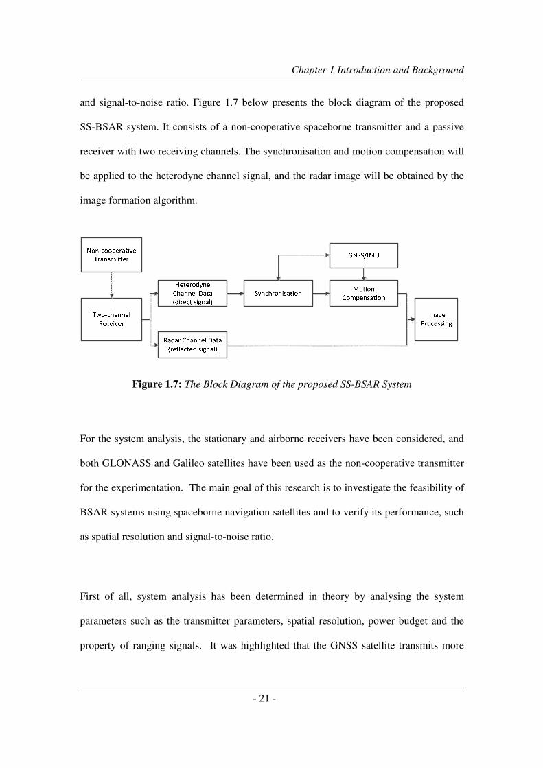
and signal-to-noise ratio. Figure 1.7 below presents the block diagram of the proposed
SS-BSAR system. It consists of a non-cooperative spaceborne transmitter and a passive
receiver with two receiving channels. The synchronisation and motion compensation will
be applied to the heterodyne channel signal, and the radar image will be obtained by the
image formation algorithm.
Figure 1.7: The Block Diagram of the proposed SS-BSAR System
For the system analysis, the stationary and airborne receivers have been considered, and
both GLONASS and Galileo satellites have been used as the non-cooperative transmitter
for the experimentation. The main goal of this research is to investigate the feasibility of
BSAR systems using spaceborne navigation satellites and to verify its performance, such
as spatial resolution and signal-to-noise ratio.
First of all, system analysis has been determined in theory by analysing the system
parameters such as the transmitter parameters, spatial resolution, power budget and the
property of ranging signals. It was highlighted that the GNSS satellite transmits more

Chapter 1 Introduction and Background
- 22 -
than 10 dB less power compared to other satellites. However, it has the advantage of
satellite diversity and thus one can choose the desired bistatic topology for low resolution
loss. It is concluded that overall GNSS satellites are the most suitable non-cooperative
transmitter candidates for SS-BSAR applications. It provides a reasonable range
resolution of ~ 3-8 m and a target detection range of ~ 3-12 km for 50 m2 targets.
As GNSS signals are designed for navigation purposes, one navigation signal (Galileo E5)
has been studied analytically in terms of radar application. Its correlation property has
been investigated by simulation and a technique has been invented to combine full E5
bandwidth and to improve potential range resolution for GNSS based SS-BSAR systems.
Synchronisation, as an inevitable issue for non-cooperative bistatic system, has also been
investigated. In our case, phase synchronisation is the most important, as the largely
separated transmitter and receiver must be coherent over extremely long intervals of time.
Synchronisation using a direct link signal has been proposed and the algorithm to extract
the required information has been applied to the simulated and experimental data.
To obtain the experimental data for image formation and to confirm the system analysis
results, an experimental test bed for the proposed SS-BSAR system has been developed
and tested with full functionality. Experimentation methodology has been planned and a
number of experiments have been conducted. It includes a synchronisation experiment, a
stationary receiver experiment, and a ground moving receiver experiment, and for the
final stage, an airborne receiver experiment. The synchronisation experiment will be
used to prove the functioning of the hardware and the synchronisation algorithm. With

Chapter 1 Introduction and Background
- 23 -
the complexity of the bistatic SAR image formation, a stationary receiver experiment will
be used to test the basic functioning and procedure of the image formation algorithm.
Only after this, the moving receiver experiment can be conducted and a set of data has
been collected according to the above mentioned requirements.
Image formation algorithms for SS-BSAR, such as range-Doppler and back-projection
algorithms have been studied and briefly discussed. As the development of focusing
techniques for general bistatic topology is beyond the scope of this thesis, the detailed
discussion of the image formation algorithm for SS-BSAR using GNSS can be found at
[73, 74]. To generate a bistatic image, certain issues such as parameter estimation
(transmitter and receiver trajectory history) and motion compensation have also been
considered. The solutions have been proposed and applied to experimental data. Using
the data from moving ground-based receiver and airborne receiver trials, radar images for
two target scenes have been obtained successfully and analysed to some extent.
In term of publications, three journal papers have been published (author and co-author)
and three papers have been presented at conferences with a number of co-authored
conference papers during the Ph.D. study period. The list of papers is included in the
Appendix H.

Chapter 1 Introduction and Background
- 24 -
1.4.2 Organization of Thesis
Chapter 2 discussed the selection of non-cooperative transmitters for SS-BSAR with an
airborne receiver. Four different types of spaceborne transmitters, including
communications, broadcasting and navigation satellites, are analysed and compared in
terms of availability, coverage and visibility time in section 2.2. Section 2.3 focuses on
potential range resolution (with respect to available signal bandwidth) and achievable
azimuth resolution. It also highlights the effect of resolution degradation due to bistatic
topology. The iso-range and iso-Doppler contours are plotted and compared for different
geometries, including monostatic, quasi-monostatic and bistatic topology. The system
power budget obtained using GNSS is specifically formulated in section 2.4. Transmitter
parameters are presented and the signal-to-noise ratio is analysed for the heterodyne and
radar channels.
Chapter 3 contains an analysis of GNSS signals from the radar application point of view.
As Galileo E5 was mainly used for real data collection, its characteristics are discussed in
section 3.2, including its equation, modulation, spectrum and block diagrams for
generation and reception. More details are included in Appendix A for the generation of
spreading codes for Galileo E5 signals. Section 3.3 examines the correlation property of
GNSS signals, including GLONASS L1 signal, E5a, E5b and full E5 signals. In section
3.4 the range resolution enhancement is proposed by combining the full E5 bandwidth
and achieving an improved range resolution of a factor of two. The preliminary
simulation results are given using the proposed method at the end of Chapter 3.

Chapter 1 Introduction and Background
- 25 -
One of the most sensitive problems of SS-BSAR system functionality,
i.e. synchronisation, is addressed in Chapter 4. The problem of synchronisation is
introduced in section 4.1. The equations of the received signal are presented and its
dynamics are analysed. An algorithm is specially proposed for the synchronisation of
SS-BSAR using GNSS. Section 4.2 provides the description of the signal acquisition
method, as a coarse estimation. Fine tracking of information, such as code delay,
Doppler shift and carrier phase, has been discussed in section 4.3. In section 4.4, the
proposed synchronisation methods and algorithms are confirmed by the experimentation.
The results from the synchronisation channel focusing are also given at the end of
Chapter 4.
In Chapter 5 the hardware design and development of the SS-BSAR test-bed is described
in detail. The functionality of each hardware block is discussed and justified, including
antennas, RF front-end, receiving chain, ADC and sampling clock, etc. A set of testing
set-ups is also included in section 5.3. More details, descriptions and testing results can
be found for all the hardware in Appendices C-G.
Chapter 6 consists of two main parts. The first part introduces the programme of
experimentation leading to airborne SS-BSAR imaging. Experiment strategies and trial
plans are designed to confirm the system performance. It has been divided into three
stages: stationary receiver, ground moving receiver and airborne receiver. The actual
experimental parameters and set-up block diagrams are also given. The second part
discusses the parameter estimation procedures for the experimental data. Before applying

Chapter 1 Introduction and Background
- 26 -
the image formation algorithm to the experimental data, the parameters such as the
transmitter/receiver trajectories, Doppler shift and phase histories need to be estimated
with defined accuracy. Two problems, residual Doppler shift and motion compensation
are briefly discussed in section 6.5. The practical methods are proposed for
transmitter/receiver parameter extraction and compensation. Also, the estimation results
from the real experimental data are discussed at the end of Chapter 6.
The final part of the thesis is dedicated to the BSAR image formation and results analysis.
Original SS-BSAR focusing algorithms are briefly described. Images obtained from
stationary receiver experiments have been analysed in section 7.2. A reference target
(corner reflector) has been used to confirm the expected system performance. In section
7.3, the image results from a ground moving receiver are shown and analysed in terms of
resolution, around natural targets, such as houses. The peculiarity is that the images are
obtained from two simultaneously received Galileo satellites for the same target area.
The main conclusions regarding the research during the Ph.D. period can be found in
Chapter 8. The feasibility of the proposed SS-BSAR using GNSS as a non-cooperative
transmitter system has been verified with the support of the experimental imaging results;
and the system performance has been investigated to some extent. The direction for
future SS-BSAR research is discussed. A number of problems, which have not been fully
addressed within the thesis, are identified and some suggestions are included at the end of
Chapter 8.

Chapter 1 Introduction and Background
- 27 -
References
1. Skolnik, M.I., Introduction to Radar Systems. third edition ed. 2002: McGraw
Hill.
2. Skolnik, M.I., Radar Handbook. 1990: McGraw Hill.
3. Patrick, F.J., Synthetic Aperture Radar. 1988, Springer-Verlag.
4. Manual of Remote Sensing - Theory, Instruments and Techniques. 1975, The
American Society of Photogrammetry.
5. Cumming, I.G. and F.H. Wong, Digital processing of Synthetic Aperture Radar
data. 2005: Artech House.
6. Willis, N.J., Bistatic Radar. 1991: Artech House.
7. Willis, N.J. and H.D. Griffiths, Advances in Bistatic Radar. 2007: SciTech
Publishing.
8. Bistatic Radar: Emerging Technology, ed. M. Cherniakov. 2008: John Wiley &
Sons.
9. Saini, R. and M. Cherniakov, DTV signal ambiguity function analysis for radar
application. IEE Proceeding Radar, Sonar and Navigation, 2005. 152(3): p. 133-
142.
10. Poullin, D., M. Flecheus, and M. Klein, New capabilities for PCL system: 3D
measurement for receiver in multidonors configuration, in 2010 European Radar
Conference. 2010. p. 344-347.
11. Cardinali, R., et al., Multipath cancellation on reference antenna for passive
radar which exploits FM transmission, in IET International Conference on Radar
Systems. 2007. p. 1-5.
12. Cherniakov, M., D. Nezlin, and K. Kubik, Air target detection via bistatic radar
based on LEOS communication signals IEE Proceeding Radar, Sonar and
Navigation, 2002. 149(1): p. 33-38.
13. Griffiths, H.D., et al., Bistatic radar using satellite-borne illuminators, in
RADAR-92 Conference. 1992. p. 276-279.
14. Tan, D.K.P., et al., Passive radar using global system for mobile communication
signal: theory, implementation and measurements. IEE Proceedings Radar, Sonar
and Navigation, 2005. 152(3): p. 116 - 123.
15. Clifford, S.F., et al., GPS sounding of ocean surface waves: theoretical
assessment, in In Proc. Int. Geosci. and Remote Sens. Symp. 1988: Seattle,
USA. p. 2005-2007.
16. Garrison, J.L. and S.J. Katzberg, The application of reflected GPS signals to
ocean remote sensing. Remote Sens. Environ., 2000. 73: p. 175-187.
17. Elfouhaily, T., D.R. Thompson, and L. Linstrom, Delay-Doppler Analysis of
Bistatically Reflected Signals From the Ocean Surface: Theory and Application, ,
vol. , No, pp. . IEEE Trans. Geosci. Remote Sens., 2002. 40(3): p. 560-573.
18. Armatys, M., et al., A Comparison of GPS and Scatterometer Sensing of Ocean
Wind Speed and Direction, in IGARSS 2000. 2000: Honolulu, HI.

Chapter 1 Introduction and Background
- 28 -
19. Zavorotny, V.U. and A.G. Voronovich, Bistatic GPS signal reflections at
various polarizations from rough land surface with moisture content, in In the
Proceedings of the IEEE International Geoscience and Remote Sensing
Symposium (IGARSS). 2000: Piscataway, NJ. p. 2852-2854.
20. Teague, C.C., G.L. Tyler, and R.H. Stewart, Studies of the sea using HF radio
scatter. IEEE Journal of Oceanic Engineering, 1977. 2(1): p. 12 - 19.
21. Autermann, J.L., Phase stability requirements for a bistatic SAR, in IEEE
National Radar Conference. 1984. p. 48 - 52.
22. D'Addio, E. and A. Farina, Overview of detection theory in multistatic radar.
IEE Proceedings-F, 1986. 133(7): p. 613-623.
23. Hanle, E., Survey of bistatic and multistatic radar. IEE Proceedings-F, 1986.
133(7): p. 587-595.
24. Hsu, Y.S. and D.C. Lorti, Spaceborne bistatic radar - an overview. IEE
Proceedings-F, 1986. 133(7): p. 642-648.
25. Horne, A.M. and G. Yates, Bistatic synthetic aperture radar, in IEE Radar
Conference. 2002. p. 6-10.
26. Cantalloube, H., et al., A first bistatic airborne SAR interferometry experiment -
preliminary results, in Sensor Array and Multichannel Signal Processing
Workshop Proceedings, 2004 2004. p. 667 - 671.
27. Ender, J.H.G., I. Walterscheid, and A.R. Brenner, New aspects of bistatic SAR:
processing and experiments, in Geoscience and Remote Sensing Symposium, 2004.
IGARSS '04. Proceedings. 2004 IEEE International 2004. p. 1758 - 1762.
28. Younis, M., R. Metzig, and G. Krieger, Performance prediction of a phase
synchronization link for bistatic SAR. Geoscience and Remote Sensing Letters,
IEEE 2006. 3(3): p. 429 - 433.
29. Ender, J.H.G., et al., Bistatic Exploration using Spaceborne and Airborne SAR
Sensors: A Close Collaboration Between FGAN, ZESS, and FOMAAS, in
Geoscience and Remote Sensing Symposium, 2006. IGARSS 2006. IEEE
International Conference on 2006 p. 1828 - 1831.
30. Moccia, A. and G. Krieger, Spaceborne Synthetic Aperture Radar (SAR) Systems:
State of the Art and Future Developments, in 33rd European Microwave
Conference. 2003: Munich, Germany. p. 101 - 104.
31. Krieger, G., et al., Analysis of system concepts for Bi- and Multi-static SAR
missions, in IEEE IGARSS. 2003. p. 770-772.
32. Krieger, G., H. Fiedler, and A. Moreira, Bi- and multistatic SAR: potentials and
challengers, in EUSAR. 2004. p. 265-270.
33. Krieger, G. and A. Moreira, Spaceborne bi- and multistatic SAR: potentials and
challengers. IEE Proc.-Radar Sonar Navig., 2006. 153(3).
34. D'Errico, M., M. Grassi, and S. Vetrella, A Bistatic SAR Mission for Earth
Observation based on a small satellite. Acta Astronautica, 1996. 39(9-12): p.
837-846.

Chapter 1 Introduction and Background
- 29 -
35. D'Errico, M. and A. Moccia, The BISSAT mission: A bistatic SAR operating in
formation with COSMO/SkyMed X-band radar, in IEEE Conference in Aerospace.
2002. p. 2-809 to 2-818.
36. Moccia, A., et al., BISSAT: a bistatic SAR for earth observation. 2002.
37. Moccia, A., et al., Oceanographic applications of Spaceborne bistatic SAR, in
IEEE IGARSS. 2003. p. 1452-1454.
38. Keieger, G., et al., TanDEM-X: mission concept and performance analysis, in
Geoscience and Remote Sensing Symposium IEEE International. 2005. p. 4890
- 4893.
39. Nies, H., O. Loffeld, and K. Natroshvili, The bistatic aspect of the TanDEM-X
mission, in Geoscience and Remote Sensing Symposium IEEE International.
2007. p. 631 - 634.
40. Zink, M., et al., The TanDEM-X mission: overview and status, in Geoscience and
Remote Sensing Symposium IEEE International. 2007. p. 3944 - 3947.
41. Prati, C., et al., Passive Geosynchronous SAR system reusing backscattered
digital audio broadcasting signals. IEEE Transactions on Geoscience and
Remote Sensing, 1998. 36(8): p. 1973-1976.
42. Yates, G., et al., Bistatic SAR image formation. Radar, Sonar and Navigation,
IEE Proceedings - 2006. 153(3): p. 208 - 213.
43. Walterscheid, I., A.R. Brenner, and J.H.G. Ender, Results on bistatic synthetic
aperture radar. Electronics Letters 2004. 40(19): p. 1224 - 1225.
44. Walterscheid, I., et al., Bistatic SAR Processing and Experiments. Geoscience
and Remote Sensing, IEEE Transactions on 2006. 44(10): p. 2710 - 2717.
45. Dreuillet, P., et al., The ONERA RAMSES SAR: latest significant results and
future developments, in Radar, 2006 IEEE Conference on 2006. p. 518 - 524.
46. Dubois-Fernandez, P., et al., ONERA-DLR bistatic SAR campaign: planning, data
acquistiton, and first analysis of bistatic scattering behaviour of natural and
urban targets. Radar, Sonar and Navigation, IEE Proceedings - 2006. 153(3): p.
214 - 223.
47. Ulander, L.M.H. and T. Martin, Bistatic ultra-wideband SAR for imaging of
ground targets under foliage, in Radar Conference, 2005 IEEE International
2005. p. 419 - 423.
48. Ulander, L.M.H., et al., Bistatic Experiment with Ultra-Wideband VHF-band
Synthetic- Aperture Radar, in Synthetic Aperture Radar (EUSAR), 2008 7th
European Conference on 2008. p. 1 - 4.
49. Barmettler, A., et al., Swiss Airborne Monostatic and Bistatic Dual-Pol SAR
Experiment at the VHF-Band, in Synthetic Aperture Radar (EUSAR), 2008 7th
European Conference on 2008. p. 1 - 4.
50. Baqué, R., et al., LORAMbis A bistatic VHF/UHF SAR experiment for FOPEN, in
Radar Conference, 2010 IEEE 2010. p. 832 - 837.
51. Ulander, L.M.H., et al., Signal-to-clutter ratio enhancement in bistatic very high
frequency (VHF)-band SAR images of truck vehicles in forested and urban terrain.
Radar, Sonar & Navigation, IET 2010. 4(3): p. 438 - 448.
Chapter 1 Introduction and Background
- 30 -
52. Martinsek, D. and R. Goldstein, Bistatic radar experiment, in Proc. EUSAR'98.
1994: Friedrichshafen, Germany. p. 31-34.
53. Cazzani, L., et al., A ground based parasitic SAR experiment, in Geoscience and
Remote Sensing Symposium, 1999. IGARSS '99 Proceedings. IEEE 1999
International 1999. p. 1525 - 1527.
54. Cazzani, L., et al., A ground-based parasitic SAR experiment. Geoscience and
Remote Sensing, IEEE Transactions on 2000. 38(5): p. 2132 - 2141.
55. Cherniakov, M., K. Kubik, and D. Nezlin, Bistatic synthetic aperture radar with
non-cooperative LEOS based transmitter, in Geoscience and Remote Sensing
Symposium, 2000. Proceedings. IGARSS 2000. IEEE 2000 International 2000.
p. 861 - 862.
56. Homer, J., et al., Passive bistatic radar sensing with LEOS based transmitters.
2002. p. 438 - 440.
57. Klare, J., et al., Evaluation and Optimisation of Configurations of a Hybrid
Bistatic SAR Experiment Between TerraSAR-X and PAMIR, in Geoscience and
Remote Sensing Symposium, 2006. IGARSS 2006. IEEE International
Conference on 2006. p. 1208 - 1211.
58. Walterscheid, I., J.H.G. Ender, and O. Loffeld, Bistatic Image Processing for a
Hybrid SAR Experiment Between TerraSAR-X and PAMIR, in Geoscience and
Remote Sensing Symposium, 2006. IGARSS 2006. IEEE International
Conference on 2006. p. 1934 - 1937.
59. Walterscheid, I., T. Espeter, and J.H.G. Ender, Performance analysis of a hybrid
bistatic SAR system operating in the double sliding spotlight mode, in Geoscience
and Remote Sensing Symposium, 2007. IGARSS 2007. IEEE International 2007.
p. 2144 - 2147.
60. Espeter, T., et al., Synchronization techniques for the bistatic
spaceborne/airborne SAR experiment with TerraSAR-X and PAMIR, in
Geoscience and Remote Sensing Symposium, 2007. IGARSS 2007. IEEE
International 2007. p. 2160 - 2163.
61. Walterscheid, I., et al., Bistatic SAR Experiments With PAMIR and TerraSAR-X—
Setup, Processing, and Image Results. Geoscience and Remote Sensing, IEEE
Transactions on 2010. 48(8): p. 3268 - 3279.
62. Espeter, T., et al., Bistatic Forward-Looking SAR: Results of a Spaceborne–
Airborne Experiment. Geoscience and Remote Sensing Letters, IEEE, 2011. 8(4):
p. 765 - 768.
63. Walterscheid, I., et al., Potential and limitations of forward-looking bistatic SAR,
in Geoscience and Remote Sensing Symposium (IGARSS), 2010 IEEE
International 2010. p. 216 - 219.
64. Baumgartner, S.V., et al., Bistatic Experiment Using TerraSAR-X and DLR's new
F-SAR System, in Synthetic Aperture Radar (EUSAR), 2008 7th European
Conference on 2008. p. 1 - 4.
65. Rodriguez-Cassola, M., et al., Bistatic spaceborne-airborne experiment
TerraSAR-X/F-SAR: data processing and results, in Geoscience and Remote

Chapter 1 Introduction and Background
- 31 -
Sensing Symposium, 2008. IGARSS 2008. IEEE International 2008. p. 451 -
454.
66. Rodriguez-Cassola, M., et al., New processing approach and results for bistatic
TerraSAR-X/F-SAR spaceborne-airborne experiments, in Geoscience and Remote
Sensing Symposium,2009 IEEE International,IGARSS 2009 2009. p. 242 - 245.
67. Rodriguez-Cassola, M., et al., Bistatic TerraSAR-X/F-SAR Spaceborne–Airborne
SAR Experiment: Description, Data Processing, and Results. Geoscience and
Remote Sensing, IEEE Transactions on 2010. 48(2): p. 781 - 794
68. Rodriguez-Cassola, M., et al., Efficient Time-Domain Focussing for General
Bistatic SAR Configurations: Bistatic Fast Factorised Backprojection, in
Synthetic Aperture Radar (EUSAR), 2010 8th European Conference on 2010. p.
1 - 4.
69. Rodriguez-Cassola, M., et al., General Processing Approach for Bistatic SAR
Systems: Description and Performance Analysis, in Synthetic Aperture Radar
(EUSAR), 2010 8th European Conference on 2010. p. 1 - 4
70. Lindgren, T. and D.M. Akos, A Multistatic GNSS Synthetic Aperture Radar for
Surface Characterization. Geoscience and Remote Sensing, IEEE Transactions
on 2008. 46(8): p. 2249 - 2253.
71. He, X., Z. T., and M. Cherniakov, Interference Level Evaluation In SS-BSAR
With GNSS Non- Cooperative Transmitter. IEE Electronic Letters, 2004. 40(19):
p. 1222-1224.
72. He, X., T. Zeng, and M. Cherniakov, Signal detectability in SS-BSAR with GNSS
non-cooperative transmitter. Radar, Sonar and Navigation, IEE Proceedings -
2005. 152(3): p. 124 - 132
73. Antoniou, M., M. Cherniakov, and C. Hu, Space-Surface Bistatic SAR Image
Formation Algorithms. Geoscience and Remote Sensing, IEEE Transactions on
2009. 47(6): p. 1827 - 1843.
74. Antoniou, M., R. Saini, and M. Cherniakov, Results of a Space-Surface Bistatic
SAR Image Formation Algorithm. Geoscience and Remote Sensing, IEEE
Transactions on 2007. 45(11): p. 3359 - 3371

Chapter 2 Non-cooperative Transmitter for SS-BSAR
- 32 -
Chapter 2 Non-cooperative Transmitter for SS-BSAR
2.1 Introduction
Bistatic radar is radar operating with separated transmitting and receiving antennas. The
co-operative bistatic radar means that the transmitter and the receiver are specially
designed to operate together and have built-in methods of synchronisation. The system
specifications, such as power, waveform, antenna beam coverage, signal processing etc,
are also chosen to suit a particular application. The non-cooperative bistatic radar, on the
other hand, employs a radar receiver to ‘hitchhike’ off other sources of illumination. The
sources can be other radar transmitters, transmissions from audio-video broadcasting,
navigation or communications satellites. This mode of operation is termed as non-
cooperative since the illuminator is not specifically built to support the planned operation.
In general, SS-BSAR does not only assume the use of cooperative spaceborne
transmitters, but also the use of existing non-cooperative transmitters in space, such as
broadcasting, navigation, communications and other radar satellites. The fundamental
requirement for such a transmitter is the availability and reliability. It should not be
deliberately switched off without appropriate notification and/or authorization. In
addition, the optimal transmitter should have system diversity and unlimited coverage. It
increases the system flexibility and the bi (multi) static system architecture can be
properly structured. Moreover, the most vitally important parameters for optimal NCT
are the transmitter’s radiating power and the property of the transmitting signal. The
Chapter 2 Non-cooperative Transmitter for SS-BSAR
- 33 -
reflected signal should have enough energy for radar applications considering most of
satellite signals are designed for direct reception; the bandwidth and modulation of this
signal should provide reasonable resolution and simplicity for radar processing. For
remote sensing applications, they must provide reasonable target detection with
appropriate range resolution at the operating distance.
Potentially most of the existing satellites in space can be used as the non-cooperative
transmitter for SS-BSAR. Classified by orbit altitude, which has the most effect on the
formation of SS-BSAR geometry, they are divided into three categories: low earth orbit
(LEO), medium earth orbit (MEO) and high earth orbit (HEO, include geostationary
orbit). Classified by spaceborne application, which decides the characteristics of the
transmitting signal, there are broadcasting, navigation, communications and other radar
satellites.
In this chapter, different satellite systems are considered and justified as the NCT
candidates for SS-BSAR. They are:
1) GNSS (MEO), including GPS (USA), GLONASS (Russia) and Galileo, the
forthcoming European system.
2) Geostationary broadcasting/communications satellites (HEO), which are for the
purpose of international telephony, TV and radio transmission etc. ASTRA, a
group of thirteen satellites provides direct-to-home transmission of TV, radio and
multimedia services in Europe; and Inmarsat-3, five satellites provide telephony
and data services to users world-wide, are used for calculation.

Chapter 2 Non-cooperative Transmitter for SS-BSAR
- 34 -
3) LEO satellite systems, providing a wide variety of mobile services, such as voice,
data, and facsimile transmission. Iridium, a system of 66 active communication
satellites allowing worldwide voice and data communications, is considered as
the example.
2.2 Availability and Reliability
The fundamental problem of bistatic radar with the utilization of non-cooperative
transmitter is the transmitter’s availability and reliability. Firstly these transmitters
should not be deliberately switched off without appropriate authorization, and secondly
they should not be easily destroyed by a hostile activity. From these points of view the
best candidates are transmitters on broadcasting, navigation and communications
satellites. From the previous chapter, it is noted that a number of SS-BSAR systems have
been proposed and studied using the conventional spaceborne monostatic SAR as the
transmitter [1, 2]. In this case they are regarded as cooperative transmitters from the
operation point of view and will not be included in the discussion below.
2.2.1 GNSS
GNSS is the common name of satellite-based systems for global navigation, positioning
and time transfer. The most well-known of these is the Global Positioning System
(GPS), provided by the United States, which became fully operational in 1995. Russia
also has a similar system, called the GLObal NAvigation Satellite System (GLONASS),
which has had operational status since the beginning of the 1990's. Galileo is a future

Chapter 2 Non-cooperative Transmitter for SS-BSAR
- 35 -
European system: the first two testing satellite have been launched and the system should
be in operation by 2013.
The nominal GPS operational constellation consists of 24 satellites that orbit the earth in
about 12 hours. The orbit altitude is 20,180 km and the satellite constellation repeats its
position, with respect to any point on the earth’s surface, every 24 hours approximately (4
minutes earlier each day). There are six orbital planes (with nominally four space
vehicles in each), and inclined at about fifty-five degrees with respect to the equatorial
plane. The four satellites in the same orbit plane are not equally spaced, the spacing
being chosen to minimize the effects of a single satellite failure on system performance.
At any time and at any location on the earth (neglecting obstacles such as mountains and
tall buildings) a GPS receiver should have a direct line of sight to between four and
eleven operational satellites.
The operational space segment of GLONASS consists of 24 satellites in 3 orbital planes,
with 3 on-orbit spares. The three orbital planes are separated by 120°, with the satellites
equally spaced within the same orbital plane, being 45° apart. Each satellite operates in a
circular orbit at an altitude of 19,130 km (slightly lower than that of the GPS satellites)
with an inclination angle of 64.8 degrees; each satellite completes an orbit in
approximately 11 hours 15 minutes. A characteristic of the GLONASS constellation is
that the satellite orbits repeat the same ground track after 8 days. As each orbit plane
contains 8 satellites, there is a non-identical repeat (i.e., another satellite will occupy the
same place in the sky) after one sidereal day. This differs from the GPS identical repeat

Chapter 2 Non-cooperative Transmitter for SS-BSAR
- 36 -
period of one sidereal day. The spacing of the satellites in orbit is arranged so that at
least 5 satellites are in view at any given time, allowing the provision of continuous and
global coverage of the terrestrial surface and the near-earth space. The GLONASS
constellation is currently operating in a degraded mode with only 18 satellites fully
operational.
When Galileo, Europe's own global satellite navigation system, is fully operational in
2013, there will be 30 new satellites in Medium Earth Orbit (MEO) around the earth at an
altitude of 23,222 km. Ten satellites will occupy each of three orbital planes inclined at
an angle of 56° to the equator. The satellites will be spread evenly around each plane and
will take about 14 hours to orbit the Earth. One satellite in each plane will be a spare; on
stand-by to replace any operational satellite fail. The inclination of the orbits was chosen
to ensure good coverage of polar latitudes, which are poorly served by GPS. With 30
satellites at such an altitude, there is a very high probability (more than 90%) that anyone
anywhere in the world will always be in sight of at least four satellites. From most
locations, six to eight satellites will always be visible.
Within three different GNSS systems, GPS is mainly for military purpose although it
provides civil signals. GLONASS is currently in degradation status with partial
constellation in space. European Galileo will be a complete civil system with 30
satellites in space and probably the most suitable non-cooperative transmitter for the
experiments carried out by the research described in this thesis.

Chapter 2 Non-cooperative Transmitter for SS-BSAR
- 37 -
2.2.2 Geostationary Communications Satellites
A satellite in a geostationary orbit appears to be in a fixed position to an earth-based
observer, which revolves around the earth at a constant speed once per day.
Geostationary orbits can only be achieved very close to the ring 35,786 km directly above
the equator. This section will consider two geostationary satellite systems: the Astra
series and Inmarsat-3. SES Astra operates thirteen satellites from four orbital locations,
seven at 19.2°E, three at 28.2°E, two at 23.5°E and one at 37.5°W. The principle of "co-
location" (several satellites in the same orbital location) increases flexibility and
redundancy. There are five Inmarsat-3 satellites in space providing global coverage
except poles. Each satellite is equipped with a single global beam that covers up to one-
third of the Earth's surface, apart from the poles. In general, global beam coverage
extends from latitudes of −78 to +78 degrees regardless of longitude. It also has a
maximum of seven wide spot beams, which are optimized for covering most areas of
interest and is thus somewhat limited in comparison to global beam coverage.
Geostationary communications satellites have an extremely wide footprint on the ground
and time-invariant elevation angles to the satellites. However, they have power-limited
links and extremely low elevation angles in high-latitude countries and Polar Regions.
2.2.3 LEO Satellite Systems
A LEO is generally defined as an orbit within the locus extending from the Earth’s
surface up to an altitude of 2,000 km. Given the rapid orbital decay of objects below
approximately 200 km, the commonly accepted definition for LEO is from 200 to 2000
km above the Earth's surface. LEO systems have low propagation loss and feature global
Chapter 2 Non-cooperative Transmitter for SS-BSAR
- 38 -
service capability. However, they have a shorter satellite visibility period and a much
larger Doppler shift. There are a few LEO systems in operation now. In this section, we
will consider Iridium as the example. The Iridium network consists of a constellation of
66 satellites, 785 km in altitude, with 6 polar orbital planes inclined 86.4 degrees, each
containing 11 satellites. The resulting orbital period is roughly 100 minutes from pole to
pole. This design means that there is excellent satellite visibility and service coverage at
the North and South poles.
2.2.4 Comparisons
In this chapter, satellite systems from three different orbits are chosen for comparison as
the non-cooperative transmitter for SS-BSAR. As transmitters of opportunity, they all
are reliable sources of illumination. In term of availability, GNSS and Iridium provide
global coverage, Inmarsat-3 covers most of earth surface except poles and ASTRA
mainly covers Europe (but there are always other DTV satellite providing services in
other continents). Table 2.1 below shows the availability for each system and Figures
A.1-4 (in appendix A) show the satellite footprints, which is generated by software GPS
simulation [3] for the considered satellite and constellation.

Chapter 2 Non-cooperative Transmitter for SS-BSAR
- 39 -
Table 2-1: Satellite Availability
GPS GLONASS Galileo ASTRA Inmarsat 3 Iridium
Number of
Satellites
24 24 30 13 5 66
Coverage
Global
Global
Global
Europe
Global
except
poles
Global
Multi-satellite
Visibility
4-8
4-8
4-10
1
1
1 or 2
Visible Time
(minutes)
60-360
60-360
60-360
All the
time
All the
time
11
It can be seen from the table above that GNSS systems have more flexibility and
redundancy than other systems to form an optimal bistatic geometry because of its
multiple satellite visibility and long satellite visibility time. The unique feature of GNSS
is that it operates with a large constellation of satellites. Typically, at any point on the
earth’s surface, 4 to 8 satellites are simultaneously visible above the horizon from a single
GNSS constellation. As a result, a particular satellite in the best (or at least suitable)
position can be selected and there is no need for a specific receiver trajectory to allow the
observation of a selected area. Moreover, signals from more than one GNSS satellite
could be potentially used to provide radiogrammetric 3-D surface mapping. The Iridium
system also has a large constellation of satellites; however, only 1 or 2 Iridium satellites
are available at the same time due to its low earth orbit. Another advantage of GNSS is
its relatively long satellite visible period comparing with LEO satellite systems. It varies
from 60 to 360 minutes depending on satellite orbit trajectory and the observation
position on the earth’s surface.

Chapter 2 Non-cooperative Transmitter for SS-BSAR
- 40 -
The main drawback of using GNSS as a non-cooperative transmitter focuses on the
limited bandwidth of the navigation signals and relatively low power budget, which is not
specially designed for radar applications. These will be discussed in the following
sections.
2.3 Target Resolution
The definition of bistatic target resolution is identical to that of monostatic target
resolution: the degree to which two or more targets may be separated in one or more
dimensions, such as angle, range, velocity (or Doppler) etc [4]. For monostatic range
resolution, a separation between two target echoes at the radar is conventionally taken to
be / 2C B , where B is the signal bandwidth; the achievable azimuth resolution for
focused monostatic SAR is independent both of the range and of the wavelength used, but
equals to half of antenna physical aperture, / 2D . In bistatic SAR, the spatial resolution
is determined by not only the signal bandwidth and the length of the antenna aperture, but
also the trajectories of the transmitter and receiver, which eventually specifies the bistatic
geometry. For SS-BSAR case, the slant range resolution along the bistatic bisector is
calculated by the equation
( )1
2 cos / 2R
C
B β∆ = ⋅ (2.1)
An important observation to make is that range resolution depends only on the direction
from the target to the transmitter and receiver but not the slant range distance. Figure 2.1
below shows the bistatic geometry for SS-BSAR with a spaceborne transmitter and an
airborne receiver, where

Chapter 2 Non-cooperative Transmitter for SS-BSAR
- 41 -
L is the bistatic baseline;
, ,T T TV Aω���
�
are the transmitter’s velocity, angular speed and total angular
movement respected to the target;
, ,R R RV Aω���
�
are the receiver’s velocity, angular speed and total angular movement
respected to the target;
,T RU U��� ����
are the unit vector from the transmitter and receiver to the target.
Ground plane
Tgt
L
VR
VT
Rx
Tx
AT
AR
ωT
ωR
UT
UR
Figure 2.1: Bistatic Geometry for SS-BSAR
Most of time, the range resolution projected on the ground has more practical meanings,
and it can be calculated by
( )1
cos( ) 2 cos / 2 cos( )
RRg
C
Bϕ β ϕ
∆∆ = = ⋅ (2.2)
Chapter 2 Non-cooperative Transmitter for SS-BSAR
- 42 -
where ϕ is the angle between the bistatic bisector and the ground plane, see Figure 2.2.
It shows the projection of bistatic resolution on the ground plane, its direction is along the
ground projection of the vector, T RU U U= +�� ��� ����
.
In SS-BSAR, if both the transmitter and the receiver move significantly during the
integration time, the Doppler shift of the signal received from a target may be written as
| |T T R RDop
V U V Uf
λ
⋅ + ⋅=
��� ��� ��� ����
(2.3)
where T TV U⋅��� ���
is the projection of transmitter’s instantaneous velocity to the line-of-sight
of transmitter to target. The Doppler resolving capability depends on the coherent
integration time cT , how long the combined antenna beam illuminates the target. The
radar can resolve two point targets separated in Doppler shift by 1
Dop
c
fT
∆ = . And the
Doppler resolution is finest along the direction of equivalent angular speed, which is the
vector summation of transmitter and receiver angular speed, T Rω ω ω= +�� ��� ���
. The azimuth
resolution is determined by this equivalent angular speed of bistatic system. We have
| |az
c T RT
λ
ω ω∆ =
⋅ +��� ��� (2.4)
where λ is the wavelength.
It can be concluded that for a high altitude transmitter and low altitude receiver (most
cases in SS-BSAR), the receiver dominates the azimuth resolution since the angular
speed of the receiver to the target is much bigger due to closer range to the target. If
geostationary satellites are used, the transmitter’s angular speed is negligible with respect

Chapter 2 Non-cooperative Transmitter for SS-BSAR
- 43 -
to the ground target so that only the receiver motion is taken into account to generate
aperture synthesis. The potential azimuth resolution for bistatic SAR can be written as
R Raz
c R c
R R
L V T
λ λ∆ = = (2.5)
where Lc is the length of the synthetic aperture. For a given real antenna, the maximum
length of the aperture is given by max RL R R
D
λθ≈ = , where Rθ is a beamwidth of the
aircraft’s antenna pattern and D is the effective along-track dimension of the antenna.
Substituting maxL for
cL in equation 2.5, we find the finest azimuth resolution in the
focused bistatic SAR case is:
az = D∆ (2.6)
This means that the inherent azimuth resolution for bistatic SAR is the physical antenna’s
along track dimension and is independent of range, velocity, or wavelength.
Figure 2.2: Resolution Projection on the Ground Plane

Chapter 2 Non-cooperative Transmitter for SS-BSAR
- 44 -
Figure 2.2 presents the general case of bistatic resolution projection on the ground. It can
be found that the ground azimuth resolution can be written as
cos( ) | | cos( )
azaz g
c Tr RxT
λ
θ ω ω θ
∆∆ = =
⋅ + ⋅� �
(2.7)
where θ is the angle between the equivalent angular speed and the ground plane.
In SAR mapping, the size of the image pixels is an important parameter of the system
performance. As shown in Figure 2.3, the ground range and azimuth resolutions derived
in bistatic SAR do not by themselves specify the pixel size in a meaningful way since
they are not necessarily orthogonal. Defining α to be the angle between the directions of
the ground range and azimuth resolution, a representation of the resolution cell size is its
area given by
sin( )
Rg azg
gSα
∆ ⋅ ∆= (2.8)
The cross range resolution can be defined to produce an equivalent rectangle with the
same pixel area
sin( ) | | cos( )sin( )
azg
CR
c Tr RxT
λ
α ω ω θ α
∆∆ = =
⋅ + ⋅� �
(2.9)

Chapter 2 Non-cooperative Transmitter for SS-BSAR
- 45 -
Tgt
Rx
Tx
bisector
∆Rg
∆azg
β/2
Iso-range Iso-Doppler
resolution cell
RR
RT
∆Rg
∆azg
∆CR
α
Figure 2.3: SS-BSAR Resolution Cell
Table 2-2 shows the potential range resolution of different satellite systems. We can see
that Galileo transmits an E5a/b signal with the same bandwidth of GPS L5 & P codes and
twice of GLONASS P-code; and the full bandwidth of the E5 signal may be combined by
signal processing techniques utilizing 20-50 MHz bandwidth to gain better range
resolution (3 to 8 meters). The range resolutions shown in the table are only achievable
by the quasi-monostatic SAR geometry, which means the space transmitter is always
positioned on, or near, the continuous line of target-to-receiver line-of-sight and the
parallel transmitter and receiver’s trajectories required during the whole period of the
synthetic aperture.
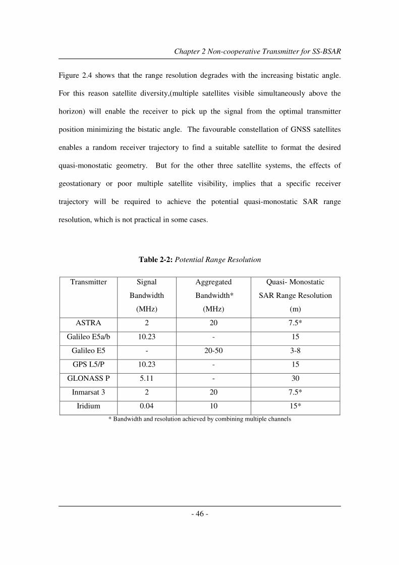
Chapter 2 Non-cooperative Transmitter for SS-BSAR
- 46 -
Figure 2.4 shows that the range resolution degrades with the increasing bistatic angle.
For this reason satellite diversity,(multiple satellites visible simultaneously above the
horizon) will enable the receiver to pick up the signal from the optimal transmitter
position minimizing the bistatic angle. The favourable constellation of GNSS satellites
enables a random receiver trajectory to find a suitable satellite to format the desired
quasi-monostatic geometry. But for the other three satellite systems, the effects of
geostationary or poor multiple satellite visibility, implies that a specific receiver
trajectory will be required to achieve the potential quasi-monostatic SAR range
resolution, which is not practical in some cases.
Table 2-2: Potential Range Resolution
Transmitter Signal
Bandwidth
(MHz)
Aggregated
Bandwidth*
(MHz)
Quasi- Monostatic
SAR Range Resolution
(m)
ASTRA 2 20 7.5*
Galileo E5a/b 10.23 - 15
Galileo E5 - 20-50 3-8
GPS L5/P 10.23 - 15
GLONASS P 5.11 - 30
Inmarsat 3 2 20 7.5*
Iridium 0.04 10 15*
* Bandwidth and resolution achieved by combining multiple channels

Chapter 2 Non-cooperative Transmitter for SS-BSAR
- 47 -
0 20 40 60 80 100 1200
5
10
15
20
25
30
Bistatic Angle (degree)
Range R
esolu
tion (
m)
Iridium
ASTRA or Inmarsat 3
Galileo
Figure 2.4: Range Resolution vs Bistatic Angle
Table 2-3: Calculation Parameters
Transmitter to target centre range 20000 km
Transmitter incident angle 45 degree
Transmitter speed 3000 m/s
Receiver altitude 500 m
Receiver speed 10 m/s
Integration time 100 s
Signal bandwidth 10.23 MHz
Monostatic range resolution 15 m
Carrier frequency 1191.795 MHz (Galileo E5)
Earlier works by Willis [5], Jones [6] derived the traditional bistatic radar resolution
using a geometrical method, similar to equation 2.9 derived above. There is another
method, vector gradient, used by Cardillo [7] to define bistatic SAR range and Doppler

Chapter 2 Non-cooperative Transmitter for SS-BSAR
- 48 -
resolution. This approach provides a more consistent way to derive the resolution without
the need for the approximations used in earlier works. This method will be applied to a
typical SS-BSAR geometry example, given in Figure 2.5. Table 2.3 gives the parameters
necessary for the resolution calculation. Iso-contours and bistatic resolution are derived
and plotted in Figure 2.6.
Figure 2.5: 2D Bistatic Geometry
Figure 2.6 shows the contours with constant range (thick line in blue) and Doppler (thin
line) on the ground plane, parallel to the earth’s surface. Figures 2.6(a) and 2.6(b) are for
the conventional monostatic SAR and quasi-monostatic SAR with stationary receiver, to
provide the comparison with the bistatic SAR case. The coordinate origin in the centre
denotes the receiver position and the arrow indicates the receiver velocity. Figures 2.6(c)
and 2.6(d) are for bistatic SAR with parallel transmitter and receiver paths and general
(non-parallel) paths, as shown in Figure 2.5. It is clearly shown in Figure 2.6(d) that
range contours become asymmetric for the non-parallel case due to large bistatic angle

Chapter 2 Non-cooperative Transmitter for SS-BSAR
- 49 -
but Doppler contours remain similar in both parallel and non-parallel cases. This is
because of the large difference in transmitter-to-target and receiver-to-target slant range,
giving a ratio of 20000 km to 1500 m. Hence the bistatic range is dominated by the
transmitter-to-target slant range; and the Doppler shift (equivalent angular speed) would
be dominated by the receiver motion.
-60
-60
-60
-40
-40 -40
-40
-20
-20 -20
0 0 0 0
20
20 20
40
40 40
40
60
60
60
X(m)
Y(m
)
-1000 -500 0 500 1000-1000
-800
-600
-400
-200
0
200
400
600
800
1000
(a) monostatic SAR
-0.5 -0.5 -0.5
-0.4 -0.4 -0.4
-0.3 -0.3 -0.3
-0.2 -0.2 -0.2
-0.1 -0.1 -0.1
0 0 0 0
0.1 0.1 0.1
0.2 0.2 0.2
0.3 0.3 0.3
0.4 0.4 0.4
0.5 0.5 0.5
X(m)
Y(m
)
-1000 -500 0 500 1000-1000
-800
-600
-400
-200
0
200
400
600
800
1000
Receiver
(b) quasi-monostatic SAR – stationary
receiver
-30-20
-20
-10
-10
-10
0 0 0 0
10
10
10
20
20
30
X(m)
Y(m
)
-1000 -500 0 500 1000-1000
-800
-600
-400
-200
0
200
400
600
800
1000
(c) SS-BSAR – parallel paths
50
60
60
60
7070
70
8080
80
90
90
90
100
X(m)
Y(m
)
-1000 -500 0 500 1000-1000
-800
-600
-400
-200
0
200
400
600
800
1000
(d) SS-BSAR – non parallel paths
Figure 2.6: Bistatic Image Grid: Iso-range Contours and Iso-Doppler Contours
Figure 2.7 shows bistatic resolution and ground resolution for the SS-BSAR parallel
paths case. The ground projection for both range and azimuth resolutions degrade
slightly because of the relatively small bistatic angle in this case. Similar to the Doppler

Chapter 2 Non-cooperative Transmitter for SS-BSAR
- 50 -
contours plotted above, azimuth resolution is mainly decided by receiver speed and the
direction of motion. Considering the short integration time, SS-BSAR with parallel paths
may be considered similar to the quasi-monostatic SAR case and Equation 2.5 could be
used to approximately define azimuth resolution.
14.8
14.8
15
15
15
15.215.2
15.2
15.215.2
15.415.4
15.4
15.415.4
15.4
15.6
15.6
15.6
15.6
15.8
15.8
16
16
16.2
16.2
X(m)
Y(m
)
-1000 -500 0 500 1000-1000
-800
-600
-400
-200
0
200
400
600
800
1000
(a) bistatic range resolution
17.5
17
.5
17.5
18
18
18
18
18.5
18
.5
18.5
19
19
19
19.5
19.5
19.5
20
20
20
20.5
20.5
20.5
21
21
X(m)
Y(m
)
-1000 -500 0 500 1000-1000
-800
-600
-400
-200
0
200
400
600
800
1000
(b) bistatic ground range resolution
0.2
0.25
0.25
0.3
0.3
0.3
0.35
0.35
0.35
0.35
0.4
0.4
0.4
0.4
0.4
0.45
0.45
0.4
5
0.45
0.45
0.5
0.5
0.5
0.5
0.5
0.5
0.55
0.5
5
0.5
5
0.55
0.6
0.6
0.6
0.65
0.65
X(m)
Y(m
)
-1000 -500 0 500 1000-1000
-800
-600
-400
-200
0
200
400
600
800
1000
(c) bistatic azimuth resolution
0.2
0.25
0.25
0.3
0.3
0.3
0.35
0.35
0.35
0.35
0.40.4
0.4
0.4
0.45
0.45
0.4
5
0.45
0.45
0.50.5
0.5
0.5
0.50.5
0.55
0.55
0.55
0.5
5
0.5
5
0.55
0.6
0.6
0.6
0.65
0.65
X(m)
Y(m
)
-1000 -500 0 500 1000-1000
-800
-600
-400
-200
0
200
400
600
800
1000
(d) bistatic ground azimuth resolution
Figure 2.7: Bistatic Resolution – Parallel Paths Case
Figure 2.8 below shows the bistatic resolution and the ground resolution for the SS-
BSAR non-parallel paths case. The ground projection for range resolutions degrades

Chapter 2 Non-cooperative Transmitter for SS-BSAR
- 51 -
substantially due to the large bistatic angle in this case. But azimuth resolution and its
ground projection are still mainly dominated by the receiver speed and direction of
motion.
20
20
22
22
2224
24
24
24
26
26
26
26
28
28
28
30
30
X(m)
Y(m
)
-1000 -500 0 500 1000-1000
-800
-600
-400
-200
0
200
400
600
800
1000
(a) bistatic range resolution
50 50 50
100 100
100
100
150
15020
0
250
300
350
X(m)
Y(m
)
-1000 -500 0 500 1000-1000
-800
-600
-400
-200
0
200
400
600
800
1000
(b) bistatic ground range resolution
0.2
0.25
0.25
0.3
0.3
0.3
0.35
0.3
5
0.35
0.4
0.4
0.4
0.4
0.45
0.45
0.4
5
0.45
0.45
0.50.5
0.5
0.5
0.50.5
0.55
0.5
5
0.55
0.55
0.6
0.6
0.6
0.65
0.6
5
0.65
0.7
0.7
X(m)
Y(m
)
-1000 -500 0 500 1000-1000
-800
-600
-400
-200
0
200
400
600
800
1000
(c) bistatic azimuth resolution
0.2
0.25
0.25
0.3
0.3
0.3
0.35
0.3
5
0.35
0.4
0.4
0.4
0.4
0.45
0.450
.45
0.45
0.45
0.5 0.5
0.5
0.5
0.50.50.55
0.55 0.55
0.5
5
0.5
5
0.55
0.6 0.6
0.6
0.6
0.6
0.65
0.6
5
0.65
0.7
0.7
X(m)
Y(m
)
-1000 -500 0 500 1000-1000
-800
-600
-400
-200
0
200
400
600
800
1000
(d) bistatic ground azimuth resolution
Figure 2.8: Bistatic Resolution – Non Parallel Paths Case
2.4 Power Budget
This section presents the power budget analysis for the proposed SS-SAR system when
utilising a transmitter of opportunity. To identify the optimal non-cooperative

Chapter 2 Non-cooperative Transmitter for SS-BSAR
- 52 -
transmitter, the parameters, such as transmitter power output, equivalent isotropical
radiated power (EIRP), will be discussed and compared using the information from the
different satellite systems. The proposed SS-BSAR system consists of two receiving
channels: the channel to receive direct signal and the channel to receive the reflected
signal. Hence the power budget of both channels will be discussed separately.
2.4.1 EIRP and Minimum Received Power
The first two parameters required in a power budget calculation are the power transmitted
by the transmitter and the power available on, or near, the receiver or target area. In radio
communication systems, EIRP is the amount of power that would have to be emitted by
an isotropic antenna (that evenly distributes power in all directions and is a theoretical
construct) to produce the peak power density observed in the direction of maximum
antenna gain. EIRP can take into account the losses in the transmission line and
connectors and includes the gain of the antenna. The EIRP allows comparisons to be
made between different transmitters regardless of type, size or form. From the EIRP, and
with knowledge of an antenna's gain, it is possible to calculate the actual power and field
strength values.
T f aEIRP P L G= − + (2.10)
where EIRP and TP (power output of transmitter) are in dBm, cable losses (
fL ) is in dB,
and antenna gain (aG ) is expressed in dBi, relative to a (theoretical) isotropic reference
antenna.

Chapter 2 Non-cooperative Transmitter for SS-BSAR
- 53 -
In general, the EIRP coverage of a GNSS signal produces a uniform power flux density
on the earth’s surface; however, this is not the case for most of the broadcasting and
communications satellites. One can expect about 5-6 dB signal power difference between
the communications satellite’s antenna beam centre and the edge of the beam. Some
communications satellites, like Inmarsat 3, are equipped with both a global beam and a
spot beam. The spot beam normally provides about 8-9 dB higher signal power than
using the global beam.
Table 2-4: Transmitter’s Parameters
Transmitter Power
output (W)
EIRP
(dBW)
Orbit Altitude
(km)
Power Density
(dBW/m2)
Galileo 50 32 23222 -126
GPS 50 30 20180 -127
GLONASS 50 28 19130 -128
ASTRA - 51 35786 -111
Inmarsat 3 - 39 35786 -123
Iridium - 21 785 -108
Table 2.4 shows the main parameters relating to signals radiated by GNSS and other
satellite systems. The values are based on free space propagation and the global beam is
considered. All three GNSS systems generate more, or less, the same EIRP with the
latest Galileo having 4 dB higher EIRP than GLONASS. Furthermore, ASTRA and
Iridium generate a much stronger power flux density than the other candidates. This is
due to its higher EIRP and lower orbit altitude.

Chapter 2 Non-cooperative Transmitter for SS-BSAR
- 54 -
From this information, the power density ( ρ ) of the satellite signals on the earth’s
surface can be derived. The calculation assumes that a receiver is located in the main
lobe of the satellite antenna beam. The flux through a 1 m2 area on the earth’s surface,
over the entire signal bandwidth, will be
24 T
EIRP
Rρ
π= (2.11)
where TR is the distance from the satellite to the receiver or target, which varies with
satellite elevation. However, the GNSS transmitting antenna produces a beam that is
slightly weaker at the centre (causing EIRP to vary with elevation), which is designed to
compensate for variations in the power received by a standard antenna. For example, the
Galileo EIRP mask boundaries within the visible Earth coverage [8] shows 2 dBW
isoflux height differences from end-of-coverage (EOC) EIRP to centre EIRP.
For GNSS systems, power flux density also can be derived from the satellite system
specification, which quotes a minimum power received using an antenna with a
nominated effective area. The power density of the satellite signals on the surface of the
earth is r
e
P
Aρ = , where rP is the guaranteed minimum signal power levels for directly
received signals and eA is the effective area of receiving antenna. The guaranteed
minimum signal power levels for three GNSS systems are specified in Table 2-5 below.
It is assumed that the signal power level is measured at the output of a linearly polarized
receiving antenna with a gain of 0 dBi, the angle of elevation is at least 10°, and

Chapter 2 Non-cooperative Transmitter for SS-BSAR
- 55 -
atmospheric attenuation is 2 dB. From Table 2-5, we can see that the three GNSS
systems have exactly same power output but slight different EIRP and power density; this
is mainly due to the difference in the transmitting antenna specification and the orbit
altitude. In terms of minimum received power and signal bandwidth, Galileo and the new
GPS L5 will provide more flexibility for target detection compared to other GNSS
signals.
It is also worth noting that the received signal power is changing with the different
satellite elevations. The received GLONASS L1/L2 signal power level for a user located
on the ground, as a function of satellite elevation angle is shown in Figure 2.9 [9]. The
highest received power level can be expected from the satellites at about 50° elevation
angle. This is due to many reasons, such as deviation (within admissible range) from
nominal orbit altitude; different values of gain of satellite transmitting antenna in
different azimuths and frequency band; accuracy of angular orientation of the satellite;
variations in output signal power due to technological reasons, temperature, voltage and
gain variations, and variations in atmospheric attenuation [10].

Chapter 2 Non-cooperative Transmitter for SS-BSAR
- 56 -
-168
-166
-164
-162
-160
-158
-156
-154
10 15 30 45 60 75 90
Angle of elevation (deg)
Po
wer
lev
el (
dB
W)
L1
L2
Figure 2.9: Relationship between Minimum Received Power Level and Elevation Angle
for GLONASS

Chapter 2 Non-cooperative Transmitter for SS-BSAR
57
GNSS Galileo GPS GLONASS
Channel E5a/b E6 E1 L1 L2 L5 L1 L2
Central
Frequency
(MHz)
1191.795 1278.75 1575.42 1575.42 1227.60 1176.45 1602.5625-
1615.5
1246-1257
Chip Rate
(M/s)
10.23 5.11 2.04 C/A: 1.023
P-code: 10.23
P-code: 10.23 10.23 C/A: 0.511
P-code: 5.11
P-code: 5.11
Antenna
gain (dBi)
15 15 15 13.5 13.5 - 11 11
Beam
width 38°-40° 38°-40° 38°-40° 38° 38° 38° 36° 36°
Power
output (W)
50 50 50 50 50 - 50 50
EIRP
(dBW)
29.7 29.7 29.5 26.5 26.5 - 25-27 25-27
Min power
received
(dBW)
-155 -155 -157 -158 -158 -154.9 -161
-167
Table 2-5: Parameters of GNSS Satellite Transmitters

Chapter 2 Non-cooperative Transmitter for SS-BSAR
58
2.4.2 The Heterodyne Channel
Usually in a radar signal processor, the range compression consists of a correlation (or
matched filtering) of the radar channel signal with the heterodyne channel signal delayed
for each range resolution cell. The performance of the matched filter depends on the
quality of the heterodyne channel signal. Ideally, one would like the signal to be as clean
as possible, i.e. free from corruption. Unfortunately, the heterodyne signal will be
spoiled by many factors, which include receiver noise, propagation distortions, multipath,
clutter, and interference. At best, one might get a heterodyne signal from a line-of-sight
direct path relatively free from interference, multipath and clutter. In this case, only the
noise in the heterodyne channel corrupts the signal. Retzer and Thomas [11, 12] have
comprehensively investigated the effect of an imperfect heterodyne signal on the
synchronisation for bistatic radar. They showed that matched filtering losses are
negligible for the heterodyne channel signal having reasonably high SNR.
The power budget for the heterodyne channel is actually a communication link budget.
In the operational SS-BSAR system, a directional or omni-directional antenna could be
used for receiving the satellite signal directly over a synchronisation link (SL). The
received signal power is calculated by taking the product of the power density ρ of the
transmitting signal on the earth’s surface and the effective area eA of the receiving
antenna. The noise power referred to the system input (the antenna terminals) within the
system is defined byn s nP kT B= , where
sT is the system noise temperature and nB is the
noise bandwidth of the system. For an N-transducer cascade, the system noise
temperature is given [4] by

Chapter 2 Non-cooperative Transmitter for SS-BSAR
59
( )
1
Ne i
s a
i i
TT T
G=
= +∑ (2.12)
where aT is the antenna noise temperature, ( ) ( )( 1)e i o n iT T F= − is the effective input noise
temperature of the ith cascaded component and iG is the available gain of the system
between its input and the input of the ith cascaded component (see Chapter 5 for the
receiver architecture). The SNR before signal processing (at the input of the
correlator/matched filter) is calculated approximately by the equation
e
s n
S A
N kT B
ρ= (2.13)
If the power density of the signal, in this expression, is the minimum value expected, the
resulting SNR should be the minimum observable SNR at the input of the correlator. If
such calculations yield a low SNR less than 10 dB, it implies that the received heterodyne
signal is almost buried under the system noise at this point. This heterodyne channel
signal can’t be used directly for the correlation with the radar channel signal.
For GNSS, a noiseless replica signal can be locally generated as the signal structure and
the spreading codes are fully known. However, this locally generated signal still needs to
be synchronized (in delay, Doppler shift and phase) with the satellite signal received at
the heterodyne channel to keep all the information necessary for further signal processing
(see Chapter 4 for more details regarding the synchronisation).
For a spread-spectrum coded signal, such as the one used in GNSS, the duration of the
spreading code is much longer than the duration of the pulses used in other satellite
systems. Hence there is a SNR improvement factor due to coherent integration
Chapter 2 Non-cooperative Transmitter for SS-BSAR
60
processing of this long spreading code. This improvement is achieved between the
antenna output and the discriminator input of the synchronisation algorithm. It can then
be expressed as
OUTc
in
SNRT B
SNR= (2.14)
where the bandwidth B is the chip rate of spreading code and cT is the coherent
integration time. For example, for the GLONASS C/A-code, B is 511 kHz andcT is
1 ms, which is the length of one C/A code, so that the integration processing introduces
27 dB SNR improvement. This SNR gain will increase to 40 dB when the Galileo E5a/b
or GPS L signal considered. For other satellite systems, the product of the signal
bandwidth and the coherent integration time (normally equals to the duration of pulse) is
one and no SNR gain is obtained due to the integration. This is the inherent advantage of
a GNSS signal for synchronisation. This follows from the fact that navigation signals
were designed to be optimal for remote synchronisation.
In general, a typical synchronisation algorithm (tracking loops) requires a minimum of
10 dB SNR at the input of its discriminator. For example, with 40 dB SNR gain obtained
by integration of the Galileo E5 signal (1 ms integration time), a minimum of -30 dB
SNR will be required at the output the heterodyne channel antenna. For other satellites
(ASTRA, Inmarsat 3, Iridium), the replica signal cannot be generated locally. This is due
to the random nature of the information modulated on the transmitting signal. In this
case, the minimum required SNR at the output of the heterodyne channel antenna is to be
at least 10 dB to achieve low matched filtering loss. Figure 2.10 below shows a graph

Chapter 2 Non-cooperative Transmitter for SS-BSAR
61
“loss in match filtering (y-axis)” versus “SNR in the heterodyne channel (x-axis)” for
various expected SNR in the radar channel. This result is helpful in demonstrating the
required 10 dB SNR in the heterodyne channel for a noise reflected GNSS signal.
-30 -20 -10 0 10 20 30-35
-30
-25
-20
-15
-10
-5
0
SNR in the heterodyne channel
Loss in t
he M
atc
hed F
iltering (
dB
)
SNR in the Radar Channel :-40 dB
-70 dB
-100 dB
Figure 2.10: the Match Filtering Losses vs. the Heterodyne SNR
So the effective size eA of this heterodyne channel antenna is proportional to the
minimum SNR required for synchronisation. As mentioned above, the period of the code
sequence used in communications satellites is much less than that of pseudo-random
sequence transmitted by the navigation satellites. If utilizing the same signal bandwidth,
synchronisation with a communications satellite will require a larger size antenna than
using a navigation satellite.

Chapter 2 Non-cooperative Transmitter for SS-BSAR
62
Table 2-6: Antenna Size vs SNR in the Heterodyne Channel
Transmitter/Signal eA (m
2) Required SNR (dB)
Galileo E5 0.001 -30
GPS L5 0.001 -30
GLONASS C/A 0.02 -17
ASTRA 0.15 10
Inmarsat 3 0.3 10
Iridium 0.04 10
Using transmitter parameters from Tables 2-4, 2-5, and Equation 2.13, Table 2-6 shows
the minimum size of the heterodyne channel antenna as a function of required SNR at the
heterodyne channel. The higher SNR in the heterodyne channel required for
synchronisation purposes is achieved at the expense of increased antenna size. It should
be noted that the calculations required to generate above table does not take in to account
a number of practical problem such as propagation and receiver losses. In real situations
we can expect a further increase in the antenna size. So we will have to use high gain
directional antenna (narrow beam) for heterodyne signal reception for the other three
satellite systems, this again will introduce an extra requirement on steering the antenna to
track the satellite position to maintain it within the beam during the formation of the
synthetic aperture.
2.4.3 The Radar Channel
The SNR of the radar channel is calculated for the period of aperture synthesis,
considering targets radar cross section (RCS) independent of frequency and angle. A
Chapter 2 Non-cooperative Transmitter for SS-BSAR
63
suitable formula for monostatic SAR was derived in [4]. Indicating that the expression for
SNR after range and azimuth compression, for an active bistatic SAR, the radar equation
can be written as
2 2
1
4 4
t t er B ic
T R o s n
PG ASPRF T
N R R KT B
σ τη
π π τ= ⋅ ⋅ ⋅ ⋅ ⋅ ⋅ (2.15)
in which most of symbols have their common meanings, erA is the effective area of THE
radar channel antenna, Bσ is THE target bistatic radar cross section and η is the loss
factor. In our case 24
t t
T
PG
Rπρ= is the power flux density on the earth’s surface. The ratio
of the uncompressed signal duration ( iτ ) and the compressed signal duration ( 0τ ) is the
SNR improvement due to range compression of the image formation algorithm.
cPRF T N⋅ = is the number of azimuth samples integrated during the integration time of
aperture synthesis (which is the gain in SNR due to the azimuth compression). If we
assume the system loss factor as η and the receiver system noise bandwidth and the
transmitting signal bandwidth are matched, so that 0 1nB τ× = and taking into
account 1i PRFτ × = , an expression for the bistatic SAR SNR can be simplified as
2
1
4
er Bc
R s
AST
N R KT
σρ η
π= ⋅ ⋅ ⋅ ⋅ (2.16)
If a geostationary satellite is used or a quasi-monostatic geometry is considered for a
moving satellite case, as discussed in section 2.3, for a fixed azimuth
resolution R Raz
c R c
R RD
L V T
λ λ∆ = = = , we can deduce that
Rc
R az
RT
V
λ=
∆ (2.17)

Chapter 2 Non-cooperative Transmitter for SS-BSAR
64
hence
1
4
er B
R s R az
AS
N R KT V
σ λρ η
π= ⋅ ⋅ ⋅ ⋅
∆ (2.18)
For any GNSS system, the power density of the transmitted signal is approximately
uniform over the illuminated region of the earth’s surface; the minimum power density
values ( ρ ) are calculated, for the three GNSS systems in the section 2.4.1.
The dimensions of the aircraft’s radar channel antenna are constrained by the size of the
aircraft and by the radar performance requirements. Coverage of the observation area
demands a reasonably large beamwidth in the range direction and the effective size of the
antenna along the radar track governs azimuth resolution. It has been assumed that a
maximum effective along-track antenna dimension of about 1 m is acceptable (the
physical dimension possibly being larger to allow beam shaping), the maximum effective
elevation (or depression) dimension being 0.5 m. Hence, for the example of bistatic SAR
using a non-cooperative transmitter, the radar channel antenna with effective area
1az D m∆ = ≈ is used in the calculation.
The value of the loss factor is estimated to be η = 0.5 (taking into account the various
mechanisms which cause loss - typically absorption, beam shape loss, polarisation loss
and a processing loss due to filter mismatch). The system noise temperature sT can be
written as( )
1
Ne i
s a
i i
TT T
G=
= +∑ , where aT is the antenna noise temperature. Assume

Chapter 2 Non-cooperative Transmitter for SS-BSAR
65
290aT K= when an antenna looks on the ground and the receiver noise figure F is 1.5 dB.
The system noise temperature is considered to be 290 410F× = Kelvin.
Table 2-7: Parameters for Power Budget Calculation
Transmitter PSD
(dBW/m2)
λ (cm) eA (m
2) az∆ (m)
Galileo -126 25.2
GPS -127 20.0
GLONASS -128 18.5
ASTRA -111 2.8
Inmarsat 3 -123 18.3
Iridium -108 18.5
0.5
1
Using the parameters in Table 2-7 and considering the typical aircraft speed of 200 m/s,
Equation 2.18 can be rearranged as
1
4
er B
az s R R R R
ASk
N KT R V R V
λ σ σρ η
π
⋅= ⋅ ⋅ ⋅ ⋅ = ×
∆ (2.19)
where 1
4
er
az s
Ak
KT
λρ η
π
⋅= ⋅ ⋅ ⋅
∆. It may be convenient to consider the factor k explicitly as
the product of four elementary factors associated with the target illumination, the receiver
antenna performance, the noise power spectral density, and an overall loss factor. The
first of these is more-or-less constant for a given satellite system. The second, associated
with receiver antenna performance, may be simplified further if the antenna is rectangular
since the azimuth beamwidth is the ratio of wavelength to the effective along-track
dimension of the antenna. The power spectral density of thermal noise changes relatively

Chapter 2 Non-cooperative Transmitter for SS-BSAR
66
little, assuming a good LNA, but the density of man-made noise may change
considerably depending on the nature of the target area. The overall loss factor depends
in part on climatic conditions and to that extent may vary a good deal.
Using Equation 2.17 and 2.19, the required integration time and achievable SNR can be
calculated for different target radar cross section and receiver-to-target distance. Some
examples are presented in Table 2-8. We can see that, to obtain certain SNR, the
minimum integration time is increasing while the receiver-to-target range increases.
Table 2-8: Power Budget Calculation
Target RCS (m2) 50 50 200 200
RR (km) 3 10 3 10
Tc (s) 3.78 12.6 3.78 12.6 Galileo
SNR (dB) 15.7 10.5 21.7 16.5
Tc (s) 0.42 1.4 0.42 1.4 ASTRA
SNR (dB) 18.1 12.9 24.2 18.9
Tc (s) 2.7 9.2 2.7 9.2 Inmarsat 3
SNR (dB) 14.3 9.1 20.3 15.1
Tc (s) 2.8 9.3 2.8 9.3 Iridium
SNR (dB) 29.3 24.1 35.3 30.1
Figure 2.10 (a) and (b) show that the system SNR varies with the target distance.
Comparing four satellite systems, it can be seen that Iridium has the highest SNR due to
its low orbit height; and the targets with 50 m2
RCS can be detected at a range of 3 km
using a Galileo satellite as the non-cooperative transmitter and 200 m2
RCS targets at the
range of 11 km, considering a 13 dB SNR detection thresholds.

Chapter 2 Non-cooperative Transmitter for SS-BSAR
67
0 10 20 30 40 50 60 70 800
5
10
15
20
25
30
35
Target Detection Range (km)
Sig
nal-to
-nois
e R
atio (
dB
)
Galileo
ASTRA
Inmarsat 3
Iridium
(a) For Target with 50 m2 RCS
0 20 40 60 80 100 120 140 160 180 2000
5
10
15
20
25
30
35
40
45
Target Detection Range (km)
Sig
nal-to
-nois
e R
atio (
dB
)
Galileo
ASTRA
Inmarsat 3
Iridium
(b) For Target with 200 m2 RCS
Figure 2.11: SNR vs Target Detetion Range
Chapter 2 Non-cooperative Transmitter for SS-BSAR
68
2.5 Summary
This chapter has discussed and compared the different candidates of non-cooperative
transmitter for SS-BSAR. The analysis has been made on the basis of three important
parameters: availability of transmitters, resolution and power budget. Four different
types of satellite transmitters are considered; they are GNSS, ASTRA, Inmarsat, and
Iridium.
The equations of bistatic resolution and its ground projection have been derived. Using
the vector gradient method, iso-range and iso-Doppler contours have been plotted and the
achievable resolutions have been calculated for two different bistatic geometries, parallel
paths and non-parallel paths. The bandwidth of most GNSS navigation signals is under
10 MHz, which corresponds to 15 m, or lower, range resolution. For SS-BSAR using
GNSS, the receiver parameters will mainly determine the azimuth resolution; and the
finest ground range resolution may be obtained with quasi-monostatic topology.
It is highlighted that the GNSS satellite transmits about 10-20 dB less power compared
to other satellites. However, it has an advantage of satellite diversity. Therefore one can
choose the desired bistatic geometry for minimum range resolution loss. For example,
Direct Satellite TV (DVB-S) broadcasting transmitters introduce about 20 dB stronger
power flux density near the earth’s surface compared to GNSS transmitters. However,
geostationary satellites are fundamentally positioned above the equator and this requires a
specific receiver trajectory for mapping a particular area and, in many or even most

Chapter 2 Non-cooperative Transmitter for SS-BSAR
69
situations, a vital loss in ground range resolution may take place due to the limited
bistatic geometry.
It is also pointed out that for low match filtering loss, the heterodyne channel should have
reasonably high SNR. It is shown that for broadcasting and communications satellites
this is achieved at the expense of increased antenna size and potentially the antenna may
be impractical to be mounted on an airborne platform. For GNSS one can locally
generate the replica signal but it needs to be synchronized with the satellite transmitter.
The synchronisation requires very low SNR (-30 dB) at the output of the heterodyne
channel antenna. This makes it possible to use an omni-directional antenna for
synchronisation with an airborne receiver.
Finally, it is concluded that overall a GNSS satellite is the best non-cooperative
transmitter candidate for SS-BSAR. It provides a reasonable range resolution of ~ 3-8 m,
allows satellite diversity and a target detection range of ~ 3-12 km for targets with 50 m2
RCS.
References
1. Rodriguez-Cassola, M., et al., Bistatic TerraSAR-X/F-SAR Spaceborne–Airborne
SAR Experiment: Description, Data Processing, and Results. Geoscience and
Remote Sensing, IEEE Transactions on 2010. 48(2): p. 781 - 794
2. Walterscheid, I., et al., Bistatic SAR Experiments With PAMIR and TerraSAR-X—
Setup, Processing, and Image Results. Geoscience and Remote Sensing, IEEE
Transactions on 2010. 48(8): p. 3268 - 3279.
3. Okan, V., GPS, http://www.movingsatellites.com/.
4. Skolnik, M.I., Radar Handbook. 1990: McGraw Hill.

Chapter 2 Non-cooperative Transmitter for SS-BSAR
70
5. Willis, N.J., Bistatic Radar. 1991: Artech House.
6. Jones, H.M., Presicted properties of bistatic satellite images, in IEEE National
Radar Conference. 1993. p. 286-291.
7. Cardillo, G.P., On the use of the gradient to determine bistatic SAR resolution, in
Antennas and Propagation Society International Symposium. 1990. p. 1032-1035.
8. Galileo Open Service Signal In Space Interface Control Document. 2006,
European Space Agency / Galileo Joint Undertaking.
9. GLONASS Interface Control Document 2002.
10. GPS Interface Control Document. 2002.
11. Retzer, G. A concept for signal processing in bistatic radar. in IEEE International
Radar Conference. 1980.
12. Daniel, D. and J. Thomas, Synchronization of Non-cooperative Bistatic Radar
Receivers. 1999, Syracuse University.

Chapter 3 GNSS Signals for SS-BSAR Application
- 71 -
Chapter 3 GNSS Signals for SS-BSAR Application
3.1 Introduction
In the previous chapter, the potential non-cooperative transmitters for SS-BSAR were
identified and compared, in terms of the availability, the resolution and the system power
budget. The conclusion is that GNSS satellites have the advantage of large constellations
and multiple visibilities. Also, they can provide reasonable range resolution and fair SNR
after range and azimuth compression from SAR image formation.
However, GNSS signals are designed for the purpose of navigation and positioning,
instead of radar applications. For most conventional monostatic SAR, the signals are
transmitting in pulse mode without carrying extra modulated information. GNSS signals,
instead, are transmitting in a continuous wave (CW) with modulated navigation
information. The bandwidth of GNSS signals is often much smaller than that of
conventional SAR signals.
This chapter will provide an analysis of the available GNSS signals from the SAR
application point of view. Its generation, reception and power spectrum will be
discussed. More importantly, the correlation property of GNSS signals will be studied
and analysed to support the development of synchronisation and image formation
algorithms. For SS-BSAR, the potential range resolution not only depends on the
bandwidth of the ranging signal but also on the relative motion between the transmitter,

Chapter 3 GNSS Signals for SS-BSAR Application
- 72 -
receiver and target. A method will be proposed in this chapter to improve the range
resolution by combining the bandwidth of GNSS signals.
3.2 GNSS Signal Frequency Bands
Figure 3.1: GNSS Signals Frequency Bands
Figure 3.1 presents the frequency bands for three major GNSS systems. It includes both
the current GNSS signals and the future available signals. From Figure 3.1 we can see
that GNSS frequency bands are crowded with signals from each constellation and
sometimes the spectrum of adjacent signals overlap. Due to the modulation scheme, it
has no effect for the navigation and positioning. However, this may introduce in-band
interference for radar applications and affect the system SNR.
Galileo has a number of navigation signals modulated in three carriers: E5, E6 and E1.
They are indicated in blue in Figure 3.1. Three independently usable signals are
permanently transmitted by all Galileo satellites. The E5 link is further sub-divided into
two RF links, E5a and E5b, covering the total bandwidth (E5) of ~ 51 MHz. All Galileo

Chapter 3 GNSS Signals for SS-BSAR Application
- 73 -
satellites will use the same frequency bands and make use of the code division multiple
access (CDMA) technique. Spread spectrum signals will be transmitted, including
different ranging codes per signal, per frequency, and per satellite. Most Galileo signals
come in pairs: a data (navigation message) signal and a data-free signal. For example, the
E5b signal consists of two signals: E5b-I and E5b-Q. They are aligned in phase and
consequently have the same Doppler frequency. For further details please refer to section
3.3 and the document [1].
The GIOVE-A and GIOVE-B spacecrafts are the first two Galileo testing satellites
nominally providing signals on two out of the three carriers E5, E6 and E1 at a time, in
the combinations E1-E5 or E1-E6. These two satellites will be used as the non-
cooperative transmitter for SS-BSAR imaging experiments. The details of the
experiments are presented in Chapter 5.
GPS modernization will introduce new navigation signals: a second civil signal in L2, a
new carrier L5 and a new military signal M-code in L1 and L2 (shown in red in Figure
3.1). The main benefits of the new L5 signal include the improvement of signal structure
for enhanced performance with: high power (-154.9 dBW), wider bandwidth (24 MHz),
longer spreading codes in the navigation message and a data-free code to enhance the
signal performance. An essential element of GPS modernization involves sharing or the
dual use of the current L band spectrum by multiple signals that provide an enhanced
radio navigation service for civilian and military users.

Chapter 3 GNSS Signals for SS-BSAR Application
- 74 -
L1 and L2 signals of GLONASS are indicated in green in Figure 3.1. It provides two
navigation signals: C/A code and P-code, which have 511 kHz and 5.11 MHz spreading
code rate separately. GLONASS adopts the frequency division multiple access (FDMA)
technique. There is also a modernization scheme for the current GLOSNASS
constellation with new navigation signals. More information can be found in [2].
Existing GPS, a classic example of CDMA systems, currently employs non-return-to-
zero (NRZ) waveforms on the spread spectrum codes. It is well known that NRZ
waveforms concentrate the energy towards the centre of the band at the carrier frequency.
The band region away from the centre of the frequency band is not used efficiently. The
power spectral density (PSD) of NRZ signals follow a typical sinc function, which has
nulls at the multiples of the spreading code chip rate in a CDMA system.
The Galileo signals and the planned modernized GPS signals will inherit improved
performance compared to the existing GPS signals. One of the improvements is the
introduction of the binary offset carrier (BOC) modulation. Binary offset carrier
modulations offer two independent design parameters: subcarrier frequency and
spreading code rate. These two parameters provide the freedom to concentrate signal
power within specific parts of the allocated band to reduce interference with the reception
of other signals. Furthermore, the redundancy in the upper and lower sidebands of BOC
modulations offers practical advantages in receiver processing for signal acquisition, code
tracking, carrier tracking, and message demodulation.

Chapter 3 GNSS Signals for SS-BSAR Application
- 75 -
The binary offset carrier (BOC) modulation provides a simple and effective way of
moving signal energy away from the band centre, offering a high degree of spectral
separation from conventional NRZ or phase shift keyed (PSK) signals, whose energy is
concentrated near the band centre. The resulting “split spectrum signal” effectively
enables frequency sharing, while providing attributes that include simple implementation,
good spectral efficiency, high accuracy, and enhanced multipath resolution [3]. Therefore,
the combination of binary offset carrier and NRZ schemes in a given GNSS frequency
band improves the bandwidth utilization beyond what only one signalling scheme can do.
A BOC(m, n) signal is created by modulating a sine wave carrier with the product of a
pseudorandom noise (PRN) spreading code and a square wave subcarrier, each having
binary ±1 values. The parameter m stands for the ratio between the subcarrier frequency
and the reference frequency of = 1.023 MHz, and n stands for the ratio between the code
rate and of . Thus, BOC(15,10) means a 15.345 MHz subcarrier frequency and a 10.23
MHz code rate. The special case of BOC(n, n) is equivalent to Manchester code. The
transmitting signal is the product of the carrier, spreading code, binary offset carrier, and
the navigation message. Traditionally, at the reception end, the RF hardware removes the
carrier and the correlators remove the binary offset carrier code, leaving the navigation
message and the residual frequency (Doppler shift) to be extracted or measured by a
processor. More information is introduced in Chapter 4 regarding the GNSS signals
reception process.

Chapter 3 GNSS Signals for SS-BSAR Application
- 76 -
From Figure 3.1, it can be seen that there are three navigation signals that have the code
rate of 10.23 MHz (the highest in all GNSS signals), which is equivalent to a 15 m range
resolution in monostatic or quasi-monostatic SAR topology. They are GPS P-code on L1
and L2, the new GPS L5 signal and the signals carried by Galileo E5a/b. Because GPS
P-code is an encoded signal that is mainly for military use and due to the unavailable of
the L5 signal, Galileo E5 is the only signal available for a SS-BSAR imaging experiment.
The next section will give a description of its generation, reception and power spectrum.
3.3 GNSS Signals Generation and Reception
Galileo introduced the innovative signal structure Alternate Binary Offset Carrier (15, 10)
(or AltBOC (15, 10)) on its E5 signal, which aims to provide the advantages of multipath
effect reduction and narrow band interference rejection. However, conventional GNSS
receiver techniques are designed for a BPSK modulated signal. When the conventional
design is adopted by Galileo signal processing, it will experience signal loss because of
poor tracking loop (i.e. Delay Lock Loop (DLL)) stability due to the wider main lobe of
the Galileo signal frequency spectrum and the ambiguous secondary peaks on the Galileo
signal Autocorrelation Function (ACF).
The advantage of the AltBOC signal is that it provides spectral isolation between the two
upper and lower components of the same composite signal. This signal makes it possible
to retain the binary offset carrier implementation simplicity, while permitting the
differentiation of the spectral lobes. The idea of Alternate binary offset carrier

Chapter 3 GNSS Signals for SS-BSAR Application
- 77 -
modulation is used to perform the same process as binary offset carrier modulation but
the sub-carrier used is a “complex” sub-carrier (see Figure 3.2). In that way, the signal
spectrum is not split up, but only shifted to higher frequencies. Shifting to lower
frequencies is obviously also possible.
0 1 2 3 4 5 6 7
x 10-8
-2
-1.5
-1
-0.5
0
0.5
1
1.5
2
Ts/8
(a) Square wave sub-carrier for BOC
0 1 2 3 4 5 6 7
x 10-8
-1.5
-1
-0.5
0
0.5
1
1.5
Ts/8
(b) Complex sub-carrier for AltBOC
Figure 3.2: Sub-Carrier
However, the shifted signal doesn’t have a constant envelope and thus may be distorted
within the satellite payload due to non-linear amplification. That’s why an innovation
was proposed in [4] in order to create a constant envelope signal which is as close as
possible to the AltBOC signal. The innovation introduces new terms which can be
compared to intermodulation products. The expression of the new signal that has been
obtained is called constant envelope AltBOC. It is actually a classical 8-PSK modulation
with a non-constant allocation of the 8 phase-states.

Chapter 3 GNSS Signals for SS-BSAR Application
- 78 -
3.3.1 Signal Generation
For GNSS signals using BPSK modulation, the expressions can be given for the power
normalized complex envelope ( )Xs t (i.e. base-band version) of a modulated signal
( )XS t (band-pass). Both expressions are described in terms of in-phase and quadrature
components in the equations below
( ) 2 ( ) cos(2 ) ( )sin(2 )X X X I X X Q XS t P s t f t s t f tπ π− − = − (3.1)
( ) ( ) ( )X X I X Qs t s t js t− −= + (3.2)
where XP is the total available power,
X Is − and X Q
s − are the in-phase and quadrature
components, which are the product of the spreading code and the navigation bits and Xf
is the carrier frequency. To compare this to the generation of Galileo E5 AltBOC(15, 10)
modulation, Figure 3.3 below gives an example of the modulation scheme for GLONASS
signals. The L1 signal consists of a quadrature C/A code and P-code; and L2 signal only
has a P-code.

Chapter 3 GNSS Signals for SS-BSAR Application
- 79 -
Figure 3.3: GLONASS Signals Modulation Scheme
The bandpass version expression for the GLONASS L1 signal can be written as
[ ]1 1 1( ) 2 ( ) ( ) cos(2 ) ( ) ( )sin(2 )L L LS t P C t D t f t P t D t f tπ π= + (3.3)
where ( )C t and ( )P t are the spreading codes, and ( )D t is the navigation message. Its
5.11 MHz P-code can be used as the ranging signal for SS-BSAR applications. GPS
signals can be generated and expressed with the same modulation scheme and expression
given above.
The wideband Galileo E5 signal is then generated using the AltBOC modulation with a
side-band sub-carrier, which can be written as [1]

Chapter 3 GNSS Signals for SS-BSAR Application
- 80 -
( )[ ]
( )[ ]
( )[ ]
( )
5 5 5 5 5
5 5 5 5
5 5 5 5
5 5 5 5
1( ) ( ) ( ) ( ) ( / 4)
2 2
1( ) ( ) ( ) ( / 4)
2 2
1( ) ( ) ( ) ( / 4)
2 2
1( ) ( ) ( ) ( /
2 2
E E a I E a Q E S E S S
E b I E b Q E S E S S
E a Q E a Q E P E P S
E b I E b Q E P E P S
s t s t js t sc t jsc t T
s t js t sc t jsc t T
s t js t sc t jsc t T
s t js t sc t jsc t T
− − − −
− − − −
− − − −
− − − −
= + − −
+ + + −
+ + − −
+ + + −[ ]4)
(3.4)
The respective definitions of the binary spreading sequences 5E a Is − , 5E a Qs − , 5E b Is − and
5E b Qs − are the product of the spreading codes and navigation message (for 5E a Is − and
5E b Is − only). The E5 spreading codes include the primary and secondary codes. The
definition and generation of the spreading codes are included in Appendix A. The
respective dashed support sequences 5E a Is − , 5E a Qs − , 5E b Is − and 5E b Qs − are product signals,
as described in equation 3.5.
5 5 5 5 5 5 5 5
5 5 5 5 5 5 5 5
E a I E a Q E b I E b Q E a Q E a I E b I E b Q
E b I E a I E a Q E b Q E b Q E a I E a Q E b I
s s s s s s s s
s s s s s s s s
− − − − − − − −
− − − − − − − −
= =
= = (3.5)
The parameters 5E Ssc − and
5E Psc − represent the four-valued sub-carrier functions (see
Figure 3.2 (b)) for the single signals and the product signals respectively.
85 ( )
8
SE S i
i
Tsc t AS rect t i
∞
−
=−∞
= ⋅ −
∑ (3.6)
85 ( )
8
SE P i
i
Tsc t AP rect t i
∞
−=−∞
= ⋅ −
∑ (3.7)

Chapter 3 GNSS Signals for SS-BSAR Application
- 81 -
Figure 3.4: Galileo E5 Modulation Scheme
Figure 3.4 above gives the modulation scheme for Galileo E5. It can be seen that the full
E5 signals consist of two signals and four codes, in comparison to two codes on the
GPS/GLONASS L1 signal. All four codes can be used as the ranging signal for radar
applications and the correlation of only data-free 5E a Qs − or 5E b Qs − codes support a simpler
signal processing algorithm than data signals. However, usage of both I and Q signals
will increase the received power, hence SNR. For example, combining the I and Q
components of the E5b signal will improve the SNR by 3 dB compared to using E5b-Q;
and the usage of all four codes results in 6 dB higher SNR. This is a significant increase
as GNSS signals transmit relatively low signal power in terms of radar applications.

Chapter 3 GNSS Signals for SS-BSAR Application
- 82 -
3.3.2 E5 signals reception
The multiplexing of the transmission for the E5a and E5b signals gives three alternative
methods of processing the signal within the receiver architecture:
� E5a single sideband reception
� E5b single sideband reception
� E5 wideband reception
In order to simplify the processing route and to focus on the radar signal processing,
single sideband reception is recommended for an SS-BSAR imaging experiment. The
E5a or E5b signal can be received in a similar manner to a QPSK modulated signal
according to the following
5 5 5 5 5 5
5 5
5 5 5 5 5 5
( ) cos(2 ( )( ) )( ) 2
( )sin(2 ( )( ) )
E a I E a E a E a E a E ar r
E a E a
E a Q E a E a E a E a E a
s t f f ts t P
s t f f t
τ π τ φ
τ π τ φ
−
−
− − ∆ − + =
− − − ∆ − + (3.9)
where 5
r
E aP is the E5a total received power, 5E aτ is the delay between transmission and
reception for E5a, 5E af∆ is the carrier frequency offset and 5E aθ is the received phase.
After I-Q demodulation (output from receiver), its baseband components can be written
as
5 5 5 5 5
5 5 5 5 5
( ) cos(2 ( ) )( )
( )sin(2 ( ) )
E a I E a E a E a E a
E a Q E a E a E a E a
s t f tI t
s t f t
τ π τ θ
τ π τ θ
−
−
− ∆ − + =
+ − ∆ − + (3.10)

Chapter 3 GNSS Signals for SS-BSAR Application
- 83 -
5 5 5 5 5
5 5 5 5 5
( ) sin(2 ( ) )( )
( ) cos(2 ( ) )
E a I E a E a E a E a
E a Q E a E a E a E a
s t f tQ t
s t f t
τ π τ θ
τ π τ θ
−
−
− ∆ − + =
− − ∆ − + (3.11)
( )
( )5 5 5 5 5 5 5
5 5 5 5 5 5 5
( ) ( ) cos(2 ( ) )( )
( ) ( ) sin(2 ( ) )
E a I E a E a Q E a E a E a E a
E a I E a E a Q E a E a E a E a
s t s t f tI jQ t
s t s t f t
τ τ π τ θ
τ τ π τ θ
− −
− −
− − − ∆ − + + = + − + − ∆ − +
(3.12)
This baseband complex signal is the actual input signal to the synchronisation algorithm
described in Chapter 4. The parameters 5E aτ ,
5E af∆ , and 5E aθ will then be tracked and
used for local reference generation.
Nevertheless, the wideband E5 signal reception is required for the range resolution
improvement proposed in section 3.5; and it can be processed in a correlation receiver
which generates a local replica in accordance with an AltBOC signal format according to
equation 3.4.
3.3.3 Power Spectrum Density
Galileo E5 signals apply AltBOC(15 10) modulation with subcarrier frequency
15 1.023scf MHz= × and chip rate 10 1.023cf MHz= × . Neglecting its dashed support
sequences (intermodulation products), it can be simplified as (in comparison to equation
3.4)
5 5 5
5 5 5
( ) [ ( ) ( ) ( )][ (cos(2 )) (sin(2 ))]
[ ( ) ( ) ( )][ (cos(2 )) (sin(2 ))]
AltBOC E aI E aI E aQ sc sc
E bI E bI E bQ sc sc
x t C t D t jC t sign f t jsign f t
C t D t jC t sign f t jsign f t
π π
π π
= ⋅ + + +
⋅ + −

Chapter 3 GNSS Signals for SS-BSAR Application
- 84 -
(3.13)
where ( )C t are the spreading codes and ( )D t is the navigation message. To calculate the
power spectrum density of a Galileo E5 signal, different terms of cross-correlation must
be taken into account and analysed. The code sequences are independent, so the cross-
correlation between two different codes is equal to zero. Consequently, all the cross-
correlation terms in which the cross-correlation between two different codes, or different
sub-carrier, are null. So the power spectral density of AltBOC(15 10) can then be written
as the equation below according to [5]
22
2 22
cos ( )4( ) [cos ( ) cos( ) 2cos( )cos( ) 2]
2 2 2 4cos ( )
3
c s s s s
cc
fT T T T TG f f f f f
Tf Tf
ππ π π π
π π= − − +
(3.14)
-6 -4 -2 0 2 4 6
x 107
-110
-105
-100
-95
-90
-85
-80
-75
-70
-65
-60
Frequency (Hz)
Am
plit
ude (
dB
W)
PSD of AltBOC(15 10) (theory)
Figure 3.5: Power Spectrum of AltBOC(15,10)

Chapter 3 GNSS Signals for SS-BSAR Application
- 85 -
Figure 3.5 plots the power spectral density (from equation 3.14) of constant envelope
AltBOC(15, 10) modulation, which is utilized by Galileo E5 signals. It can be compared
to the power spectral density of BPSK signal and other binary offset carrier signals
plotted in Figure 3.6.
-6 -4 -2 0 2 4 6
x 107
-110
-105
-100
-95
-90
-85
-80
-75
-70
-65
-60BPSK PSD
Frequency (Hz)
Am
plit
ude (
dB
W)
(a) Power spectral density of BPSK signal, P-
code
-1 -0.8 -0.6 -0.4 -0.2 0 0.2 0.4 0.6 0.8 1
x 107
-110
-105
-100
-95
-90
-85
-80
-75
-70
-65
-60BOC(1 1) PSD (n even)
Frequency (Hz)
Am
plit
ude (
dB
W)
(a) Power spectral density of BOC(1, 1) signal,
Galileo E1
-3 -2 -1 0 1 2 3
x 107
-110
-105
-100
-95
-90
-85
-80
-75
-70
-65
-60BOC(15 10) PSD (n odd)
Frequency (Hz)
Am
plit
ude (
dB
W)
(c) Power spectral density of BOC(15, 10) signal
-3 -2 -1 0 1 2 3
x 107
-110
-105
-100
-95
-90
-85
-80
-75
-70
-65
-60Constant Envelope AltBOC(15 10) PSD
Frequency (Hz)
Am
plit
ude (
dB
W)
(d) Power spectral density of Galileo E5 signal
(constant envelope AltBOC)
Figure 3.6: PSD for Different Modulations

Chapter 3 GNSS Signals for SS-BSAR Application
- 86 -
3.4 Correlation Properties
The Pseudorandom Noise (PRN) codes are selected as the spreading sequences for the
GNSS signals because of their characteristics. The most important characteristics of the
pseudorandom noise codes are their correlation properties. These properties are
described in [6]. Among them, two important correlation properties of the pseudorandom
noise codes can be stated as follow:
� Nearly no cross correlation All the pseudorandom noise codes are nearly
uncorrelated with each other. That is, for two codes iC and kC for satellites i and
k, the cross correlation can be written as
0
( ) ( ) ( ) 0N
ik i k
n
r m C n C n m=
= + ≈∑ for all m (3.15)
� Nearly no correlation except for zero lag All pseudorandom noise codes are
nearly uncorrelated with themselves, except for zero lag. This property makes it
easy to find out when two similar codes are perfectly aligned. The autocorrelation
property for satellite k can be written as
0
( ) ( ) ( ) 0N
kk k k
n
r m C n C n m=
= + ≈∑ for m ≠ 1 (3.16)
The auto-correlation function (ACF) has a peak of magnitude
, 2 1L
kk peakr = − (3.17)
where L is the number of states in the shift registers. In this case, L is equal to 13. The
remaining values (sidelobe) satisfy the following inequality

Chapter 3 GNSS Signals for SS-BSAR Application
- 87 -
( 2) / 22 1L
kkr +≤ + (3.18)
High auto-correlation peaks and low cross-correlation peaks can provide a wide dynamic
range for signal acquisition. In order to detect a weak signal in the presence of strong
signals, the auto-correlation peak of the weak signal must be stronger than the cross-
correlation peaks from the strong signals.
Table 3-1: Sidelobe Level of Pseudorandom Noise Codes
Signal Code Length (bits) Sidelobe Level (dB)
Galileo E5a/b 10230 -40
GLONASS C/A 511 -54
GLONASS P-code 5110000 -66
GPS P-code 15345000 -72
The peak-to-sidelobe level of a pseudorandom noise code can be calculated from the
equation below.
10
120 log ( )
N× (3.19)
For the full length PRN code and for the truncated code, it is derived from
10
120 log ( )
N× (3.20)
Galileo E5a/b and GPS/GLONASS P-codes are generated from a truncated
pseudorandom noise code. GLONASS C/A code is generated from the full length
pseudorandom noise code. The sidelobe level of each code is given in Table 3-1 above.

Chapter 3 GNSS Signals for SS-BSAR Application
- 88 -
Figure 3.7 below presents the auto-correlation function (ACF) of four GNSS signals
using different modulations.
-1.5 -1 -0.5 0 0.5 1 1.5
x 10-6
-0.2
0
0.2
0.4
0.6
0.8
1
1.2ACF BPSK
Delay (s)
Norm
aliz
ed A
CF
(a) ACF of BPSK signal
-1.5 -1 -0.5 0 0.5 1 1.5
x 10-5
-0.4
-0.2
0
0.2
0.4
0.6
0.8
1ACF BOC(m n)
Delay (s)N
orm
aliz
ed A
CF
(a) ACF of BOC(1, 1) signal
-1.5 -1 -0.5 0 0.5 1 1.5
x 10-6
-0.2
0
0.2
0.4
0.6
0.8
1
1.2ACF BOC(15 10)
Delay (s)
Norm
aliz
ed A
CF
(a) ACF of BOC(15, 10) signal
-1.5 -1 -0.5 0 0.5 1 1.5
x 10-6
-0.8
-0.6
-0.4
-0.2
0
0.2
0.4
0.6
0.8
1ACF AltBOC(15 10)
Delay (s)
Norm
aliz
ed A
CF
(a) ACF of AltBOC(15, 10) signal
Figure 3.7: Auto-correlation function of BPSK and Different BOC Modulations
It can be seen that a BOC modulated signal has multiple peaks in the auto-correlation
function, in contrast to the single correlation peak of a BPSK signal. The number of
negative and positive peaks in the auto-correlation function of a BOC signal is 2 1x − ,
where2 s
c
fx
f= . For AltBOC(15, 10),
2 15.3452 1 2 1 5
10.23x
×− = × − = ; so the auto-

Chapter 3 GNSS Signals for SS-BSAR Application
- 89 -
correlation function of a AltBOC(15,10) code has five peaks. The value of i-th peak is
equal to
( 1) ( )
0, 1, ( 1)
i
i
x iX for i x
x
− −= = ± ⋅⋅⋅± − (3.21)
where 0i = is the main peak.
Figure 3.9 shows the mainlobe of the auto-correlation function for BPSK and BOC
signals in absolute value and decibel scale. The signal bandwidth is 10.23 MHz, and the
width of mainlobe is defining the resolution ability of the spreading code for radar
applications. It can be seen that the null-to-zero width of the mainlobe is 0.1 µs for
BPSK signal and is equivalent to a 15 m range resolution in the monostatic SAR case.
But the mainlobe of the auto-correlation function for a BOC signal has five peaks, which
degrades the range resolution.
-1 -0.8 -0.6 -0.4 -0.2 0 0.2 0.4 0.6 0.8 1
x 10-6
0
0.1
0.2
0.3
0.4
0.5
0.6
0.7
0.8
0.9
(a) Correlation peak for BPSK signal
-8 -6 -4 -2 0 2 4 6 8
x 10-7
-40
-35
-30
-25
-20
-15
-10
-5
(b) correlation peak in dB scale

Chapter 3 GNSS Signals for SS-BSAR Application
- 90 -
-2 -1.5 -1 -0.5 0 0.5 1 1.5 2
x 10-7
0
0.1
0.2
0.3
0.4
0.5
0.6
0.7
0.8
0.9
ACF AltBOC(15 10)
Delay
Am
plit
ude
(a) Correlation peak of 10 MHz BOC
-4 -2 0 2 4 6
x 10-7
-25
-20
-15
-10
-5
ACF AltBOC(15 10)
Delay
Am
plit
ude (
dB
)
(b) correlation peak in dB scale
Figure 3.8: Mainlobe of Correlation Peak
3.5 Resolution Enhancement
In this section, a method is proposed to improve the range resolution of GNSS signals by
combining the frequency bands. The simulation results are shown for the practical
example of the combined Galileo E5 band.
-4 -3 -2 -1 0 1 2 3 4
x 10-7
0
0.1
0.2
0.3
0.4
0.5
0.6
0.7
0.8
0.9
1Auto-correlation function
Delay (s)
Norm
aliz
ed M
agnitude
E5
E5a/E5b
(a) correlation peak of E5a/b and full E5

Chapter 3 GNSS Signals for SS-BSAR Application
- 91 -
-4 -3 -2 -1 0 1 2 3 4
x 10-7
-70
-60
-50
-40
-30
-20
-10
0Auto-correlation function
Delay (s)
Norm
aliz
ed M
agnitude (
dB
)
E5
E5a/E5b
(b) correlation peak in dB scale
Figure 3.9: Comparison of E5a/b and Full E5
Figure 3.9 above presents the mainlobe of the auto-correlation function for E5a/b signals
and the full E5 signal. If E5a/b is used as the ranging signal for SAR applications, its
resolution ability is the same as the 10 MHz BPSK signal (Figure 3.8 (b)); and its
sidelobe level is 40 dB. If full E5 is used, the main peak of the auto-correlation function
is much smaller than 0.1 µs, but its resolution is still equal to 15 m as the multiple
correlation peaks exist.

Chapter 3 GNSS Signals for SS-BSAR Application
- 92 -
-60 -40 -20 0 20 40 60-80
-70
-60
-50
-40
-30
-20
-10
0
frequency MHz
E5 Spectrum
(a) simulated E5 spectrum
-60 -40 -20 0 20 40 60-220
-210
-200
-190
-180
-170
-160
-150
-140
-130
-120
frequency MHz
Combined E5 Spectrum
(b) combined E5 spectrum (simulation)
Figure 3.10: Shifted and Combined E5 Spectrum
Figure 3.10 (a) plots the simulated E5 power spectrum. It is identical to the power
spectral density of the E5 signal derived from equation 3.14 (Figure 3.5). The simulated
E5 signal is generated according to the description in section 3.3. A method is suggested
to shift the E5a/b bands towards the centre frequency, achieving higher bandwidth, hence
a better range resolution. Figure 3.10(b) shows the power spectral density of a modified
signal after the E5a/b bands are shifted by 10.23 MHz towards the zero frequency. It can
be seen that the combined spectrum covers about 30 MHz bandwidth; and its envelope is
smoother, hence a better correlation output.

Chapter 3 GNSS Signals for SS-BSAR Application
- 93 -
-4 -3 -2 -1 0 1 2 3 4
x 1 0-7
-7 0
-6 0
-5 0
-4 0
-3 0
-2 0
-1 0
0A u to -c o rre la t io n fu n c t io n
D e la y (s )
Norm
aliz
ed M
agnitude (
dB
)
E 5 a /b
1 2 M H z
1 1 M H z
1 0 M H z
9 M H z
8 M H z
Figure 3.11: Auto-correlation Function of the Combined E5 Spectrum by Different Shifts
Figure 3.11 presents the auto-correlation function of the combined E5 spectrum, which is
from converging the original E5 band by different frequencies. The mainlobe width
becomes narrower as the shifting frequency reduces from 12 MHz to 8 MHz; but at the
same time, the sidelobe level is decreasing to less than 10 dB, which consequently
reduces the contrast of the SAR image. Balancing both mainlobe width and sidelobe
level, 10.23 MHz is the optimal amount to combine the E5 band.

Chapter 3 GNSS Signals for SS-BSAR Application
- 94 -
-4 -3 -2 -1 0 1 2 3 4
x 10-7
-70
-60
-50
-40
-30
-20
-10
0Auto-correlation function
Delay (s)
Norm
aliz
ed M
agnitude (
dB
)
shifted 10.23 MHz
E5a/b
(a) ACF of E5a/b signal and combined E5
-4 -3 -2 -1 0 1 2 3 4
x 10-7
-70
-60
-50
-40
-30
-20
-10
0Auto-correlation function
Delay (s)
Norm
aliz
ed M
agnitude (
dB
)
E5a/b
After Weighting
10.23 MHz
(b) ACF after weighting
Figure 3.12: Resolution Ability of E5a/b and Combined E5 with Frequency Domain
Weighting
Figure 3.12 again shows the auto-correlation function of E5a/b and combined E5 (shifted
10.23 MHz). It can be clearly seen that the mainlobe width has been reduced to half of

Chapter 3 GNSS Signals for SS-BSAR Application
- 95 -
the E5a/b auto-correlation peak mainlobe, hence the range resolution has improved from
15 m to 7.5 m. Figure 3.12(b) adds the results of weighting with a Kaiser window applied
in the frequency domain. It suppresses the sidelobe and at the mean time broadens the
mainlobe slightly. Looking at the frequency bands shown in Figure 3.1, a similar range
resolution enhancement may be achieved with GPS L1 and L2 signals by combining the
P-code and new M-code too.
Although the promising range resolution improvement can be expected by combining the
full E5 bandwidth, the further study and simulation will be needed to fully support this
claim. To analyse the range resolution, the CCF should be used instead of ACF. When
combining the two signals, the constant phase jump from E5a to E5b needs to be taken
into account. The phase jump in the reflected signal is different from the phase
discontinuity in the locally generated reference signal. The two signals E5a and E5b are
separated by 40 MHz and hence can have different Doppler shift. This Doppler shift
needs to be estimated and compensated before the two signals could be combined in the
real data processing. The above issues need to be addressed and confirmed by simulation
and experimentation.
3.6 Summary
This chapter provides an analysis of the available GNSS signals for potential use in radar
applications. New Galileo and modernized GPS signals are introduced and the advantage
of binary offset carrier modulation has been identified. Generation, reception, and power
spectrum have been discussed for different GNSS signals. Moreover, the correlation

Chapter 3 GNSS Signals for SS-BSAR Application
- 96 -
properties of GNSS signals have been studied and analysed. A method has been
proposed to improve the resolution by combining the bandwidth of the Galileo E5 signal.
The preliminary results of the improved resolution are presented at the end of this
chapter.
Reference
1. Galileo Open Service Signal In Space Interface Control Document. 2006,
European Space Agency / Galileo Joint Undertaking.
2. GLONASS Interface Control Document 2002.
3. Betz, J.W., Binary offset carrier modulations for radionavigation. Journal of the
institute of navigation, 2002. 48(4): p. 227-246.
4. Godet, J., Technical annex to Galileo SRD signal plans, in STF annex SRD
2001/2003 Draft 1. 2001.
5. Rebeyrol, E., et al., BOC power spectrum densities, in ION NTM 2005. 2005: San
Diego, CA. p. 769 - 778.
6. Gold, R., Optimal binary sequences for spread spectrum multiplexing. IEEE
Transactions on Information Theory, 1967. 13(4): p. 619-621.

Chapter 4 Synchronisation using GNSS Signals
- 97 -
Chapter 4 Synchronisation using GNSS Signals
4.1 Introduction
A crucial problem associated with bistatic radar is synchronisation between the
transmitter and the receiver to allow for coherent signal processing. This includes: time
synchronisation, the receiver must precisely know when the transmitter fires; phase
synchronisation, the receiver and the transmitter must be coherent over extremely long
intervals of time; spatial synchronisation, the receiving and transmitting antennas must
simultaneously illuminate the same spot on the ground [1]. SAR imaging requires precise
knowledge of the Doppler history, which in monostatic SAR can be estimated from the
raw data. However, in an opportunistic bistatic system, the lack of phase lock between
the transmitter and the receiver hinder a direct adaptation of monostatic methods. This is
further aggravated by the lack of a common time reference between the BSAR platform
position information and the acquired data.
In monostatic radar, high-frequency oscillator phase noise contributions over a very short
two-way propagation time are negligible, while for bistatic systems, oscillator phase
noise components of two frequency sources contribute to the phase shift. The effect of
oscillator phase noise on BSAR was first discussed in [2] and further investigated in [3],
which concluded that uncompensated oscillator jitter may cause a time-variant shift,
spurious sidelobe, and a deterioration of the impulse response, as well as a low-frequency
phase modulation of the focused SAR signal. Similarly, the impact of time
synchronization errors would lead to unfocused images. In explicitly designed bistatic

Chapter 4 Synchronisation using GNSS Signals
- 98 -
radars, it is usual to derive all frequencies from a common reference, for example, by
using GPS disciplined sources [4]. Another approach is to record the relative phase
offsets between the oscillators, as it will be done in the TanDEM-X mission [5], which
requires a two-way dedicated link. Once these offsets are known, they can be corrected in
the data and image processing. However, if the receiver uses a non-cooperative source of
opportunity, none of these strategies can be applied directly.
Instead, authors in [6] proposed a BSASR system with fixed receiver and spaceborne
non-cooperative transmitter. Phase synchronization and pulse-repetition frequency (PRF)
recovery are achieved using a dedicated link that receives a clean signal directly from the
satellite. How to align the acquired data with the satellite orbit and how to estimate the
Doppler centroid (DC) are studied. Similar synchronization problems, which arise in
bistatic SAR missions have also been discussed in [7, 8] and solutions for the hybrid
bistatic experiment with TerraSAR-X and PAMIR have been presented. Precise footprint
synchronization is achieved by analyzing the amplitude progression of the satellite’s
signal in order to predict the arrival time of the main beam. The second synchronization
task adjusts the receive gates to the transmit pulses which is achieved with a digital PLL.
In this chapter, the use of a dedicated synchronization link to quantify and compensate
oscillator phase noise is investigated. The synchronization link itself may also suffer
errors contributions from receiver noise, Doppler Effect, aliasing, interpolation, and filter
mismatch. Several contributions such as the influence of the ionosphere or relativistic
effects are neglected in the discussion to maintain the general overview of our approach.

Chapter 4 Synchronisation using GNSS Signals
- 99 -
4.1.1 Synchronisation for GNSS as NCT
In systems using co-operative transmitters, the transmitter and receiver can be designed
to work together, with built-in means of synchronisation. However, in non-cooperative
bistatic radar systems, the receiver has little or no knowledge of the transmitted signal,
which increases the complexity of the synchronisation problem.
As mentioned previously, BSAR is subject to problems such as spatial synchronization,
time synchronization, and phase synchronization. For the proposed SS-BSAR system
using GNSS, time synchronization is more easily achieved with a CW navigation signal
than the system transmitting a pulsed signal. There is no need for PRF recovery and
pulse alignment. As GNSS satellites mostly adopt the global beam for transmitting,
spatial synchronization is not a critical issue regarding the antenna footprint overlap.
Hence, we only discuss phase synchronization in detail in this chapter.
The receiving part of the proposed SS-BSAR consists of two channels: the radar channel
used for receiving the reflected signal from the target and the heterodyne channel used for
synchronisation with the transmitter. As discussed in Chapter 2, the heterodyne channel
signal in this case can’t directly correlate with the radar channel signal, because of its low
SNR (below the receiver noise). It is suggested that a locally generated replica should be
used, whose parameters are fully synchronized with the heterodyne channel signal.
As indicated earlier, this synchronisation process may be possible if the GNSS signal is
received directly on the heterodyne channel. Signals in the radar and heterodyne

Chapter 4 Synchronisation using GNSS Signals
- 100 -
channels are down-converted using a common local oscillator, in order to maintain the
phase relationship between the two channels, and subsequently sampled using a common
clock. A synchronisation algorithm has been proposed to apply to the stored heterodyne
signal to extract all the information needed for local replica generation. It will be
discussed in more detail in the following sections.
4.1.2 Equation of Received Signal
In this section, the equation of the received E5 signal at the heterodyne channel will be
derived, and the discussion in section 4.2 and 4.3 will be based on it. It should be noted
that, although we are considering a particular navigation signal, Galileo E5 in this
chapter, the background theory and the methods of synchronisation are generic and could
be used with other GNSS signals. The details for generation and modulation of a Galileo
E5 signal are included in Chapter 3.
As mentioned in Chapter 3, due to the multi correlation peaks of AltBOC modulation, it
is easier and more straightforward to process the E5a signal or the E5b signal separately
than correlating the full E5 signal directly. Here, we consider the E5b signal as an
example; the processing for E5a will be identical. Pseudorandom noise codes of the
Galileo E5b signal are borne by carriers in phase-quadrature. The transmitted E5b signal
at the input of the antenna can be written as:
5 5
5
5
( ( )) ( ( ))cos(2 ( ( )) ( ))( ) 2
( ( ))sin(2 ( ( )) ( ))
E b I s E b I s c s
E b
E b Q s c s
C t t D t t f t t tS t P
C t t f t t t
τ τ π τ φ
τ π τ φ
− −
−
− − − + =
− − − + (4.1)

Chapter 4 Synchronisation using GNSS Signals
- 101 -
Considering single sideband reception of the E5b, the signal received in the heterodyne
channel, after filtering, downconversion, quadrature demodulation, can be expressed as
(for example of E5b):
[ ] [ ]5 5 5[ ( )] [ ( )]cos 2 ( ) [ ( )]sin 2 ( )I E b I s E b I s s E b Q s sS C t t D t t f t t C t t f t tτ τ π φ τ π φ− − −= − − + + − +
(4.2)
[ ] [ ]5 5 5[ ( )] [ ( )]sin 2 ( ) [ ( )]cos 2 ( )
Q E b I s E b I s s E b Q s sS C t t D t t f t t C t t f t tτ τ π φ τ π φ− − −= − − + − − +
(4.3)
where 2P is the envelope of E5b signal
5 ( )E b IC t− and
5 ( )E b Q
C t− represents the spreading code of E5b
5 ( )E b ID t− is the navigation message on E5b with a chip rate of 250 bps
cf is the E5b carrier frequency
( )tφ is unknown phase variation
IS and QS are the in-phase and quadrature signals at the demodulator output
( )s tτ and sf are, respectively, the delay and carrier frequency shift suffered by
the signal from the satellite to the receiver.
The delay and frequency shift can be expressed as:
( ) ( ) ( )s d ct t tτ τ τ= + (4.4)
( ) ( ) ( )s d lof t f t f t= + (4.5)

Chapter 4 Synchronisation using GNSS Signals
- 102 -
where ( )d tτ is the varying delay due to satellite-receiver separation and ( )c tτ is the
(varying) relative time shift, which occurs due to the difference between the timing of
the receiver sampling clocks and the timing of the transmitting clock ( ( )c tτ can be
referred to as clock slippage or clock drift). The frequencies ( )df t and ( )lof t are,
respectively, the Doppler shift due to the satellite and receiver motion and the difference
between the signal’s carrier frequency and the actual frequency output of the local
oscillator ( ( )lof t is affected by the stability of oscillator). We can see that the delay and
the frequency shift are both functions of time. For example, the delay and frequency vary
due to the changing distance between the transmitter and the receiver as well as due to the
frequency drifts of the local oscillator.
4.1.3 Dynamics of Delay and Frequency Variation
From Equations 4.4 and 4.5, it is seen that both delay and frequency shift are functions of
time. The total delay τs is the sum of delay due to the satellite-receiver separation and the
time shift introduced due to unsynchronised clocks in the transmitter and receiver. Let us
first calculate the maximum delay variation due to the transmitter and the receiver motion
over an interval of one second. Figure 4.2 shows a simplified two-dimensional geometry
used for calculation. The initial position of the Galileo satellite and airborne receiver is
assumed to be (0 km, 23222 km) and (0 km, 0 km) respectively on the x-y plane. The
satellite is assumed to be moving in a straight line (in short period of time) with a
velocity of 4000 m/s in the +X direction, whereas the aircraft is moving in the negative X

Chapter 4 Synchronisation using GNSS Signals
- 103 -
direction with a velocity of 200 m/s. This indicates a rate of change of distance of
0.38 m/s, which corresponds to a delay variation about 1.3 ns per second.
23222 km
Initial position After 1 s
Initial position After 1 s
Y
X -X
200 m/s
4000 m/s
Figure 4.1: Two Dimension Geometry
The dynamics of the time-shift variation due to unsynchronised clocks depends on the
stability of the sampling clock used in the receiver. In our system we are using a clock
with a stability of 100 ppm. It was found experimentally that this clock gives an initial
time shift τc(0) of approximately 0 ms and a time variation of about 2.4 µs/s. Therefore
the total delay τs(0) is around 77 ms for 23222 km and the total delay variation is about
2.4 µs/s.
In Chapter 2 it is shown that the maximum Doppler shift due to the motion of GNSS
satellites is about 4 kHz; the maximum Doppler shift due to the movement of a low-
flying aircraft with a velocity of 200 m/s is about 1 kHz. Then a reasonable value for the
expected maximum Doppler shift is about 5 kHz. Also the expected that maximum rate-
of-change of the Doppler frequency due only to satellite motion is 1 Hz/s; its derivation is

Chapter 4 Synchronisation using GNSS Signals
- 104 -
given below. For our receiver we are using frequency synthesizers as the local oscillator
to down-convert the received signal. It was found experimentally that these oscillators
introduce some 0.5 kHz of frequency shift, which varies at the rate of ~ ±0.2 Hz/s.
Therefore the total maximum frequency shift fs(0)= 5.5 kHz. The total frequency
variation is ± 1.2 Hz/s.
It should be noted that an accurate model for estimating the delay and frequency variation
is beyond the scope of this section. Therefore the assumed delay and frequency variation
may be different for another scenario or system. Nevertheless the assumed values of the
variations give a good starting point for implementing the synchronisation algorithm.
Figure 4.2 shows a typical GNSS circular orbit around the earth, the average earth’s
radius being Re (6368 km) and Rs the GNSS satellite orbit radius. The distance RT from
the satellite to the target area varies with respect to the satellite’s elevation angle α; the
greatest distance occurs when the satellite is at the horizon; it decreases with increasing
satellite elevation angle and reaches a minimum at the zenith. The distance from the
satellite to the airborne receiver will be little different from RT, since a typical aircraft
flight altitude is less than 20 km and the GNSS satellite orbit altitude is about 20,000 km.

Chapter 4 Synchronisation using GNSS Signals
- 105 -
rs Re
α
Rs
Target
RT
RTmax
RTmin
Earth
Circular satellite orbit
0
Vs
β
00
Vd
Figure 4.2: Doppler frequency caused by satellite motion (courtesy of [9])
An expression giving the relationship between slant range (RT) and elevation (α) can be
obtained from
)90cos(2222 α+−+= TeTes RRRRR (4.8)
−
−
= αα sincos
2/1
2
2
e
s
eTR
RRR (4.9)
The maximum slant range, occurring when α = 0, is
22
max esT RRR −= (4.10)
The Doppler shift (for short observation intervals) is given by the following equation,
which is plotted below in Figure 4.3 for a GLONASS satellite. For any lateral

Chapter 4 Synchronisation using GNSS Signals
- 106 -
displacement of the target from the ground track of the satellite, the maximum Doppler
shift is observed at zero elevation.
cos cosd S e
d
S
V V Rf
R
ψ α
λ λ= = (4.11)
where ψ is the angle between the satellite’s ground track at the sub-satellite point and the
terrestrial great circle passing through this point and the target position;
0 20 40 60 80 1000
1000
2000
3000
4000
5000
6000
elevation (degree)
dop
ple
r due
to
sate
llite
mot
ion (
Hz)
0degree across track
30degree across track
60degree across track
Figure 4.3: Short Term Variation of Doppler Shift with Elevation for GLONASS
Relevant parameters are given in the Table 4-1 for the GPS L1 channel, the GLONASS
L1 channel and the Galileo E5 channel, the likely maximum Doppler referring to the
Doppler at 10 degrees elevation with no target lateral displacement. The rate-of-change
of the Doppler frequency is also important for the tracking of the GNSS signal. If the
rate-of-change of the Doppler frequency can be calculated, the frequency update rate in
the tracking algorithm can be predicted. However, the rate-of-change is not a constant
over the satellite period.

Chapter 4 Synchronisation using GNSS Signals
- 107 -
The target is assumed to be displaced normally from the satellite’s ground track by a
great circle angle φT; the satellite is displaced (along the ground track) from the point of
closest approach to the target by a great circle angle θT. The maximum rate of change of
the frequency occurs at 0Tϕ = and / 2θ π= . The corresponding maximum rate of
change of the Doppler frequency is [10]
max max 2 2
/| |
2
d Ed
E S E S
dV f VR d dt ff
dt c cR R R R
θδ = ⋅ = ⋅
+ − (4.12)
Constellation GPS GLONASS GALILEO
Orbit Period 11 hrs 58 min 11 hrs 15 min 14 hrs 22 min
Orbit Altitude (km) 20180 19130 23222
Max Range from satellite
to target on the earth’s
surface (km)
25785 24690 29300
Satellite Speed (m/s) 3874 3953 3643
Likely max. Doppler due
to sat. motion (kHz)
4.88 5.26 3.07
Max rate of change of
Doppler (Hz/s)
0.936 1.088 0.474
Table 4-1: Doppler Shift Dynamics
These two parameters will specify the synthetic aperture length and integration time
appropriate to various altitudes for different types of aircraft. Detailed calculations for
the potential resolution of SS-BSAR are given in section 2.3 using these typical values.
From that we know that the rate-of-change of the Doppler frequency caused by the
satellite motion is rather lower than due to receiver motion. It does not affect the update
rate of the tracking of synchronisation significantly. If the receiver has an acceleration of
10 m/s2 toward a satellite, the corresponding rate-of-change of the Doppler frequency can

Chapter 4 Synchronisation using GNSS Signals
- 108 -
be found from equation 4.12. The corresponding result is 53.3 Hz/s. comparing with the
rate-of-change of the Doppler shift caused by the motions of the satellite; the acceleration
of the receiver is the dominant factor. The operation and performance of a receiver
tracking loop greatly depends on the dynamics of the receiver motion.
4.1.4 Proposed Synchronisation Algorithm
It is clearly seen from Equations (4.2) and (4.3) that the locally generated pseudorandom
noise code needs to be synchronised with the received heterodyne signal in order to
decode the navigation message and generate local replica for range compression. Figure
4.4 below shows a block diagram for the synchronisation algorithm proposed. For the
example of the E5b synchronisation, it consists of:
• Acquisition, or coarse synchronisation using both in-phase and quadrature
components of the E5b signal. It estimates the coarse frequency and delay, and
extracts the secondary code.
• Frequency ( )sf t tracking using the E5b-Q. It is the pilot signal of E5b and no
navigation message is modulated. A least mean square algorithm will be applied
to remove noise effects.
• The tracked frequency is then used to remove the Doppler shift from the received
signal. The locally generated pseudorandom noise code is then fine delay
synchronised to the input signal by curve fitting methods.

Chapter 4 Synchronisation using GNSS Signals
- 109 -
• Finally, the phase variation ( )tφ is extracted and the fully synchronised local
generated pseudorandom noise code is used to decode the navigation message on
E5b-I.
• Range compression can be applied with the radar channel signal using a fully
synchronized local reference.
Acquisition
(coarse freq, delay &
2nd code)
Delay Tracking
(curve fitting
method)
Phase Tracking
Local Ref
Generation
Doppler Tracking
(medium & fine freq
estimation)
Least Mean Square
Navigation Message
Decoding
Heterodyne
Signal
Heterodyne Signal
Satellite
Coordinates
Synchronised Local Ref for
Range Compression
Figure 4.4: Synchronisation Algorithm Block Diagram

Chapter 4 Synchronisation using GNSS Signals
- 110 -
In the following two sections we will discuss the signal acquisition block and two
tracking blocks in more detail. The performance of the tracking algorithm is analysed in
terms of receiver & satellite dynamics and noise error. The results are supported by
experimentation with Galileo satellites in section 4.4.
4.2 Signal Acquisition
In order to track the parameters and decode the information on Galileo E5b signals, an
acquisition method must be used first to detect the presence of the signal. Once the
signal is detected, the necessary parameters, such as the starting bit of the pseudorandom
noise code (code phase) and coarse Doppler frequency will be obtained and passed to the
tracking program. From the tracking program, information such as fine delay, fine
Doppler and the navigation message can then be obtained.
The received signal S is a combination of signals from all n visible satellites. When
acquiring satellite k, the incoming signal S is multiplied with the local generated
pseudorandom noise code corresponding to the satellite k. The cross correlation between
pseudorandom noise codes for different satellites implies that signals from other satellites
are nearly removed by this procedure. To avoid removing the desired signal component,
the locally generated pseudorandom noise code must by properly aligned in time, that is,
have the correct phase.

Chapter 4 Synchronisation using GNSS Signals
- 111 -
Then the acquisition method must search over a frequency range to cover all likely
frequency shifts. As mentioned earlier, the Doppler frequency shift will never exceed
5 kHz for a stationary or low speed receiver on earth; and approach as high as 10 kHz
with a very high user velocity. Using a narrow bandwidth for searching means taking
many steps to cover the desired frequency range and it is time consuming. Searching
with a wide bandwidth filter will provide relatively poor sensitivity. In other words, there
is a trade-off between speed and sensitivity. If the signal is strong, the fast, low
sensitivity acquisition method can be used. If the signal is weak, the low-sensitivity
acquisition will miss it, and therefore a high sensitivity method must be employed. If the
signal is very weak, acquisition should be based on a long data length. From [9], it is
sufficient to search the frequency in steps of 1000 Hz resulting in 41 different frequencies
in the case of a fast-moving receiver and 21 in the case of a static receiver.
After mixing with the locally generated carrier wave, all signal components are squared
and summed providing a numerical value. For each of the different frequencies all
different code phases are tried. A search for the maximum value is performed. If it
exceeds a determined threshold, the satellite is acquired with the corresponding frequency
and code phase shift. Figure 4.5 below shows a typical acquisition plot for a visible
satellite. The plot shows a significant peak, which indicates high correlation.

Chapter 4 Synchronisation using GNSS Signals
- 112 -
Figure 4.5: Acquisition Result for GIOVE-A
Figure 4.6: Block Diagram (matched filter)
The different acquisition techniques have been discussed in detail and compared, in terms
of speed and sensitivity, in [9, 11]. Parallel code phase search acquisition (circular
correlation) is suggested to apply for our case. The local pseudorandom noise code is
multiplied by a locally generated carrier signal and transformed into the frequency

Chapter 4 Synchronisation using GNSS Signals
- 113 -
domain by fast Fourier transform (FFT). It’s then multiplied with the outcome of the
heterodyne signal with the FFT operation. The result of the multiplication is transformed
into the time domain by an inverse Fourier transform. If a peak is present in the
correlation, the index of this peak marks the pseudorandom noise code phase and coarse
frequency of the incoming signal. The accuracy of the estimated frequency is similar to
other acquisition methods. The pseudorandom noise code phase, however, is more
accurate as it gives a correlation value for each sampled code phase. That is, if the
sampling frequency is 50 MHz, a 1 ms code has 50000 samples, so the accuracy of the
code phase can have 50000 different values instead of 10230 (for example of E5b-I/Q).
Now let us find the integration time required to implement the correlator, shown in
Figure 4.6. The longer the integration time used, the higher the signal-to-noise ratio that
can be achieved at the output of the correlator. However, the presence of the navigation
data on the signal received from the satellite restricts the integration interval, unless this
information is known or initially extracted from the signal. This is explained as follows:
The navigation message has a data rate of 50 bps on E5a-I (250 bps on E5b-I), whereas
the E5a/b spreading codes have a bit rate of 10.23 Mbps and code length of 1 msec. Each
navigation data bit is therefore 20 ms long, so that in 20 ms of data there can be one data
transition at most. If there is a data transition in one 10 ms interval, the other 10 ms
interval will not have one. Therefore, in order to guarantee there is no transition in the
data, one of two consecutive intervals of 10 ms should be used; in practice both can be
used since the one with no transition will provide better correlation than the other.

Chapter 4 Synchronisation using GNSS Signals
- 114 -
And due to AltBOC modulation on the E5 signal, there is one extra consideration needed
for its acquisition, which is the secondary code. It splits the E5a and E5b spectrum to the
opposite side of E5 carrier frequency. It has a similar effect as the navigation message on
the acquisition and tracking algorithm. However, as the structure and length of this code
is known, it is possible to be removed by the multiplication of its local replica as long as
the code phase is aligned. For example E5b-Q, is 100 bits long with chip rate of
1000 Hz. 100 code phase transitions have to be completely tried to search the correct
code phase for E5b-Q signal. Because there is only one 4-bit secondary code on E5b-I
(remember E5b-I has navigation messages), the quickest way to search the correct
secondary code phase is using E5b-I first then search E5b-Q; only 29 (4+100/4) different
code phase transitions search will be necessary.
4.3 Signal Tracking
The acquisition provides only rough estimates of the frequency and code phase
parameters. The main purpose of tracking is to refine these values, keep track, and
demodulate the navigation message from the specific satellite. It consists of two tracking
loops. First, the pseudorandom noise code is removed from the input signal and the
frequency of the remaining CW is fine estimated; second, the estimated fine frequency
variation is then used to remove the frequency shift from the heterodyne signal,
Thereafter, fine code delay (phase) of the heterodyne signal can be found. Finally, the
phase variation is tracked and the synchronised locally generated pseudorandom noise
code can be used to decode the navigation message.

Chapter 4 Synchronisation using GNSS Signals
- 115 -
4.3.1 Fine Code/Delay Tracking
In this section two tracking methods will be discussed, the first being the conventional
tracking loop [9, 12] and the second being the method known as block adjustment of
synchronising signal (BASS). This method is suggested to be used for tracking the
heterodyne signal in our case and is therefore discussed comprehensively.
The input signal is digitised at 50 MHz, so that every sample point is separated by 20 ns,
and the coarse code phase (delay) estimate measures the beginning of the pseudorandom
noise code with this resolution. For a more accurate estimate of the delay variation (for
accurate clock recovery) additional processing is needed, as described below.
As in the block adjustment of synchronising signal algorithms, correlation is performed
on consecutive blocks of input data. The selection of the integration time in this process
is a trade-off between the requirements of the dynamics of delay variation and the SNR
of the input signal. The criteria used for selecting the delay update, for the system under
consideration, are described after discussion of the fine delay estimation algorithm.
In this section we are using a curve fitting method to estimate the fine delay as described
by [9]. Figure 4.7 below shows the mainlobe of the correlation function within one chip
of the pseudorandom code. Three correlations values are shown in this Figure: yp is the
coarse delay estimate (also known as prompt), ye is the estimate obtained from the early
code, and yl the estimate from the late code. The time t is measured from the prompt

Chapter 4 Synchronisation using GNSS Signals
- 116 -
output to the early or to the late code output. We assume that yp is tp seconds from the
ideal peak. A quadratic equation to model the correlation peak can be written as:
cbtaty ++= 2 (4.13)
where y represents the correlation value and t represents time.
t
yl yp
ye
Correlation
output
tp te= tp-d
t' t
'
te= tp+d 0
Figure 4.7: Correlation Output of a pseudorandom noise Code
This equation can be solved to obtain a, b, and c with three pairs of t and y values as:

Chapter 4 Synchronisation using GNSS Signals
- 117 -
A
1
1
1
T
Y
hTA witY
or
1
1
1
2
2
2
2
2
2
=
=
=
=
=
c
b
a
tt
tt
tt
y
y
y
c
b
a
tt
tt
tt
y
y
y
ll
pp
ee
l
p
e
ll
pp
ee
l
p
e
(4.14)
The solution can be written as:
1A T Y−= (4.15)
where T-1
is the inverse of matrix T. Once a,b,c from Equation (4.15) are found, the
maximum value of y can be found by taking the derivative of y with respect to x and
setting the result to zero. The result is:
p2 0 or t2
p
dy bat b
dx a
−= + = = (4.16)
Thus, tp is the desired fine delay estimate.
In the presence of noise it is impractical to use the tp value from a 1 ms length of data.
Although 1 ms integration time is enough for detecting the pseudorandom noise code, the

Chapter 4 Synchronisation using GNSS Signals
- 118 -
fine delay estimate tp will fluctuate from its true value due to the presence of noise. For
the system being considered, the delay estimate xp is calculated every millisecond. Every
5 ms the tp values are averaged to generate the final estimate of the delay. It was shown
in section 4.1 that the delay variation is around 2.4 µs/s for the system considered here. It
takes approximately 4.2 ms to shift the pseudorandom noise code by half the sample
interval of 20 ns, which can justify this update rate. Note that the main contributor to
delay variation is clock slippage and that the clock used in the experimental receiver does
not exhibit very high frequency stability (only 100 ppm). The dynamics of the delay
variation can be dramatically reduced if a very stable clock is used, allowing more values
of tp to be averaged to give a better delay estimate.
4.3.2 Fine Doppler Tracking
The purpose of the fine Doppler tracking algorithm is to estimate the carrier frequency of
the input signal and; phase lock loops (PLL) or frequency lock loops (FLL) are often
used. It requires two loops coupled together (one to strip off the pseudorandom noise
code and the other to estimate the frequency). However, the implementation of the code
and carrier tracking in the block adjustment of synchronising signal algorithm is different
from the conventional tracking loop method. No initial phase adjustment is required,
such as in the conventional phase-locked loop. The output from the acquisition algorithm
can be used in reducing the computation time and ambiguities in estimating the frequency
variation.

Chapter 4 Synchronisation using GNSS Signals
- 119 -
The BASS method operates on blocks of input data, the lengths of which depend on the
SNR and the dynamics of the parameters to be tracked; block lengths of 6 ms are
considered in this section.
The first step is to remove the pseudorandom noise code from the block of input data to
produce a CW signal and this is followed by a Discrete Fourier Transform (DFT). The
DFT frequency component with the greatest magnitude represents a coarse frequency
estimate of the input signal frequency. A fine frequency estimate is obtained by
comparing the phases of the frequency components identifying coarse frequency
estimates in two consecutive data blocks. In the following we discuss the pseudorandom
noise code removal and fine frequency estimation in detail.
Input signal
PRN code
Output signal
Figure 4.8: pseudorandom noise Code Wipe-off

Chapter 4 Synchronisation using GNSS Signals
- 120 -
Step 1: Stripping RPN code from the input signal
As mentioned earlier, the product of the pseudorandom noise code (with correct code
phase) and the input signal produces a CW signal, as shown in Figure 4.8 above. The top
plot is the input signal, which is a sinusoidal signal phase coded by a pseudorandom noise
code. The bottom plot is a CW signal representing the result of multiplying the input
signal and the pseudorandom noise code; the corresponding signal spectrum is no longer
spread.
The frequency of the CW signal can be found from the Fast Fourier Transform (FFT)
operation which, for an input data length of 1 ms, will have a frequency resolution of
1 kHz. A threshold can be set to identify strong components, the strongest giving a
coarse estimate of the input frequency. As mentioned earlier, the signal is digitised at 50
MHz, so that 1 ms of data contains 50,000 data points and the corresponding FFT
generates 50,000 frequency components. However, only the first 25,000 components
contain useful information, the last 25,000 being complex conjugates of the first 25,000
points. The frequency resolution is 1 kHz and the total frequency covered by the FFT is
25 MHz, which is half of the sampling frequency. As discussed earlier, the expected
maximum Doppler shift is about 5 kHz and the frequency shift of the local oscillator used
is about 500 Hz so the total frequency shift is around 5.5 kHz. The frequency range of
the FFT which is of interest is therefore only 6 kHz and only 6 frequency components
need be calculated, using the discrete Fourier Transform (DFT). The choice of method
depends on the speed of two operations.

Chapter 4 Synchronisation using GNSS Signals
- 121 -
The start of the pseudorandom noise code in the input data is unknown and, in order to
find it, the input data must be multiplied point-by-point by a locally-generated digitized
pseudorandom noise code, an FFT or DFT being performed on the product to find the
frequency.
In order to search for a suitable 1 ms block of data, the input data stream must be
progressively delayed with respect to the locally generated code, one sample interval at a
time (50,000 shifts in all). Use of the FFT requires 50,000 operations each consisting of
a 50,000-point multiplication and 50,000-point FFT. The output is 50,000 frames of data,
each containing 25,000 frequency components (because only 25,000 frequency
components provide information, the others being redundant) giving a total of 1.25 × 10⁹
components in the frequency domain; the component with the highest amplitude among
these can be considered as the desired result if it also crosses the ‘adequate strength’
threshold. Searching for the highest amplitude component can be time consuming but,
since only 6 frequencies of the FFT output are of interest, the space to be searched can be
reduced to 300,000 components. This approach allows the start of the pseudorandom
noise code to be found with a time resolution of 20 ns (1/50 MHz), the associated
frequency resolution being 1 kHz. It is clear that this process can be very time
consuming; methods used to reduce further the number of frequency outputs are
discussed below.
If one uses the initial estimate, from the acquisition program, of the relative time at which
the pseudorandom noise code period begins, the number of frequency outputs can be
Chapter 4 Synchronisation using GNSS Signals
- 122 -
reduced dramatically. As discussed in section 4.1, the delay variation is around 2.40 µs/s
(or 120 samples/second). If the delay of the pseudorandom noise code is continuously
adjusted from one block of data to another, then one need not search through all 50,000
samples every 1 ms. Ideally a search through only 1-2 samples every millisecond is
needed but, in the algorithm implemented, the search is through 6 samples every
millisecond which accommodates sudden changes (if any) in delay variation. In this case
the total number of frequency outputs is 36, which clearly reduces the computational load
significantly.
Step 2: Fine Frequency Estimation
Use of the DFT (or FFT) to find fine frequency is inappropriate because a fine frequency
resolution implies a long data record (a resolution of, say, 10 Hz requiring a data record
of 100 ms) involving a large transform (a 100 ms. record requiring a 5000,000 point
transform) which could be very time consuming. Besides, the probability of having a
phase shift in 100 ms of data is relatively high.
The block adjustment of synchronising signal approach to finding fine frequency
resolution is by phase measurement. Once the pseudorandom noise code is stripped from
the input signal, the input becomes a (digitized) CW signal x(n), the DFT output X(k) of
which can be written as:
∑−
=
−=1
0
/2)()(
N
n
NnkjenxkX
π (4.17)

Chapter 4 Synchronisation using GNSS Signals
- 123 -
in which k identifies a particular frequency component and N is the total number of data
points. The strongest frequency component in 1 ms of data at time m can be identified as
Xm(kmax) The initial phase θm(kmax) of the input can be found from the DFT output as:
( )( )
= −
)(Re
)(Imtan)(
max
max1
maxkX
kXk
m
m
mθ (4.18)
where Im and Re represents the imaginary and real parts, respectively. Let us assume
that at time n, a short time after m, the DFT component Xn(kmax) of 1 ms of data is also
the strongest component, because the input frequency will not change rapidly during a
short time. The initial phase angle of the input signal at time n and frequency component
kmax is:
( )( )
max1
max
max
Im ( )( ) tan ,
Re ( ) 2 2
n
n
n
X kk
X k
π πθ θ−
= − < <
(4.19)
The two phase angles can be used to find the fine frequency as:
)(2
)(k)( maxmax
mn
kf mn
−
−=
π
θθ (4.20)
Figure 4.9 below diagrammatically represents Equation (4.20). This equation provides a
much finer frequency resolution than the result obtained from the DFT. In order to keep
the frequency unambiguous the phase difference )()( kmkn θθ − must be less than 2π. If
the phase difference is at a maximum value of 2π, the unambiguous bandwidth is 1/(n-m)
where n-m is the delay time between two consecutive data sets.
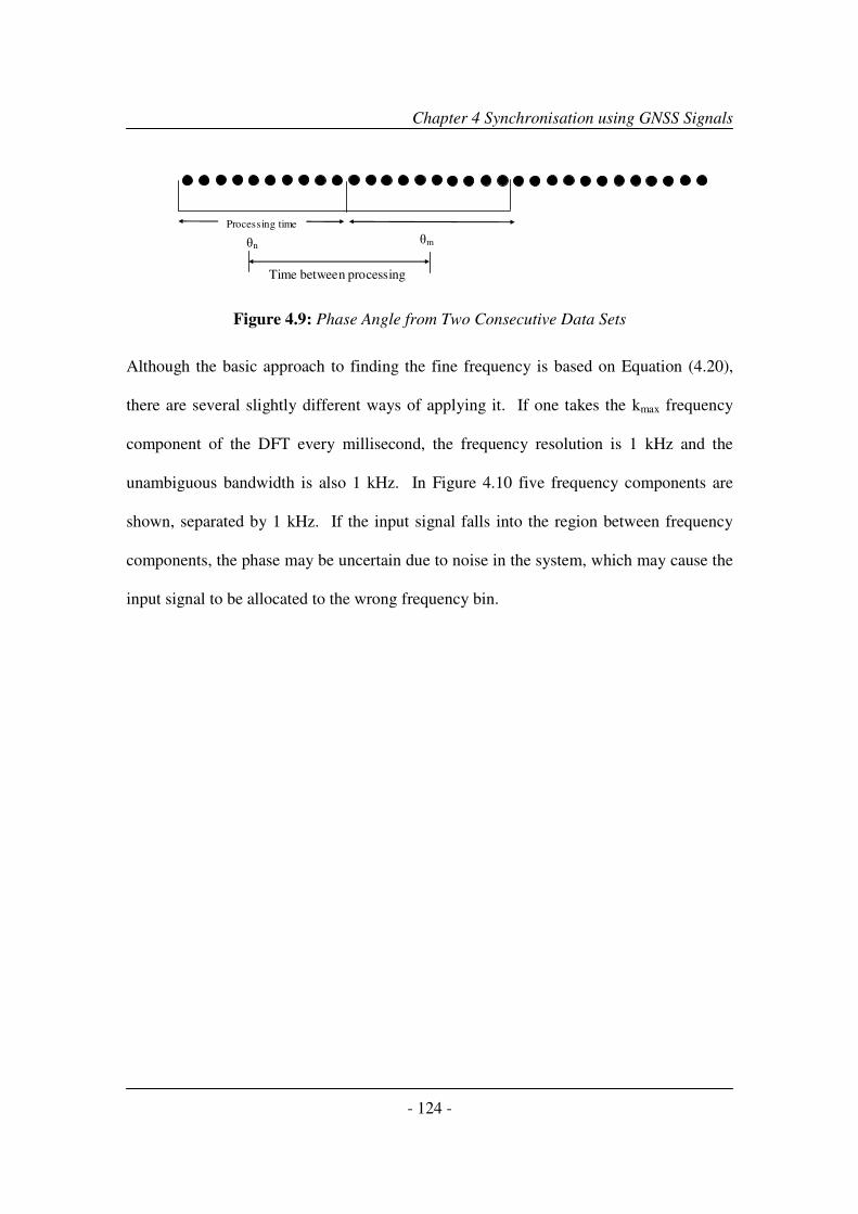
Chapter 4 Synchronisation using GNSS Signals
- 124 -
Processing time
θn θm
Time between processing
Figure 4.9: Phase Angle from Two Consecutive Data Sets
Although the basic approach to finding the fine frequency is based on Equation (4.20),
there are several slightly different ways of applying it. If one takes the kmax frequency
component of the DFT every millisecond, the frequency resolution is 1 kHz and the
unambiguous bandwidth is also 1 kHz. In Figure 4.10 five frequency components are
shown, separated by 1 kHz. If the input signal falls into the region between frequency
components, the phase may be uncertain due to noise in the system, which may cause the
input signal to be allocated to the wrong frequency bin.

Chapter 4 Synchronisation using GNSS Signals
- 125 -
Frequency
resolution
Region between
frequency bins
Unambiguous
bandwidth
Frequency
bins
X(k) X(k-1) X(k+1)
Input signal
(b) Input signal
(a) Frequency separation
Figure 4.10: Ambiguous Ranges in Frequency Domain (Courtesy of [9])
One approach to eliminate the uncertainty is to speed up the DFT operation. If the DFT
is performed every 0.5 ms, the unambiguous bandwidth is 2 kHz. With a frequency
resolution of 1 kHz and an unambiguous bandwidth of 2 kHz, there will be no ambiguity
problem in determining the fine frequency. However, this approach will double the
number of DFT operations. In addition, decreasing the integration time by half will
degrade the SNR by 3 dB.
The approach adopted in this section is to use the initial frequency estimate from the
acquisition program. The acquisition algorithm described in section 4.2 searches the
frequency band of the input signal with a step size of 1 kHz. The output of the

Chapter 4 Synchronisation using GNSS Signals
- 126 -
acquisition algorithm will give a rough indication as to whether the input frequency falls
into the region between two frequency components of the FFT output. For example, if
the frequency output of the acquisition program is 500 Hz, then the input signal falls into
the region between FFT frequency components at 0 Hz and 1 kHz. One solution to this
problem is to up-convert (in software) the signal by 500 Hz, before estimating the fine
frequency. This ensures that the frequency of the input signal is close to one of the
output frequency bins. Of course, 500 Hz should be subtracted from the resulting
frequency estimate to obtain an appropriate value. If the DFT is used then the value of k
used in Equation (4.19) should be kept close to the initial estimate provided by the
acquisition algorithm.
The last point to be discussed is the conversion of the real and imaginary parts of X(k)
into an angular measure (the two angles in Equation (4.20) will be obtained in this
manner). Usually, phase angle is measured between ± π and the difference between two
angles can be of any value between 0 and 2π. The maximum allowable difference angle
is 2π/5 (for 200 Hz); if the computed result is greater than 2π/5, addition or subtraction of
2π results in a value, which must be less than 2π/5. If noise is taken into consideration,
the 2π/5 threshold can be extended slightly, such as using 2.3π/5, which means the
difference must be equal to or less than this value. If the final value of the adjusted phase
is still greater than this threshold, it means that there is a phase shift between two
successive data sets and π should be subtracted from the result. Of course, the final angle
should also be adjusted by adding or subtracting 2π to obtain a final result, which is less
than the threshold.

Chapter 4 Synchronisation using GNSS Signals
- 127 -
One important point to be highlighted at this stage concerns the maximum frequency
variation that the block adjustment of synchronising signal algorithm can track.
Theoretically, for a 1 ms update interval, a frequency variation of up to 1 kHz/s can be
tracked. For demonstration purposes, we assume a frequency variation of 50 Hz/s.
Clearly this is a very high variation and it is not likely to occur in a practical system,
however it will show that this update rate is enough for tracking any variation rate
occurring in a real system.
4.3.3 Navigation Message Recovery and Reference Generation
Finally, in this section we will discuss a method of decoding the navigation message.
Figure 4.11 below shows the method used to decode the navigation message. The
estimated frequency is first used to strip the carrier from the received signal. After the
frequency shift is removed, the locally generated pseudorandom noise code with correct
code phase is multiplied with the I and Q components of the received signal. Thereafter
the outputs of the multipliers are passed through low-pass-filters (LPF). The bandwidth
of these low-pass-filters is matched with the navigation message rate of 250 Hz on E5b-I.
The outputs of the low-pass-filters are expressed as:
[ ]5 ( )cos ( )I E b IY D t tφ−= (4.21)
[ ]5 ( )sin ( )Q E b IY D t tφ−= (4.22)

Chapter 4 Synchronisation using GNSS Signals
- 128 -
The phase φ(t) can be estimated from equations above as:
1( ) tan ,2 2
Q
I
Yt
Y
π πφ φ−
= − < <
(4.23)
Figure 4.11: Decoding the Navigation Message
The output at LPF is the value of 1 and -1. Theoretically we could obtain a bit value for
every millisecond of received data. For a bit rate 250 Hz, 4 consecutive values must by
replaced by only 1. This conversion procedure is referred to as bit synchronisation. The
first task of the bit synchronisation procedure is to find the time in a sequence where bit
transitions occur. First, a zero crossing is detected. A zero crossing is where the output
changes from 1 to -1, or vice versa. When a zero crossing is detected, the time of a bit
transition is located. All bit transition times are known then, which is located 4 ms apart
beginning from the first detected bit transition. When all navigation bits have been
obtained, they must be decoded following the scheme defined in the Galileo Interface
Control Document [13]

Chapter 4 Synchronisation using GNSS Signals
- 129 -
Figure 4.12: Reference Generation for Range Compression
With all information on hand, a local reference can be generated for range compression in
further image processing. Figure 4.12 above give its block diagram, it is a replica of the
heterodyne channel signal without noise present.
4.4 Experimental Verification
In this section we will experimentally confirm the synchronisation algorithm proposed
and shown in Figure 4.4. To do this we consider the experimental set-up shown in Figure
4.13. To remind the reader, we briefly describe the data collection process below.
A direct signal from GIOVE-A (first Galileo testing satellite) was collected using an
omni-directional antenna and a spiral helix antenna. The specification of antennas used is
included in Appendix C. The GNSS receiver provides information on how many
satellites are present, and their positions with respect to the receiver. The positional
information of the satellites is then used in pointing the spiral antenna in the direction of
the chosen satellite, in both elevation and azimuth directions.

Chapter 4 Synchronisation using GNSS Signals
- 130 -
Data
Acquisition
Three Channel
Microwave Receiver
RC
HC
SC
IRC
QRC
GNSS Receiver
Splitter
Cables (25 m)
IHC
QHC
Satellite 1
3m
HC
RC
Computer
Figure 4.13: Experimental Set-up for Synchronisation Verification
Figure 4.14: Photo of Experimental Set-up

Chapter 4 Synchronisation using GNSS Signals
- 131 -
The signal from the satellite was directly received on two channels (radar channel and
heterodyne channel). The radar channel antenna was a stationary omni-directional
antenna and it was separated by some 3 m from the heterodyne channel antenna, which
was a directional spiral antenna pointed towards the satellite. The receiver down-
converts the signal and its baseband I and Q components are then stored on the hard drive
of the computer over a 40 second interval. This topology results in negligible delay
between the signals in the two channels, effectively giving a target at zero range.
(a) Acquisition output
0 0.5 1 1.5 2 2.5 3 3.5 4 4.5 5
x 104
0
500
1000
1500
2000
2500
3000
3500
4000
delay, (sample)
corr
ela
tion m
agnitude
delay
(b) Cross-section, delay
-5 -4 -3 -2 -1 0 1 2 3 4 50
500
1000
1500
2000
2500
3000
3500
4000
doppler, (kHz)
corr
ela
tion m
agnitude
coarse doppler
(c) Cross-section, coarse Doppler shift
Figure 4.15: Acquisition Outputs

Chapter 4 Synchronisation using GNSS Signals
- 132 -
Figure 4-15 (a) gives the acquisition output on 1 ms of stored heterodyne channel signal.
It is a two dimension plot with a clear correlation peak, indicating the presence of
GIOVE-A signal. The correlation peak value represents the signal magnitude. It is
clearly visible and above a pre-determined threshold. Figures 4.15 (b) and 4.15 (c) show
the cross-section of correlation peak in the time delay and frequency axis. The correct
code phase is obtained up to one sample accuracy (out of 50000) and the coarse
frequency resolution is clearly 1 kHz by searching +5 to -5 kHz.
0 0.5 1 1.5 2 2.5 3 3.5 4
x 104
4.55
4.6
4.65
4.7
4.75
4.8
4.85
4.9x 10
4
Time, ms
Dela
y,
sa
mp
le
(a) Acquisition, delay
1000 2000 3000 4000 5000 60001999
1999.2
1999.4
1999.6
1999.8
2000
2000.2
2000.4
2000.6
2000.8
2001
Time, 6 ms
Fre
qu
en
cy,
Hz
(b) Acquisition, coarse Doppler shift
50 100 150 200 250 300 350 400 450 5004.595
4.5955
4.596
4.5965
4.597
4.5975
4.598
4.5985
x 104
Time, ms
Dela
y,
sa
mp
le
(c) Zoom view of delay

Chapter 4 Synchronisation using GNSS Signals
- 133 -
0 20 40 60 80 100-2
-1.5
-1
-0.5
0
0.5
1
1.5
2
secondary code (bit)
(d) 2nd
code on E5b-I
0 20 40 60 80 100-2
-1.5
-1
-0.5
0
0.5
1
1.5
2
secondary code (bit)
(e) 2nd
code on E5b-Q
Figure 4.16: Acquisition Outputs for 40 s Data
Figure 4.16 give the coarse estimation of code phase and frequency over 40 seconds.
Figure 4.16(a) represents the delay variation estimation obtained for each 1 ms data. The
total delay variation is around 3000 samples over 40 seconds. The rate of delay variation
is around 75 samples/s, which is equivalent to 1.5 µs/s in this case. Figure 4.16 (b) shows
the coarse frequency output estimated by the FFT. The estimated coarse frequency is 2
kHz. Figure 4.16(c) zoom view of delay variation over the first 0.5 second. It is clearly
seen that delay variation changes forwards and backwards randomly on the consecutive
data. This is mainly due to clock drift and noise in the receiver. Figures 4.16(d) and
4.16(e) show the extracted secondary codes on E5b-I and E5b-Q respectively. It repeats
every 100 ms for E5b-Q and every 4 ms for E5b-I. The tracking program could not apply
for over 1 ms long data until the secondary code has been removed.

Chapter 4 Synchronisation using GNSS Signals
- 134 -
0 1000 2000 3000 4000 5000 6000 7000
1710
1720
1730
1740
1750
1760
1770
Time, 6 ms
Fre
qu
en
cy,
Hz
(a) Tracking, fine Doppler shit
1000 2000 3000 4000 5000 6000
1710
1720
1730
1740
1750
1760
1770
Time, 6 ms
Fre
qu
en
cy,
Hz
Tracked
LMS
(b) Tracking, fine Doppler shit
Figure 4.17: Doppler Shift Tracking Outputs
Figure 4.17 shows the fine frequency tracking results, over 40 seconds, estimated by the
block adjustment of synchronising signal algorithm. It generates a frequency output
every 6 ms data. From Figure 4.17(a) it is seen that the range of frequency variation is
around 30 Hz. This is because of low SNR at the input of tracking program. Figure (b)
also gives a LMS result on the tracked frequency. It has a linear change at the rate of 0.2
Hz/sec, which is within our analytical prediction.
0 0.5 1 1.5 2 2.5 3 3.5 4
x 104
-4
-3
-2
-1
0
1
2
3
4
Time, ms
Pha
se,
radia
ns
(a) Phase tracking output
0 20 40 60 80 100-4
-3
-2
-1
0
1
2
3
4
Time, ms
Pha
se,
radia
ns
(b) Zoom view of phase

Chapter 4 Synchronisation using GNSS Signals
- 135 -
0 0.5 1 1.5 2 2.5 3 3.5 4
x 104
-7
-6
-5
-4
-3
-2
-1
0
1x 10
4
Time, ms
Pha
se,
radia
ns
(c) Unwrapped phase
0 200 400 600 800 10000
500
1000
1500
2000
2500
3000
Frequency, Hz
Mag
nitu
de
(d) Doppler spectrum from phase
730 735 740 7450
500
1000
1500
2000
2500
Frequency, Hz
Mag
nitu
de
(e) zoom view of Doppler spectrum from
phase
Figure 4.18: Phase Tracking Outputs
Figure 4.18 give the tracked phase output over 40 seconds. Figure 4.18(a) represents the
phase variation estimation obtained for each 1 ms data, with zoom version in Figure
4.18(b). The tracked phase is wrapped within +π and –π. Figure 4.18(c) gives the
unwrapped result. Figures 4.18(d) and 4.18(e) show the frequency spectrum
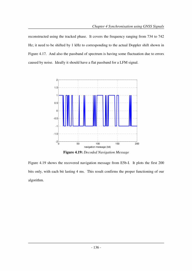
Chapter 4 Synchronisation using GNSS Signals
- 136 -
reconstructed using the tracked phase. It covers the frequency ranging from 734 to 742
Hz; it need to be shifted by 1 kHz to corresponding to the actual Doppler shift shown in
Figure 4.17. And also the passband of spectrum is having some fluctuation due to errors
caused by noise. Ideally it should have a flat passband for a LFM signal.
0 50 100 150 200-2
-1.5
-1
-0.5
0
0.5
1
1.5
2
navigation message (bit)
Figure 4.19: Decoded Navigation Message
Figure 4.19 shows the recovered navigation message from E5b-I. It plots the first 200
bits only, with each bit lasting 4 ms. This result confirms the proper functioning of our
algorithm.

Chapter 4 Synchronisation using GNSS Signals
- 137 -
Range samples
Azi
muth
posit
ion
s
50 100 150 200 250
0.5
1
1.5
2
2.5
3
3.5
x 104
(a) Range compression of heterodyne data
0 50 100 150 200 250-45
-40
-35
-30
-25
-20
-15
-10
-5
0
Range samples
Mag
nitu
de,
dB
(b) Range cross-section
0 0.5 1 1.5 2 2.5 3 3.5 4
x 104
1000
1500
2000
2500
3000
3500
4000
Azimuth positions
Magnitude
(c) Azimuth signal
10-3
10-2
10-1
100
101
-44
-42
-40
-38
-36
-34
-32
-30
Integration Time (s)
Sid
elo
be L
eve
l (d
B)
(d) the RMS sidelobe vs. the integration time
Figure 4.20: Range Compression Results

Chapter 4 Synchronisation using GNSS Signals
- 138 -
Figure 4.20 represents the correlation obtained between the proposed local reference
shown in Figure 4.12, and the input heterodyne channel signal. For these results, only
delay and frequency variation has been added to the local reference, without the phase
information. It is seen that the algorithm gives a good compensation of delay variation
and all correlation peaks are shifted to the first range bin. It confirms our tracking results
and local reference generation method. Figures 4.20(b) and 4.20(c) give the cross-section
in the range and azimuth axis for the first range bin. Figure 4.20(d) shows the RMS
sidelobe versus the integration time. The maximum integration time is the duration of the
aperture synthesis. This analysis would show that the synchronisation is valid over the
entire image formation duration. It demonstrates that the proposed algorithm is
functioning satisfactorily and good enough over the entire integration interval.
Range samples
Azi
muth
frq
ue
ncy
50 100 150 200 250
0
100
200
300
400
500
600
700
800
900
(a) FFT output

Chapter 4 Synchronisation using GNSS Signals
- 139 -
0 200 400 600 800 1000-100
-90
-80
-70
-60
-50
-40
-30
-20
-10
0
Azimuth frequency
Mag
nitu
de,
dB
(b) Azimuth cross section
730 735 740 745 746-40
-35
-30
-25
-20
-15
-10
-5
0
5
10
Azimuth frequency
Mag
nitu
de,
dB
(c) zoom view
Figure 4.21: FFT of Range Compression Results
Figure 4.21 represents the FFT output of range compression results. Figures 4.21(b) and
4.21(c) show the azimuth cross-section of the FFT output and its zoomed view. The
spectrum of azimuth signal at the first range bin is coincident with the Doppler spectrum
shown in Figure 4.18 (e). This again confirms the proper functioning of the proposed
synchronisation and range compression algorithms.
4.5 Summary
In this chapter we discussed the synchronisation issues specifically for SS-BSAR using
GNSS satellites. The synchronisation algorithm was verified using computer modelling
and experimentation. The performance of the algorithm was also analysed in terms of
varying signal dynamics and in the presence of noise.

Chapter 4 Synchronisation using GNSS Signals
- 140 -
It was pointed out that one of the key advantages of using GNSS transmitters is that it is
possible to locally generate an ideal noiseless reference signal, as the transmitted
pseudorandom noise codes are fully known. However, this is not possible when using
other transmitters of opportunities (such as ASTRA, Iridium etc), as the transmitted
information is random. The other advantage of a locally generated reference signal is
that one can reject interference from other satellites. It was suggested that for GNSS
signals the block adjustment of synchronising signal algorithm can be applied to track the
parameters, such as fine delay and Doppler variation. The proposed range compression
algorithm uses a locally generated reference signal modulated with tracked parameters,
secondary codes and navigation messages. Experimental results of the synchronisation
and range compression algorithm were presented and explained.
References
1. Willis, N.J., Bistatic Radar. 1991: Artech House.
2. Autermann, J.L., Phase stability requirements for a bistatic SAR, in IEEE
National Radar Conference. 1984. p. 48 - 52.
3. Krieger, G. and M. Younis, Impact of oscillator noise in bistatic and multistatic
SAR. Geoscience and Remote Sensing Letters, IEEE, 2006. 3(3): p. 424-428.
4. Wang, W.Q., GPS-based time and phase synchronization processing for
distributed SAR. IEEE Trans. Geosci. Remote Sens., 2009. 45(3): p. 1040-1051.
5. Nies, H., O. Loffeld, and K. Natroshvili, The bistatic aspect of the TanDEM-X
mission, in Geoscience and Remote Sensing Symposium IEEE International. 2007.
p. 631 - 634.
6. Lopez-Dekker, P., et al., Phase Synchronization and Doppler Centroid Estimation
in Fixed Receiver Bistatic SAR Systems. Geoscience and Remote Sensing, IEEE
Transactions on 2008. 46(11): p. 3459 - 3471
7. Espeter, T., et al., Synchronization techniques for the bistatic
spaceborne/airborne SAR experiment with TerraSAR-X and PAMIR, in
Geoscience and Remote Sensing Symposium, 2007. IGARSS 2007. IEEE
International 2007. p. 2160 - 2163.

Chapter 4 Synchronisation using GNSS Signals
- 141 -
8. Espeter, T., et al., Progress of Hybrid Bistatic SAR: Synchronization Experiments
and First Imaging Results, in Synthetic Aperture Radar (EUSAR), 2008 7th
European Conference on 2008. p. 1 - 4.
9. Tsui, J.B., Fundamentals of Global Positioning System Receivers: A software
Approach. 2000: John Wiley & Sons Inc.
10. Cherniakov, M., et al., Bistatic Synthetic Aperture Radar with Emitters of
Opportunity. 2006, Unversity of Birmingham: Birmingham.
11. Borre, K., et al., A Software-defined GPS and Galileo Receiver - A single-
Frequency Approach. 2007, Boston: Birkhauser.
12. Peterson, R.L., Introduction to Spread Spectrum Communications. 1995: Prentice
Hall.
13. Galileo Open Service Signal In Space Interface Control Document. 2006,
European Space Agency / Galileo Joint Undertaking.

Chapter 5 Experimental Hardware
- 142 -
Chapter 5 Experimental Hardware
5.1 Overview
To confirm system feasibility and investigate the system performance of the proposed
SS-BSAR, experimentation methodologies have been proposed and a set of experiments
have been planned and executed for real data collection. For these purposes, appropriate
radar hardware and a receiver have to be designed and built.
This chapter presents a description of the hardware involved in the SS-BSAR
experiments. The main experimental hardware is:
� Antennas and front-end, including the heterodyne channel antennas, the radar
channel antennas, an antenna for a GPS receiver, and the RF front-ends
attached to the antennas.
� A radar receiver with three receiving channels, which can be modified to receive
GLONASS L1 signals or Galileo E5a/b signals respectively.
� A data acquisition subsystem, consisting of one six-channel ADC, a sampling
clock, data acquisition card, and host PC.
� Other subsystems, including a power supply unit, two frequency synthesizers
used as a local oscillator and one commercial dual-frequency differential
GPS/GLONASS receiver to store the platform’s position information.
In the following sections, the different requirements will be analysed for the heterodyne
channel antenna and the radar channel antenna. An RF front-end design is compared

Chapter 5 Experimental Hardware
- 143 -
with different arrangements. It is suggested that the architecture of the radar receiver
uses two stage down-conversion to collect complex data with in-phase and quadrature (I-
Q) channels. In order to maximise the dynamic range of the ADC the total required gain
for the amplification chain is calculated based on Galileo E5 signal reception. The
impact of the quantization scheme and the sampling frequency will also be discussed; and
different hardware testing set-ups will be introduced and discussed in section 5.3 with
extensive testing results included in the Appendix.
5.2 Experimental Hardware Development
5.2.1 Antennas and Front-end
For the proposed SS-BSAR system, two receiving channels will be used, for the direct
signal synchronisation and the reflected signal imaging. Two antennas will be required,
as one looks at the sky and the other one points to the ground target area. There are
different requirements for these antennas due to the different purposes.
First of all, a right-hand circularly polarized (RHCP) antenna will be used in the
heterodyne channel (receiving a direct GNSS signal) and a left-hand circularly polarized
(LHCP) antenna will be used in the radar channel (receiving a reflected signal from the
target area) to decrease the level of direct path interference from the satellite. This is
because all GNSS satellites are using a right-hand circularly polarized antenna for
navigation signals transmission.
Chapter 5 Experimental Hardware
- 144 -
Ideally, the heterodyne antenna should cover a wide spatial angle to receive the
maximum number of signals. The suggested requirement is to receive signals from all
GNSS satellites about 10 degrees above the horizon. The reason behind this is to have
the flexibility to form the optimal bi-static/multi-static topology and the capability for
advance SAR applications, such as single pass interferometry and radiogrammetric 3-D
surface mapping. Furthermore, the antenna should have a uniform gain over this very
wide spatial angle. If an antenna has a large gain variation from zenith to azimuth, the
strength of the received signals will not be consistent. In a CDMA system like GNSS, it
is desirable to have comparable signal strength from all the received signals. Otherwise,
the strong signals may interfere with the weak ones and make it difficult to detect them.
Also, the heterodyne channel antenna should reject or minimise the multipath effect. It is
caused by reflecting from the ground, or buildings, that add to the direct path signal. The
reflection of a right-hand circularly polarized signal is a left-hand circularly polarized
signal. A right-hand circularly polarized receiving antenna has a higher gain of the
signals received from the satellites, and a lower gain for the reflected signals because the
polarization is in the opposite direction. One common multipath effect is the reflection
from the ground below the antenna. Therefore, an ideal heterodyne channel antenna
should have a low back lobe. Some techniques such as a specially designed ground plane
can be used to minimise the multipath from the ground below.
For the radar channel antenna in the SS-BSAR, its selection is mainly dependent on the
platform restriction and the imaging requirements. Its beamwidth is decided by the SAR
operation mode and the size of the target area. It could be a wide beamwidth antenna

Chapter 5 Experimental Hardware
- 145 -
covering the whole imaging area or a narrow beamwidth antenna for a strip-map SAR
mode. Both mechanically steered antennas and electronic phase arrays can be used
depending on the platform and other requirements. Its gain will then be limited by its
size and beamwidth. One thing to notice is that there is no need for antenna footprint
synchronisation between the transmitting antenna on the GNSS satellite and the
receiver’s radar channel antenna. It is simply because all GNSS signals are transmitted
by the global beam and cover the entire part of the earth’s surface that is visible to the
satellite.
(a) Antennas: patch antenna, helix antenna,
GNSS antenna
(b) RF front-end
(c) Flat PCB patch design
(d) Heterodyne channel antenna

Chapter 5 Experimental Hardware
- 146 -
(e) Four element antenna array (radar channel antenna)
Figure 5.1: Antennas and RF Front-end
One common antenna design to receive a circular polarized signal is a spiral helix
antenna, which inherently has a wide bandwidth. Another popular design is a microstrip
antenna, which is sometimes referred to as a patch antenna. The advantage of the patch
antenna is its simplicity and small size. Figure 5.1 displays the antenna selected and
designed for the SS-BSAR using GNSS experiments, and Table 5.1 below gives its main
parameters. More specifications can be found for the displayed antennas in Appendix C,
and the application of these antennas will be discussed in Chapter 6 together with the
experimental set-up description.
Table 5-1: Antenna Parameters
Antenna Gain (dBi) Beamwidth
Spiral helix antenna 16 30ох30
о
Flat PCB patch antenna 9 65ох66
о
GPS antenna 6 Omni-directional
Patch antenna array 14 65ох15
о
In this chapter, an RF front-end refers to the first block connecting between the antenna
and the long cable to the receiver. It can have one, or two, low noise amplifier (LNA)
stages and one bandpass filter. There are many different ways to build an RF front-end.

Chapter 5 Experimental Hardware
- 147 -
The two important factors concerned are the total gain and filter installation. The first
component following the antenna can be either a filter or an amplifier. Both
arrangements have advantages and disadvantages. If the antenna is integrated with an
amplifier, the first component after the antenna is the amplifier. Bandpass filters can be
connected first and used to reject out-of-band signals and limit the noise bandwidth, but
they would add insertion loss. If I-Q channels are used, filters may increase the difficulty
of amplitude and phase balancing.
In general, the noise figure of a receiver can be expressed as (similar to noise temperature
shown in equation 2.12)
2 21
1 1 2 1 2
11 1 N
N
FF FF F
G G G G G G
−− −= + + + +�
�
(5.1)
where NF and NG (i=1,2, …N) are the noise figure and gain of each individual
component in the RF chain. If the amplifier is the first component, the noise figure of the
receiver is low and is approximately equal to the noise figure of the first amplifier, which
can be less than 2 dB. The potential problem with this approach is that strong signals in
the bandwidth of the amplifier may drive it into saturation and generate spurious
frequencies. If the first component is a filter, it can stop out-of-band signals from
entering the input of the amplifier. However, the insertion loss of a narrowband filter is
usually relatively high, about 2-3 dB. The received noise figure will be about 2-3 dB
higher than the previous arrangement.

Chapter 5 Experimental Hardware
- 148 -
For the RF front-end design shown in Figure 5.1 (b), it has a first stage LNA (AM50-
0002, 1.15 dB noise figure with 27 dB gain), followed by a RF bandpass filter (centre
frequency at 1191 MHz with 51 MHz bandwidth for Galileo E5 reception) and a second
stage RF amplifier with 15 dB gain. Its testing results and the datasheet for each
component can be found in Appendix C.
5.2.2 Experimental Radar Receiver
The external views for the experimental hardware are shown in the figure below. All
hardware and subsystems are installed into three standard 19-inch racks within one flight
case. The top rack hosts the data acquisition subsystem with an output interface to a PC,
the middle one is the microwave receiver, and the GPS receiver and other subsystem is
inside the bottom rack. In the following sections, the block diagram of each rack will be
provided and a description of it will be given.

Chapter 5 Experimental Hardware
- 149 -
(a) Front view, inputs to three receiving
channels and data interface to PC
(b) Rear view, three pairs I/Q outputs and
other inter-connection ports
(c) Rear view with all ports connected
(d) Fully connected microwave receiver
with a laptop for data collection
Figure 5.2: Experimental Radar Receiver
The function of a radar receiver is to amplify the radar echoes and to filter them in a
manner that will provide the maximum discrimination between the desired echoes and
undesired noise and interference. This microwave receiver (Figure 5.3) consists of three
identical receiving channels: the heterodyne channel (HC), the radar channel (RC) and
the spare channel (SC). A power supply and local oscillator interface is also included.
The third channel (SC) is a backup and will be brought into use while conducting the
interferometry experiment.

Chapter 5 Experimental Hardware
- 150 -
The proposed design for the microwave receiver is a two-stage down-conversion, as
mentioned earlier. All three channels are designed to receive the Galileo E5 signal and
convert it to baseband in-phase (I) and quadrature (Q) outputs. However, these channels
could be modified to receive the GLONASS L1 signal as well. Details of this can be
found in document [1].
Figure 5.3: Photo of Microwave Receiver
Each receiving channel of the microwave receiver is divided into three parts (block
diagram shown in Figure 5.4): the radio frequency (RF) part, centred on the E5 carrier
frequency 1191.795 MHz, intermediate frequency (IF) part, centred on 140 MHz, and the
baseband part with 10 MHz bandwidth. See Appendix G for a list of all the components
used and the specifications.

Chapter 5 Experimental Hardware
- 151 -
Figure 5.4: Microwave Receiver Block Diagram
The RF part includes a low noise amplifier (LNA1, the same as the one used in the front-
end) connected to the front-end and the antenna through a coaxial cable, and a band-pass
filter (BPF1), to suppress the strong interference from adjacent-frequency satellites. The
IF part consists of a 140 MHz band pass filter (BPF2), four cascaded IF amplifiers (A1-
A4) with a total estimated gain of 100 dB, and a 10 dB attenuator between the 3rd
and 4th
IF amplifier to avoid the last amplifier entering into the saturation and to improve the
impedance matching between the components. The baseband part has an I/Q
demodulator and two low pass filters (LPF1).
The received signal, after the initial RF amplification, is shifted to an intermediate
frequency by mixing with a local-oscillator (LO1) frequency. Most amplification (~100

Chapter 5 Experimental Hardware
- 152 -
dB gain) will be applied at the IF stage. Not only is amplification at IF less costly and
more stable than at microwave frequency, but also the wider percentage bandwidth
occupied by the desired signal simplifies the filtering operation. In addition, the receiver
can vary the LO1 frequency to follow any desired tuning variation of the transmitter
without disturbing the filtering at IF. Ideal mixers in a receiver act as multipliers, which
produce an output that is proportional to the product of the two input signals. Except for
the effect of nonlinearity and unbalance, these mixers only produce two output
frequencies, which are equal to the sum and the difference of the two input frequencies.
After IF stage amplification and filtering, the IF signal is applied to a splitter and
the resulting signals are mixed with two local oscillator (LO2) signals that are 90º apart in
the phase. This process produces in-phase and quadrature output signals. After a low
pass filter, the signal will be digitized and transferred to the computer hard disk through
the data acquisition subsystem. Figure 5.5 shows the block diagram of the full receiving
chain for two channels. It can be seen that two local oscillators, LO1 and LO2 are phase
locked with the common frequency reference. This is critical for maintaining the
coherence between the heterodyne channel signal and the radar channel signal.

Chapter 5 Experimental Hardware
153
A1 A2 A3 A4
LNA1 A1 A2 A3 A4
BPF2
BPF2BPF1
M1
M1
A5
I/QDemodulator
I/QDemodulator
Splitter0
0Splitter
00
LPF1
LPF1
LPF1
LPF1
Locked to Common Clock
Splitter00
Splitter900
M2
M2
+7dBm
+7dBm
+10dBmS1 S2
0 dBm
Local Oscil+20dBm
+17dBm
+17dBm
S3IF
S4
I/Q Demodulator
HCAntenna
RCAntenna
I
Q
I
Q
RF Part IF Part Baseband Part
LO1 (1.347GHz)
LO1 (140MHz)
To PC Storage
To PC Storage
10 dB
10 dBTo PC
Storage
To PC Storage
Attenuator
Attenuator
LNA1 BPF1
Figure 5.5: Microwave Receiver Receiving Chain (2 channels shown)

Chapter 5 Experimental Hardware
- 154 -
In this section the signal level and the required amplification will be discussed. The E5
signal level at the input of the front-end should be at least -155 dBW (-125 dBm), as
discussed in Chapter 2. The available thermal noise power at the input of a receiver is
i sN kT B= (5.2)
where k is the Boltzmann’s constant, sT is the temperature in Kelvin, B is the
bandwidth of the receiver noise in hertz, and iN is the noise power in watts. The thermal
noise at room temperature where Ts=290 K expressed in dBm is -114 dBm/MHz
( 1010 log ( )skT× , dBW/Hz).
For the heterodyne channel, the input to the receiver is an antenna pointing at the sky; the
thermal noise is lower than room temperature, such as 50 K.
For the E5a or E5b signal, the null-to-null bandwidth is about 20.46 MHz. But the BPF1
(indicated in Figure 5.5) has a bandwidth of 51 MHz and in order for it to have the
capability of receiving the full E5 (E5a and E5b) signal, the noise figure of LNA1 is 1.15
dB. Thus, the noise floor of the microwave receiver is at -97 dBm approximately.
Supposing that the E5 signal is at -125 dBm at the input of RF front-end, the signal is 28
dB below the noise floor. One cannot expect to see the signal directly in the collected
data.
The amplification needed depends on the analogue-to-digital converter (ADC) used to
digitize the I-Q outputs. A simple rule is to amplify the signal to the maximum range of
the ADC. However, this approach should not be applied to the GNSS signal, because the

Chapter 5 Experimental Hardware
- 155 -
signal is below the noise floor. If the signal level is brought to the maximum range of the
ADC, the noise floor will saturate the ADC. Therefore, in this design the noise floor,
rather than the signal level, should be raised close to the maximum range of the ADC.
The maximum voltage to exercise the level of the ADC is about 3.8 V (LT1715) and the
corresponding power is
23.80.2888 24.6
50P watt dBm= = = (5.3)
It is assumed that the system has a characteristic impedance of 50 ohm. A simple way to
estimate the gain of the amplifier chain is to amplify the noise floor to this level; thus, a
net gain of about 122 dB (24.6+97) is needed. Since in the RF chain there are filters,
mixer, and cable loss, the insertion loss of these components must be compensated with
additional gain. The net gain must be very close to the desired value of 122 dB. Too low
a gain value will not activate all the possible levels of the ADC. Too high a gain will
saturate some components of the ADC and create an adverse effect.
For the receiving channel in Figure 5.5, the total amplification gain is 123 dB with 30 dB
loss from mixers, filters and the attenuator. So the net gain is around 93 dB. However,
with a 41 dB gain from front-end directly attached to the antenna, the total net gain is
around 134 dB for the whole receiving chain. Please note that the calculation here does
not include any cable loss, particularly the long cable used to connect the antenna with
the receiver. The actual output level of the microwave receiver is around 700-800 mV
which is enough to exercise the selected ADC.

Chapter 5 Experimental Hardware
- 156 -
There is one disadvantage that should be noted. For the I-Q demodulator, the 90-degree
phase shift is introduced in the oscillator block. For a wide band receiver, the I-Q
approach can double the input bandwidth with the same sampling frequency. However,
the amplitude and phase of the two outputs are difficult to balance accurately, and the
phase history of the input signal is vital for SAR image formation and needs to be
measured accurately.
5.2.3 Data Acquisition Subsystem
Through the microwave receiver, the input signal is down converted into I-Q channels.
The data collected through this approach are complex and the two sets of data are often
referred to as real and imaginary. Since there are two channels, the Nyquist sampling is
equal to the bandwidth of the input signal.
As discussed previously, the Galileo E5 signal is a CDMA signal. The dynamic range of
a Galileo receiver need not be very high. An ADC with a few bits is relatively easy to
fabricate and may operate at a high frequency. Another advantage of using fewer bits is
that it is easier to process the digitized data. The disadvantage of using fewer bits is the
degradation of the SNR. Spilker [2] indicated that 1-bit ADC degrades the SNR by
1.96 dB and a 2-bit ADC degrades the SNR by 0.55 dB. Chang [3] claims that the
degradation is due to the number of bits of the ADC and is a function of input SNR and
sampling frequency. A low SNR signal sampled at a higher frequency causes less
degradation in a receiver. The GNSS signal should belong to the low SNR case because
the signal is below the noise. At a Nyquist sampling rate, the minimum degradation is

Chapter 5 Experimental Hardware
- 157 -
about 3.01 dB and 0.72 dB for 1- and 2- bit quantizers, respectively. At five times the
Nyquist sampling rate, the minimum degradation is 2.18 dB and 0.6 dB for 1- and 2- bit
quantizers, respectively.
Although the sampling frequency discussed in this chapter is given a pre-defined
mathematical value, the actual frequency used in the hardware usually has limited
accuracy. The most important effect of sampling frequency inaccuracy may be the error
in the pseudorange (fine code delay) measured, which has been discussed in section 4.3.
For the experimental hardware, the 1-bit quantization scheme is proposed. The purpose
built data acquisition subsystem includes three components: an ADC board with six
channels, one commercially available data acquisition card and a sampling clock. The
ADC board first converts the analogue signal to a digital signal that can be accepted as
the input of the data acquisition card. Due to the character of the received analogue
signal, which is a pseudo-random sequence buried in noise, it is adequate to divide the
voltage range of the signal into two discrete levels and to store it as a binary signal. The
serial digital signal is subsequently sampled at a clock rate specified either by an on-
board oscillator clock or by an external clock. For our experiments a sampling clock of
50 MHz is used in order to over-sample the Galileo E5a/b signal by a factor of ~5. A
higher sampling rate could be used but it would need a high performance ADC and would
increase the computation of signal processing significantly. Sampled digits are then
transferred to the memory of the data acquisition card using a continuous FIFO mode.

Chapter 5 Experimental Hardware
- 158 -
Finally, using the appropriate software, this data stream is recorded on the computer hard
disk for further processing. See Appendix E for further detail about this process.
Figure 5.6: Photo of Data Acquisition Subsystem
Figure 5.6 above shows the contents of rack holding the data acquisition subsystem.
Figure 5.7 below gives its block diagram. A 10 MHz frequency reference is taken out
from the sampling clock and used to lock two local oscillators. Hence, the microwave
receiver has one common reference, which is an OCXO with a frequency stability of
± 0.5 ppm. It is equal to the frequency accuracy of ±25 Hz for 50 MHz output.

Chapter 5 Experimental Hardware
- 159 -
ADC Sampling
Clock
Docking Station with Data
Acquisition Card
Raw data
input
Clock
input
Sampled
data
To computer for data storage /
Express Card Interface
Ref
I/O
Power in
+12 V
+5 V
+12 V
Ref
I/O
Output
I
O
Figure 5.7: Block Diagram of Data Acquisition Subsystem
5.2.4 Other Receiver Subsystems
Figure 5.8: Photo of Other Receiver Subsystems

Chapter 5 Experimental Hardware
- 160 -
Figure 5.8 above shows the contents of bottom rack, which includes a commercial
GLONASS/GPS receiver; two frequency synthesizers and power supply units.
GPS
ReceiverFrequency
Synthesizer
Frequency
Synthesizer
SDC-DC Converters
28-12 V, 12-15 V,
12-5 V
Backup
Battery
12 V
Ref
I/O
Ref
I/O
Ref
I/O
RF
in
Data
out
LO1 LO2
28/12 V
DC IN12 V
OUT
12 V
OUT
5 V
OUT
+12
V
+5/+15 V +5 V
To receiver To receiver
Figure 5.9: Block Diagram of Other Receiver Subsystems
Figure 5.9 above gives the block diagram. More details about the hardware in this block
can be found in Appendices D and F.
5.3 Experimental Hardware Testing
To ensure proper operation and the collection of good data, all hardware had to be fully
tested in the laboratory environment to prove its functionality. A set of testing set-ups
will be discussed for antennas, the data acquisition subsystem and the microwave receiver
respectively in this section.

Chapter 5 Experimental Hardware
- 161 -
5.3.1 Antenna Testing
Ideally the antenna radiation pattern should be measured in an anechoic chamber.
However, due to the lack of availability of an anechoic chamber, a set of experiments
have been performed in an open space to measure the gain and the beamwidth of the
heterodyne and radar channel antennas. Figure 5.10 below shows the experimental set-up
for antenna testing.
Figure 5.10: Heterodyne Channel Antenna Testing Set-up
For heterodyne channel antenna gain, S21 measurements have been made using a
network analyser. Two identical patch antennas were installed with a separation distance
of 7 metres, one for transmission and the other for reception. The network analyser
calibration was carried out first and the input power level was adjusted to set the
measured total transmission link gain (propagation loss, antenna gain, losses from cables
etc.) to 0 dB.

Chapter 5 Experimental Hardware
- 162 -
For the radar channel antenna (4-element array) testing, an additional one-element patch
antenna was used for transmission, with the antenna array being used for reception. The
phase centres of the two antennas were set to the same height with a separation distance
of 8 m. The antenna gain and beamwidth were found by rotating one antenna and taking
the maximum and 3 dB readings of the received signal power from the spectrum analyser.
The approximate beamwidth was then derived from the angle between the two 3 dB
readings.
Figure 5.11: Radar Channel Antenna Testing Set-up
The testing results are included in Appendix C.
5.3.2 Data Acquisition Subsystem Testing
The data acquisition subsystem test consisted of testing the ADC board and the data
acquisition card separately. The assembled subsystem was then tested with a sine wave
and a square wave as inputs. The stored data was used to reconstruct the input signal

Chapter 5 Experimental Hardware
- 163 -
with MATLAB, allowing checks of the working frequency range and the lowest
permissible input amplitude of the subsystem.
Figure 5.12 below shows a simplified test set-up. Preliminary tests start with a test of the
ADC only. A 50 MHz signal generated using the satellite imitator is fed directly into the
ADC and shown on the oscilloscope. A common clock is used to synchronize the
satellite imitator and the sampling clock. Various signal levels have been generated to
check the range of input voltages for the ADC.
Figure 5.12: ADC Test Arrangement
Figure 5.13 below shows the testing setup for the whole data acquisition subsystem.
With a baseband 10 MHz PRN sequence generated by an AMIQ generator, this analogue
input signal has been converted to digital bits, sampled by the data acquisition card with a
50 MHz clock, and written into files on the hard disk. The stored data has then been
divided into multiple files for each channel and the correlation with a locally generated
PRN code has been used for a data integrity check.

Chapter 5 Experimental Hardware
- 164 -
The results for these two testing set-ups are included in Appendix E.
Figure 5.13: Data Acquisition Subsystem Test Arrangement
From the tests, we know that the internal interference of the ADC board and the
impedance mismatch between the output of the ADC and the input of the PCI card are the
potential sources of system degradation on bit error rate. Transmission line effects and
environment noise, particularly on the clock and control lines, also require attention. It is
advisable to use twisted-pair connections to the data acquisition card, each digital I/O
signal line being twisted with a GND line, and to place a shield around the wires.
5.3.3 Experimental Microwave Receiver Testing
To ensure the full functioning of the assembled microwave receiver, the testing process is
started from individual components, to connected blocks, and to the full receiving chain
with noise and signals at the input. The testing mainly includes:

Chapter 5 Experimental Hardware
- 165 -
� RF parts testing: LNA and BPF
� IF parts testing: mixer, amplifier, BPF
� Baseband parts testing: splitter, mixer, BPF
� Test with noise – see noise RMS level on the oscilloscope
� Test with noise – record noise, investigate ACF and CCF
� Test with signals – see signal level (reduced gain scenario) on the oscilloscope
� Test with signals - record signal, investigate ACF, CCF
Figure 5.14: Microwave Receiver Noise Testing
Figure 5.14 above shows the diagram for receiver noise testing. No input signal will be
applied and only a 50 ohm load is connected at the RF input of the microwave receiver.
Only the receiver noise will appear at the input of the data acquisition subsystem and will
be sampled and stored into the host PC.

Chapter 5 Experimental Hardware
- 166 -
Microwave
ReceiverADC
Host
PC
receiving channel
receiving channel
SplitterSatellite
imitator
Common
clock
Figure 5.15: Microwave Receiver Simplified Testing Arrangement
Figure 5.15 shows a test set-up including the microwave receiver. A locally generated
signal with 1191.795 MHz centre frequency and 10 MHz bandwidth will be applied at the
RF input of microwave receiver. This is split and fed into the separate channels of the
microwave receiver. Both the receiver noise and signal output will appear at the input of
the data acquisition subsystem and will be sampled and stored into the host PC. The
input signal level is set to higher than the nominal received Galileo E5 signal level as no
front-end is used. A common clock is used to synchronize the transmitter and the
receiver. Checking the stored data will verify the working of the microwave receiver.
MicrowaveReceiver
ADCHostPC
low-gain channel
high-gain channel
SplitterSatellite imitator
Common clock
LNA1 BPF1 LNA2
LNA1
Attenuator
Figure 5.16: Microwave Receiver Full Channel Testing Arrangement

Chapter 5 Experimental Hardware
- 167 -
Figure 5.16 shows a full experimental testing arrangement, including all the components
to be used in the outdoor experiments. A locally generated RF Galileo E5 signal is split,
one copy going into a high-gain receiver channel (the radar channel) and the other going
into the low-gain receiving channel (the heterodyne channel, with the gain reduced for
testing purposes). The front-end is used with a high-gain channel and one low-noise
amplifier LNA1 is used with the low-gain channel to compensate for the loss within the
coaxial cables, which connect the satellite imitator and microwave receiver. The input
signal level is set to the same as the nominal received Galileo E5 signal level. The full
set of testing results are included and analysed in Appendix G.
5.4 Summary
This chapter discusses the development and testing of the hardware and the receiver
involved in the SS-BSAR experiments. The heterodyne channel antenna should have a
broad beam to receive signals from the zenith to the horizon. It should be right-hand
circular polarized to reduce the reflected signals. The overall gain of the amplifier chain
depends on the input voltage of the ADC. The overall gain is about 120 dB to receive
Galileo E5 with the proposed hardware. The input signal is suggested to be down
converted to baseband and then digitized, because it is simpler to build than direct
digitization. The number of quantization bits is discussed, and one or two bits may be
enough for GNSS signal recovery with a small degradation of receiver sensitivity. The
impact of sampling frequency accuracy is also discussed. Finally, several experimental
testing setups are presented to confirm the functionality of the designed hardware and

Chapter 5 Experimental Hardware
- 168 -
receiver. Further details on hardware specifications and the testing results are included in
Appendices C-G.
Reference
1. Cherniakov, M., et al., Bistatic Synthetic Aperture Radar with Emitters of
Opportunity. 2006, Unversity of Birmingham: Birmingham.
2. Spilker, J.J.J., Digital communication by satellite. 1995, Englewood Cliffs:
Prentice Hall.
3. Chang, H., Presampling filtering, sampling and quantization effects on the digital
matched filter performance, in International Telemetering Confrerence. 1982:
San Diego, CA. p. 889-915.

Chapter 6 Experimentations and Parameters Estimation
- 169 -
Chapter 6 Experimentations and Parameters Estimation
6.1 Overview
This chapter consists of two main parts. The first part introduces the programme of
experimentation, which leads to the ultimate objective of airborne SS-BSAR imaging.
Experiment strategies and trials plans are designed to investigate the system feasibility of
SS-BSAR using GNSS as a non-cooperative transmitter. The results from these
experiments will establish potential system performance and allow the identification of
possible applications for SS-BSAR.
Figure 6.1: Experimentation Methodology
Figure 6.1 gives the overall experimentation methodology; it includes three stages:
stationary receiver, ground moving receiver and airborne receiver. The program of work
starts with the stationary receiver experiments and subsequent experiments with the
receiver mounted on the ground vehicle and then an airborne moving platform. It has
been established that when, in BSAR, both the transmitter and the receiver are in motion
along their own trajectories. These two independent trajectories and associated speed
vectors can be replaced with one effective trajectory and speed vector that characterize

Chapter 6 Experimentations and Parameters Estimation
- 170 -
the resolution ability of the system. This is an important conclusion that allows us to start
experimentation with only the transmitter moving.
Figure 6.2: Experimental Set-up for Imaging Data Collection
Figure 6.2 presents the common experimental set-up using the hardware described in
Chapter 5 for data collection. In addition to the radar channel, the receiver includes a
navigation channel and a heterodyne channel, which uses an omni-directional antenna
pointing at the satellite to receive the Galileo E5a/b signal directly. It allows generation
of a synchronized local reference for correlation with echoes reflected from the target
area. For the experiments with satellites, the first two Galileo testing satellites, GIVOE
A/B have been used as the non-cooperative transmitter. Table 6-1 gives the parameters
of one typical ranging signal; the relevant PRN code provides 10.23 MHz bandwidth and
hence a range resolution of ~ 15 m (quasi-monostatic case).

Chapter 6 Experimentations and Parameters Estimation
- 171 -
Table 6-1: Ranging Signal Parameters
Galileo E5b-Q Ranging signal
Primary Code (1 ms long)
Carrier frequency 1207.14 MHz
Wavelength 0.2485 m
Chip rate 10.23 MHz
Received power 14 23.99 10 /W m−×
The comprehensive experimental methodologies are described and discussed in sections
6.2 to 6.4, for each stage of the experiments. The actual experimental parameters and set-
up block diagrams are also given. The potential resolution and signal-to-noise ratio for
each experiment will be calculated. Experiment topologies involving a Galileo satellite
are divided into quasi-monostatic SAR and bistatic SAR. A corner reflector (CR) has
been built as the reference target; a number of houses within the target area will also be
considered as radar targets. Separation of these reflectors will demonstrate the resolution
ability of the radar and the signal-to-noise ratio obtained with corner reflectors having
known radar cross-section may be used for power budget analysis.
The second part (section 6.5) discusses the parameter estimation problem for SS-BSAR
using GNSS. Before applying the image formation algorithm to the experimental data,
the parameters, such as the transmitter/receiver trajectories, Doppler shift and phase
histories need to be estimated with pre-defined accuracy. Practical methods are proposed
and compared for the transmitter/receiver parameter extraction and estimation. Two

Chapter 6 Experimentations and Parameters Estimation
- 172 -
specific problems, residual Doppler shift and motion compensation are briefly discussed.
The parameter estimation results from the real experimental data are presented and
discussed at the end of this chapter.
6.2 Stationary Receiver Experiments
6.2.1 Experiment Design
With the successful synchronisation experiments (discussed in Chapter 4), the proposed
synchronisation algorithm has been verified. The SS-BSAR imaging experiments can be
started. As the experimentation methodology indicated, the first stage is the experiment
with stationary receiver and moving satellite. Only satellite motion will contribute the
synthetic aperture. The main objective of this stage is to confirm the functionality of the
full hardware system, including all antennas and receiving channels. Preliminary testing
of the image formation algorithm will be carried out with the data collected, such as
range compression and azimuth reference design. To be able to use a relative simple
BSAR focusing algorithm, the quasi-monostatic topology is preferred for the stationary
receiver experiment.
Figure 6.3 shows the layout of the experimental set-up in the quasi-monostatic SAR
configuration. The quasi-monostatic SAR experiment, with a small bistatic angle, is an
important stage leading to a more general study of the range resolution and cross-range
resolution of bistatic SAR. The arrangement has three sections: the satellite, the
receiving system and the observation area. As noted previously, the receiving system

Chapter 6 Experimentations and Parameters Estimation
- 173 -
comprises of a radar receiver having a radar channel and a heterodyne channel. Both
channels’ antennas are installed on the stationary platform, with one looking at the target
area and one receiving the direct satellite signal. The preferred satellite position is at the
relatively low elevation angle and on the extended line of target-to-receiver direction, in
order to reduce the bistatic angle.
~180o
20m10m
elevation
Figure 6.3: Data Collection Geometry for Small Bistatic Angle
In the observation area corner reflectors with different radar cross-sections are positioned
at the different ranges to the receiver, separated by a range distance of 10-15 m to act as
detectable targets. The purpose of these targets is to demonstrate the range resolution
ability of the quasi-monostatic SAR, to calibrate the system power budget and to verify
the correctness of the image formation algorithm. The corner reflector should have a
sufficiently large radar cross-section, so that its range history and Doppler spectrum are
visible during the image formation processing. Due to the low power density of the
Galileo satellites on the earth, it is practically impossible to build a reflector which is
strong enough to be seen at the output of the receiver hardware.

Chapter 6 Experimentations and Parameters Estimation
- 174 -
However, this reflector may possibly be detected after range compression, especially if it
is situated close to the receiver (the transmitter’s power density on the earth’s surface can
be assumed constant). Equation 6.1 can provide a measure of the target radar cross-
section required over a particular integration time to give a sufficiently high SNR at the
output of the range matched filter.
( )2
22
int
4
λ
πσ
RD
sRRp
GP
kTR
T
SNR×=
(6.1)
Figure 6.4 shows the radar cross-section required to achieve a SNR of 13 dB at different
receiver-to-target ranges. It can be seen that for a 1 ms integration time, a 2500 m2 RCS
corner reflector 100 m away from the receiver will provide 12 dB SNR. The calculation
parameters are shown in Table 6.2 below.
Table 6-2: Calculation Parameters
Parameter Symbol Value
Receiver-to-target range RR
100-400 m
Receiver noise temperature sT
410 Kelvin
Gain of receiving antenna RG
16 dBi
Required SNR RpSNR
13 dB
Integration time intT
1 ms
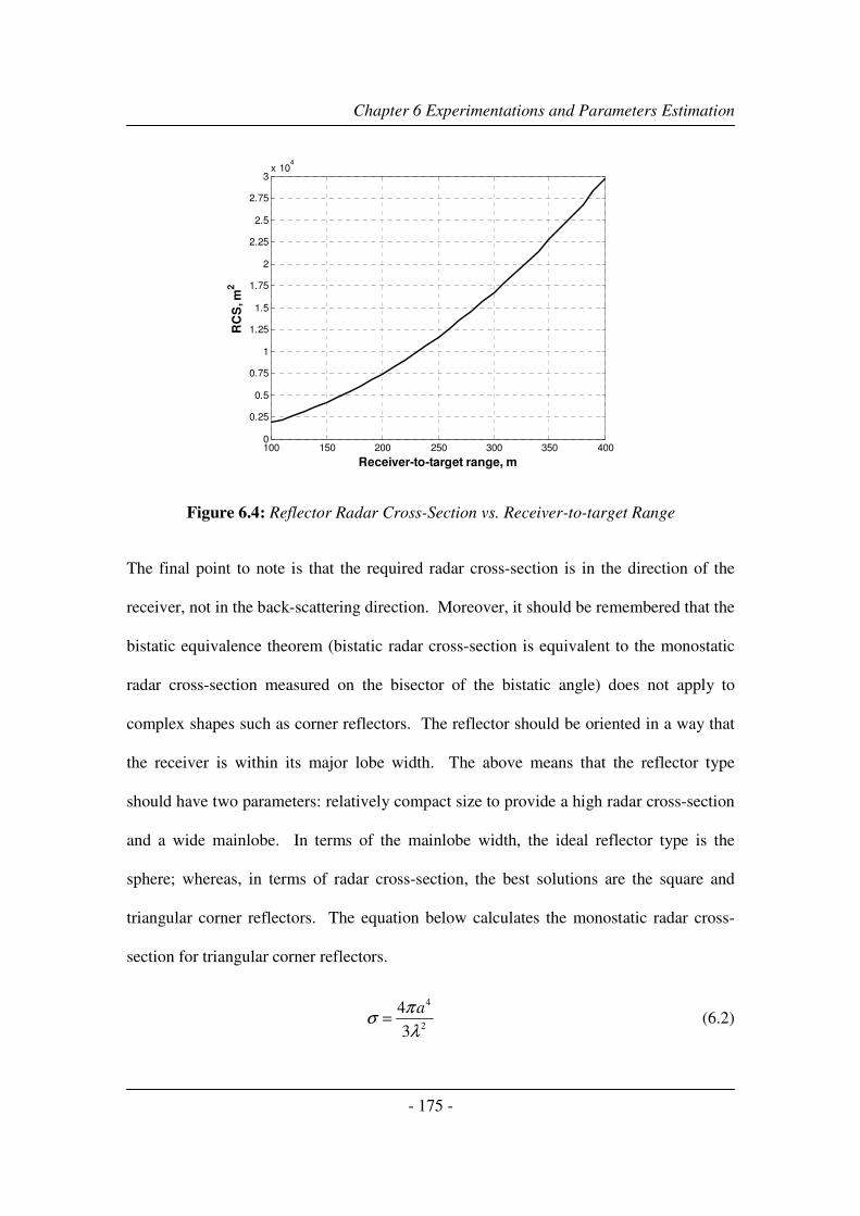
Chapter 6 Experimentations and Parameters Estimation
- 175 -
Figure 6.4: Reflector Radar Cross-Section vs. Receiver-to-target Range
The final point to note is that the required radar cross-section is in the direction of the
receiver, not in the back-scattering direction. Moreover, it should be remembered that the
bistatic equivalence theorem (bistatic radar cross-section is equivalent to the monostatic
radar cross-section measured on the bisector of the bistatic angle) does not apply to
complex shapes such as corner reflectors. The reflector should be oriented in a way that
the receiver is within its major lobe width. The above means that the reflector type
should have two parameters: relatively compact size to provide a high radar cross-section
and a wide mainlobe. In terms of the mainlobe width, the ideal reflector type is the
sphere; whereas, in terms of radar cross-section, the best solutions are the square and
triangular corner reflectors. The equation below calculates the monostatic radar cross-
section for triangular corner reflectors.
4
2
4
3
aπσ
λ= (6.2)
100 150 200 250 300 350 4000
0.25
0.5
0.75
1
1.25
1.5
1.75
2
2.25
2.5
2.75
3x 10
4
Receiver-to-target range, m
RC
S, m
2

Chapter 6 Experimentations and Parameters Estimation
- 176 -
where a is the characteristic dimension of the object. For the triangular corner reflectors,
a is the length of its vertical side.
6.2.2 Imaging Data Collection
(a) Operation space
(b) Antenna installation
Figure 6.5: Hardware Vehicle Installation
(a) Stationary receiver experiment (site 1)
(b) Reference target – corner reflector
Figure 6.6: Stationary Receiver – Reference Target
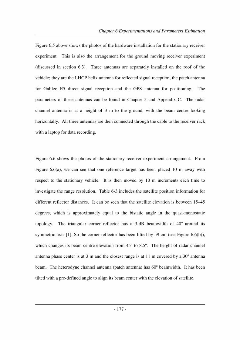
Chapter 6 Experimentations and Parameters Estimation
- 177 -
Figure 6.5 above shows the photos of the hardware installation for the stationary receiver
experiment. This is also the arrangement for the ground moving receiver experiment
(discussed in section 6.3). Three antennas are separately installed on the roof of the
vehicle; they are the LHCP helix antenna for reflected signal reception, the patch antenna
for Galileo E5 direct signal reception and the GPS antenna for positioning. The
parameters of these antennas can be found in Chapter 5 and Appendix C. The radar
channel antenna is at a height of 3 m to the ground, with the beam centre looking
horizontally. All three antennas are then connected through the cable to the receiver rack
with a laptop for data recording.
Figure 6.6 shows the photos of the stationary receiver experiment arrangement. From
Figure 6.6(a), we can see that one reference target has been placed 10 m away with
respect to the stationary vehicle. It is then moved by 10 m increments each time to
investigate the range resolution. Table 6-3 includes the satellite position information for
different reflector distances. It can be seen that the satellite elevation is between 15–45
degrees, which is approximately equal to the bistatic angle in the quasi-monostatic
topology. The triangular corner reflector has a 3-dB beamwidth of 40º around its
symmetric axis [1]. So the corner reflector has been lifted by 59 cm (see Figure 6.6(b)),
which changes its beam centre elevation from 45º to 8.5º. The height of radar channel
antenna phase center is at 3 m and the closest range is at 11 m covered by a 30º antenna
beam. The heterodyne channel antenna (patch antenna) has 60º beamwidth. It has been
tilted with a pre-defined angle to align its beam center with the elevation of satellite.

Chapter 6 Experimentations and Parameters Estimation
- 178 -
Table 6-3: Satellite Positions and Reflector Distance
Distance Elevation Azimuth
10 m 34 52
20 m 32 53
30 m 16 54
45 m (site 2) 45 84
The azimuth and elevation angles of the satellite are measured with respect to the
heterodyne antenna; however, it can be assumed that these measurements are the same as
measurements made with respect to the corner reflector, due to the close proximity of the
reference locations. The experimental imaging results are discussed in section 7.2 from
two collected data sets.
Figure 6.7: Stationary Imaging – Site 2
Receiver
Reference
target
Satellite
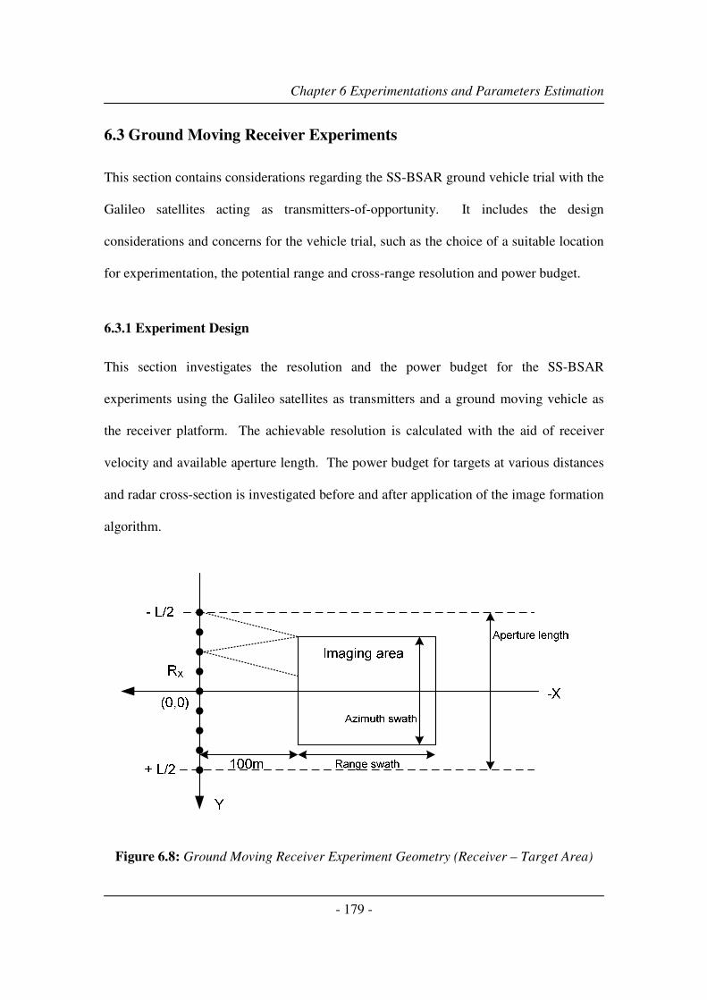
Chapter 6 Experimentations and Parameters Estimation
- 179 -
6.3 Ground Moving Receiver Experiments
This section contains considerations regarding the SS-BSAR ground vehicle trial with the
Galileo satellites acting as transmitters-of-opportunity. It includes the design
considerations and concerns for the vehicle trial, such as the choice of a suitable location
for experimentation, the potential range and cross-range resolution and power budget.
6.3.1 Experiment Design
This section investigates the resolution and the power budget for the SS-BSAR
experiments using the Galileo satellites as transmitters and a ground moving vehicle as
the receiver platform. The achievable resolution is calculated with the aid of receiver
velocity and available aperture length. The power budget for targets at various distances
and radar cross-section is investigated before and after application of the image formation
algorithm.
Figure 6.8: Ground Moving Receiver Experiment Geometry (Receiver – Target Area)

Chapter 6 Experimentations and Parameters Estimation
- 180 -
Figure 6.8 illustrates a typical SS-BSAR experiment geometry, with only receiver
aperture and target area shown. The geometry is defined in the local reference frame, the
origin locating at the mid-point of the receiver aperture. The moving receiver is
travelling from –L to +L and defining the Y axis. The radar channel antenna is looking
right and the target area is located at the –X axis. Targets encountered before the
midpoint have a positive cross-range, whereas targets after the midpoint have a negative
cross-range. The strip-map SAR mode is operating for the ground moving receiver
experiments; hence the azimuth swath of observation area is slightly shorter than the
available receiver synthetic aperture length due to the limitation of the antenna
beamwidth. More information is given in Table 6.4.
� Resolution
For the bistatic SAR experiment, shown in Figure 6.3, the slant range resolution would be
similar to the monostatic SAR case because of a small bistatic angle. For bistatic SAR
experiments with a high-elevation satellite (Figures 6.8), the slant range resolution will
degrade with increasing bistatic angle, according to equation 2.2. The slant range
resolution along the direction of line-of-sight from the receiver to the target can be
calculated by
( )2
1
2 cos / 2R
C
B β∆ = ⋅ (6.3)
Using Galileo E5 as the ranging signal, slant range resolution in the bistatic SAR
experiment was expected to degrade from 30 m to 60 m when the bistatic angle increased
from 0 to 45 degrees. While the bistatic angle is larger than 60 degrees, the resolution

Chapter 6 Experimentations and Parameters Estimation
- 181 -
will worsen significantly to a couple of hundreds of metres. So, such geometry should be
avoided for the experimental data collection.
Because of the fixed antenna azimuth beamwidth coverage (~ 52 m at 100 m distance for
the helix antenna with 30 degree beamwidth), the expected azimuth resolution in the
quasi-monostatic SAR experiment varies, being proportional to the distance from the
receiver to the target.
0.0048az
c
RR
L
λ∆ = = × (6.4)
Considering a target area between 100 m to 400 m from the aperture, the expected
azimuth resolution will change from 0.48 m to 1.92 m. For the bistatic SAR experiment
with a Galileo satellite, the azimuth resolution depends on the angular velocity of the
satellite and also on the speed of the receiver. The cross range resolution, as given by
equation 2.9, will be
sin( ) | | cos( )sin( )
azg
CR
c Tr RxT
λ
α ω ω θ α
∆∆ = =
⋅ + ⋅� �
(6.5)
For the geometry of a small bistatic angle, considering a target at the distance of 250 m,
the equivalent angular speed | |Tr Rxω ω+� �
is 0.13o per second, derived from the positions
of the satellite transmitter and receiver during the synthetic interval, the azimuth
resolution is about 1.7 m.

Chapter 6 Experimentations and Parameters Estimation
- 182 -
� Signal-to-Noise Ratio
Estimates of the power density of the Galileo E5 signal are given in section 2.4 and,
based on these estimates, a density on the earth’s surface of 14 23.99 10 /W m−× is
assumed. In ground vehicle experiments, a directional helix antenna with 16 dBi gain is
used as the radar channel antenna, its effective area being 2
20.2
4e
GA m
λ
π= = . For the
signal-to-noise ratio in the radar channel, using the analysis in section 2.4, it can be
written as
4
e
s az rt a
S A
N KT R V
ρ λη σ
π= ×
∆ (6.6)
where sT is 410 K, az∆ varies with range rtR . Applying different parameters of each
experiment to above equation, the expected SNR in the radar channel can be calculated.
For example, the speed of the receiver is around 8 m/s and the azimuth resolution is about
2 m. For the experiments with the Galileo satellite, three different radar cross-sections
(50 m2, 100 m
2 and 500 m
2) are used for additional reference calculations, shown in
Figure 6.9 below.

Chapter 6 Experimentations and Parameters Estimation
- 183 -
0 0.5 1 1.5 2 2.5 3 3.5 4 4.5 50
5
10
15
20
25
30
Target Detection Range (km)
Sig
nal-to
-nois
e R
atio (
dB
)
500
100
50
Figure 6.9: Target Detection Range
6.3.2 Imaging Data Collection
The second stage of the SS-BSAR experiments employs a moving receiver, the satellite
and the receiver both then being in motion. Firstly, the radar antenna is mounted on a
moving vehicle for antenna array synthesis, whereas the other antenna is looking to the
sky, facing directly towards the satellite to receive the reference Galileo E5 signal.
During the formation of the aperture, GPS raw data is stored by the GPS receiver and
converted to RINEX format, which contains three files. They are the ephemeris for GPS
and GLONASS, and the observation file. From the real-time ephemeris, the satellite
position could be calculated with a suitable algorithm. The receiver position could be
derived from the observation file, which contains pseudorange and time information.
More details are given in section 6.5

Chapter 6 Experimentations and Parameters Estimation
- 184 -
Customized data acquisition software also saves the starting and ending time of data
collection, whilst the host PC time was synchronized to the internet. The time accuracy
is up to ms level. However, the GPS receiver position is saved with respect to GPS time
while collecting data, which is derived from the atomic clocks on the GPS satellites.
There is 14-15 leap seconds difference between the GPS time and the host PC (UTC)
time.
Due to our relatively low SAR resolution, particularly in the range direction, imaging of
an urban area is not recommended. What is proposed is an imaging scene of an open
field, which contains several, but sparsely oriented strong caterers, such as buildings and
an aircraft.
Figure 6.10: Target Area – Short Aperture

Chapter 6 Experimentations and Parameters Estimation
- 185 -
The selected experiment site is located at Cleehill, Ludlow. The maximum distance that
the vehicle can travel (the aperture length) is approximately 900 m along a relative
straight road. The road is elevated relative to the imaging area, but its height is not
constant. The change in height along the aperture is shown below in Figure 6.11. It can
be seen that there is a big height variation in the synthetic aperture. We can, however,
select a smaller aperture. In that case, the aperture length is 250-300 m. There are some
potential targets in the area, at ranges between 100 and 800 m.
1 2 3 4 5 6 7 8380
390
400
410
420
430
440
450
Checkpoint number
He
igh
t a
bo
ve
se
a le
ve
l, m
(a) Height profile along vehicle aperture
0 100 200 300 400 500 600 700 800 900 1000
340
360
380
400
420
440
Receiver-to-target range, m
He
igh
t a
bo
ve
se
a le
ve
l, m
(b) Range profile of target area terrain
Figure 6.11: Terrain Profile of Target Area
Using both GIOVE A/B satellites as transmitters of opportunity, a number of data sets
were collected for SS-BSAR imaging. In the first set of data (collected at a recorded date
and time) the bistatic angle was approximately 45.63° (quasi-monostatic configuration);
whereas in the second data set (also collected at a recorded date and time) the bistatic
angle was approximately80.53° . The experimental parameters at the time of data

Chapter 6 Experimentations and Parameters Estimation
- 186 -
collection are shown in Table 6-4; illustrations of the data collection geometries are
shown in Figures 6.10 and 6.12.
Table 6-4: Experiment Parameters
Parameter Symbol Value
Receiver-to-target ground range RR 100-800 m
Antenna altitude h 3 m
Vehicle velocity V ~ 8 m/s
Integration time intT ~ 30-90 s
Aperture length cL ~ 240-720 m
Gain of radar-ch antenna RG 16 dBi
Figure 6.12: Target Area – Long Aperture

Chapter 6 Experimentations and Parameters Estimation
- 187 -
Experimental imaging results will be given and discussed in section 7.3 for one set of
data, which was recoded while both GIOVE A and B satellites were visible to the reviver.
Hence two radar images could be generated from one data set collected from the same
target area.
6.4 Airborne Receiver Experiments
6.4.1 Experiment Design
The aim of this section is to calculate parameters and define requirements for the
helicopter-based SS-BSAR experiments. Three important parameters will be determined:
range swath, azimuth swath and power budget.
Calculations on range swath will define the aircraft altitude and antenna tilt angle, as well
as the absolute minimum/maximum ranges of observation. The azimuth swath will
define the target observation time. All of the above parameters will be used to find the
expected power budget for our experiment.
1) Range swath
The term “range swath” refers to the -3dB receiving antenna footprint on the ground in
the range direction and involves the -3dB antenna beamwidth in the elevation direction.
The antenna of the satellite transmitter illuminates a large part of the Earth’s surface with
an almost constant power density, so its influence on range swath can be neglected. As

Chapter 6 Experimentations and Parameters Estimation
- 188 -
mentioned previously, calculations on range swath define the aircraft altitude and antenna
tilt angle, as well as the absolute minimum/maximum ranges of observation. Figure 6.13
below illustrates the relationships between these parameters.
Figure 6.13: Geometry for Range Swath Calculation
In Figure 6.13, h is the altitude of the aircraft, φ is the tilt (look) angle of the antenna, eθ
is the -3dB beamwidth of the antenna in the elevation direction, ξ is the look angle at the
minimum range of observation minX , maxX is the maximum range of observation and
X∆ is the range swath. Correspondingly, the range interval of observation
is minmax XXX −=∆ .
It is clear that by varying the aircraft altitude and the look angle, the minimum/maximum
ranges of observation also vary. The value for eθ in the calculations is °30 , equal to the
beamwidth of the experimental antenna used in the elevation direction. Note that these

Chapter 6 Experimentations and Parameters Estimation
- 189 -
ranges refer to ground ranges. For azimuth swath/power budget calculations we need to
convert to slant ranges, i.e. take the aircraft altitude into account as:
22minmin hXR += ,
22
maxmax hXR += , minmax RRR −=∆ (6.7)
2) Azimuth swath
As soon as the start and final ranges of observation have been defined, the azimuth swath
can be calculated. The geometry is shown in Figure 6.14. The variable aθ denotes the
3dB beamwidth of the receiving antenna in the azimuth direction and A∆ is the azimuth
swath at some slant range R from the receiver. To calculate the azimuth swath, we split
the isosceles triangle in the figure in two right triangles. The azimuth beamwidth is set
to15° , equal to that of our experimental antenna. From one of the two triangles, we get:
=∆⇒
∆=
2tan2
22tan aa RA
R
A θθ (6.8)
Figure 6.14: Geometry for Azimuth Swath Calculation

Chapter 6 Experimentations and Parameters Estimation
- 190 -
The experimental parameters at the times of data collection are shown in Table 6-5;
illustrations of the data collection geometries are shown in Figures 6.15.
Table 6-5: Experiment Parameters
Parameter Symbol Value
Receiver-to-target ground range RR 500-3000 m
Antenna altitude h 250 m
Vehicle velocity V 10-100 m/s
Integration time intT ~ 30-60 s
Aperture length cL ~ 500-800 m
Gain of radar-ch antenna RG 14 dBi
~ 100º-130º
1000m500m
Rx direction,
to north 200º
~ 70º-80o
North
~ 250 m
Figure 6.15: Data Collection Geometry for Large Bistatic Angle

Chapter 6 Experimentations and Parameters Estimation
- 191 -
Now it is useful to investigate up to what ranges we can detect targets of different radar
cross-section. The velocity is set to 20 m/s (see section above) and intT is equal to 1 ms.
The other parameters are the same as the vehicle trial. So, a target with the 100 m2 radar
cross-section will be detected at the background of noise with SNRs of approximately
13.5 dB (1.6 km from receiver) or 16.5 dB (1 km from receiver). The power budget in
this case is much tighter than that expected in the vehicle trials, but the system will
provide a useful image.
From the analysis above, we can set the following specifications for the helicopter trials,
in order to obtain an image of sufficient quality: 250 m aircraft altitude; 20 m/s aircraft
velocity; 10-20 degrees receiving antenna inclination.
6.4.2 Imaging Data Collection
(a) Helicopter
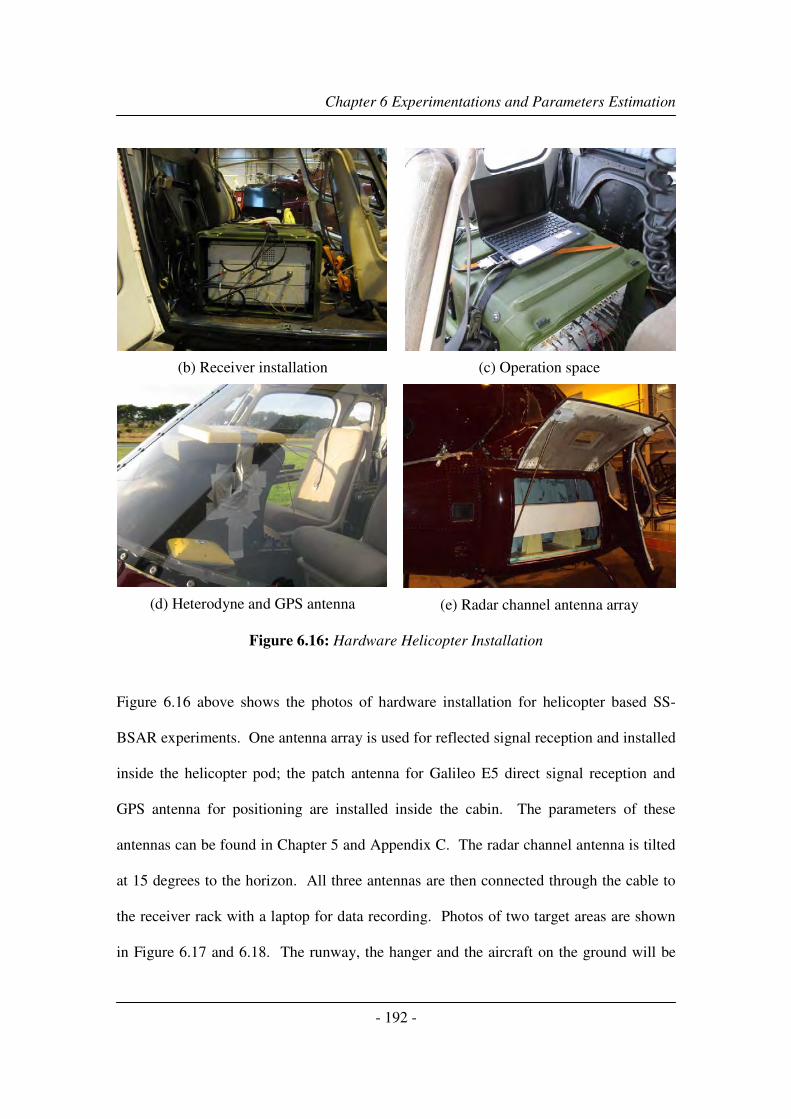
Chapter 6 Experimentations and Parameters Estimation
- 192 -
(b) Receiver installation
(c) Operation space
(d) Heterodyne and GPS antenna
(e) Radar channel antenna array
Figure 6.16: Hardware Helicopter Installation
Figure 6.16 above shows the photos of hardware installation for helicopter based SS-
BSAR experiments. One antenna array is used for reflected signal reception and installed
inside the helicopter pod; the patch antenna for Galileo E5 direct signal reception and
GPS antenna for positioning are installed inside the cabin. The parameters of these
antennas can be found in Chapter 5 and Appendix C. The radar channel antenna is tilted
at 15 degrees to the horizon. All three antennas are then connected through the cable to
the receiver rack with a laptop for data recording. Photos of two target areas are shown
in Figure 6.17 and 6.18. The runway, the hanger and the aircraft on the ground will be

Chapter 6 Experimentations and Parameters Estimation
- 193 -
used for detection. Experimental imaging results will be given and discussed in section
7.4.
Figure 6.17: Target Area 1 – East Fortune Airfield
Figure 6.18: Target Area 2 – PDG Airfield

Chapter 6 Experimentations and Parameters Estimation
- 194 -
6.5 Parameters Estimation
The formation of the synthetic aperture requires a coherent phase history to be
maintained during the time it takes to synthesize the aperture. In fact, three specific
factors impact the phase coherence of the two-dimensional SAR signal and introduce
phase effects that influence the processing complexity and the resulting image quality.
These factors are: propagation, source coherence (synchronisation between transmitted
and reference signals) and motion compensation [2].
SAR imaging from space may encounter significant ionospheric dispersive effects
resulting in phase errors in the range dimension which are caused by the frequency-
dependant index of refraction. A variation in the integrated refractive index between the
radar antenna and the targets also cause azimuth phase errors. Nevertheless the study of
propagation effects on phase coherence of SAR signals is out of scope of this thesis.
There are many excellent articles and books available for this topic [3-6].
For source coherence/synchronisation considerations, it is normal to generate a separate
reference signal, at the appropriate time, using the coherent reference oscillator to
maintain phase coherence in a monostatic SAR system. There are also simpler methods
available for synchronisation between the transmitter and the receiver in the cooperative
bistatic SAR systems. However, for SS-BSAR using GNSS as a non-cooperative
transmitter, synchronisation is important and a specific chapter (Chapter 4) contributes to
this issue in the thesis.

Chapter 6 Experimentations and Parameters Estimation
- 195 -
To generate a coherent synthetic aperture for fine azimuth resolution in a general SAR
system, synchronisation accounts for relative motion between the transmitter/receiver and
target over time. It can be derived from a deterministic path, measured motion using
integrated sensors or signal derived estimation which uses autofocus techniques in
processor or multiple prominent point processing (PPP) techniques. For the experiments
described in the above sections, the relative motion estimation will be mainly derived
from the deterministic path and measurements from integrated sensors. A description of
signal based motion compensation can be found in [2]. Also there are many classical
papers that discuss motion compensation with well-known algorithms for monostatic
SAR [7-9]. However, for motion compensation in bistatic SAR there are fewer
references available [10-12].

Chapter 6 Experimentations and Parameters Estimation
- 196 -
Figure 6.19: Transmitter and Receiver Trajectories with Motion Errors
In this section we will discuss the necessary motion parameters (position, trajectory and
Doppler information) estimation and compensation to achieve the focused SS-BSAR
image. Figure 6.19 above gives a typical example of SS-BSAR topology with the
platform motion estimation errors. The actual trajectories of both transmitter and
receiver are deviated from their nominal paths. Hence the Doppler shift and phase
estimation will also contain intrinsic errors, which eventually affect the focusing of
BSAR data.

Chapter 6 Experimentations and Parameters Estimation
- 197 -
Different methods are proposed for transmitter/receiver parameters extraction and the
practical one is justified. Two problems, residual Doppler shift and low frequency
motion compensation are briefly discussed. Techniques to compensate non-linear
platform motion errors will be introduced and proved with the experimental results at the
end of this section.
6.5.1 Platform Position/Location Estimation
� Transmitter Trajectory Estimation
A GNSS satellite, when used as the non-cooperative transmitter for SS-BSAR, has a
trajectory that is normally a deterministic path and its geographic coordinates at the
specific time can be extracted, calculated or estimated from different sources of
information.
In general, GNSS satellites broadcast two types of navigation data, Almanac and
Ephemeris. Almanac data contains coarse orbital parameters for all satellites in the
constellation; Ephemeris data, by comparison, contains very precise orbital and clock
corrections for each satellite. For our previous experiments using GLONASS [13] the
real time ephemeris, received by a dual channel GPS/GLONASS receiver, were used to
calculate GLONASS satellite’s coordinates in ECEF (Earth-Center Earth-Fixed). The
Cartesian reference frame and sufficient position accuracy has been used to obtain
imaging results. However, the accuracy of the satellite trajectory derived from the

Chapter 6 Experimentations and Parameters Estimation
- 198 -
ephemeris, sometimes, is not enough for high resolution radar applications, for example,
interferometric SAR.
To obtain the highest-precision civilian GNSS data and products, there is one
international community, the international GNSS service (IGS) which can provide <5 cm
accuracy for GPS satellite orbital position and about 15 cm accuracy for GLONASS
satellite orbital position with known latency [14]. To compare, GNSS satellite broadcast
data generally provides real time orbital accuracy of 100 cm and clocks accuracy of 5 ns
RMS; final international GNSS service data provides orbital accuracy up to 2.5 cm and
clock information within 75 ps RMS. However, the highest precise data can not be
obtained in real time, instead 12-18 days latency is expected.
For the experiments described in sections 6.2-6.4, Galileo satellites have been used as the
transmitter. The international GNSS service does not provide the service for the Galileo
constellation yet; the ephemeris broadcasted from GIOVE A/B (first two Galileo testing
satellites) is lacking in consistency at this stage. Another method is proposed and applied
to meet the requirements, which is based on the prediction of GNSS satellite orbits.
Nevertheless, for the operation of future SS-BSAR using GNSS, the real-time ephemeris
is preferred in terms of the convenience and the international GNSS service data is most
favoured for accuracy reasons. A brief description and explanation is given below for the
method based on the orbital predication.

Chapter 6 Experimentations and Parameters Estimation
- 199 -
There are many different ways to mathematically describe the space orbit, but a number
of schemes each consisting of a set of six parameters are commonly used in astronomy
and orbital mechanics [15]. This is because the problem contains six degrees of freedom.
These correspond to the three spatial dimensions which define position (the x, y, z in
a Cartesian coordinate system) plus the velocity in each of these dimensions. These can
be described as orbital state vectors, but this is often an inconvenient way to represent an
orbit, which is why Keplerian elements are commonly used instead. A Keplerian orbit is
merely an idealized, mathematical approximation at a particular time. Keplerian element
parameters can be encoded as text in a number of formats. The most common of them is
the NASA/NORAD two-line elements (TLE) format [15].
In our case, a computer program [16] is used with the two-line elements to compute the
precise position of a satellite at a particular time. The reference frame of the resulting
coordinates is the Earth-centred inertial (ECI) coordinates produced by the orbital model.
The ECI coordinates are then converted to Earth-centred Earth-fixed Cartesian reference
frame and finally transferred to local coordinates. The coordinate localization is realized
through a 7-parameter transformation; more information regarding this issue is given in
Appendix B. As the resulting satellite coordinates often have a 15 minute interval, an
interpolation process will be necessary during the SAR imaging formation. Two
references [17 and 18] should be considered for interpolation methods of GNSS satellite
orbits. Considering the overall integration time of 30-60 seconds (for our experiments),
the linear interpolation method is applied, which gives satisfactory outputs as verified by
the testing results shown in section 6.5.4.

Chapter 6 Experimentations and Parameters Estimation
- 200 -
Unfortunately, the orbital data in the form two-line elements set does not provide any
kind of accuracy information. According to [19], for a spacecraft in a typical Low Earth
orbit, the accuracy that can be obtained is on the order of 1 km within a few days of the
epoch of the element set. For GIOVE A/B satellites trajectories, real-world benchmarking
results are acquired and analyzed in section 6.5.4. It is revealed that the coordinates
derived from two-line elements data set can provide sufficient accuracy for the estimation
of satellite motion and be used for SS-BSAR imaging formation.
� Receiver Trajectory Estimation
For high resolution SAR imaging, the radar position/velocity history is normally required
with sub-meter precision. In our case, a dual frequency GPS receiver is integrated with
the radar receiver hardware (Chapter 5). However, without differential GPS corrections,
its real-time outputs can only provide meter-level receiver position data.
For our experimental data to achieve better estimation on receiver platform motion, a
Precise Point Positioning method is proposed to improve the real time GPS outputs to
centimetre accuracy. Precise Point Positioning is a post-processed GPS position
estimation technique which generates a high precision autonomous solution. It is derived
from a stored GPS receiver observation file combining with international GNSS service
precise satellite orbit estimation, using non-differenced dual-frequency pseudorange and
carrier phase [20]. The resulting position estimates are often referred to the WGS84

Chapter 6 Experimentations and Parameters Estimation
- 201 -
reference frame. However, these new WGS84 realizations are coincident with the
International Terrestrial Reference Frame (ITRF) at about the 10 centimetre level. This
means that one can consider that ITRF coordinates are also expressed in WGS84 at 10
cm level. The same coordinate localization is applied to the receiver coordinates. Hence
both the transmitter and receiver trajectories can be presented in the one pre-defined local
coordinate reference frame. It is also important to note that the quality of the GPS orbit
and clock estimates, and consequently of the Precise Point Positioning derived positions,
has improved from 10 cm and several nanoseconds in 1994 to about 2 cm and 0.1
nanoseconds in 2003.
Figure 6.20 below gives the block diagram of coordinate extraction process, which is
actually applied to the experiment data. In summary, the Galileo satellite positions at the
specific epoch are obtained by the prediction of its orbit using two-line elements data; the
high-precision receiver positions are obtained by the Precise Point Positioning method
using the stored GPS receiver observation file combining with the IGS precise GPS
satellite orbit data. As a result, with high precision estimations of satellite and receiver
trajectories, their velocity histories, Doppler shift and phase variation can be calculated
for the transmitter-target-receiver geometry. For example, the Doppler shift between the
satellite and the receiver (heterodyne channel) can be written as
1 1 1 1 1 1
2 2 2 2 2 2
0
1
( ) ( ) ( ) ( ) ( ) ( )
( )
n n n n n n n n n n n n
n
S R S R S R S R S R S R
d
n n
X X Y Y Z Z X X Y Y Z Zf f
t t C
− − − − − −
−
− + − + − − − + − + −= ⋅
− ⋅
(6.9)
Satellite coordinates at position n: (Xsn,Ysn,Zsn);

Chapter 6 Experimentations and Parameters Estimation
- 202 -
Receiver coordinates at position n: (Xrn,Yrn,Zrn);
fd: Doppler shift.
fo: Carrier frequency.
C: Speed of light
Figure 6.20: Coordinates Extraction for Transmitter and Receiver
One more thing is worth mentioning regarding receiver position. Although the resulting
receiver coordinates have an accuracy of 2.5 cm, due to Precise Point Positioning
processing, its update rate is 1 Hz from most GPS receivers. This means that the moving
receiver position will be updated every one second; this is usually not adequate for the

Chapter 6 Experimentations and Parameters Estimation
- 203 -
estimation of high frequency motion errors. For example, the airborne platform is
moving with high speed and rapid vibration, the phase centre of the antenna on the
platform will suffer from high frequency motion errors. In such situations, the inertial
measurement unit (IMU) and inertial navigation system (INS) are often required to
provide short-term, high-frequency motion estimation. For the helicopter trials
mentioned in section 6.4, the IMU/INS has not been used because of technical reasons.
Its effect on the SS-BSAR image formation is uncertain and worthy of further study in
the future.
6.5.2 The Problem of Residual Doppler Shift in SS-BSAR
Another problem associated with airborne SS-BSAR is the residual Doppler shift present
between the heterodyne channel and the radar channel. This is due to the fact that the
transmitter and receiver are both in motion, and in addition they are not co-located. This
topology creates a difference in the angular velocity between the satellite-to-target path
(radar channel) and the satellite-to-receiver path (heterodyne channel).
RR, frt(u)
RT, fst(u)
RS, fs(u)
Heterodyne channel
Radar channel
Target Receiver
β
Satellite
Figure 6.21: Bistatic Triangle

Chapter 6 Experimentations and Parameters Estimation
- 204 -
RS: Satellite-to-Receiver range
RT: Satellite-to-Target range
RR: Receiver-to-Target range
fs(u): Doppler variation between satellite and receiver
fst(u): Doppler variation between satellite and target
frt(u): Doppler variation between receiver and target (azimuth signature)
Figure 6.21 above shows the bistatic triangle for BSAR with the range and Doppler shift
parameters. In the monostatic SAR, frt(u) is the source of the azimuth signal and forming
the azimuth resolution. However, this is not the case for BSAR because fs(u) is often not
equal to fst(u). This residual Doppler shift (fst(u)- fs(u)) can be large enough to introduce a
complete mismatch in the Doppler histories between the heterodyne channel and the
radar channel. It could be space-variant and time-variant. It should be noted that this
problem of a moving heterodyne channel is not only restricted to SS-BSAR using GNSS
transmitters, but also a key problem of airborne SS-BSAR using any transmitter. In this
section we will comprehensively discuss the problem of residual Doppler shift and how it
affects the imaging algorithm. A method to estimate the residual Doppler shift will be
described.
To describe the assumption made by the imaging algorithm, the received signal at the
heterodyne channel can be expressed as:

Chapter 6 Experimentations and Parameters Estimation
- 205 -
( )h s
( )s (t,u) p t- exp -j2 ( ) t
C
SR u
f uπ
= ×
(6.10)
where t denotes fast time and u denotes slow (azimuth) time, p is the envelope of the
ranging signal, c is the speed of light, ( )SR u is the satellite-to-heterodyne range, varying
with azimuth time u and s ( )f u is the Doppler shift experienced by received heterodyne
signal.
The signal received at the radar channel is given by:
( )r st
( ) ( )s (t,u) p t exp -j2 ( ) ( ) t
C C
T Rrt
R u R uf u f uπ
= − − × +
(6.11)
where ( )TR u and ( )RR u are satellite-to-target and receiver-to-target range respectively,
st ( )f u is the Doppler shift due to the satellite motion relative to the target at
coordinates ( )tata yx , and )(ufrt is the Doppler shift due to the receiver motion relative to
the target. This Doppler shift )(ufrt forms the main azimuth signature for image
formation.
For each aperture position, the range/delay ( )
SR u
C and Doppler shift
s ( )f u were found
from the synchronisation algorithm (discussed in Chapter 4). During the range
compression, range and Doppler shifts were then removed from the radar channel signal
which was stored for that particular position. Hence, the signal returned from a single

Chapter 6 Experimentations and Parameters Estimation
- 206 -
point target at coordinates ( )tata yx , after the range ( )SR u and the corresponding Doppler
shift s ( )f u are removed, has the form:
( )
( )
rh
( )( ) ( )s (t,u) p t exp -j2 ( ) ( ) ( ) t
( )( ) p t exp -j2 ( ) ( ) t
SR Tst rt s
reRre rt
R uR u R uf u f u f u
c c c
R uR uf u f u
c c
π
π
= − + − × + −
= − + × ∆ +
(6.12)
( ) ( ) ( ) and ( ) ( ) ( )re T S re s stR u R u R u f u f u f u= − ∆ = − (6.13)
It could be seen from the above equations that the terms ( )reR u and ( )ref u∆ introduce a
residual range migration and a residual Doppler shift. A method to estimate the residual
Doppler shift in the heterodyne channel was experimentally verified using the
GLONASS satellite [21]. The experimental results are given in section 6.5.4 using a
Galileo satellite. In the above equations, the azimuth signature )(ufrt is formed by the
motion of the radar channel antenna relative to the target. Therefore in the imaging
algorithm, an appropriate azimuth filter is designed for each range bin accordingly. A
detailed explanation of the imaging algorithm is outside the scope of this thesis and can
be found in [22, 23].
6.5.3 Motion compensation
Motion compensation (MC) is another aspect of SAR phase coherence. For BSAR,
motion compensation is required for two platforms, instead of one platform in the

Chapter 6 Experimentations and Parameters Estimation
- 207 -
monostatic SAR case. However, the objectives and the effects remain more or less same.
High frequency motion errors cause a loss in dynamic range, i.e., degraded sidelobe and
resolution loss. Low frequency motion errors cause geometric distortion and poor map
accuracy [7]. Motion compensation will not be perfect, with a residual phase error
remaining in the signal. In general, the minimum objective is to reduce motion-induced
phase effects to a level that an autofocus algorithm can accommodate.
There are three types of relative motion, line-of-sight translational, rotational motion and
motion of individual targets. The tolerable magnitude of uncompensated motion
increases with radar centre frequency, because the phase error associated with an
uncompensated distance varies inversely with wavelength. At a given wavelength, the
tolerable uncompensated distance is relatively independent of azimuth resolution, but
resolution does naturally impact the allowable velocity or acceleration measurement
error, since the resulting motion error increases with aperture time. It is common practice
to use π/4 radian as an acceptable level of uncompensated low-frequency, nonlinear
phase errors in order to avoid significant deterioration in image quality. First order
bistatic motion compensation can be expressed as
( )2 2
'( ) ( ) ( )err
R t R t R tπ π
ϕλ λ
= − = ∆ (6.14)
'( ) '( ) ( ) ( ) ( ) ( )'( ) ( )R T R T R T
D
V t V t V t V t V t V tf t
λ λ λ λ λ λ
∆ ∆= + = + + + (6.15)

Chapter 6 Experimentations and Parameters Estimation
- 208 -
The correction term is ( ) ( )
( ) R TD
V t V tf t
λ λ
∆ ∆∆ = + to compensate for the shift of the
azimuth spectrum.
Moreover, antenna phase centre position/motions create phase effects in the SAR signal
history. The antenna is normally suffering short-tem fluctuations in three dimensions.
Measurement of the antenna phase centre motion requires a position history with
accuracy over both the short and the long terms. In practice, GPS provides high long
term accuracy with poor data rate and noisy attitude. INS provides high short term
accuracy with high data rate and accurate attitude resolution. So GPS/INS integration,
using a Kalman filter is a sufficient solution for motion compensation in SS-BSAR
application.
6.5.4 Parameter Estimation Results
In this section, parameter estimation results are discussed and analyzed based on one
ground moving receiver experiment (short aperture), which is described in section 6.3.
The results are provided for transmitter/receiver coordinates, velocities, Doppler shifts
and phase histories. For satellite parameters, the outcomes are compared between
predications using a two-line elements data set and broadcast satellite position. Motion
compensation results are shown for the relative non-linear motion between the transmitter
and the receiver platforms. It is clearly shown from these results that the proposed
methods and techniques are sufficient and effective for parameter estimation from our
experiment data.

Chapter 6 Experimentations and Parameters Estimation
- 209 -
0 5 10 15 20 25 30 352.3513
2.3514
2.3514
2.3514
2.3515
2.3516
2.3516
2.3516
2.3517x 10
7
Time, s
Ran
ge,
m
global
local
(a) baseline range
0 5 10 15 20 25 30 35-4
-2
0
2
4
6
8x 10
-9
Time, s
Ran
ge d
iffe
rence
, m
localization errors
(b) localization errors
Figure 6.22: Coordinate Localization
Figure 6.22 verifies the outputs of coordinate localization (refer to Appendix B). Figure
6.22(a) plots the range history between the transmitter and the receiver using the
coordinates, both in the global reference frame and in the local frame. The range
histories are almost identical and it can be seen from Figure 6.22(b) that the error in range
history is on the order of 10-9
m because of the localization process. Then all estimation
can be based on the local coordinates for Doppler shift, phase history etc.
-1-0.5
00.5
-200-1000100200
-1.5
-1
-0.5
0
0.5
1
1.5
2
2.5
X, mY, m
Z,
m
real time
LMS
(a) receiver trajectory
0 5 10 15 20 25 307
7.2
7.4
7.6
7.8
8
8.2
8.4
8.6
8.8
9
Time, s
Velo
city,
m/s
real time
LMS
(b) receiver velocity

Chapter 6 Experimentations and Parameters Estimation
- 210 -
0 5 10 15 20 25 30 350
0.2
0.4
0.6
0.8
1
1.2
1.4
Time, s
Err
or,
m
(c) baseline range error due to receiver
estimation error
0 5 10 15 20 25 30-1
-0.8
-0.6
-0.4
-0.2
0
0.2
0.4
0.6
0.8
1
Time, s
Err
or,
m/s
(d) receiver velocity error
Figure 6.23: Receiver Parameters Estimation
Figure 6.23 shows the result of the receiver parameters estimation from the Precise Point
Positioning method proposed previously. It includes the receiver trajectory and velocity
in the local reference frame. Figures 6.23(a) and 6.23(b) also give the least mean square
outputs of estimated receiver path and velocity with a red line. It can be seen that least
mean square receiver path has been defined as the Y-axis for the local frame in this case.
Figure 6.23(c) presents the errors of bistatic baseline range estimation, due to receiver
non-linear motion. Its maximum deviation is around 1.4 m from its nominal path and
velocity error is around 0.4 m/s at the maximum (considering nominal speed ~ 8 m/s).
Figure 6.23(d) shows the result of receiver velocity estimation errors and clearly reveals
the acceleration and deceleration phase of receiver motion.
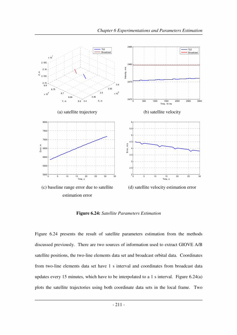
Chapter 6 Experimentations and Parameters Estimation
- 211 -
3.4
3.45
3.5
3.55
3.6
x 106
8.6
8.65
8.7
8.75
8.8
x 106
2.15
2.155
2.16
2.165
x 107
X, mY, m
Z,
m
TLE
Broadcast
(a) satellite trajectory
0 500 1000 1500 2000 2500 30002470
2475
2480
2485
Time, 10 ms
Velo
city,
m/s
TLE
Broadcast
(b) satellite velocity
0 5 10 15 20 25 30 355000
5500
6000
6500
7000
7500
8000
Time, s
Err
or,
m
(c) baseline range error due to satellite
estimation error
0 5 10 15 20 25 302
2.5
3
3.5
4
4.5
5
5.5
6
Time, s
Err
or,
m/s
(d) satellite velocity estimation error
Figure 6.24: Satellite Parameters Estimation
Figure 6.24 presents the result of satellite parameters estimation from the methods
discussed previously. There are two sources of information used to extract GIOVE A/B
satellite positions, the two-line elements data set and broadcast orbital data. Coordinates
from two-line elements data set have 1 s interval and coordinates from broadcast data
updates every 15 minutes, which have to be interpolated to a 1 s interval. Figure 6.24(a)
plots the satellite trajectories using both coordinate data sets in the local frame. Two

Chapter 6 Experimentations and Parameters Estimation
- 212 -
results are separated far away and a constant shift is observed. Figure 6.24(b) plots the
velocities derived from two different satellite paths. Velocity from broadcast data is
almost constant over the 30 s integration time; velocity from the two-line elements data is
varying slowly, in this case, increasing. Figure 6.24(c) presents the errors of bistatic
baseline range estimation due to different satellite position estimations. This error is not
constant and it varies from around 6000 m to 7000 m during the synthetic aperture.
However, comparing to the Galileo satellite orbit height of 23000 km, the effect of this
error may be neglected. Figure 6.24(d) shows the result of satellite velocity estimation
errors and it is between 3.5 m/s to 4.5 m/s comparing to the average satellite speed of
2500 m/s. It will be shown from the results below that surprisingly, the two-line
elements data provides a closer match to the parameters tracked by the synchronisation
algorithm than the broadcast satellite position.
0 5 10 15 20 25 30 352.3519
2.352
2.352
2.3521
2.3521
2.3522
2.3522
2.3523
2.3523
2.3523
2.3524x 10
7
Time, s
Ran
ge,
m
real time
LMS
(a) baseline range history estimation
1.02 1.04 1.06 1.08 1.1 1.12 1.14 1.16 1.18
2.3519
2.3519
2.3519
2.3519
2.3519
2.3519x 10
7
Time, s
Ran
ge,
m
real time
LMS
(b) zoom

Chapter 6 Experimentations and Parameters Estimation
- 213 -
0 5 10 15 20 25 30154
154.2
154.4
154.6
154.8
155
155.2
155.4
155.6
Time, s
Ran
ge r
ate
, m
/s
real time
LMS
(c) range rate estimation
0 5 10 15 20 25 30620
621
622
623
624
625
626
627
Time, s
Fre
qu
en
cy,
Hz
real time
LMS
(d) Doppler shift estimation
Figure 6.25: Baseline Range and Doppler History Estimation
After the trajectories and velocities of the transmitter and receiver are estimated, Doppler
shift could be calculated. Figure 6.25 shows the result of bistatic baseline range history,
range rate and Doppler shift history estimation. The satellite positions derived from the
two-line elements set is used; both real-time receiver positions and least mean square
output of the receiver positions are used for comparison. Figure 6.25(a) shows the
bistatic baseline range history using real-time and least mean square output of the
receiver paths. This is slightly different from the plot shown in Figure 6.22(a), which is
derived from same coordinates but in a different reference frame. From Figure 6.25(b), it
can be seen that there is a small mismatch. The range rate can then be easily calculated
from the range history between the transmitter and receiver, (Figure 6.25(c)) and
converted to the Doppler shift in the heterodyne channel. The same Doppler shift is also
tracked by the synchronisation algorithm. There is about 5 Hz Doppler bandwidth for 30
s aperture time. From Figures 6.25(c) and 6.25(d), we can see that the range rate or
Doppler shift derived from least mean square output of receiver positions is linearly
changing (red line), but the real-time value is varying mainly due to the actual non-linear
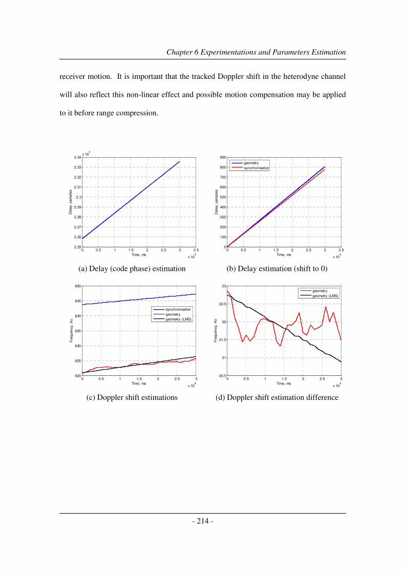
Chapter 6 Experimentations and Parameters Estimation
- 214 -
receiver motion. It is important that the tracked Doppler shift in the heterodyne channel
will also reflect this non-linear effect and possible motion compensation may be applied
to it before range compression.
0 0.5 1 1.5 2 2.5 3 3.5
x 104
2.25
2.26
2.27
2.28
2.29
2.3
2.31
2.32
2.33
2.34x 10
4
Time, ms
Dela
y,
sa
mp
les
(a) Delay (code phase) estimation
0 0.5 1 1.5 2 2.5 3 3.5
x 104
0
100
200
300
400
500
600
700
800
900
Time, ms
Dela
y,
sa
mp
les
geometry
synchronisation
(b) Delay estimation (shift to 0)
0 0.5 1 1.5 2 2.5 3
x 104
620
625
630
635
640
645
650
Time, ms
Fre
qu
en
cy,
Hz
synchronisation
geometry
geometry (LMS)
(c) Doppler shift estimations
0 0.5 1 1.5 2 2.5 3
x 104
20.5
21
21.5
22
22.5
23
Time, ms
Fre
qu
en
cy,
Hz
geometry
geometry (LMS)
(d) Doppler shift estimation difference

Chapter 6 Experimentations and Parameters Estimation
- 215 -
0 20 40 60 80 1000
1
2
3
4
5
6
7
Time, ms
Pha
se,
radia
n
synchronisation
geometry
(e) phase history estimation
100 120 140 160 180 2000
1
2
3
4
5
6
7
Time, ms
Pha
se,
radia
n
real time
LMS
(f) phase spectrum
Figure 6.26: Comparison between Synchronisation Results and Parameters Estimation
Results
Figure 6.26 above provides the comparison between synchronisation results (Chapter 4)
and parameters estimation results in the heterodyne channel. One is derived from the
heterodyne channel signal and the other is derived from a geometrical approach.
Figure 6.26(a) plots the delay variation, which is derived from the baseline range history
(Figure 6.25(a)). Figure 6.26(b) presents the comparison between this delay and the
tracked delay (red line). The tracked value is from the delay-tracking loop of the
proposed synchronisation algorithm. Both results are shifted to a start value of 0.
Because the tracked value is a relative delay (code phase) measurement, it follows and
extracts the change of delay without the information about the initial delay due to the
transmitter-to-receiver range. One thing to mention here is that this initial delay could be
found from the difference between the time of the signal being transmitted (included in
the ephemeris) and the time of signal arrival. It can be seen that there is a divergence

Chapter 6 Experimentations and Parameters Estimation
- 216 -
between the two estimated delays, which is increasing with the time. This is mainly
because the tracked delay not only presents the geometry motion between transmitter and
receiver, but also includes the errors due to the propagation, local oscillator shifts, clock
slippage etc.
Figure 6.26(c) shows the tracked Doppler shift and those from the geometry approach.
The tracked Doppler shift are the values after least mean square fitting is applied to the
actual Doppler shift tracking outputs. It is changing linearly without any non-linear
component. However, the actual tracked Doppler shift is varying within about a 15 Hz
range due to receiver noise (Figure 4.17). The other two plots in the figure are the same
as Figure 6.25(d), which is the Doppler shift, estimated from the geometry coordinates.
We can see a similar Doppler shift changing rate achieved by the two sources, but also
there is a varying shift between the two sets of results, shown in Figure 6.26(d). The shift
is ~ 22 Hz for this set of data, mainly coming from the clock offset between the
transmitter and the receiver. Its value corresponds to the frequency accuracy ±25 Hz of
the radar hardware (described in Chapter 5). So the difference between the two Doppler
shift estimation techniques is mainly because of the frequency deviation of the local
oscillator (frequency synthesizer) in the radar hardware. Figure 6.27 below will provide
further proof for this assumption and the possible compensation that can be applied.
Figure 6.26(e) plots the phase variations (100 ms data) extracted by the tracking
algorithm (blue line) and that derived from the range history (red line). Obviously the
two estimated phases would not match each other as the two estimated Doppler shifts

Chapter 6 Experimentations and Parameters Estimation
- 217 -
have a varying shift. However, compensation schemes can be designed and tested using
the frequency spectrum derived from these phases. Figure 6.26(f) presents the phase
results derived from the range history, using real-time and least mean square output of
receiver positions. It can be seen that the phases are almost overlapped with minor
differences.
615 620 625 630 635 640 645 650 6550
0.1
0.2
0.3
0.4
0.5
0.6
0.7
0.8
0.9
1
Frequncy, Hz
Mag
nitu
de
synchronisation
geometry
geometry (LMS)
(a) phase spectrum
615 620 625 630 635 640 645 650 6550
0.1
0.2
0.3
0.4
0.5
0.6
0.7
0.8
0.9
1
Frequncy, Hz
Mag
nitu
de
synchronisation
geometry
geometry (compensated)
(b) phase spectrum
640 642 644 646 648 6500
0.1
0.2
0.3
0.4
0.5
0.6
0.7
0.8
0.9
1
Frequncy, Hz
Mag
nitu
de
synchronisatio
compensated
(c) phase spectrum (constant frequency shift compensation)

Chapter 6 Experimentations and Parameters Estimation
- 218 -
640 642 644 646 648 6500
0.1
0.2
0.3
0.4
0.5
0.6
0.7
0.8
0.9
1
Frequncy, Hz
Mag
nitu
de
synchronisation
compensated
(d) compensated phase spectrum (zoom of (b))
Figure 6.27: Motion Compensation (vehicle trial data)
Figure 6.27 shows the frequency spectrum derived from the estimated phase variation
and results of motion/phase compensation. Three phase spectrum are plotted in Figure
6.27(a), they are derived from the tracked phase (blue line) and the phase calculated from
the transmitter/receiver range histories (red line from the motion between the satellite
positions and real-time receiver positions; black line using least mean square output of
receiver positions). These phases are actually corresponding to the Doppler shift in
Figure 6.26(c), with the only difference in the tracked results. The tracked phase
spectrum (blue line) presents the actual frequency/phase variation, but the Doppler shift
in Figure 6.26(c) is the least mean square output. It can be seen that the tracked phase
spectrum and the real-time geometry derived phase spectrum have similar patterns and
fluctuations, for example, three high magnitude spikes. From these results, the tracking

Chapter 6 Experimentations and Parameters Estimation
- 219 -
(synchronisation) algorithm have been verified again; it clearly tracked and extracted the
non-linear receiver motion.
Subsequently appropriate motion/phase compensation can be applied to both the directly
received signal (heterodyne channel) and the reflected signal, for any undesired motion
effects. Here we will only show the initial results of motion compensation applied to the
heterodyne signal in SS-BSAR. Figure 6.27(b) again plots three phase spectrum, where
the compensated phase spectrum is displayed as a black line. The proposed
compensation is by shifting the red spectrum (geometry derived value) with the
difference between the least mean square output of tracked Doppler shift and the
geometry results, which is shown in Figure 6.26(d). It can be seen that a linear frequency
modulated (LFM) signal (Figure 6.27(d)) is achieved after the phase compensation, hence
the non-linear receive motion effect has been removed. Figure 6.27(c) shows the tracked
phase spectrum and the geometry results compensated by a fixed value (21.5 Hz in this
case). It can be seen that the two phase spectrum are not exactly the same, with small
discrepancies due to the propagation or clock slippage, which is tracked by the
synchronisation algorithm.

Chapter 6 Experimentations and Parameters Estimation
- 220 -
610 620 630 640 650 660 670 680 690 7000
0.1
0.2
0.3
0.4
0.5
0.6
0.7
0.8
0.9
1
Frequncy, Hz
Mag
nitu
de
synchronisation
geometry
geometry (LMS)
(a) phase spectrum (motion error
compensation)
610 620 630 640 650 660 670 680 690 7000
0.1
0.2
0.3
0.4
0.5
0.6
0.7
0.8
0.9
1
Frequncy, Hz
Mag
nitu
de
synchronisation
geometry
compensated
(a) phase spectrum (motion error
compensation)
660 665 670 675 680 685 690 6950
0.1
0.2
0.3
0.4
0.5
0.6
0.7
0.8
0.9
Frequncy, Hz
Mag
nitu
de
synchronisation
compensated
(c) compensated phase spectrum by fix frequency shift

Chapter 6 Experimentations and Parameters Estimation
- 221 -
660 665 670 675 680 685 690 6950
0.1
0.2
0.3
0.4
0.5
0.6
0.7
0.8
0.9
1
Frequncy, Hz
Mag
nitu
de
synchronisation
compensated
(d) compensated phase spectrum (zoom of (b))
Figure 6.28: Motion Compensation (helicopter trial data)
Figure 6.28 gives another example of motion/phase compensation. They are based on the
helicopter trial data which is described in section 6.4. Similarly, three phase spectrum are
plotted in Figure 6.28(a), they are derived from the tracked phase (blue line) and the
phase calculated from the transmitter/receiver range histories (red line from the motion
between the satellite positions and real-time receiver positions; black line using least
mean square output of receiver positions). The tracked phase spectrum (blue line)
presents the actual frequency/phase variation. It can be seen that the tracked phase
spectrum and the real-time geometry derived phase spectrum have similar patterns and
fluctuations, for example, multiple high magnitude spikes and a relative flat band around
the centre. From these results, we can say that the tracking algorithm clearly tracked and

Chapter 6 Experimentations and Parameters Estimation
- 222 -
extracted the non-linear motion of the helicopter platform. Figure 6.28(b) again plots the
compensated phase spectrum in a black line. It can be seen that a linear frequency
modulated (LFM) signal (Figure 6.28(d)) is achieved after the phase compensation, hence
the non-linear receive motion effect has been removed. Figure 6.28(c) shows the tracked
phase spectrum and the geometry results compensated by a fixed value (56.3647 Hz in
this case). It can be seen that the two phase spectrum are not exactly same, with a small
discrepancy due to the propagation or clock slippage, which is tracked by the
synchronisation algorithm.
6.6 Summary
This chapter consists of two main parts. The first part introduces the programme of
experimentation leading to airborne SS-BSAR imaging. Experimental strategies and
trials plans are designed to confirm the system performance. It has been divided into
three stages: stationary receiver, ground moving receiver and airborne receiver. The
actual experimental parameters and set-up block diagrams are also given.
The second part discusses the parameter estimation requirement for the proposed SS-
BSAR system. Before applying the image formation algorithm to the experimental data,
the parameters, such as, the transmitter/receiver trajectories, Doppler shift and phase
histories need to be estimated with known accuracy. Two problems, residual Doppler
shift and motion compensation are briefly discussed. The practical methods are proposed
for transmitter/receiver parameter extraction and compensation. The estimation results
from the real experimental data are discussed at the end of the chapter.

Chapter 6 Experimentations and Parameters Estimation
- 223 -
References
1. Ruck, G.T., et al., Radar Cross Section Handbook. Vol. 2. 1970: Plenum press.
2. Carrara, W., R. Goodman, and R. Majewski, Spotlight Synthetic Aperture Radar:
Signal Processing Algorithms. 1995: Artech House.
3. Banks, P.M. and G. Kockarts, Aeronomy. Vol. A and B. 1973, San Diego,
Califorinia: Academic.
4. Bauer, S.J. and H. Lammer, Physics of Earth and Space enviroments. 2004,
Berlin: Springer.
5. Kelley, M.C., Ionospheric Plasma Dynamics. 1989, San Diego, California:
Academic.
6. Parks, G.K., Physics of Space Plasma: An Introduction. 2nd ed. 2004, Boulder,
Colorado: Westview Press.
7. Kirk, J.C., Motion Compensation for Synthetic Aperture Radar. IEEE
Transactions on Aerospace and Electronic Systems, 1975. AES-11(3).
8. Mims, J.H. and J.L. Farrell, Synthetic Aperture Imaging with Maneuvers. IEEE
Transactions on Aerospace and Electronic Systems, 1972. AES-8(4).
9. Kennedy, T.A., Strapdown inertial measurement units for motion compensation
for synthetic aperture radars. IEEE Aerospace and Electronic Systems Magazine,
1988. 3(10): p. 32-35.
10. Nies, H., et al., Parameter estimation for bistatic constellations, in Geoscience
and Remote Sensing Symposium, 2005. IGARSS '05. 2005. p. 1038-1042.
11. Nies, H., et al., A Solution for Bistatic Motion Compensation, in Geoscience and
Remote Sensing Symposium, 2006. IGARSS 2006. IEEE International Conference.
2006. p. 1204-1207.
12. Zhenbo, Z., T. Ziyue, and J. Xingzhou, Research on Bistatic SAR Motion
Compensation, in Radar, 2006. CIE '06. International Conference. 2006. p. 1-4.
13. Cherniakov, M., et al., Bistatic Synthetic Aperture Radar with Emitters of
Opportunity. 2006, Unversity of Birmingham: Birmingham.
14. Dow, J.M., R.E. Neilan, and C. Rizos, The International GNSS Service in a
changing landscape of Global Navigation Satellite Systems. Journal of Geodesy,
2009(83): p. 191–198.
15. Celestrak. Available from: http://celestrak.com/.
16. Okan, V., GPS, http://www.movingsatellites.com/.
17. Hofmann-Wellenhof, Lichtenegger, and Collins, GPS: Theory and Practice. 5th
ed. 2001: Springer.

Chapter 6 Experimentations and Parameters Estimation
- 224 -
18. Schenewerk, A brief review of basic GPS orbit interpolation strategies. GPS
Solutions, 2003(6): p. 265-267.
19. Kelso, T.S., Validation of SGP4 and IS-GPS-200D Against GPS Precision
Ephemerides, in 17th AAS/AIAA Space Flight Mechanics Conference. 2007:
Sedona, AZ.
20. GPS Point Positioning Service CSRS - Precise Point Positioning (PPP).
Available from:
http://webapp.csrs.nrcan.gc.ca/index_e/products_e/online_data_e/online_data_e.h
tml.
21. Saini, R., R. Zuo, and M. Cherniakov, Problem of Signal Synchronisation in SS-
BSAR based on Global Navigation Satellite Emissions - Experimental Results.
IET Proceedings Radar, Sonar and Navigation, 2009. 4(1): p. 110 - 125.
22. Antoniou, M., M. Cherniakov, and C. Hu, Space-Surface Bistatic SAR Image
Formation Algorithms. Geoscience and Remote Sensing, IEEE Transactions on
2009. 47(6): p. 1827 - 1843.
23. Antoniou, M., R. Saini, and M. Cherniakov, Results of a Space-Surface Bistatic
SAR Image Formation Algorithm. Geoscience and Remote Sensing, IEEE
Transactions on 2007. 45(11): p. 3359 - 3371

Chapter 7 Experimental Results and Image Analysis
- 225 -
Chapter 7 Experimental Results and Image Analysis
7.1 Image Formation Overview
In this section, a conceptual description of two BSAR image formation algorithms will be
provided, which have been applied to the experimental data. However, before
proceeding with our analysis, it is important to describe the structure of the BSAR
collected data, to explain the need for and the purpose of SAR image formation
algorithms in general, and to provide a brief background of general methods used for
SAR signal compression.
The raw SAR data, collected during aperture synthesis, are assumed to be recorded in
two dimensions. The first one is defined as the fast-time (or range-time) dimension; it is
associated with propagation delays between signal transmission and echo reception. The
second is defined as the slow-time (or azimuth-time) dimension; this is used in the
specification of the radar’s position during array synthesis. The reason for this notation is
that the signals’ propagation speed (the speed of light) is much faster than the speed of
the transmitter/receiver platforms. Conceptually then, data collection proceeds as
follows: In each radar position (corresponding to an instant in slow-time), the radar stops,
transmits a pulse, records the pulse’s echoes from the imaging area over a pre-defined
time interval in the fast-time domain, and then advances to the next position. This is
commonly known as the stop-and-go assumption.

Chapter 7 Experimental Results and Image Analysis
- 226 -
Now, if we consider a single point target within an imaging area, the transmitter-to-
target-to-receiver time, and hence the target’s apparent range from the radar, varies as the
radar moves from one position to another (i.e. it varies with slow-time). If the range
variation is greater than the system’s range resolution, this effect is known as range cell
migration (range cell migration) and needs to be corrected, since the signal’s energy is
now distributed along several range bins. After range cell migration correction, the
signal’s energy is concentrated in one range bin, corresponding to the target’s range of
closest approach to the radar. Correction of range cell migration is an integral part of
SAR signal processing, and the way it is performed often constitutes the main difference
between some SAR algorithms.
Once the SAR data have been collected from the observation area and demodulated by
the coherent microwave receiver, it is the purpose of SAR processing to produce an
image by mapping target echoes from within that area into an evenly spaced ( )yx, output
grid. The x-coordinate represents ‘forward’ range (perpendicular to the synthesized
array) and the y-coordinate represents lateral range, otherwise known as cross-range. The
targets’ forward ranges can be found from the relevant signal propagation delays, to and
from the radar (fast-time information); their lateral ranges can be found from their
azimuth phase signatures (slow-time information).
Whereas some of the monostatic SAR algorithms have previously existed for decades,
interest in BSAR algorithms has risen only in the last few years. BSAR algorithms exist

Chapter 7 Experimental Results and Image Analysis
- 227 -
which process data, partially, in the time domain but, as far as the author is aware, a
generalized, entirely frequency domain, precision BSAR algorithm (such as the RDA,
range cell migration, CSA) is not yet available. Here “generalized” means an algorithm
which is able to process data collected with the transmitter and receiver flying in non-
parallel flight paths, with unequal velocities.
A plan view of a general BSAR data collection geometry is shown in Figure 7.1. The
transmitter and receiver are moving along the paths with velocities RT VV , , respectively,
so that their synthetic aperture lengths during the data collection time are unequal. The
cross-range direction y is defined to be the same as the receiver’s moving path, and the
range direction x is perpendicular to y . For a point target at coordinates ( )00 , yRR , the
instantaneous transmitter-to-target and receiver-to-target slant ranges )(uRT and )(uRR
are given by:
( ) ( )2
0
22
0 uuVRuR TTTT −+= (7.1)
( ) ( )2
0
22
0 uuVRuR RRRR −+= , (7.2)
where 00 , RT RR are the transmitter’s and receiver’s slant ranges of closest approach to the
target, occurring at slow-times 00 , RT uu , with
00 RRuVy = .

Chapter 7 Experimental Results and Image Analysis
- 228 -
Figure 7.1: General BSAR Geometry (2D view)
Assuming the target is within the transmitting and receiving antennas’ mainlobe for the
whole integration time, then after baseband demodulation, the received signal from this
point target is given by:
( )( ) ( ) ( ) ( )
+−
−−=
c
uR
c
uRfj
c
uR
c
uRtputs RT
c
RT π2exp, (7.3)
where the azimuth signal’s envelope has been omitted. From Equation 7.3, we see that
the round trip two-way propagation delay of the monostatic signal has been replaced by

Chapter 7 Experimental Results and Image Analysis
- 229 -
the two-path (transmitter-target and target-receiver) time delay in the bistatic signal; the
different time delay, and delay variation, implies different signal phase, and phase
variation. The slant ranges of closest approach are different for the transmitter and the
receiver. Moreover, since the transmitter and the receiver move in different trajectories
and their aperture lengths are different, )(uRT and )(uRR vary differently with slow-
time. As a result, the total range cell migration is the sum of two individual and different
range cell migrations, one due to the transmitter’s motion, the other due to the receiver’s.
As far as phase variation across the aperture is concerned, we see from Equation 7.3 that
this is the sum of two independent and different modulations, one due to the transmitter’s
motion relative to the target, and one due to the receiver’s.
As in the monostatic case, the most straightforward way to process the signal in (7.3) is
by two-dimensional matched filtering in the time domain. Note that each received fast-
time sample corresponds to the range sumRT RR + , however we want each output grid
point in the image to represent range and cross-range respect to the receiver. Therefore,
for each output grid point ( )RjiR uR ,0 , i.e. for each target at these coordinates, the
transmitter-to-target and receiver-to-target range histories are given by:
( )( ) ( )222
0, uuVRuR TjTiTjiT −+= (7.4)
( )( ) ( )222
0, uuVRuR RjRiRjiR −+= , (7.5)

Chapter 7 Experimental Results and Image Analysis
- 230 -
where iRiT RR 00 , are the transmitter’s and receiver’s slant ranges of closest approach to the
target, occurring at time RjTj uu , . Then the filter’s response for the particular grid point
can be written as:
( ) ( )( ) ( ) ( ) ( ) ( ) ( ) ( )
+−
−−=
c
uR
c
uRfj
c
uR
c
uRtputs
jiRjiT
c
jiRjiT ,,,,
0 2exp, π (7.6)
and the matched filtering operation is given by:
( ) ( ) ( )∑∑ ×=t u
RjiR utsutsuRf ,,,*
00, (7.7)
where the double sum is over all the available values of ( )ut, .
The similarity between (7.7) and the monostatic matched filtering operation is evident.
However, there are some fundamental differences. In the monostatic case, in order to
calculate the filter’s response at a particular grid point, we need only to calculate the
round-trip range of closest approach (of the radar to the target) and the corresponding
azimuth time. Image formation calculations are straightforward, since the sample
spacings of the output grid in the range-time and azimuth-time dimensions coincide with
the sample spacings of the received signal (input to the SAR processor), and they are
uniform. For the bistatic case, in order to calculate the filter’s response at a particular
output grid point, we need to find both the transmitter’s and the receiver’s ranges of
closest approach and their corresponding azimuth times. This means that, for each output
point, most of the parameters need to be recalculated. Furthermore, as mentioned
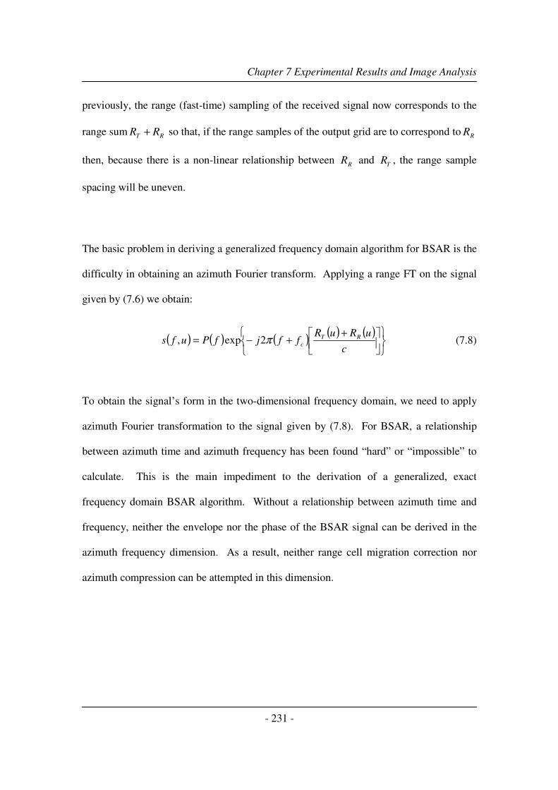
Chapter 7 Experimental Results and Image Analysis
- 231 -
previously, the range (fast-time) sampling of the received signal now corresponds to the
range sum RT RR + so that, if the range samples of the output grid are to correspond to RR
then, because there is a non-linear relationship between RR and
TR , the range sample
spacing will be uneven.
The basic problem in deriving a generalized frequency domain algorithm for BSAR is the
difficulty in obtaining an azimuth Fourier transform. Applying a range FT on the signal
given by (7.6) we obtain:
( ) ( ) ( )( ) ( )
++−=
c
uRuRffjfPufs RT
cπ2exp, (7.8)
To obtain the signal’s form in the two-dimensional frequency domain, we need to apply
azimuth Fourier transformation to the signal given by (7.8). For BSAR, a relationship
between azimuth time and azimuth frequency has been found “hard” or “impossible” to
calculate. This is the main impediment to the derivation of a generalized, exact
frequency domain BSAR algorithm. Without a relationship between azimuth time and
frequency, neither the envelope nor the phase of the BSAR signal can be derived in the
azimuth frequency dimension. As a result, neither range cell migration correction nor
azimuth compression can be attempted in this dimension.

Chapter 7 Experimental Results and Image Analysis
- 232 -
The Range-Doppler algorithm
Range-Doppler algorithm (RDA) has been applied to the experimental data, collected for
stationary receiver experiment (described in section 6.2). The reason for this is the
simplicity of its implementation; and the experimental topology is quasi-monostatic with
small bistatic angle. The SAR compression in the range-Doppler algorithm is performed
using two independent one-dimensional filters. It therefore assumes that the range and
azimuth frequencies are independent. Its main feature is the approximation of the
instantaneous slant range given in (for monostatic case):
( ) 2
0
2
0
222
02
uR
VRuVRuR +≈+= , (7.9)
where the range history has been expanded into a Taylor series around the point 0=u ,
keeping the first two terms. To make this approximation means that higher order terms
are insignificant, and this can only hold if VuR >>0. This is more commonly known as
the parabolic approximation. Making this approximation has two effects. The first one is
that the problem of range cell migration correction can be solved efficiently in the range-
time, azimuth-frequency (or range, Doppler) domain, from which its name stems. The
second is that the phase of the azimuth signal model now has a quadratic form, implying
a linear frequency modulated (LFM) signal, which simplifies its analysis and the design
of an appropriate azimuth filter. However, it is noted that all these simplifications are the
results of an approximation, so the algorithm, even though significantly faster than both
of the previous processing methods, cannot yield the same precise results.
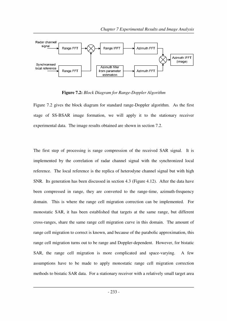
Chapter 7 Experimental Results and Image Analysis
- 233 -
Figure 7.2: Block Diagram for Range-Doppler Algorithm
Figure 7.2 gives the block diagram for standard range-Doppler algorithm. As the first
stage of SS-BSAR image formation, we will apply it to the stationary receiver
experimental data. The image results obtained are shown in section 7.2.
The first step of processing is range compression of the received SAR signal. It is
implemented by the correlation of radar channel signal with the synchronized local
reference. The local reference is the replica of heterodyne channel signal but with high
SNR. Its generation has been discussed in section 4.3 (Figure 4.12). After the data have
been compressed in range, they are converted to the range-time, azimuth-frequency
domain. This is where the range cell migration correction can be implemented. For
monostatic SAR, it has been established that targets at the same range, but different
cross-ranges, share the same range cell migration curve in this domain. The amount of
range cell migration to correct is known, and because of the parabolic approximation, this
range cell migration turns out to be range and Doppler-dependent. However, for bistatic
SAR, the range cell migration is more complicated and space-varying. A few
assumptions have to be made to apply monostatic range cell migration correction
methods to bistatic SAR data. For a stationary receiver with a relatively small target area

Chapter 7 Experimental Results and Image Analysis
- 234 -
and quasi-monostatic topology, an approximation is to consider that the range cell
migration is range-invariant, so that all targets experience the same range cell migration
as the target at the imaging scene centre. In this case, the range cell migration correction
can be implemented by a range FFT, linear phase multiply and range IFFT. This method,
however, imposes a limit on the range interval of observation. After range cell migration
has been corrected, azimuth compression is performed. The principle is the same, but
since the parabolic approximation has been assumed, the equations for the received and
reference azimuth signals should be recalculated. The output of the azimuth compression
yields the complex image of the observation area.
Bistatic Back-Projection Algorithm
In this section a conceptual overview of the generalized bistatic back-projection
algorithm (BBPA) algorithms will be presented. It has been applied to the experimental
data obtained from ground moving and airborne receiver experiments. Two image results
are shown and analyzed in section 7.3, which is from one target area, simultaneously
illuminated by two Galileo satellites.
The bistatic back-projection algorithm operates only partially in the frequency domain,
thus suffering from inefficiency problems. Interestingly, however, it appears that the first
generalized algorithm for bistatic SAR was a modification of the back-projection
algorithm. Its principle of operation is very similar to that of the monostatic back-
projection algorithm, the only difference lying in the calculation of the transmitter-target-

Chapter 7 Experimental Results and Image Analysis
- 235 -
receiver propagation time delay which is used in the interpolation step. A block diagram
of the BBPA is shown in Figure 7.3, followed by appropriate discussion.
Figure 7.3: Block Diagram of BBPA
It can be seen that, conceptually, the BBPA is the same as its monostatic counterpart.
The first step in the algorithm is the standard range compression performed in the range
frequency domain. This step performs the summation over all the available discrete
samples it of equation (7.3). If the range-time match-filtered signal at the grid point
( )RjiR uR ,0 is denoted again by ( )[ ]uuts ijM , , the range compression output is:
( ) ( ) ( ) ( ) ( )( )
, ,, , ,
T i j R i j
i j M M ij
u u
R u R uf R u s u s t u u
c
+ = =
∑ ∑ , (7.10)
then ( )utij in this case is given by:
( ) ( ) ( ) ( )( )uRuRut jiRjiTij ,, += , (7.11)

Chapter 7 Experimental Results and Image Analysis
- 236 -
with ( )( )uR jiT , , ( )( )uR jiR , given by (7.4), (7.5). As in the monostatic case, this means that,
in practice, the discrete fast-time samples of ( )utsM , must be interpolated to
recover ( )[ ]uuts ijM , . The only difference is in the calculation of ( )utij.
If range cell migration exists after range compression, it is seen from (7.10) that the SAR
signal energy is distributed along a number of range bins. However, a corrective process
is suggested and stated explicitly in [1]: “to form the target function at a given grid point,
one could coherently add the data at the fast-time bins that correspond to the location of
that point for all synthetic aperture locations u ” (i.e. execute the azimuth time
summation of (7.10)). In practice, this is done by an interpolation in the range time
domain, so as to recover ( )[ ]uuts ijM , from the discrete fast-time samples of ( )utsM , . The
back-projection algorithm owes its name to this concept. For each aperture position, the
back-projection algorithm traces the range-processed data back (back-projection) in the
range time domain to isolate the return of a reflector at a given point in the image output
grid.
The actual implementation steps, applied the experimental data for bistatic back-
projection algorithm, are the following:
� Fast time domain matched filtering, ( ) ,M
s t u u
� Fast time frequency domain interpolation by zero padding, ( )[ ]uuts ijM ,
� Create the image matrix ( ),i j
f x y with local coordinates

Chapter 7 Experimental Results and Image Analysis
- 237 -
� For fixed ( ),i j
f x y and one azimuth position, find ( )ijt u
� Change the azimuth position, repeat the above step and sum ( ) ,M ij
u
s t u u ∑
The bistatic back-projection algorithm suffers the same inefficiency problems as the
back-projection algorithm. A more efficient version of the bistatic back-projection
algorithm has also been developed [2]. We will briefly describe its main principle. Let us
use the term “projection” to define the location of the target’s cross-correlation function
in fast-time, for a single sampling point in the receiver’s aperture, after range
compression and range time interpolation (according to Figure 7.3). If we have N
samples in the receiver’s aperture, we need to back-project N projections of the target to
reconstruct it. This means that if we have an imaging grid of NxN points, we need to
back-project N projections for each of the N2 pixels, so the total computational cost is N
3.
The efficient version of the bistatic back-projection algorithm states that images that are
half the size of the original image can be reconstructed from half the number of
projections [3].
With this in mind, let us go back to our previous example. Suppose we split our imaging
grid into four sub-images. Each sub-image has N/2xN/2 points. For each pixel in the
sub-image, we only need to back-project N/2 projections. The total computational cost
for each sub-image is now N3/8, and for the whole image it is N
3/2. This means that by
splitting the image into four sub-images, we have reduced the computational cost by a
factor of two. Decomposing the image recursively, and back-projecting using half the

Chapter 7 Experimental Results and Image Analysis
- 238 -
number of projections for the smaller sub-images, the total computational cost reduces
further.
However, there is a problem in using this algorithm when the carrier frequency of the
transmitted signal is high. Even for the standard back-projection algorithm, the range
time interpolator must be accurate enough to recover the samples of ( )[ ]uuts ijM ,
correctly. If the upsampling factor of the interpolator is insufficient, phase errors are
introduced which could be significant. This upsampling factor was found to be
proportional to the carrier frequency of the transmitted signal. This means that as the
carrier frequency increases, our imaging grid at the output of the interpolator must have
more samples in the range time direction. In that case the interpolation step, as well as
the azimuth summation step (in whatever way it is performed), make the back-projection
algorithm and the bistatic back-projection algorithm inefficient.
7.2 Experimental Image Results – Stationary Receiver
This section presents the experiment image results, obtained from stationary receiver
experiments. The data used was collected on 04.11.2009, with GIOVE-A satellite as the
transmitter. One corner reflector (CR) has been used as the reference target at the
distance of 45 m to the stationary receiver. The experimental set-up and other parameters
for the data collection have been included in section 6.2.
The results from two data sets will be introduced below; the two data sets are 30 s and
120 s long (total integration time) respectively. One data set was recorded at 12:56:34

Chapter 7 Experimental Results and Image Analysis
- 239 -
GMT and the other one was recorded at 12:57:55 GMT. The results shown below,
Figures 7.4 and 7.5 include the synchronisation results (delay, Doppler shift and phase
tracking outputs), heterodyne channel focusing results and radar channel azimuth
compressing (imaging) results. Each result will be comprehensively described and
explained.
0 0.5 1 1.5 2 2.5 3
x 104
2.75
2.8
2.85
2.9
2.95x 10
4
Time, ms
Dela
y,
sam
ple
(a) delay
0 500 1000 1500 2000 2500 3000 3500 4000 4500 50001485
1490
1495
1500
1505
1510
1515
1520
1525
Time, 6 ms
Fre
quency,
Hz
before LMS
LMS
(b) Doppler shift
1495 1500 1505 15100
500
1000
1500
2000
2500
3000
3500
Frequency, Hz
Mag
nitud
e
(c) phase history
Figure 7.4: Synchronisation Outputs

Chapter 7 Experimental Results and Image Analysis
- 240 -
Figure 7.4 above shows the synchronisation outputs for the 30 s data set. It includes the
delay tracking output, Doppler tracking output and phase tracking output. These
parameters will be used for the local reference generation for further image formation
processing. The detail of the synchronisation algorithm and local reference generation
has been discussed in Chapter 4. From Figure 7.4(c), the Doppler bandwidth is about
5 Hz for 30 s observation.

Chapter 7 Experimental Results and Image Analysis
- 241 -
Range samples
Azi
muth
posit
ion
s
10 20 30 40 50 60 70 80 90 100
0.5
1
1.5
2
2.5
x 104
(a) Range compression of heterodyne channel data
0 10 20 30 40 50 60 70 80 90 100-45
-40
-35
-30
-25
-20
-15
-10
-5
0
Range samples
Magnitu
de,
dB
(b) Range cross-section
0 0.5 1 1.5 2 2.5 3
x 104
-8
-7
-6
-5
-4
-3
-2
-1
0
Azimuth samples
Magnitu
de,
dB
(c) Azimuth frequency

Chapter 7 Experimental Results and Image Analysis
- 242 -
Range samples
Azi
muth
frq
uency
2 4 6 8 10 12 14 16 18 20
440
460
480
500
520
540
560
(d) FFT of range compression output
495 500 505 510-60
-50
-40
-30
-20
-10
0
Azimuth frequency
Magn
itud
e,
dB
(e) azimuth frequency
Figure 7.5: Heterodyne Channel Range Compression Results
Figure 7.5 above gives the heterodyne channel range compression results. This step is
used to establish whether the local reference signal created after synchronisation and used
for compressing the radar channel data in range is correct. The main concern was
whether the reference signal contains the correct Doppler/phase. For Figure 7.5(a), the
X-axis is the range sample, the first 100 range bins are shown; the Y-axis is the azimuth
sample, 30000 azimuth samples (1ms/sample) are equivalent to 30s azimuth integration
time. It can be seen that data in heterodyne channel were compressed using a reference
signal which contained the tracked signal delay, but not the tracked Doppler/phase. Its
range and cross-range cross-section are given in Figures 7.5(b) and 7.5(c).
At each cross-range position, target energy is concentrated at the first range bin,
indicating that the tracked signal delay is correct. Selecting all samples at this range bin
and taking a Fourier Transform, yields the Doppler spectrum of the heterodyne signal
(Figure 7.5(e)). The result of azimuth FFT on range compression output is shown in

Chapter 7 Experimental Results and Image Analysis
- 243 -
Figure 7.5(d). By comparing Figure 7.5(e) and Figure 7.4 (c), the two phase spectrum are
identical, hence both the local reference generation method and range compression have
been verified. We can then proceed to compress the heterodyne signal in azimuth using
the tracked phase.
Range samples
Azi
muth
posit
ion
s
2 4 6 8 10 12 14 16 18 20
1.3
1.35
1.4
1.45
1.5
1.55
1.6
1.65
1.7
x 104
(a) Focusing of heterodyne data (azimuth compression)
0 10 20 30 40 50 60 70 80 90 100-60
-50
-40
-30
-20
-10
0
Range samples
Magnitu
de,
dB
(b) Range cross-section
1.3 1.35 1.4 1.45 1.5 1.55 1.6 1.65 1.7
x 104
-60
-50
-40
-30
-20
-10
0
Azimuth positions
Magnitu
de,
dB
(c) Cross range cross-section
Figure 7.6: Heterodyne Channel Focusing

Chapter 7 Experimental Results and Image Analysis
- 244 -
Figure 7.6 shows the focusing results of the heterodyne channel data. The tracked phase
(Figure 7.4(c)) is used to form the azimuth filter as discussed previously. It can be seen
that the heterodyne channel has been properly compressed, both in range and in azimuth.
A sinc function, like point spread function, has been obtained (Figure 7.6(a)). The
mainlobe width of the correlation peak in range is equal to 5 range samples,
corresponding the 10 MHz ranging code sampled by 50 MHz. A cross-section of the
compressed output along the azimuth direction is shown in Figure 7.6(c). We can now
proceed to compress the radar channel signal in range and in azimuth.
Range samples
Azi
muth
posit
ion
s
10 20 30 40 50 60 70 80 90 100
0.5
1
1.5
2
2.5
x 104
(a) Range compression of radar channel data

Chapter 7 Experimental Results and Image Analysis
- 245 -
Range samples
Azi
muth
frq
ue
ncy
2 4 6 8 10 12 14 16 18 20
440
460
480
500
520
540
560
(b) azimuth FFT
Range samples
Azi
muth
posit
ion
s
10 20 30 40 50 60 70 80 90 100
0.5
1
1.5
2
2.5
x 104
(c) azimuth compression (imaging)
Figure 7.7: Corner Reflector Imaging Results

Chapter 7 Experimental Results and Image Analysis
- 246 -
Figure 7.7 gives the imaging results from the stationary receiver experiment for corner
reflector detection. It is obtained by compressing the radar channel data using a
simplified range-Doppler algorithm. One critical assumption has been made, which is the
azimuth history of the corner reflector (45 m to receiver) is equal to the phase history
tracked in the heterodyne channel. This is true because the transmitter-to-target range of
23000 km contrasts to the 45 m receiver-to-target range.
Figure 7.7(a) presents the range compression output of radar channel signal. It can be
seen that the SNR is relatively low with no obvious correlation because it is a reflected
signal. However, as soon as an FFT is applied to this output, two frequency spectrums
(Figure 7.7(b)) can be identified in the range time-azimuth frequency domain. Using the
tracked phase as an azimuth filter, the azimuth compression has been formed.
From Figure 7.7(c), we can see that two point target like reflections are clearly shown.
The first point spread function is identified as the direct interference in the radar channel
(compare to Figure 7.6(a)), which is received by the sidelobe of radar channel antenna.
The second point spread function is identified as the reflection from the corner reflector;
it appears at the 14th
range sample, which is equal to the slant range of 84 m to the
receiver. This is because the slant range here is actually the bistatic range, which is the
sum of the receiver-to-target range and the difference between the transmitter-to-target
and the transmitter-to-receiver ranges. In this experimental set-up, it is approximately
twice (90 m) the receive-to-target range, considering the small bistatic angle. The colour

Chapter 7 Experimental Results and Image Analysis
- 247 -
scale of the radar image is in dB, where 0 dB represents the pixel with the highest
intensity. The dynamic range of the image has been artificially clipped to 30 dB.
Range samples
Azi
muth
posit
ion
s
2 4 6 8 10 12 14 16 18 20
1.3
1.35
1.4
1.45
1.5
1.55
1.6
1.65
1.7
x 104
(a) zoom (corner reflector image )
0 10 20 30 40 50 60 70 80 90 100-60
-50
-40
-30
-20
-10
0
Range samples
Magnitu
de,
dB
(b) Range cross-section
1.3 1.35 1.4 1.45 1.5 1.55 1.6 1.65 1.7
x 104
-60
-50
-40
-30
-20
-10
0
Azimuth positions
Magnitu
de,
dB
(c) Cross range cross-section
Figure 7.8: Corner Reflector Imaging Results
Figure 7.8 presents the zoom plot of corner reflector image with its cross-sections.

Chapter 7 Experimental Results and Image Analysis
- 248 -
0 0.5 1 1.5 2 2.5 3
x 104
1490
1500
1510
1520
1530
1540
1550
1560
1570
Time, 6 ms
Fre
quenc
y,
Hz
before LMS
LMS
(a) Doppler shift
1500 1510 1520 1530 1540 1550 15600
500
1000
1500
2000
2500
3000
3500
Frequency, Hz
Magn
itud
e
(b) phase history
Figure 7.9: Synchronisation Outputs
Figure 7.9 above shows the synchronisation outputs for the 120 s data set. From Figure
7.9(b), the Doppler bandwidth is about 25 Hz for 120 s observation. We should expect
the improvement in azimuth resolution for this data, comparing to the 30 s data.
Range samples
Azi
muth
posit
ion
s
10 20 30 40 50 60 70 80 90 100
2
4
6
8
10
12
x 104
(a) azimuth compression output (imaging)

Chapter 7 Experimental Results and Image Analysis
- 249 -
Range samples
Azi
muth
posit
ion
s
2 4 6 8 10 12 14 16 18 20
5.8
5.85
5.9
5.95
6
6.05
6.1
6.15
6.2
x 104
(b) zoom (corner reflector image )
Figure 7.10: Corner Reflector Imaging Result 2
With the same processing procedures applied to 120 s data, Figure 7.10 gives another
imaging result from the stationary receiver experiment for corner reflector detection. Y-
axis of Figure 7.10(a) indicates 120000 azimuth positions this time. Again, we can see
that two point target like reflections are clearly shown. The second point spread function
appears at the 14th
range sample too, which is equal to the slant range of 84 m to the
receiver. The colour scale of the radar image is in dB, where 0 dB represents the pixel
with the highest intensity. The dynamic range of the image has been artificially clipped
to 30 dB.

Chapter 7 Experimental Results and Image Analysis
- 250 -
Figure 7.11 below shows the range and cross-range cross-sections of second point spread
function of both images (30 s and 120 s). It is clearly seen that SNR has improved and
finer azimuth resolution has been achieved by using a longer integration time.
0 10 20 30 40 50 60 70 80 90 100-60
-50
-40
-30
-20
-10
0
Range samples
Mag
nitud
e,
dB
30 s
120 s
(a) Range cross-section
-1000 -800 -600 -400 -200 0 200 400 600 800 1000-60
-50
-40
-30
-20
-10
0
Azimuth positions
Magn
itu
de,
dB
30 s
120 s
(b) Cross range cross-section
Figure 7.11: Range and Cross Range Cross-sections

Chapter 7 Experimental Results and Image Analysis
- 251 -
7.3 Experimental Image Results – Ground Moving Receiver
This section presents the experiment image results, obtained from the ground moving
receiver experiments. The data used was collected on 22.12.2008, with both GIOVE-A
and GIOVE-B satellites signals received. The experimental set-up and other parameters,
such as the target area analysis, have been included in section 6.3. The separated houses
shown in Figure 6.10 are used as the targets for detection.
Galileo satellites adopt a CDMA scheme; one recorded data set can contain the signals
from all visible satellites. So, two images can be generated with one receiver aperture
from both GIOVE A/B satellites. The two image results will be introduced below; the
data length is 30 s and it was recorded at 10:18:18 GMT. The results shown below
include heterodyne channel focusing results and radar channel azimuth compressing
(imaging) results. The description and explanation of each result will be
comprehensively discussed.
To implement the full bistatic back-projection algorithm described in section 7.1, we also
need to verify whether the instantaneous ranges (transmitter-target, receiver-target and
transmitter-receiver) calculated from our extracted transmitter and receiver positions are
correct. The parameter estimation results are included and discussed in section 6.5.4 for
this particular data.

Chapter 7 Experimental Results and Image Analysis
- 252 -
Range samples
Azi
muth
frq
ue
ncy
1 2 3 4 5 6 7 8 9 10
640
641
642
643
644
645
646
647
648
649
650
(a) FFT output of range compression for heterodyne data
640 641 642 643 644 645 646 647 648 649 6500
0.1
0.2
0.3
0.4
0.5
0.6
0.7
0.8
0.9
1
Azimuth frequency
Mag
nitu
de,
dB
(b) azimuth frequency cross-section
640 642 644 646 648 6500
0.1
0.2
0.3
0.4
0.5
0.6
0.7
0.8
0.9
1
Frequncy, Hz
Mag
nitu
de
synchronisation
compensated
(c) tracked and compensated phase spectrum
Figure 7.12: Heterodyne Channel Range Compression Results
Figure 7.12 presents the range compression output of the radar channel signal. Following
the same procedures used for the stationary receiver data, the result of azimuth FFT of
range compression output is shown in Figure 7.12(a). By comparing Figure 7.12(b) and
Figure 6.27(d) (repeated here in Figure 7.12(c)), the tracked phase spectrum and azimuth

Chapter 7 Experimental Results and Image Analysis
- 253 -
frequency of FFT output are identical, hence both local reference generation method and
range compression have been verified. We can then proceed to compress the heterodyne
signal in azimuth using the tracked phase.
Range samples
Azi
muth
posit
ion
s
2 4 6 8 10 12 14 16 18 20
0.5
1
1.5
2
2.5
3
x 104
(a) Focusing of heterodyne data (azimuth compression)
0 10 20 30 40 50 60 70 80 90 100-60
-50
-40
-30
-20
-10
0
Range samples
Mag
nitu
de,
dB
(b) Range cross-section
0.5 1 1.5 2 2.5 3
x 104
-60
-50
-40
-30
-20
-10
0
Azimuth positions
Mag
nitu
de,
dB
(c) Cross range cross-section
Figure 7.13: Heterodyne Channel Focusing
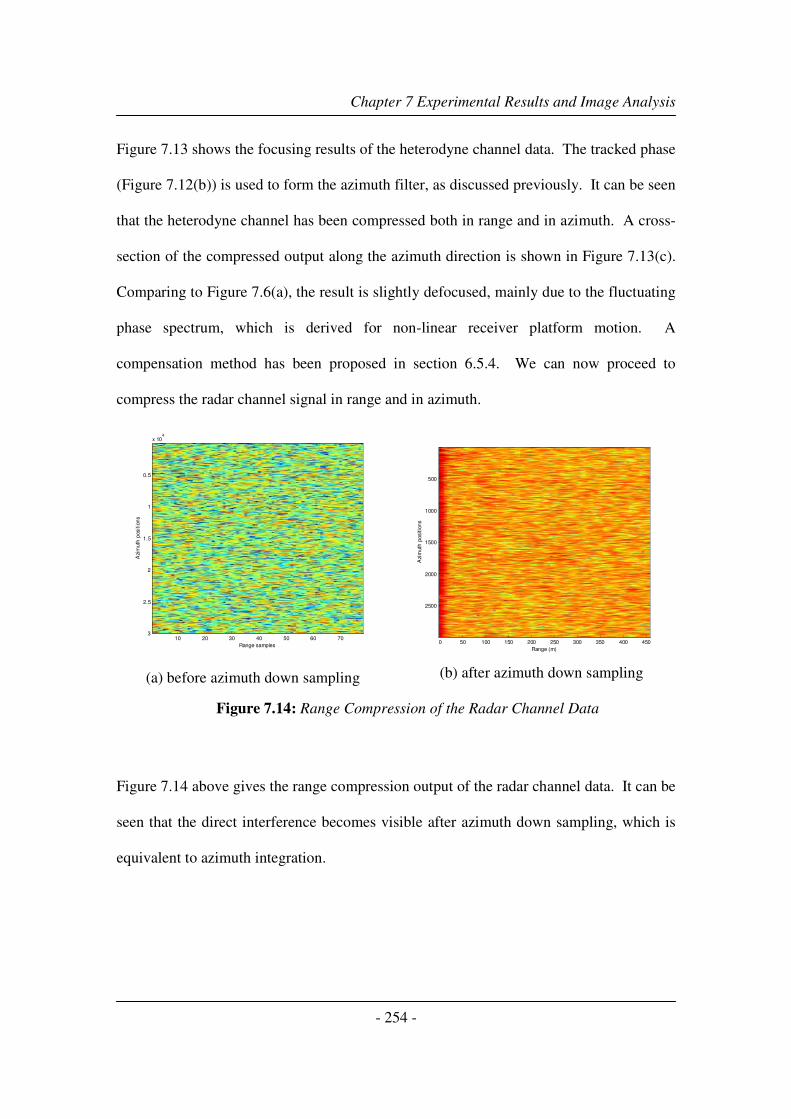
Chapter 7 Experimental Results and Image Analysis
- 254 -
Figure 7.13 shows the focusing results of the heterodyne channel data. The tracked phase
(Figure 7.12(b)) is used to form the azimuth filter, as discussed previously. It can be seen
that the heterodyne channel has been compressed both in range and in azimuth. A cross-
section of the compressed output along the azimuth direction is shown in Figure 7.13(c).
Comparing to Figure 7.6(a), the result is slightly defocused, mainly due to the fluctuating
phase spectrum, which is derived for non-linear receiver platform motion. A
compensation method has been proposed in section 6.5.4. We can now proceed to
compress the radar channel signal in range and in azimuth.
Range samples
Azi
muth
posi
tion
s
10 20 30 40 50 60 70
0.5
1
1.5
2
2.5
3
x 104
(a) before azimuth down sampling
Range (m)
Azi
muth
posi
tion
s
0 50 100 150 200 250 300 350 400 450
500
1000
1500
2000
2500
(b) after azimuth down sampling
Figure 7.14: Range Compression of the Radar Channel Data
Figure 7.14 above gives the range compression output of the radar channel data. It can be
seen that the direct interference becomes visible after azimuth down sampling, which is
equivalent to azimuth integration.

Chapter 7 Experimental Results and Image Analysis
- 255 -
Figure 7.15 below shows the interpolation results after range compression. For this data,
50 times interpolation has been applied and range cross-section remains the same.
0 10 20 30 40 50 60 70 800
20
40
60
80
100
120
140
160
Range samples
Mag
nitu
de
(a) Before range sample interpolation
0 500 1000 1500 2000 2500 3000 3500 40000
20
40
60
80
100
120
140
160
180
Range samples
Mag
nitu
de
(b) After range sample interpolation
Figure 7.15: Range Interpolation Results

Chapter 7 Experimental Results and Image Analysis
- 256 -
Range pixels
Azi
muth
pix
els
5 10 15 20 25 30 35 40 45 50
10
20
30
40
50
60
70
80
90
100
1000
2000
3000
4000
5000
6000
Figure 7.16: Moving Receiver Imaging Result – GIOVE A
A SAR intensity image using GIOVE-A satellite is shown in Figure 7.16. The Radar
image covers the target area of 300 m x ~180 m, with pixel size 6 m x 1.8 m. The
satellite photograph of the target area is shown in Figure 7.17. The receiver was mounted
on a ground vehicle, moving along the road on the left in the figure. As can be seen in
Figure 7.17, the dominant target is an extended structure towards the middle of the scene
(at a range of approximately 250 m). From Figure 7.16, it can be seen that some strong
reflections have been detected. Moreover, buildings on the centre and upper side of the
imaging area are visible. The area surrounding these buildings is grassland and therefore

Chapter 7 Experimental Results and Image Analysis
- 257 -
its intensity is lower. Parts of the forested area towards the site of the building can also
be seen.
Figure 7.17: Target Area – Separated Houses

Chapter 7 Experimental Results and Image Analysis
- 258 -
Range pixels
Azi
muth
pix
els
5 10 15 20 25 30 35 40 45 50
10
20
30
40
50
60
70
80
90
100
1000
2000
3000
4000
5000
6000
7000
Figure 7.18: Moving Receiver Imaging Result – GIOVE B
Figure 7.18 presents the image result from the same data, but using the GIOVE-B
satellite. Due to a different bistatic angle, the reflection properties of the target area are
changed. Hence the image obtained is slightly different to the one from GIVOE-A.
At the moment, there are a few factors affecting image quality. One is the accuracy of
the satellite positions, which introduces errors in the calculated instantaneous bistatic
range; the other is the output of the synchronisation algorithm. The tracked Doppler of
the direct transmitter-receiver signal contains a contribution from receiver motion errors,
but this amount is unknown (due to the fact that a least-mean square algorithm is applied

Chapter 7 Experimental Results and Image Analysis
- 259 -
to get an average estimate). Since this tracked Doppler is mixed with the transmitter-
target-receiver Doppler, the mixed signal (and hence the final image product) contains
motion errors too.
It is possible that the above factors are responsible for limiting the quality of the image in
terms of contrast and proper focus. These limitations can only be overcome through step-
by-step verification of the image formation algorithm, perhaps adding some
modifications to it (e.g. an autofocus technique). Even so, it appears that an intensity
image has been obtained which corresponds to the reflectivity of the inspected terrain.
Even though the radar reflectivity map can be associated with features of the imaging
area, it was clear that there was a lot of room for improvement.
7.4 Summary
In this chapter, the structure of the BSAR collected data are described to provide a brief
background of general methods used for SAR signal compression. Conceptual
descriptions of two BSAR image formation algorithms are provided, which have been
applied to the experimental data. The range-Doppler algorithm (RDA) has been applied
to the experimental data and collected for the stationary receiver experiment. The image
results are included in section 7.2, for a corner reflector detection. The reason for this is
the simplicity of its implementation; the experimental topology is quasi-monostatic with
small bistatic angle. The generalized bistatic back-projection algorithm (BBPA)

Chapter 7 Experimental Results and Image Analysis
- 260 -
algorithms have been applied to the experimental data obtained from the ground moving
and airborne receiver experiments. Two image results are shown and analyzed in section
7.3, which is from one target area, simultaneously illuminated by two Galileo satellites.
Reference
1. Soumekh, M., Synthetic Aperture Radar signal processing with Matlab algorithms.
1999: Wiley-Interscience.
2. Ding, Y., Synthetic Aperture Radar image formation for the moving-target and
near-field bistatic cases. 2002.
3. Ding, Y. and D.C. Munson, A fast back-projection algorithm for bistatic SAR
imaging, IEEE ICIP, 2002. 2: p. II-449 - II-452.

Chapter 8 Conclusions and Future Work
- 261 -
Chapter 8 Conclusions and Future Work
8.1 Conclusions
This thesis focuses on SS-BSAR using GNSS as the transmitter of opportunity. The
main goal of this research is to investigate the feasibility of a BSAR system using
spaceborne navigation satellites and verify its performance, such as spatial resolution and
signal-to-noise ratio (SNR). Both stationary and moving receivers have been considered,
and Galileo satellites have been used as the non-cooperative transmitter for the
experimentation.
First of all, the proposed SS-BSAR system has been theoretically analysed for system
parameters, such as the transmitter power, spatial resolution, power budget and the
properties of the ranging signals. It is highlighted that the GNSS satellites transmit 10 dB
less power compared to other satellites, such as TV broadcast vehicles. However, it has
an advantage of satellite diversity and thus one can choose the desired bistatic topology
for low resolution loss. It is concluded that overall a GNSS satellite is the most suitable,
non-cooperative transmitter candidate for SS-BSAR. It provides a reasonable range
resolution of ~ 8-15 m and a target detection range of ~ 3-12 km for 50 m2 targets.
The most promising GNSS for the considered purpose are the EU Galileo satellites and
the new GPS III satellites. These satellites can potentially provide a range resolution of
about 8 m against 30 m for GLONASS. The Galileo E5 and new GPS L5 signals also

Chapter 8 Conclusions and Future Work
- 262 -
provide at least 6 dB more received power compared to the GLONASS L1 channel.
Therefore one can expect a four times improvement in the maximum operational range.
As GNSS signals are designed for navigation purposes, one navigation signal (Galileo
E5) has been studied analytically, in terms of radar applications. Its signal correlation
property has been investigated by simulation and a technique has been simulated to
combine the full E5 bandwidth and potentially improve the range resolution for a GNSS
based SS-BSAR system.
Synchronisation, as an inevitable issue for a non-cooperative bistatic system, has also
been investigated. In our case, phase synchronisation is the most important as the largely
separated transmitter and receiver must be coherent over extremely long intervals of time.
Synchronisation using a direct link signal has been proposed and the algorithm to extract
the required information has been applied to the experimental data. The synchronisation
experiment confirmed that a minimum 10 dB SNR is required in the heterodyne channel.
To obtain the experimental data for image formation and confirm the system analysis
results, an experimental test bed for the proposed SS-BSAR system has been developed
and tested with full functionality. Experimentation methodology has been planned and a
number of experiments have been conducted, such as a synchronisation experiment, a
stationary receiver experiment, a ground moving receiver experiment and an airborne
receiver experiment. A set of data has been collected for radar imaging. To generate a
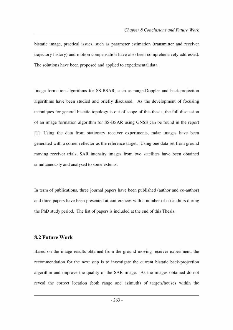
Chapter 8 Conclusions and Future Work
- 263 -
bistatic image, practical issues, such as parameter estimation (transmitter and receiver
trajectory history) and motion compensation have also been comprehensively addressed.
The solutions have been proposed and applied to experimental data.
Image formation algorithms for SS-BSAR, such as range-Doppler and back-projection
algorithms have been studied and briefly discussed. As the development of focusing
techniques for general bistatic topology is out of scope of this thesis, the full discussion
of an image formation algorithm for SS-BSAR using GNSS can be found in the report
[1]. Using the data from stationary receiver experiments, radar images have been
generated with a corner reflector as the reference target. Using one data set from ground
moving receiver trials, SAR intensity images from two satellites have been obtained
simultaneously and analysed to some extents.
In term of publications, three journal papers have been published (author and co-author)
and three papers have been presented at conferences with a number of co-authors during
the PhD study period. The list of papers is included at the end of this Thesis.
8.2 Future Work
Based on the image results obtained from the ground moving receiver experiment, the
recommendation for the next step is to investigate the current bistatic back-projection
algorithm and improve the quality of the SAR image. As the images obtained do not
reveal the correct location (both range and azimuth) of targets/houses within the

Chapter 8 Conclusions and Future Work
- 264 -
observation area, the possible causes should be examined. Except for faults in the image
formation algorithm itself, other causes could be due to errors in estimated satellite
positions or otherwise due to errors from the synchronisation outputs.
Moreover, the development of a frequency domain general BSAR image formation
algorithm should be considered, as a bistatic back-projection algorithm lacks efficiency
while processing airborne data from large target area.
Figure 8.1: Future of GNSS based SS-BSAR
A few minor issues are also worth further analysis. One is the range resolution
improvement by combining GNSS bandwidth. Answers need to be considered regarding
how to apply the proposed method during the image formation process. Experimental

Chapter 8 Conclusions and Future Work
- 265 -
data may be collected to verify the simulation results shown in Chapter 3. The other
problem is the motion compensation for SS-BSAR general topology, particularly for an
airborne receiver platform. The current solution may be improved by applying data
fusion to GPS and inertial navigation outputs.
Finally, Figure 8.1 gives an artistic view for the future of a GNSS based SS-BSAR
system. With over 100 navigation satellites available in 10 years time and the inbuilt
advantage of optimal bistatic topology and easy synchronisation, such systems have
excellent potential for advanced SAR applications, such as polarimetric and
interferometric image generation. Power integration from multiple satellites is also
possible to improve the system power budget, which is the main disadvantage of such a
system. Employing ultra low cost commercial GNSS receiver hardware, GNSS based
SS-BSAR will be a viable and important solution for many remote sensing applications.
Reference
1. Cherniakov, M., et al., Bistatic Synthetic Aperture Radar with Emitters of
Opportunity. 2006, Unversity of Birmingham: Birmingham.

Appendixes A to H
- 266 -
Appendix A Galileo Spreading Codes Generation
The spreading codes for a Galileo E5 signal consist of a primary spreading code and a
secondary code used for pilots and for signals with low data rate. The secondary code is
used to modulate the primary code like a deterministic data modulation, to generate a total
code length that is a multiple of the primary code length. With GIOVE-A and GIOVE-B,
the primary spreading codes are generated as truncated combined M-sequences (maximum
length sequence) that can be implemented using linear feedback shift register (LFSR)
techniques. Secondary codes are short-memory stored pseudo random sequences. The
code length to be used for each of the E5 signal components is the value stated in the table
below.
Table A-1: Spreading code lengths for GIOVE-A and GIOVE-B
Code Length (chips) Channel Chip Rate
(Mcps)
Code Length
(ms) Primary Secondary
Symbol
Rate (sps)
E5a-I 10.23 20 10230 20 50
E5a-Q 10.23 100 10230 100 No
E5b-I 10.23 4 10230 4 250
E5b-Q 10.23 100 10230 100 No
A.1 Spreading Codes Generation
The Galileo E5 primary spreading codes are generated by a tiered code construction.
Register based primary codes used in Galileo are generated as combinations of two M-
sequences, being truncated to the appropriate length, whereby a secondary code sequence
is used to modify successive repetitions of a primary code. When considering a primary
code with length N chips and an associated secondary code with length Ns chips, the first

Appendixes A to H
- 267 -
chip of the secondary code in binary representation is used to control the polarity of the
first epoch of the primary code sequence by exclusive-or combination, as shown in Figure
A1 below. If applicable, data modulation is applied to the full code, again using the
exclusive-or combination of code and data symbols.
Primary
CodeClock
Secondary
Code/N
XOR
Clock rate fc
fc
fcs
Primary code length NSecondary code length Ns
Primary code chiprate fcSecondary code chiprate fcs=fc/N
Spreading
Code
Figure A.1: Code construction principle
A.2 Primary Codes
Figure A2 below shows an example implementation of the linear feedback shift register
method for generation of truncated and combined M sequences for the E5a-I signal.
Figure A.2: Linear shift register based code generator

Appendixes A to H
- 268 -
Two parallel registers are used: base register 1 and base register 2. The primary output
sequence is the exclusive OR of register 1 and 2 outputs; the shift between the two
sequences is zero. For truncation to primary code-length N, the content of the two shift
registers is reinitialized after N cycles of the registers with so-called start-values. The start
values for all base register 1 cells, in logic level notation, are “1” for all codes. The start
values for all base register 2 cells are defined in Galileo Signal In Space Interface Control
Document [1]. The E5a-I, E5a-Q, E5b-I and E5b-Q primary codes apply same principle,
using the parameters defined in Table below.
Table A-2: Primary code parameters
Signal Register Feedback Taps Register
Length
Start Values
Base 1 1, 6, 8, 14 14 All “1” E5a-I
Base 2 4, 5, 7, 8, 12, 14 14 From specification
Base 1 1, 6, 8, 14 14 All “1” E5a-Q
Base 2 4, 5, 7, 8, 12, 14 14 From specification
Base 1 4, 11, 13, 14 14 All “1” E5b-I
Base 2 2, 5, 8, 9, 12, 14 14 From specification
Base 1 4, 11, 13, 14 14 All “1” E5b-Q
Base 2 1, 5, 6, 9, 10, 14 14 From specification
A.3 Secondary Codes
The secondary codes are fixed sequences with length defined in Table A-1 and more
details can be found in the Galileo Signal In Space Interface Control Document [1]. For
the 4 and 20 bit secondary codes the same code is used for all associated primary codes.
For the 100 bit code, an independent secondary code is assigned for each primary code.

Appendixes A to H
- 269 -
Appendix B Coordinate and Datum Transformations
Coordinate transformations are used to convert from one type of coordinates to another
type of coordinates. Datum transformations are used to convert between a global
coordinate and a local coordinate system. A geodetic datum defines the relationship
between a global and a local three-dimensional Cartesian coordinate system. With both
the transformations, we can convert the earth ellipsoids coordinates to target ellipsoids
coordinates.
Two different coordinate systems are most commonly used to represent the earth
ellipsoids: Cartesian coordinates (x, y and z) and geographic LLA coordinates (Latitude,
Longitude and Altitude), which is a global coordinate system. Coordinate transformations
can be applied to convert a global Latitude Longitude and Altitude coordinates to a global
XYZ coordinates. With known coordinates of at least three points in both systems, a
global Cartesian coordinates can be transferred to a local Cartesian coordinates using 7-
parameters transformation, or called 3D similarity transformation.
B.1 Geographic – Cartesian (La, Lo, A) – (X, Y, Z)
One uses the formula
2
( ) cos cos
( )cos sin
( (1 ) )sin
X N H La Lo
Y N H La Lo
Z N e H La
= +
= +
= − +
with La and Lo are Latitude and Longitude, H being the altitude and N being
2
2 2 2 2 2 21 sin cos sin
a aN
e La a La b La= =
− +

Appendixes A to H
- 270 -
a, b are semi major and semi minor axes of the ellipsoid and e is the eccentricity of the
earth.
B.2 7-parameters transformation
Given the three-dimensional of a point P in a Cartesian coordinate frame (u, v, w), the
coordinates of this point in a different Cartesian coordinates frame (x, y, z) can be
computed using the relation
( )
1
1 1
1P P
x x w u
y y s w v
z z w
δ δϕ
δ δ δε
δϕ δε
−
= + + − ⋅ −
�
�
�
with x� , y� , z� : coordinates of the origin of frame (u, v, w) in frame (x, y, z);
δε , δϕ , wδ : differential rotations around the axes (u, v, w), respectively to
establish parallelism with frame (x, y, z);
sδ : differential scale change.
Considering WGS84 or ITRF to be the (u, v, w) frame and local coordinates to be (x, y, z)
frame, coordinates of a Galileo satellite or radar receiver platform can be transformed to
local coordinates, once these seven transformation parameters are know.

Appendixes A to H
- 271 -
Appendix C Antennas and Front-end
C.1 Spiral Helix Antennas
Table C-1: Spiral Helix Antenna Parameters
-40
-35
-30
-25
-20
-15
-10
-5
0
5
10
15
20
-180 -150 -120 -90 -60 -30 0 30 60 90 120 150 180
Angl e ( de gr e e s)
Co-Polar
X-Polar
Model AMH16-16R-
D2/082
Meas Plane Elevation
Peak Gain 15.5 dBiC
-40
-35
-30
-25
-20
-15
-10
-5
0
5
10
15
20
-180 -150 -120 -90 -60 -30 0 30 60 90 120 150 180
Angl e ( degr ees)
Co-Polar
X-Polar
Model AMH16-16R-
D2/082
Meas Plane Azimuth
Peak Gain 15.5 dBiC
Figure C.1: Radiation Pattern of Spiral Helix Antennas
Model Number Frequency
(GHz)
Gain
(dBi)
HPBW
Az x El
Polarization Dimension
(mm)
Connector
AMH16-16L-02 1.1-1.7 16 30o x 30
o Left Hand
Circular
1005 x 55 N-type (F)
AMH16-16R-02 1.1-1.7 16 30o x 30
o Right Hand
Circular
1005 x 55 N-type (F)

Appendixes A to H
- 272 -
C.2 Flat PCB Patch Antennas
C.2.1 Heterodyne Channel Antenna
Specification
1) Working frequency 1192±25 MHz
2) Working polarization – right circular polarisation, additional polarization – left
circular polarisation
3) Radome dimensions 260х260х25 mm
Antenna concept
The antenna (Figure C2 below) consists of two PCBs. The first single layer PCB is a
quadrant radiating element (patch). The second double-layer PCB has a 90-degree power
splitter for antenna feeding.
Figure C.2: Heterodyne channel antenna concept
The coupler’s PCB2 is installed on a duralumin ground plate. Both PCBs are separated by
5 M3x10 mm spacers and screwed by M3 screws. Two feeding wires (1 mm copper)
connect the coupler and patch being soldered to them. The total assembly of the antenna
PCB2 with hybrid coupler
Radome
PCB1 with patch
RCP input
LCP input

Appendixes A to H
- 273 -
is shown in the drawings Figure C.7. The antenna has two feeding points for right circular
polarisation and left circular polarisation separately. The input connectors are SMA-type.
The connectors unused must be loaded by a 50 Ohm standard SMA load. The Radome is
attached to ground plate by 3x10 wood screws.
Calculated antenna parameters (for 6.4=ε ):
Frequency, MHz Gain, Left Circular
Polarisation, dB
Gain, Right Circular
Polarisation, dB
Axial ratio,
dB
1167 -4.81 9.14 -0.584
1192 -3.47 9.18 -0.076
1217 -2.4 9.22 -0.151
Beam width (at 1192 MHz) is around 65ох66
о.
Antenna bandwidth is 1.11-1.28 GHz (14.2%) at the VSWR=1.5 level.
Simulated antenna parameters are shown in Figures C3, C4 and C5 below.
Figure C.3: Return loss, S11

Appendixes A to H
- 274 -
Figure C.4: Impedance
Figure C.5: VSWR
The drawings of PCBs with dimensions are shown in Figure C6 and C7 below.

Appendixes A to H
- 275 -
130
R30
d1.32X (PCB1)
100
120
d3,2
5X
130
d1.34X
12,2
60
d2,7
4X
d3,2
B
C
D
W R1.25
A
Figure C.6: Antenna PCB layout
PCB1 (one-side copper FR-4-0.8mm)
PCB size 130x130 mm
Patch size 100x100mm
PCB2 (two-side copper FR-4-0.8. One side – top – power splitter, other side – all ground)
Dimension
(mm)
Variant 1 Variant2
A 35.6 33.5
B 32.4 30.5
C 37.7 35.6
D 32.3 30.4
W 1.6 1.5
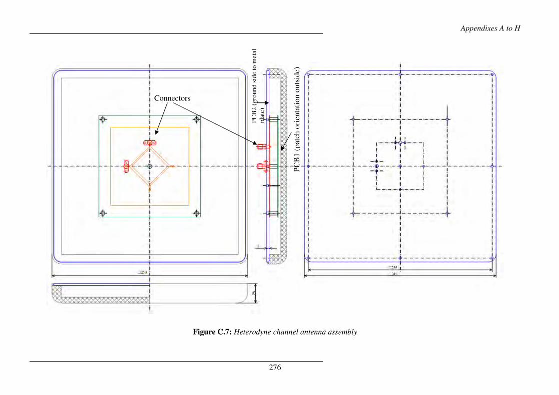
Appendixes A to H
276
Figure C.7: Heterodyne channel antenna assembly
PC
B2
(g
roun
d s
ide
to m
etal
pla
te)
PC
B1 (
pat
ch o
rien
tati
on
outs
ide)
Connectors

Appendixes A to H
277
C.2.2 Radar Channel Antenna
The radar channel antenna used for the vehicle and the airborne trials is a four-
element patch antenna. The design and specifications for each element are the same
as the single element patch antenna used for the heterodyne channel.
Specification
1) Working frequency 1192±25 MHz
2) Working polarization – right circular polarisation, additional polarization – left
circular polarisation
3) Beam width at 1192 MHz around 65ох15
о.
4) Radome dimensions 1000х250х30 mm
Figure C.8: Radar channel antenna concept
Power splitter 1
LHCP output
Power splitter 2
RHCP output
� Estimated parameters: � Gain: 14 dB � Cross-polarization: -14 dB

Appendixes A to H
278
C.2.3 Patch Antennas Testing Results
A set of experiments have been conducted in open space to measure the gain and the
beamwidth of the heterodyne and the radar channel antennas. Figures C.9 and C.11
below show the experimental set-up for the antenna testing. In order to measure the
heterodyne channel antenna gain, S21 measurement has been made using a network
analyzer. Two identical patch antennas were installed with the separation distance of
7 meters, one for transmission and the other for reception.
Figure C.9: Heterodyne channel antenna testing set-up
The calibration of the Network Analyser and connecting cables was conducted and
the input power level was adjusted to set the measured total transmission link gain
(propagation loss, antenna gain, losses from cables etc) to 0 dB. Figure C10 below
show the testing results (S-parameters). Assuming a free space propagation loss
model, the antenna gain is about 7.5 dB and close to the expected value of 9.18 dB at
1192 MHz.
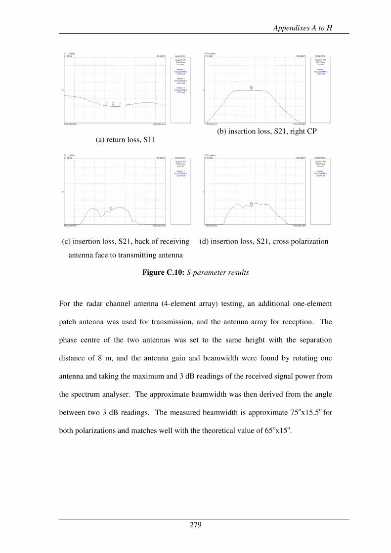
Appendixes A to H
279
(a) return loss, S11 (b) insertion loss, S21, right CP
(c) insertion loss, S21, back of receiving
antenna face to transmitting antenna
(d) insertion loss, S21, cross polarization
Figure C.10: S-parameter results
For the radar channel antenna (4-element array) testing, an additional one-element
patch antenna was used for transmission, and the antenna array for reception. The
phase centre of the two antennas was set to the same height with the separation
distance of 8 m, and the antenna gain and beamwidth were found by rotating one
antenna and taking the maximum and 3 dB readings of the received signal power from
the spectrum analyser. The approximate beamwidth was then derived from the angle
between two 3 dB readings. The measured beamwidth is approximate 75ох15.5
о for
both polarizations and matches well with the theoretical value of 65ох15
о.
Appendixes A to H
280
Figure C.11: Radar channel antenna testing set-up
C.3 GPS Antenna
The PG-A1 is a precision dual-frequency, dual-constellation antenna featuring an
integrated ground plane to help eliminate errors caused by multipath. The PG-A1 was
designed to accompany the Topcon modular receivers such as the Legacy-E, Legacy-
H and Odyssey-RS.
Table C-2: PG-A1 Specifications
Frequency GPS & GLONASS L1/L2
Gain 6 dBi, Omi-directional
Integrated UHF No
Centering Precision Micro Centre
Type Microstrip on flat ground plane
Weight 492 g
Dimensions 141.6mm × 141.6mm × 52.7mm
DC voltage +2.7 ~ +12 V; 25A @ 5.0 typ
LNA gain 30 ± 2 dB

Appendixes A to H
281
Output 50 Ohm
Connector TNC
Environmental Waterproof
Operating temperature -40°C~ +55°C
Shock Resistance 2-meter pole drop
C.4 RF Front-ends
An RF front-end, compatible with the Galileo E5 signals and the antennas described
previously, has been developed. It has two variants; one consists of a first stage low
noise amplifier (noise figure 1.15 dB), RF bandpass filter and 2nd
stage amplifier, the
other only has a first LNA and a RF bandpass filter. Figure C12 below show the
testing results for the front-end blocks developed. The total gain of the front-ends is
around 44 dB for 1st variant and 22 dB for 2
nd variant.
(a) input return loss, S11, block 1 (b) insertion loss, S21, block 1

Appendixes A to H
282
(c) output return loss, S22, block 1 (d) input return loss, S11, block 2
(e) insertion loss, S21, block 2 (f) output return loss, S22, block 2
Figure C.12: Front-end S-parameters results

Appendixes A to H
283
Appendix D Frequency Synthesizer
LMDP_1500_0500_01
1. PRODUCT DESCRIPTION
The LMDP_1500_0500_01 is a small step size frequency synthesizer, which
generates frequencies from 1000MHz to 2000MHz with less than 2.4 Hz resolution
via 31 parallel data bits. The output signal is phase-locked to an internal 10 MHz
TCXO with +/- 1ppm accuracy or an external 10 MHz reference. When an
external 10 MHz reference (+1dBm min.) is applied to J1, the TCXO will be shut-
off automatically and the output signal will be locked to the external reference.
2. SPECIFICATIONS
ELECTRICAL
Main Output (J4)
Frequency Range: 1000 MHz to 2000 MHz
Frequency Resolution: 2.3283 Hz
Frequency Accuracy: Depending on the 10 MHz reference
with an additional error of +/- 2.3283 Hz
Output Power: +13 dBm +/-3 dB
Harmonic: <-20 dBc
Spurious: -45 dBc Typical.
SSB Phase Noise (Fout = 100 MHz, Internal 10 MHz)
@ 1 kHz Offset -80 dBc/Hz
@ 10 kHz Offset -90 dBc/Hz
Internal Reference:
Frequency: 10 MHz
Frequency Stability: +/- 1 ppm
External Reference (J1):
Frequency: 10 MHz
Input Power: +1 dBm minimum
Auxiliary Output (J2):

Appendixes A to H
284
Frequency: 10 MHz Buffered from Int. or Ext. Ref.
Output Power: +3 dBm minimum
DC Input (JP1)
+5 VDC @ 900 mA typ. (1 A Max.)
+15 VDC @ 75 mA typ. (120 mA Max.)
LMDD_LF_300_01
1. PRODUCT DESCRIPTION
The LMDD_LF_300_01 is a direct digital synthesizer (DDS), which generates
frequencies from 500 kHz to 300 MHz in less than 2.4 Hz resolution via 31 parallel
data bits. The unit has a built-in 1 GHz clock. The 1 GHz clock is phase-locked to
an internal 10 MHz TCXO with +/- 1ppm accuracy or an external 10 MHz
reference. When an external 10 MHz reference (+1 dBm min.) is applied to J1, the
TCXO will be shut-off automatically and the 1 GHz clock will be locked to the
external reference.
2. SPECIFICATIONS
ELECTRICAL
Main Output (J4)
Frequency Range: 500 kHz to 300 MHz
Frequency Resolution: .23283 Hz
Frequency Accuracy: Depended on the 10 MHz reference with
an additional error of +/- 0.23283 Hz
Output Power: +6 dBm +/-3 dB
Harmonic: <-20 dBc
Spurious: -45 dBc Typical.
SSB Phase Noise (Fout = 100 MHz, Internal 10 MHz)
@ 1 kHz Offset -105 dBc/Hz
@ 10 kHz Offset -115 dBc/Hz
Internal Reference:

Appendixes A to H
285
Frequency: 10 MHz
Frequency Stability: +/- 1 ppm
External Reference (J1):
Frequency: 10 MHz
Input Power: +1 dBm minimum
Auxiliary Output (J2):
Frequency: 10 MHz Buffered from Int. or Ext. Ref.
Output Power: +3 dBm minimum
DC Input (JP1) +5 VDC @ 800 mA typ. (1 A Max.)
Testing Results and Frequency Setting
Figure D1 below shows the signal spectrum after programming the frequency
synthesizer to the required frequency. For the Galileo receiver, the intermediate
frequency is set to 140 MHz and the RF input is mixed with local frequency of
1347.14 MHz. The next page also gives the circuit diagram for the frequency
programming board.
(a) 140 MHz, IF local frequency

Appendixes A to H
286
(b) 1347.14 MHz, RF local frequency
Figure D.1: Frequency synthesizers output
Figure D2 below shows the PCB diagram of frequency synthesizer setting board. It
has 32 switches, controlling the 0-31 parallel data inputs (TTL high or low) to the
frequency synthesiser. Extra circuitry is also included to indicate the status of the
frequency setting.

Appendixes A to H
287

Appendixes A to H
288
Appendix E Data Acquisition Subsystem
The data acquisition subsystem includes two parts: a purpose-built analog-to-digital
convertor board (six channels) and a commercially available data acquisition card.
The analogue signal at the output of the microwave receiver consists of a binary
sequence buried under random receiver noise. The ADC board firstly converts this
signal to digital bits that can be accepted as the input to the data acquisition card.
This quantization scheme (1 bit resolution) is adequate because of the M-sequence
property and since subsequent processing can accept the error rate involved. The
digital bits are then sampled at a fixed frequency set by an on-board oscillator or an
external clock, (we use here 50 MHz in order to over sample the Galileo E5a/b signal
by a factor of 5). A higher sampling rate would need a faster ADC and would
increase the computation burden of future signal processing. After sampling, the
sampled digits are transferred to the memory of the data acquisition card using the
continuous FIFO mode. Finally, using the customized software, this data stream is
recorded onto the computer hard disk for further offline processing.
E.1 Analog-to-Digital Converter
The ADC used here is an ultra fast comparator (10 ns response time) with a voltage
converter. The input and output of the comparator are connected with three resistors
for impedance matching, and a set of capacitors is used for power supply bypassing.
Table E1 below gives the details of all parts used for ADC module and Figure E1
below gives the PCB diagram of the six channels ADC board.

Appendixes A to H
289
Table E-1: ADC Module Part List
Position Part number Value Case Qty Producer
C17,22-
24,28,30-32,34 06033G104ZAT2A 0.1 uF Y5V 25V 603 20 AVX
C7,10,11,14,15,1
8,19-21 TPSA106K010R1800 10uF-10V A 9 AVX
C25 TAJD476K025R 47uF-25V D 1 AVX
C26,27,29,33 TCJB476M010R0070 47uF-10V B 4 AVX
U1-3 LT1715CMS 3 Linear Tech
U4 L78M05CTD
5V Voltage
regulator DPAK 1 STM
U5 LM2662M DC converter SO-8 1
National
Semiconductors
U6 SN74ALVC04D SOIC-14 1 Texas Instruments
U7 MC33269D-3.3 SO-8 1 On Semiconductor
R1-24
MC 0.063W 0603 5%
100R 100 Ohm 603 24 Multicomp
VD1 MBRA140T 1A-40V Shottky SMA 1 International Rectifier
X1
SMT 2.5MM POWER
SOCKET 1
X2
20 WAY STRAIGHT
BOX HEADERS FCI
RC 1
XW1-6
BNC 50 Ohm
PCB 6
Figure E.1: Photo of ADC (six channels)
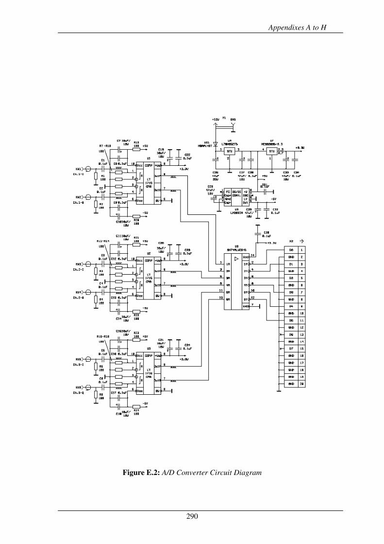
Appendixes A to H
290
Figure E.2: A/D Converter Circuit Diagram

Appendixes A to H
291
E.2 Sampling Clock
Table E-2: Sampling clock module part list
Position Part number Value Case Qty Producer
C2, C4-C9 06033G104ZAT2A 0.1 uF Y5V 25V 603 7 AVX
C3 TPSA106K010R1800 10uF-10V A 9 AVX
C1 TAJD476K025R 47uF-25V D 1 AVX
U1 HCD311/BNDN OCXO 1 Golledge
U2 L78M05CTD 5V Voltage regulator DPAK 1 STM
U3 74AC04PC Hex inverter DIP-14 1 Fairchild
U4 74AC191PC 4-bit counter SOIC-16 1 Fairchild
R1-4 MC 0.063W 0603 5% 100R 100 Ohm 603 4 Multicomp
VD1 MBRA140T 1A-40V Shottky SMA 1
International
Rectifier
X1 SMT 2.5MM POWER SOCKET 1
X2
20 WAY STRAIGHT BOX
HEADERS FCI RC 1
XW1, 2
SMA 50 Ohm PCB end launch
connector 19-70-TGG 2 MULTICOMP
F1, 2 PLP-10.7 10,7MHz LPF 2 Minicircuits
Table E2 above gives the details of all parts for the sampling clock module. The 50
MHz sampling clock is generated by the OCXO, and see its specification are given in
the data sheet below.

Appendixes A to H
292
E.3 Data Acquisition Card
• 1 bit to 16 bit digital I/O
• Special 1, 2 and 4 bit digital I/O mode (Mi.7005 only).
• 3,3 V and 5 V compatible TTL I/O
• 1 ks/s up to 125 Ms/s sample rate
• Up to 512 Mbyte memory
• Enhanced trigger possibilities
• Replay and record possible at the same time
Figure E.3: Data acquisition card and docking station
Options included
• FIFO mode
• External TTL trigger input/output
• External TTL clock input/output
• Pattern and edge trigger
• Pulse width trigger
• Basic memory: 16 Mbyte
• 1 to 4 bit memory efficient mode
• Input impedance selectable to 110 Ohm or 1 MOhm

Appendixes A to H
293
The digital data acquisition card offers a resolution between 1 bit and 16 bits with a
maximum sample rate of 125 Msamples/s. Each of the 16 1-bit resolution channels of
the board can be separately programmed for input or output. The entire on-board
memory of up to 16 Mbytes can be used for recording or replaying digital data or the
board can be used in a FIFO mode, which is designed for continuous data transfer
between a measurement board and the PC memory (up to 100 Mbytes/s) or hard disk
(up to 50 Mbytes/s). The data stream is controlled automatically by the interrupt
request on the driver. A sampling clock can be supplied from an external system
using an external connector and it is possible to output the internally used sampling
clock to synchronize external equipment. The internal standard synchronization bus
allows synchronization of several boards.
E.4 Software for Data Acquisition
The customized data acquisition software applies the FIFO mode of the data
acquisition card to record the data continuously, and transfer it to the hard disk
directly. The on-board memory is used as a continuous buffer and the data must be
read from the board with at least as high a speed as the speed of data collected in. If
the data is read from the board more slowly, the hardware buffers will overrun and the
FIFO mode will be stopped.
Figure E.3 shows the working schema of the FIFO mode. On the hardware side, the
board memory is split into two buffers of the same length. These buffers can be up to
half of the on-board memory in size. In addition to the hardware buffers, the software
driver holds up to 256 software buffers of the same length as the hardware buffers (at

Appendixes A to H
294
present 64 software buffers can satisfy the experiment usage, as confirmed by testing).
Whenever a hardware buffer is full with data the hardware generates an interrupt and
the software driver transfers the contents of this hardware buffer to the next software
buffer that is available. While transferring the content of one hardware buffer to the
PC, the other is filled as an automatic background process. After processing the data,
the application software tells the driver that it can use the software buffer for data
collection again. This two-stage buffering has a big advantages when running the
FIFO at the speed limit.
Read
Buf 0
Record Buf 1
Record Buf 0Record Buf 0 Record Buf 0
Record Buf 1
Record Buf 0
Record Buf 1
Read
Buf 0
Read
Buf 1
Read
Buf 0
Read
Buf 1
Read
Buf 1
SW Buf
0
SW Buf
63
SW Buf
3
SW Buf
2
SW Buf
1
SW Buf
0
Application Software: Data recorder: Processing the 64 Software Buffers
Trigger
Interrupt InterruptInterrupt InterruptInterruptInterruptInterruptInterrupt
Hardware
Software
Figure E.4: Read Scheme of FIFO Mode
The software buffers greatly expand the acquisition time that can be buffered and
protects the whole system against buffer overrun. However, one bottleneck with the
FIFO mode is the PCI bus of host PC. The standard PCI bus is theoretically capable
of transferring 32-bit long data at the frequency of 33 MHz, so that a maximum burst
transfer of 132 Mbytes per second can be achieved. As several devices can share the
PCI bus this maximum transfer rate is only available for a short transfer burst time

Appendixes A to H
295
until new bus arbitration is necessary. In fact the continuous transfer rate is limited to
approximately 100-110 Mbytes per second. The maximum FIFO speed one can
achieve depends heavily on the PC system and the operating system and varies from
system to system. The maximum sample rate supported by the data acquisition board
depends on the working mode and the number of activated channels.
For the experimentation reported, 4-bit and 8-bit modes are used, these modes
respectively allowing maximum sample rates of 125 MSamples/s (62.5 Mbytes/s) and
100 MSamples/s (100 Mbytes/s). Abundant tests indicated that best results were
obtained when programming the buffer length to be a number of samples that can
hold approximately 100 ms of data. Here we use 64 software buffers, the size of each
being 16 kbytes. However, when operating near the speed limit of the PCI bus in the
FIFO mode or when buffer overruns, it can be useful to have larger FIFO buffers.
When the goal is a fast update in FIFO mode, smaller buffers and a larger number of
buffers can offer better performance.

Appendixes A to H
296
MI7005 Configuration
Next Half Buffer Ready?
Initial PCI Board
Software Reset
Start the Board
FIFO Mode Setup
Handling the Data
Stop
Release the Board
No
Yes
Yes
No
Figure E.5: Data Acquisition Software Flowchart
Figure E4 above shows the software flowchart of the customized data acquisition
application, which employs the data acquisition board to record the data. First, the
data acquisition board is initialized to get the board number and board type. Then the
board configuration routine defines the working mode and allocates buffer memory,
and the FIFO routine defines the clock source, the sampling rate, the trigger source
and the input impedance etc. The software “start” command and “wait” command
both wait for the signal that the next buffer has to be processed, this signal being
generated by the software driver on receiving an interrupt from the board. The
application counts all the software buffers that have been transferred and this number

Appendixes A to H
297
can be read out from the driver to know the exact amount of data that has been
transferred. Finally, after handling the data, the memory is cleared and the board
released.
The file format of the data files generated by this process is described here. The
whole of a file is a data block, and the data is written to the file in 16-bit binary format,
with the lower byte first (little endian). For example, the value 0x1234 is written to
disk with 34 first followed by 12. The total length of the data block depends on the
data width and the total data count. Because the file is written in binary format, any
binary file editor can be used to view it or functions designed for reading files can be
used to get the file information and data values.
The software mentioned above stores the data as a single sequence, so it is necessary
to extract the data supplied by the different channels from this sequence. By
performing bit manipulation, each stored byte is extracted and divided into four or
eight parts, each bit pair (associated with a particular channel) being saved
individually. After this process, the raw data will have been split into four or eight
files with identical size, each relevant to a different channel.
E.5 Data Acquisition Subsystem Testing
The data acquisition subsystem test consisted of testing the ADC board and the data
acquisition card separately at the beginning; the assembled subsystem was then tested
with a sine wave and a square wave as inputs, the stored data was used to reconstruct
the input signal with MATLAB, allowing checks of the working frequency range and

Appendixes A to H
298
the lowest permissible input amplitude of subsystem. Transmission line effects and
environment noise, particularly on clock and control lines, also require attention. It is
advisable to use twisted-pair connections to the data acquisition card, each digital I/O
signal line being twisted with a GND line, and to place a shield around the wires.
Figure E6 below shows the testing setup for the whole data acquisition subsystem.
With a baseband 10 MHz PRN sequence generated by AMIQ generator, this analogue
input signal has been converted to digital bits, sampled by data acquisition card with
50 MHz clock, and written into files on the hard disk.
Figure E.6: Experimental Set-up for DAQ Testing
Figure E.7:Photo of Experimental Set-up

Appendixes A to H
299
The stored data has then been divided into multiple files for each channel and the
correlation with locally generated PRN code has been used for a data integrity check.
Figure E8 below show the correlation results. Figure E.8 (a) shows the mainlobe of
the correlation peak between the stored data from one channel and the reference code;
and Figure E.8 (b) shows the zoomed version. It can be clearly seen that the width of
mainlobe is 0.1 us which corresponds to 10 MHz symbol rate. Figures E.8(c) and
E.8(d) plot the sidelobe level of the correlation peak in both decimal and log scales. It
reaches the expected theoretical value of -90 dB (as the PRN code is generated from
15 bit shift feedback registers). From these results the full function of data acquisition
subsystem has been confirmed and it’s ready for the further testing with the
microwave receiver.
0 0.2 0.4 0.6 0.8 1 1.2 1.4-100
-90
-80
-70
-60
-50
-40
-30
-20
-10
0
Delay (us)
Co
rre
latio
n m
ag
nitu
de
(d
B)
ACF 15 bit M-seq DAQ
(a) correlation peak main lobe
0.02 0.04 0.06 0.08 0.1 0.12 0.14 0.16 0.18 0.2
-90
-80
-70
-60
-50
-40
-30
-20
-10
Delay (us)
Co
rre
latio
n m
ag
nitu
de
(d
B)
ACF 15 bit M-seq in L
(b) zoom of (a)

Appendixes A to H
300
0 10 20 30 40 50 60-90.5
-90
-89.5
-89
-88.5
-88
-87.5
-87
-86.5
-86
Integration Time (s)
Sid
elo
be
Le
ve
l (d
B)
(c) correlation sidelobe level
10-3
10-2
10-1
100
101
102
-90.4
-90.2
-90
-89.8
-89.6
-89.4
-89.2
-89
-88.8
-88.6
-88.4
Integration Time (s)
Sid
elo
be
Le
ve
l (d
B)
(d) log scale of (c)
Figure E.8: Data Acquisition Subsystem Testing Results

Appendixes A to H
301
Appendix F GPS Receiver
The Legacy-E (Topcon) GNSS receiver is used in the radar. It based on a full
function Euro Card design, which allows use of GPS and/or GLONASS L1 and
L1/L2. The Legacy-E features dual frequency ability with GPS, or single with
GPS+GLONASS signals. Based around a half Euro Card, it is one of the smallest
high performance GPS units available on the market. A photo of the Legacy-E
receiver and its antenna are shown below.
Brief specification:
• 1 x Legacy E GGD GPS+ Base Station
• 40 Super Channel Receiver
• L1+L2 GPS/GLONASS
• Advanced Multipath Reduction
• 96Mb Data Recording
• Base Case
• 7ah Battery / Charger
• PGA-1 GPS Antenna with cable
• Co-op Tracking (low elevation, under canopy)
• Base Case Complete
• Heavy Duty Wooden Tripod
• PC-CDU Lite Interface Software

Appendixes A to H
302
Appendix G Microwave Receiver – Testing Results
As discussed in Chapter 5, more details are given in this section for the hardware
design and testing of the microwave receiver. Table G1 below lists the information
for all microwave receiver components. Most of parts are off-the-shelf commercial
products except the RF front end which is a customized designed and its specification
included in Appendix C. In this Appendix, specifications for all other parts will be
given and testing results for different blocks and the full microwave receiver will be
presented and discussed.
A series of testing stages in the laboratory has been performed according the
following categories:
1. Power supply test, DC and AC coupling
2. Local oscillator test, frequency synthesizer
3. IF and baseband blocks test, IF gain and quadrature demodulator distortion
4. Full receiver test with noise and input signal

Appendixes A to H
303
Table G-1: Microwave Receiver Parts List
The process for these testing categories has been described briefly and the main
results are noted below.
• Power Supply Test, DC and AC coupling
Given different input voltages applied to the DC-DC converter, the working range and
the converter output voltage are established. From these results, the DC-DC
converters work consistently and accurately over a wide range of input voltages.
Using an AD-3521 FFT analyzer, it tests the AC coupling at the external power
supply, the output of the DC-DC converter and the capacitor board to check the
external interference and environment noise applied to the microwave receiver caused
Component Specifications Model Number Supplier
RF LNA1 See Appendix C
IF Amplifiers
A1—A4
Fl –Fu: 0.05-500 MHZ,
Gain: 20 dB, NF: 5.3 dB
ZFL-500 Mini-circuits
Splitters S1 3-way 00, 1.0 -- 2.0 GHZ ZA3PD-2 Mini-circuits
Mixers M1 LO/RF: 1-4.2 GHZ ZX05-C42 Mini-circuits
IF Filter
BPF3
Fc: 140 MHz,
1 dB BW: 55.8 MHz,
Insertion Loss: < 1 dB
KR 2743
KR
Electronics
Splitters S2 3-way 00, 1 -- 500 MHz ZFSC-3-1 Mini-circuits
Splitters S3 2-way 00, 2 -- 1200 MHz ZX10-2-12 Mini-circuits
Splitters S4 2-way 900, 120 - 180 MHz
ZMSCQ-2-180 Mini-circuits
Mixers M2 LO/RF: 0.5-500 MHZ,
IF: DC-500 MHz
ZLW-1H Mini-circuits
Amplifier A5 Fl –Fu: 0.01-1GHz ZFL-1000VH Mini-circuits
LPF1 Pass Band: DC-32 MHZ SLP-30 Mini-Circuits

Appendixes A to H
304
by these components. Table G-2 below shows the AC coupling testing results.
Although this interference extends into the working frequency range of the microwave
receiver, the extremely low amplitude implies little effect upon the wanted signal.
Table G-2: AC Coupling Test Results
Power Supply Unit Frequencies Level
50 Hz -68 dBV to –80 dBV External Power Supply
Input: 220 V AC, Output: 12 V
DC
66.4 kHz -43 dBV
50 Hz -80 to -102 dBV
25 kHz -107 dBV or less
Internal DC-DC Converter
Input: 12 V DC Output: 15 V DC
424 kHz -36 dBm to –67 dBm
At capacitor board 15 V 424 kHz -49 dBm to –70 dBm
Internal DC-DC Converter
Input: 12 V DC Output: 5 V DC
410 kHz -44 dBm
• Local oscillator test, frequency synthesizer
During the experiments using GLONASS, two synchronized Rohde & Schwarz signal
generators are locked with a common clock and used as a local oscillator. During the
experiments using Galileo, as the compact hardware is required for field trials, two
frequency synthesizers have been used to replace the signal generators. The test
procedure is to find the appropriate output level of the local oscillator using a
spectrum analyzer, comparing with the working range of the power splitter and the
ZFL-1000VH amplifier. Table G-3 below shows the output level from each point.

Appendixes A to H
305
Table G-3: Frequency Synthesizer Test Results
Generator Frequency Output Level
Frequency synthesizer 1 1347.14 MHz 10 dBm
Frequency synthesizer 1 140 MHz 6 dBm
Power Splitters and LO 2 amplifier
Component Frequency of operation Insertion loss/Gain
Power splitter 1(ZA3PD-2) 1347.14 MHz at the input ~ 6 dB
Power splitter 2 (ZA3PD-2) 140 MHz ~ 5.5 dB
Power splitter (ZMSCQ-2-90) 140 MHz ~3 dB
Local oscillator amplifier
(ZFL-1000VH)
140 MHz ~ 22 dB
To match the working amplitude of the mixers perfectly, considering the loss of the
power splitter and the amplifier gain, the output level of LO1 and LO2 will be set as
10 dBm and 6 dBm individually.
• In-Phase/Quadrature Demodulator Distortion (Baseband Block) Test
The goal of the testing is to check the amplitude unbalance between the in-phase and
quadrature channels. See Figure G.1 below for the testing diagram. A 140 MHz sine
wave is used as a IQ demodulator input, with the combined I/Q signals vectors shown
on the screen of the two-channel oscilloscope.

Appendixes A to H
306
S p litte r
0o
S p litte r
9 0 o
L P F
L P F
I
Q
Inp u t, 1 4 0 M H z, 2d B m LO : 1 4 0 M H z
Figure G.1: I/Q Demodulator Distortion Test Diagram
Figure G.2: I/Q vectors
In the diagram (Figure G.2) shown above the vertical and horizontal scales are equal.
A nearly perfect circle is shown, indicating that the I and Q channels are balanced.
The goal of next testing phase is to check whether the microwave receiver can down-
convert the input to baseband signal successfully. A 50-ohm load was connected to
the input and the frequency response observed with a spectrum analyzer. The output
spectrum after the IF bandpass filter and the entire IF amplifier has the centre
frequency (140 MHz) and bandwidth (50 MHz), confirming the response of the IF
filter.
Heterodyne Channel Radar Channel Low-gain Channel

Appendixes A to H
307
The second step is to provide a BPSK signal as the input of the receiver and test the
channels without IF amplifiers and without a SAW filter (to avoid IF amplifier
saturation due to high gain). See Figure G.3 below for testing procedure. For the test,
the signals are displayed and stored using the oscilloscope.
RF Filter
LNA
Mixer
BPF
(mini-circuit)
Baseband
unit
I
Q
1347.14MHz
NO IF amplifiers
BPSK
signal
Figure G.3: Test Diagram
• Full receiver test with noise and input signal
Figure G.4 below shows the diagram for receiver noise testing procedure. No input
signal will be applied and a 50 ohm load was connected at the RF input of the
microwave receiver. Only the receiver noise will appear at the input of data
acquisition subsystem, sampled and stored into the host PC.
Figure G.4: Receiver Noise Test Diagram
Figures G.5 below show the correlation results. Figure G.5 (a) shows the mainlobe of
auto-correlation peak of the receiver noise in channel R; and Figure G.5 (b) shows its

Appendixes A to H
308
sidelobe level. Figures G.5 (c) and G.5(d) plot the similar results for channel H.
Figures G.5(e) and G.5(f) plot the cross-correlation of the noise between two
channels. From these results the receiver noise behaves as expected and no strong
internal interference was detected.
0 0.2 0.4 0.6 0.8 1 1.2 1.4-80
-70
-60
-50
-40
-30
-20
-10
0
Delay (us)
Co
rre
latio
n m
ag
nitu
de
(d
B)
(a) ACF of noise in R-channel
10-3
10-2
10-1
100
101
102
-68
-66
-64
-62
-60
-58
-56
Integration Time (s)
Sid
elo
be
Le
ve
l (d
B)
(b) sidelobe level of (a)
0 0.2 0.4 0.6 0.8 1 1.2 1.4-70
-60
-50
-40
-30
-20
-10
0
Delay (us)
Co
rre
latio
n m
ag
nitu
de
(d
B)
ACF noise in H
(c) ACF of noise in H-channel
10-3
10-2
10-1
100
101
-57
-56.5
-56
-55.5
-55
-54.5
-54
-53.5
Integration Time (s)
Sid
elo
be
Le
ve
l (d
B)
(d) sidelobe level of (c)
0 0.2 0.4 0.6 0.8 1 1.2 1.4-50
-45
-40
-35
-30
-25
-20
-15
-10
-5
0
Delay (us)
Co
rre
latio
n m
ag
nitu
de
(d
B)
CCF noise in H&R
(e) CCF of noise between H and R
channels
10-3
10-2
10-1
100
101
-44
-42
-40
-38
-36
-34
-32
-30
Integration Time (s)
Sid
elo
be
Le
ve
l (d
B)
(f) sidelobe level of (e)
Figure G.5: Receiver Noise Testing Results

Appendixes A to H
309
Figure G.6: Test Diagram for Receiver with Input Signal
Figure G.6 above shows the diagram for receiver input signal testing procedure. An
input signal with 1191.795 MHz frequency and 10 MHz bandwidth will be applied at
the RF input of the microwave receiver. Both the receiver noise and the signal output
will appear at the input of the data acquisition subsystem, sampled and stored into the
host PC.
Figure G.7: Photo of Satellite Imitator (Signal Generator)

Appendixes A to H
310
0 0.2 0.4 0.6 0.8 1 1.2 1.4-90
-80
-70
-60
-50
-40
-30
-20
-10
0
Delay (us)
Co
rre
latio
n m
ag
nitu
de
(d
B)
(a) ACF of L-channel signal
10-3
10-2
10-1
100
101
-78.5
-78
-77.5
-77
-76.5
-76
-75.5
Integration Time (s)
Sid
elo
be
Le
ve
l (d
B)
(b) sidelobe level of (a)
0 0.2 0.4 0.6 0.8 1 1.2 1.4-120
-100
-80
-60
-40
-20
0
Delay (us)
Co
rre
latio
n m
ag
nitu
de
(d
B)
CCF in R&L
(c) CCF between L-channel and R-
channel signals
0 0.05 0.1 0.15 0.2 0.25 0.3 0.35 0.4
-90
-80
-70
-60
-50
-40
-30
-20
-10
0
(d) zoom of (c)
0 10 20 30 40 50 60-90
-85
-80
-75
-70
-65
-60
-55
-50
-45
Integration Time (s)
Sid
elo
be
Le
ve
l (d
B)
(e) sidelobe level of (c)
10-3
10-2
10-1
100
101
102
-90
-85
-80
-75
-70
-65
-60
-55
-50
Integration Time (s)
Sid
elo
be
Le
ve
l (d
B)
(f) log scale of (e)
Figure G.8: Results for correlation between radar and low-gain channels
Figure G.8 above shows the correlation results. Figure G.8 (a) shows the mainlobe of
the auto-correlation peak of stored signal in channel L; and Figure G.8 (b) shows its
sidelobe level. Figures G.8(c) and G.8(d) plot the cross-correlation of the stored

Appendixes A to H
311
signals from the L and R channels. It can be clearly seen that the width of mainlobe is
0.1 us which corresponds to a 10 MHz bandwidth. Figures G.8(e) and G.8(f) display
the sidelobe of CCF.
0 0.2 0.4 0.6 0.8 1 1.2 1.4-100
-90
-80
-70
-60
-50
-40
-30
-20
-10
0
Delay (us)
Co
rre
latio
n m
ag
nitu
de
(d
B)
ACF M-seq in L
(a) ACF of L-channel signal
0 0.2 0.4 0.6 0.8 1 1.2 1.4-80
-70
-60
-50
-40
-30
-20
-10
0
Delay (us)
Co
rre
latio
n m
ag
nitu
de
(d
B)
ACF M-seq+noise in H
(b) ACF of H-channel signal
10-3
10-2
10-1
100
-64
-63
-62
-61
-60
-59
-58
Integration Time (s)
Sid
elo
be
Le
ve
l (d
B)
(c) log scale sidelobe level of (b)
0 0.2 0.4 0.6 0.8 1 1.2 1.4-120
-100
-80
-60
-40
-20
0
Delay (us)
Co
rre
latio
n m
ag
nitu
de
(d
B)
CCF in H&L
(d) CCF between L- and H-channels
10-3
10-2
10-1
100
101
102
-90
-85
-80
-75
-70
-65
-60
-55
-50
-45
Integration Time (s)
Sid
elo
be
Le
ve
l (d
B)
(e) log scale sidelobe level of (d)
Figure G.9: Results for correlation between heterodyne and low-gain channels

Appendixes A to H
312
Figures G9 above show the similar results to Figure G.8, the only difference is
channel L and H used this time. Figure G.9 (a) shows the mainlobe of auto-
correlation peak of stored signal in channel L; and Figure G.9 (b) and G.9(c) show
auto-correlation peak of stored signal in channel H and its sidelobe level. Figures
G.9(d) and G.9(e) plot the cross-correlation of the stored signals from L and R
channels and the sidelobe of cross correlation function.
1. Galileo Open Service Signal In Space Interface Control Document. 2006,
European Space Agency / Galileo Joint Undertaking.

Publications List
- 313 -
Appendix H Publications List
� Cherniakov, M., Antoniou, M., Saini, R., Zuo, R., & Edwards, J. (2006). Space-
Surface BSAR - Analytical and Experimental study. Paper presented at the EuSAR
conference, Dresden, Germany.
� Cherniakov, M., Saini, R., Antoniou, M., Zuo, R., & Edwards, J. (2006). Modified
Range-Doppler algorithm for Space-Surface BSAR imaging. Paper presented at the
Radar 2006, China.
� Cherniakov, M., Saini, R., Antoniou, M., Zuo, R., & Edwards, J. (2006). Signal
Processing in space-surface bistatic synthetic aperture radar. Paper presented at the
International Conference on Synthetic Aperture Sonar and Synthetic Aperture Radar,
Lerici, Italy.
� Cherniakov, M., Saini, R., Antoniou, M., Zuo, R., & Edwards, J. (2006). SS-BSAR
with Transmitter of Opportunity - Practical Aspect. Paper presented at the EMRS
DTC Conference, Edinburgh, UK.
� Zuo, R., Saini, R., & Cherniakov, M. (2007). Non-cooperative Transmitter Selections
for Space-Surface Bistatic SAR. Paper presented at the EMRC DTC 2007 conference,
Edinburgh, UK.
� Saini, R., Zuo, R., & Cherniakov, M. (2007). Signal synchronisation in SS-BSAR
based on GLONASS satellite emission. Paper presented at the Radar 2007,
International conference, Edinburgh, UK.
� Cherniakov, M., Saini, R., Zuo, R., & Antoniou, M. (2007). Space-Surface Bistatic
Synthetic Aperture Radar with GNSS transmitter of opportunity-Experimental
Results, . IET Proceedings Radar, Sonar and Navigation, 1(6), 447 - 458.
� Antoniou, M., Saini, R., Cherniakov, M., & Zuo, R. (2007). Image Formation
Algorithm for Space-Surface BSAR. Paper presented at the EuRAD 2007 conference,
Munich, Germany.
� Zuo, R., Saini, R., Antoniou, M., & Cherniakov, M. (2008). Development of a
Passive BSAR with GNSS Transmitters of Opportunity. Paper presented at the EMRC
DTC 2008 conference, Edinburgh, UK.

Publications List
- 314 -
� Saini, R., Zuo, R., & Cherniakov, M. (2008). Development of space-surface Bistatic
synthetic aperture radar with GNSS transmitter of opportunity. Paper presented at the
IEEE Radar Conference 2008, Rome, Italy.
� Cherniakov, M., Saini, R., Antoniou, M., Zuo, R., & Plakidis, E. (2008). Experiences
Gained during the Development of a Passive BSAR with GNSS Transmitters of
Opportunity. International Jounal of Navigation and Observation, 2008. doi:
10.1155/2008/807958
� Zuo, R., Antoniou, M., Plakidis, E., & Cherniakov, M. (2009). Passive bistatic
imaging using Galileo transmitters. Paper presented at the EMRC DTC 2009
conference, Edinburgh, UK.
� Saini, R., Zuo, R. (communication author), & Cherniakov, M. (2009). Problem of
Signal Synchronisation in SS-BSAR based on Global Navigation Satellite Emissions
- Experimental Results. IET Proceedings Radar, Sonar and Navigation, 4(1), 110 -
125.