Bispectral and glN glM dualities, discrete versus differential · The regularized fundamental...
50
Advances in Mathematics 218 (2008) 216–265 www.elsevier.com/locate/aim Bispectral and (gl N , gl M ) dualities, discrete versus differential E. Mukhin a , V. Tarasov a,b,1 , A. Varchenko c,∗,2 a Department of Mathematical Sciences, Indiana University – Purdue University, Indianapolis, 402 North Blackford street, Indianapolis, IN 46202-3216, USA b St. Petersburg Branch of Steklov Mathematical Institute, Fontanka 27, St. Petersburg, 191023, Russia c Department of Mathematics, University of North Carolina at Chapel Hill, Chapel Hill, NC 27599-3250, USA Received 6 December 2006; accepted 29 November 2007 Available online 28 January 2008 Communicated by Michael J. Hopkins Abstract We define integral transforms which establish a correspondence between spaces of quasi-exponentials and spaces of quasi-polynomials under certain conditions. As a corollary of the properties of our transforms we obtain a correspondence between solutions to the Bethe ansatz equations of two (gl N , gl M ) dual quan- tum integrable models: one is the special trigonometric Gaudin model and the other is the special XXX model. © 2007 Elsevier Inc. All rights reserved. Keywords: Bethe ansatz; Critical point; Integral transform 1. Introduction Let V =x λ i p ij (x), i = 1,...,n, j = 1,...,N i be a space of quasi-polynomials in x of dimension N = N 1 +···+ N n . The regularized fundamental differential operator of V is the polynomial differential operator ∑ N i =0 A N −i (x)(x∂ x ) i annihilating V and such that its leading coefficient A 0 is a monic polynomial of the minimal possible degree. * Corresponding author. E-mail address: [email protected] (A. Varchenko). 1 Supported in part by RFFI grant 05-01-00922. 2 Supported in part by NSF grant DMS-0244579. 0001-8708/$ – see front matter © 2007 Elsevier Inc. All rights reserved. doi:10.1016/j.aim.2007.11.022
Transcript of Bispectral and glN glM dualities, discrete versus differential · The regularized fundamental...

Advances in Mathematics 218 (2008) 216–265www.elsevier.com/locate/aim
Bispectral and (glN,glM) dualities, discrete versusdifferential
E. Mukhin a, V. Tarasov a,b,1, A. Varchenko c,∗,2
a Department of Mathematical Sciences, Indiana University – Purdue University, Indianapolis,402 North Blackford street, Indianapolis, IN 46202-3216, USA
b St. Petersburg Branch of Steklov Mathematical Institute, Fontanka 27, St. Petersburg, 191023, Russiac Department of Mathematics, University of North Carolina at Chapel Hill, Chapel Hill, NC 27599-3250, USA
Received 6 December 2006; accepted 29 November 2007
Available online 28 January 2008
Communicated by Michael J. Hopkins
Abstract
We define integral transforms which establish a correspondence between spaces of quasi-exponentialsand spaces of quasi-polynomials under certain conditions. As a corollary of the properties of our transformswe obtain a correspondence between solutions to the Bethe ansatz equations of two (glN,glM) dual quan-tum integrable models: one is the special trigonometric Gaudin model and the other is the special XXXmodel.© 2007 Elsevier Inc. All rights reserved.
Keywords: Bethe ansatz; Critical point; Integral transform
1. Introduction
Let V = 〈xλi pij (x), i = 1, . . . , n, j = 1, . . . ,Ni〉 be a space of quasi-polynomials in x ofdimension N = N1 + · · · + Nn. The regularized fundamental differential operator of V is thepolynomial differential operator
∑Ni=0 AN−i (x)(x∂x)
i annihilating V and such that its leadingcoefficient A0 is a monic polynomial of the minimal possible degree.
* Corresponding author.E-mail address: [email protected] (A. Varchenko).
1 Supported in part by RFFI grant 05-01-00922.2 Supported in part by NSF grant DMS-0244579.
0001-8708/$ – see front matter © 2007 Elsevier Inc. All rights reserved.doi:10.1016/j.aim.2007.11.022

E. Mukhin et al. / Advances in Mathematics 218 (2008) 216–265 217
Let U = 〈zuaqab(u), a = 1, . . . ,m, b = 1, . . . ,Ma〉 be a space of quasi-exponentials in u
of dimension M = M1 + · · · + Mm. The regularized fundamental difference operator of U isthe polynomial difference operator
∑Mi=0 BM−i (u)(τu)
i annihilating U and such that its leadingcoefficient B0 is a monic polynomial of the minimal possible degree. Here (τuf )(u) = f (u+ 1).
We introduce the notion of a nondegenerate space of quasi-polynomials in Section 2 and thenotion of a nondegenerate space of quasi-exponentials in Section 3.
Having a nondegenerate space V of quasi-polynomials with the regularized fundamen-tal differential operator
∑Ni=0 AN−i (x)(x∂x)
i , we construct a nondegenerate space of quasi-exponentials U = 〈zu
aqab(u)〉 whose regularized fundamental difference operator is the differ-ence operator
∑Ni=0 uiAN−i (τu). The space U is constructed from V by a suitable integral
transform.Having a nondegenerate space U = 〈zu
aqab(u)〉 of quasi-exponentials with the regularizedfundamental difference operator
∑Mi=0 BM−i (u)(τu)
i , we construct a nondegenerate space ofquasi-polynomials V = 〈xλi pij (x)〉 whose regularized fundamental differential operator is thedifferential operator
∑Mi=0 xiBM−i (x∂x). The space V is constructed from U by a suitable inte-
gral transform.Our integral transforms are analogs of the bispectral involution on the space of rational solu-
tions to the KP hierarchy [24].As a corollary of the properties of our integral transforms we obtain a correspondence between
solutions to the Bethe ansatz equations of two (glN,glM) dual quantum integrable models: oneis the special trigonometric Gaudin model and the other is the special XXX model.
Example. Let n = (n1, n2) and m = (m1,m2) be two vectors of nonnegative integers suchthat n1 + n2 = m1 + m2. Let d be the number of integers i such that max(0, n2 − m1) � i �min(m2, n2). Let z = (z1, z2),λ = (λ1, λ2) ∈ C2 be two points with distinct coordinates.
Consider two systems of algebraic equations. The first system is the system of equations
λ1 − λ2 − 1
ti+
2∑a=1
ma
ti − za
−n2∑
j=1,j �=i
2
ti − tj= 0, i = 1, . . . , n2, (1.1)
with respect to the unknown numbers t1, . . . , tn2 . The system is symmetric with respect to thegroup Σn2 of permutations of t1, . . . , tn2 . One can show that for generic z,λ the number of Σn2 -orbits of solutions of system (1.1) is equal to d . This system is called the system of the GaudinBethe ansatz equations, see Section 10.5.
The second systems of equations is the system
2∏i=1
sa − λi − 1
sa − λi − 1 − ni
m2∏b,b �=a
sa − sb − 1
sb − sb + 1= z2
z1, a = 1, . . . ,m2, (1.2)
with respect to the unknown numbers s1, . . . , sm2 . The system is symmetric with respect to thegroup Σm2 of permutations of s1, . . . , sm2 . One can show that for generic z,λ the number ofΣm2 -orbits of solutions of system (1.2) with distinct s1, . . . , sm2 is equal to d . This system iscalled the system of the XXX Bethe ansatz equations, see Section 10.5.
Problem. Establish a correspondence between orbits of solutions to systems (1.1) and (1.2).

218 E. Mukhin et al. / Advances in Mathematics 218 (2008) 216–265
We give two solutions to this problem.
The first solution. To system (1.1), we assign the vector space (Lm1 ⊗ Lm2)[n1, n2] and fourcommuting linear operators acting on this space. Here (Lm1 ⊗ Lm2)[n1, n2] denotes the weightsubspace of weight [n1, n2] of the tensor product of irreducible gl2-modules with highest weights(m1,0) and (m2,0), respectively. The space (Lm1 ⊗ Lm2)[n1, n2] is of dimension d . The linearoperators are denoted by
HG1 (λ1 + n1, λ2 + n2,z), HG
2 (λ1 + n1, λ2 + n2,z),
GG1 (λ1 + n1, λ2 + n2,z), GG
2 (λ1 + n1, λ2 + n2,z)
and called the Gaudin KZ and dynamical Hamiltonians. To each orbit of solutions of system(1.1), the Bethe ansatz method assigns an eigenvector of the commuting Hamiltonians. The con-structed Bethe vectors form a basis of this vector space.
To system (1.2), we assign the vector space (Ln1 ⊗ Ln2)[m1,m2] of the same dimension d
and four commuting linear operators acting on this space. The linear operators are denoted by
HX1 (z, λ1 + n1, λ2 + n2), HX
2 (z, λ1 + n1, λ2 + n2),
GX1 (z, λ1 + n1, λ2 + n2), GX
2 (z, λ1 + n1, λ2 + n2)
and called the XXX KZ and dynamical Hamiltonians. To each orbit of solutions of system (1.2),the Bethe ansatz method assigns an eigenvector of the commuting Hamiltonians. The constructedBethe vectors form a basis of this vector space.
There is a natural isomorphism of the vector spaces (Lm1 ⊗ Lm2)[n1, n2] and(Ln1 ⊗ Ln2)[m1,m2], which identifies the Hamiltonians:
HGa (λ1 + n1, λ2 + n2,z) = GX
a (z, λ1 + n1, λ2 + n2),
GGi (λ1 + n1, λ2 + n2,z) = HX
i (z, λ1 + n1, λ2 + n2),
for i, a = 1,2. This isomorphism is called the (gl2,gl2)-duality, see [22]. Under the duality iso-morphism the Bethe vectors are identified and this identification gives a correspondence betweenthe orbits of solutions of systems (1.1) and (1.2).
The second solution. To the orbit of a solution (t1, . . . , tn2) of system (1.1), we assign the poly-nomial p2(x) = ∏n2
i=1(x − ti ) and the differential operator
D = x2(x − z1)(x − z2)
(∂x − ln′
(xλ1−1 ∏2
a=1(x − za)ma
p2
))(∂x − ln′(xλ2p2
)),
where ∂x = d/dx and for any function f , ln′ f denotes the logarithmic derivative f ′/f . Clearlythe differential equation Df (x) = 0 has a solution xλ2p2(x).
We show that D can be written in the form
D = A0(x)(x∂x)2 + A1(x)x∂x + A2(x)
E. Mukhin et al. / Advances in Mathematics 218 (2008) 216–265 219
where A0,A1,A2 are polynomials in x of degree not greater than two. Then we consider thesecond-order difference equation(
u2A0(τu) + uA1(τu) + A2(τu))g(u) = 0
for the unknown function g(u). It turns out that this difference equation has a solution of the formzu
2q2(u), where q2(u) = ∏m2a=1(u− sa), and the roots s1, . . . , sm2 form a solution of system (1.2).
This construction gives a second correspondence between the orbits of solutions of systems (1.1)and (1.2).
We show that the two described constructions (the first, based on the (gl2,gl2)-duality, andthe second, which uses the differential and difference operators) give the same correspondencebetween solutions of systems (1.1) and (1.2).
This paper is a development of results of the paper [10], in which we presented an integraltransform giving an involution on the space of quasi-exponentials, the involution which corre-sponds to the bispectral involution of G. Wilson in [24].
The paper has the following structure. In Section 2, we discuss spaces of quasi-polynomialsand their fundamental differential operators. In Section 3, we discuss spaces of quasi-exponentialsand their fundamental difference operators. In Section 4, we define integral transforms establish-ing a duality between spaces of quasi-polynomials and quasi-exponentials. In Section 5, weintroduce rigged spaces of quasi-polynomials and quasi-exponentials. We introduce rigged in-tegral transforms relating the rigged spaces. In Section 6, we discuss relations between riggedspaces and solutions of the Bethe ansatz equations. The rigged spaces of quasi-polynomials cor-respond to solutions of the Bethe ansatz equations in the (trigonometric) Gaudin model. Therigged spaces of quasi-exponentials correspond to solutions of the Bethe ansatz equations in theXXX model. The number of solutions of the Bethe ansatz equations is discussed in Section 7.We describe the Gaudin and XXX models in Section 8. The (glN,glM) duality between the(trigonometric) Gaudin and XXX models is defined in Section 9. In Section 9, we formulate aconjecture about the bispectral correspondence of Bethe vectors under the (glN,glM) duality. InSection 10, we prove the conjecture for N = M = 2. In Section 11, we discuss the relation of ourintegral transforms with the bispectral correspondence of suitable Baker–Akhiezer functions fordifferential and difference operators.
2. Spaces of quasi-polynomials
2.1. Definition
Let p ∈ C[x] be a polynomial, λ a complex number. The function xλp(x) is called a quasi-polynomial in x. The quasi-polynomial is a multi-valued function. Different local univaluedbranches of the function differ by a nonzero constant factor.
Let N1, . . . ,Nn be natural numbers. Set N = N1 + · · · + Nn. For i = 1, . . . , n, let 0 < ni1 <
· · · < niNibe a sequence of positive integers. For i = 1, . . . , n, j = 1, . . . ,Ni , let pij ∈ C[x] be a
polynomial of degree nij .Let λ1, . . . , λn ∈ C be distinct numbers such that λi − λj /∈ Z for i �= j .Denote by V the complex vector space spanned by functions xλi pij (x), i = 1, . . . , n,
j = 1, . . . ,Ni . The dimension of V is N .The space V is called the space of quasi-polynomials.We say that the space V is nondegenerate if for any i = 1, . . . , n, and any j = 1, . . . ,Ni ,

220 E. Mukhin et al. / Advances in Mathematics 218 (2008) 216–265
• there exists a linear combination of polynomials pi1,pi2, . . . , piNiwhich has a root of mul-
tiplicity j − 1 at x = 0,• the space V does not contain the function xλi+nij .
2.2. Exponents
Let V be the space of quasi-polynomials.For z ∈ C∗, define the sequence of exponents of V at z as the unique sequence of integers,
e = {e1 < · · · < eN }, with the property: for i = 1, . . . ,N , there exists f ∈ V such that f has aroot at x = z of multiplicity ei .
We say that z ∈ C∗ is a singular point of V if the set of exponents of V at z differs from theset {0, . . . ,N − 1}. The space V has at most finitely many singular points.
Let (z1, . . . , zm) be the subset of C∗ of all singular points of V . For a = 1, . . . ,m, let
{0 < · · · < N − Ma − 1 < N − Ma + ma1 < · · · < N − Ma + maMa }be the exponents of V at za . Here 0 < ma1 < · · · < maMa and Ma is an integer such that1 � Ma � N . Set M = M1 + · · · + Mm.
We say that V is a space of quasi-polynomials with data
DV = {n,Ni, nij , λi,m,Ma,mab, za}where i = 1, . . . , n, j = 1, . . . ,Ni , a = 1, . . . ,m, b = 1, . . . ,Ma .
2.3. Fundamental differential operator
For functions f1, . . . , fi of one variable, denote by Wr(f1, . . . , fi) their Wronskian, that is,the determinant of the i × i-matrix whose j th row is fj , f
(1)j , . . . , f
(i−1)j .
Define the Wronskian of V , denoted by WrV , as the Wronskian of a basis of V . The Wron-skian of V is determined up to multiplication by a nonzero number.
Lemma 2.1. Let V be a nondegenerate space of quasi-polynomials, then
m∑a=1
Ma∑b=1
(mab + 1 − b) =n∑
i=1
Ni∑j=1
(nij + 1 − j).
The lemma is proved by analyzing the order of zeroes of the Wronskian of V and its asymp-totics at infinity.
The monic fundamental differential operator of V is the unique monic linear differential op-erator of order N annihilating V . It is denoted by DV . We have
DV = ∂Nx + A1∂
N−1x + · · · + AN , Ai = (−1)i
WrV,i
WrV,
where ∂x = d/dx, WrV is the Wronskian of a basis {f1, . . . , fN } of V , WrV,i is the determinantof the N × N -matrix whose j th row is fj , f
(1)j , . . . , f
(N−i−1)j , f
(N−i+1)j , . . . , f
(N)j .
For any j = 1, . . . ,N , the order of the pole of Aj at x = za , a = 1, . . . ,m, does not exceed j .
E. Mukhin et al. / Advances in Mathematics 218 (2008) 216–265 221
Lemma 2.2. Let V be a nondegenerate space of quasi-polynomials, then for a = 1, . . . ,m, theorder of the pole of AMa at x = za is Ma and the order of the pole of Ai is not greater than Ma
for i > Ma .
The proof follows from counting orders of determinants WV,i .The polynomial differential operator
DV = xN
m∏a=1
(x − za)Ma DV
is called the regularized fundamental differential operator of V .It is easy to see that the regularized fundamental differential operator DV of V has the form
A0(x)xN∂Nx + A1(x)xN−1∂N−1
x +· · ·+ AN(x) where Ai(x) are polynomials. Using the formulaxi∂i
x = x∂x(x∂x − 1) · · · (x∂x − i + 1) we can present the regularized fundamental differentialoperator in the form
DV = A0(x)(x∂x)N + A1(x)(x∂x)
N−1 + A2(x)(x∂x)N−2 + · · · + AN(x)
with polynomial coefficients Ai(x), i = 0, . . . ,N .
Lemma 2.3. Let V be a nondegenerate space of quasi-polynomials, then
• We have A0(x) = ∏ma=1(x − za)
Ma .
• The coefficients A0(x), . . . ,AN(x) are polynomials in x of degree not greater than M . Thesepolynomials have no common factor of positive degree.
• Write DV = xMB0(x∂x) + xM−1B1(x∂x) + · · · + xBM−1(x∂x) + BM(x∂x) whereB0(x∂x), . . . ,BM(x∂x) are polynomials in x∂x with constant coefficients. Then
B0(x∂x) =n∏
i=1
Ni∏j=1
(x∂x − λi − nij ), BM(x∂x) =m∏
a=1
(−za)Ma
n∏i=1
Ni∏j=1
(x∂x − λi − j + 1).
• The polynomials B0, . . . ,BM have no common factor of positive degree.
The proof is straightforward.
2.4. Conjugate space
Let V be a space of quasi-polynomials as in Section 2.1.The complex vector space spanned by all functions of the form Wr(f1, . . . , fN−1)/WrV with
fi ∈ V has dimension N . It is denoted by V � and called conjugate to V .The complex vector space spanned by all functions of the form f (x)x−N
∏ma=1(x − za)
−Ma
with f ∈ V � is denoted by V † and called regularized conjugate to V .

222 E. Mukhin et al. / Advances in Mathematics 218 (2008) 216–265
Lemma 2.4. Let V be a nondegenerate space of quasi-polynomials, then
(i) For a = 1, . . . ,m, if e are exponents of V at za , then
e� = {−eN − 1 + N < −eN−1 − 1 + N < · · · < −e1 − 1 + N}
are exponents of V � at za and
e† = {−eN − 1 + N − Ma < −eN−1 − 1 + N − Ma < · · · < −e1 − 1 + N − Ma}
are exponents of V † at za .(ii) For any i = 1, . . . , n, j = 1, . . . ,Ni , there exists f ∈ V † such that the function xλi+j f has
a nonzero limit as x → 0.(iii) For any i = 1, . . . , n, j = 1, . . . ,Ni , there exists f ∈ V † such that the function xλi+nij +1−Nif
has a nonzero limit as x → ∞.
The proof is straightforward.Let D = ∑
i Ai(x)∂ix be a differential operator with meromorphic coefficients. The operator
D∗ = ∑i (−∂x)
iAi(x) is called formal conjugate to D.
Lemma 2.5. Let V be a nondegenerate space of quasi-polynomials. Let DV and DV be the monicand regularized fundamental differential operators of V , respectively. Then (DV )∗ annihilatesV � and (DV )∗ annihilates V †.
The proof is straightforward.
3. Spaces of quasi-exponentials
3.1. Definition
Define the operator τu acting on functions of u as (τuf )(u) = f (u + 1).Let z be a nonzero complex number with fixed argument. Set zu = eu ln z. We have τuz
u = zuz.Let q ∈ C[u] be a polynomial. The function zuq(u) is called a quasi-exponential in u.Let M1, . . . ,Mm be natural numbers. Set M = M1 + · · · + Mm. For a = 1, . . . ,m, let 0 <
ma1 < · · · < maMa be a sequence of positive integers. For a = 1, . . . ,m, b = 1, . . . ,Ma , letqab ∈ C[u] be a polynomial of degree mab .
Let z1, . . . , zm be distinct nonzero complex numbers with fixed arguments.Denote by U the complex vector space spanned by functions zu
aqab(u), a = 1, . . . ,m,b = 1, . . . ,Ma . The dimension of U is M .
The space U is called the space of quasi-exponentials.For functions f1, . . . , fi of u, denote by Wr(d)(f1, . . . , fi) their discrete Wronskian which is
the determinant of the i × i-matrix whose j th row is fj (u), fj (u + 1), . . . , fj (u + i − 1).
Define the discrete Wronskian of U , denoted by Wr(d)U , as the discrete Wronskian of a basis
of U . The discrete Wronskian of U is determined up to multiplication by a nonzero constant.

E. Mukhin et al. / Advances in Mathematics 218 (2008) 216–265 223
Lemma 3.1. We have
Wr(d)U (u) = S(u)
m∏a=1
zMaua ,
where S(u) is a polynomial of degree∑m
a=1∑Ma
b=1(mab + 1 − b).
The proof is straightforward.
3.2. The frame of a space of quasi-exponentials
Let U be a space of quasi-exponentials like in Section 3.1. Let v1, . . . , vM be the quasi-exponentials generating U .
For i = 1, . . . ,M , let Si ∈ C[u] be the monic polynomial of the greatest degree such that thefunction Wr(d)(vj1 , vj2, . . . , vji
)/Si is regular for any j1, j2, . . . , ji ∈ {1, . . . ,M}.In particular, for the discrete Wronskian of U we have
Wr(d)U (u) = constSM(u)
m∏a=1
zMaua
with a nonzero constant.
Lemma 3.2. There exists a unique sequence of monic polynomials P1(u), . . . ,PM(u) such that
Si(u) =i∏
k=1
i−k+1∏j=1
Pk(u + j − 1)
for i = 1, . . . ,M .
This lemma is an analog of Lemma 4.12 in [14].The monic polynomials P1(u), . . . ,PM(u) are called the frame of U .
Proof. We construct Pi by induction on i. For i = 1, we set P1 = S1. Suppose the lemma isproved for all i = 1, . . . , i0 − 1. Then we set
R(u) =i0−1∏i=1
i0−i+1∏j=1
Pi(u + j − 1), Pi0(u) = Si0(u)/R(u).
We have to show that Pi0 is a polynomial. In other words, we have to show that the discreteWronskian of any i0-dimensional subspace 〈vj1, . . . , vji0
〉 is divisible by R(u).Consider the Grassmannian Gr(i0 − 2,U) of (i0 − 2)-dimensional spaces in U . For any
z ∈ C the set of points in Gr(i0 − 2,U) such that the corresponding discrete Wronskian di-vided by Si0−2 does not vanish at z, is an open set. Therefore, we have an open set of points inGr(i0 − 2,U) such that the corresponding discrete Wronskian divided by Si0−2 does not vanishat roots of R(u − 1). We call such subspaces acceptable.

224 E. Mukhin et al. / Advances in Mathematics 218 (2008) 216–265
Therefore, we have an open set of points in Gr(i0,U) such that the corresponding i0-dimensional space contains an acceptable i0 − 2 dimensional subspace. Let w1, . . . ,wi0 ∈ U besuch that w1, . . . ,wi0−2 span an acceptable space. It is enough to show that Wr(d)(w1, . . . ,wi0)
is divisible by R(u).Using discrete Wronskian identities of [14], we have for suitable holomorphic func-
tions f1, f2, g:
Wr(d)(w1, . . . ,wi0) = Wr(d)(Wr(d)(w1, . . . ,wi0−1),Wr(d)(w1, . . . ,wi0−2,wi0))
Wr(d)(w1, . . . ,wi0−2)(u + 1)
= Wr(d)(Si0−1f1, Si0−1f2)
Si0−2(u + 1)g(u + 1)= Si0−1(u)Si0−1(u + 1)
Si0−2(u + 1)
Wr(d)(f1, f2)
g(u + 1)
= R(u)Wr(d)(f1, f2)
g(u + 1).
Since the space spanned by w1, . . . ,wi0−2 ∈ U is acceptable, the functions g(u + 1) =Wr(d)(w1, . . . ,wi0−2)(u + 1)/Si0−2(u + 1) and R(u) do not have common zeros. Therefore,the discrete Wronskian Wr(d)(w1, . . . ,wi0) is divisible by R(u). �3.3. Discrete exponents
For λ ∈ C, there exists an increasing sequence of nonnegative integers {c1 < · · · < cM} and abasis {f1, . . . , fM} of U such that for i = 1, . . . ,M , we have fi(λ + j) = 0 for j = 0, . . . , ci − 1and fi(λ+ ci) �= 0. This sequence of integers is defined uniquely and will be called the sequenceof discrete exponents of U at λ. We say that the basis {f1, . . . , fM} agrees with exponents at λ.
We say that λ is a singular point of U if the discrete exponents at λ differ from the sequence{0 < 1 < · · · < M − 1}.
For i = 1, . . . ,M , introduce the local frame-type polynomials
Qi =ci−i∏
j=ci−1−i+2
(u − λ − j)
where c0 = −1. Notice that
• roots of each Qi are simple,• degQi = ci − ci−1 − 1,• sets of roots of different polynomials do not intersect,• the union of roots of all Qi is the sequence λ,λ + 1, . . . , λ + cM − M .
Theorem 3.3. Let c1 < · · · < cM be the discrete exponents of U at λ. Then
(i) The discrete Wronskian of U is divisible by
M∏ cs−M∏(u − λ − j) =
M∏M−i+1∏Qi(u + j − 1).
s=1 j=s−M i=1 j=1

E. Mukhin et al. / Advances in Mathematics 218 (2008) 216–265 225
In particular, the total degree of this divisor is∑M
i=1(ci − i + 1).(ii) If S1, . . . , SM are the polynomials from Lemma 3.2, then for any k, the polynomial Sk is
divisible by
k∏i=0
k−i+1∏j=1
Qi(u + j − 1).
Corollary 3.4. Assume that the exponents of U at λ have the form
0 < · · · < M − L − 1 < M − L + l1 < M − L + l2 < · · · < M − L + lL
for a suitable L, 1 � L � M , and 0 < l1 < · · · < lL. Then the local frame-type polynomials havethe form Qi = 1 for i = 1, . . . ,M − L,
QM−L+1 =l1−1∏j=0
(u − λ − j), QM−L+i =li−i∏
j=li−1−i+2
(u − λ − j)
for i = 2, . . . ,L, and the discrete Wronskian of U is divisible by
L∏k=1
lk−L∏j=k−L
(u − λ − j).
In particular, the total degree of this divisor is∑L
k=1(lk − k + 1).
3.4. Proof of Theorem 3.3
We shall prove part (i). Part (ii) is proved analogously.Let {f1, . . . , fM} be a basis in U that agrees with exponents at λ. Consider the matrix-valued
function F(u) = [fj (u + k − 1)]j,k=1,...,M .
Lemma 3.5. For t ∈ C, if the corank of F(t) is r , then the discrete Wronskian Wr(d)(f1, . . . , fM)
is divisible by (u − t)r .
The proof is straightforward.For j ∈ Z, set dj = #{s � M | j + M � cs}. For j � 0, set rj = dj , and for j < 0, set rj =
max(0, dj + j).It is easy to see that for j < 0, the number rj can be also defined as #{s � M | s � j +M � cs}.
Lemma 3.6. For j ∈ Z, the corank of F(λ + j) is not less than rj .
Proof. If j � 0, then F(λ + j) has dj zero rows produced by the functions fM−dj +1, . . . , fM .Hence, the corank of F(λ + j) is at least dj = rj .
If −M � j < 0, then the rows produced by the functions fM−dj +1, . . . , fM have zeros every-where except in the first −j columns. Hence, the corank of F(λ + j) is at least dj − (−j). �
226 E. Mukhin et al. / Advances in Mathematics 218 (2008) 216–265
By Lemma 3.6, the discrete Wronskian of U is divisible by∏cM−M
j=1−M(u − λ − j)rj . That can
be written as∏M
s=1∏cs−M
j=s−M(u − λ − j). Theorem 3.3 is proved.
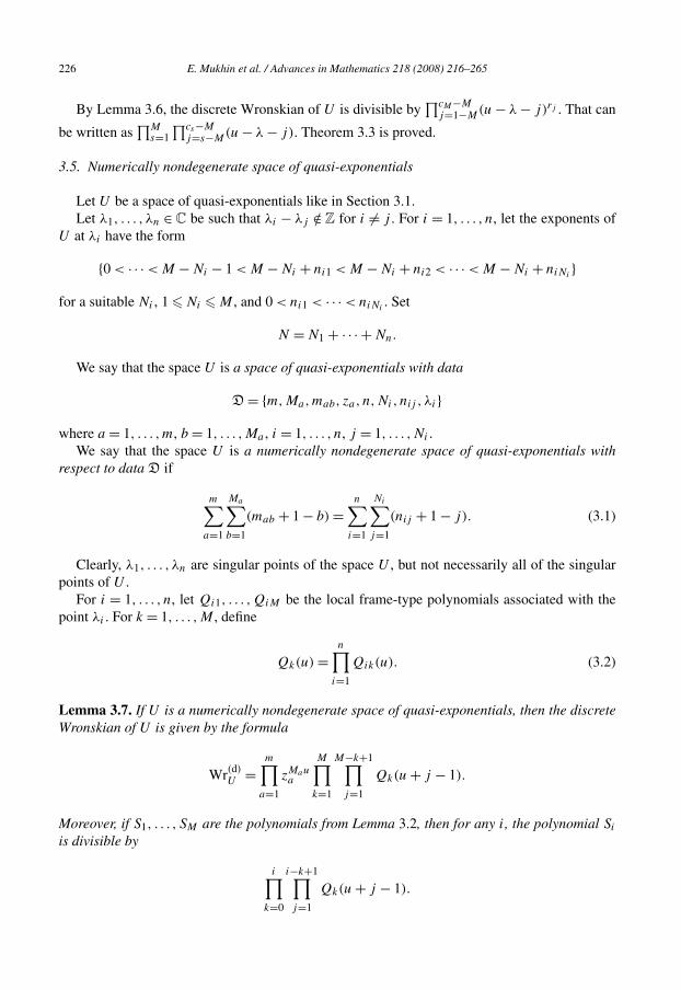
3.5. Numerically nondegenerate space of quasi-exponentials
Let U be a space of quasi-exponentials like in Section 3.1.Let λ1, . . . , λn ∈ C be such that λi − λj /∈ Z for i �= j . For i = 1, . . . , n, let the exponents of
U at λi have the form
{0 < · · · < M − Ni − 1 < M − Ni + ni1 < M − Ni + ni2 < · · · < M − Ni + niNi}
for a suitable Ni , 1 � Ni � M , and 0 < ni1 < · · · < niNi. Set
N = N1 + · · · + Nn.
We say that the space U is a space of quasi-exponentials with data
D = {m,Ma,mab, za, n,Ni, nij , λi}where a = 1, . . . ,m, b = 1, . . . ,Ma , i = 1, . . . , n, j = 1, . . . ,Ni .
We say that the space U is a numerically nondegenerate space of quasi-exponentials withrespect to data D if
m∑a=1
Ma∑b=1
(mab + 1 − b) =n∑
i=1
Ni∑j=1
(nij + 1 − j). (3.1)
Clearly, λ1, . . . , λn are singular points of the space U , but not necessarily all of the singularpoints of U .
For i = 1, . . . , n, let Qi1, . . . ,QiM be the local frame-type polynomials associated with thepoint λi . For k = 1, . . . ,M , define
Qk(u) =n∏
i=1
Qik(u). (3.2)
Lemma 3.7. If U is a numerically nondegenerate space of quasi-exponentials, then the discreteWronskian of U is given by the formula
Wr(d)U =
m∏a=1
zMaua
M∏k=1
M−k+1∏j=1
Qk(u + j − 1).
Moreover, if S1, . . . , SM are the polynomials from Lemma 3.2, then for any i, the polynomial Si
is divisible by
i∏k=0
i−k+1∏j=1
Qk(u + j − 1).

E. Mukhin et al. / Advances in Mathematics 218 (2008) 216–265 227
The lemma follows from Lemmas 3.1, 3.2, and Theorem 3.3.
3.6. Fundamental difference operator
The monic fundamental difference operator of a space of quasi-exponentials U is the uniquemonic linear difference operator
DU = τMu + B1τ
M−1u + · · · + BM−1τu + BM
of order M annihilating U . Here
Bi = (−1)iWr(d)
U,i
Wr(d)U
,
where Wr(d)U is the discrete Wronskian of a basis {f1, . . . , fM} of U , Wr(d)
U,i is the determinant ofthe M × M-matrix whose j th row is
fj (u), fj (u + 1), . . . , fj (u + N − i − 1), fj (u + N − i + 1), . . . , fj (u + N).
Clearly, B1, . . . , BM are rational functions.
Lemma 3.8. For any i, the function Bi has a limit as u tends to infinity. Denote this limit byBi(∞). Then
xM + B1(∞)xM−1 + · · · + BM(∞) =M∏
a=1
(x − za)Ma .
The proof is straightforward.
Lemma 3.9. For any i = 1, . . . ,M , the function
Bi(u)
n∏i=1
Ni∏j=1
(u − λi − nij + Ni)
is a polynomial.
Proof. Let λ be one of the points of the set {λ1, . . . , λn}. For such a λ, in the proof of Theo-rem 3.3, we defined the numbers dj and rj for j ∈ Z.
For j ∈ Z, define the new numbers pj as follows. Set pj = dj+1 for j � 0, and set pj =max(0, j + dj+1) for j < 0.
By the construction, we have pj � rj .
The reasons in the proof of Theorem 3.3 show that the discrete Wronskian Wr(d)U is divisible
by
X(u) =cM−M∏
(u − λ − j)rj .
j=1−M

228 E. Mukhin et al. / Advances in Mathematics 218 (2008) 216–265
Similar reasons show that for any k, the determinant Wr(d)U,k is divisible by
Y(u) =cM−M−1∏j=1−M
(u − λ − j)pj .
As at the end of the proof of Theorem 3.3, we have
X(u) =M∏
s=1
cs−M∏j=s−M
(u − λ − j) =M∏
s=1cs�s
cs−M∏j=s−M
(u − λ − j),
where in the second expression we excluded the empty products over j . Similarly,
Y(u) =M∏
s=1cs�s+1
cs−1−M∏j=s−M
(u − λ − j) =M∏
s=1cs�s
cs−1−M∏j=s−M
(u − λ − j),
where the first expression is analogous to the second expression for X(u), and the second ex-pression may contain certain empty products over j .
Using the second expressions for X(u) and Y(u), we get
X(u) = Y(u)
M∏s=1cs�s
(u − λ − cs + M). (3.3)
Now if λ = λi , we shall provide X(u) and Y(u) with index i. Calculating the product in (3.3)for λ = λi , we get
Xi(u) = Yi(u)
Ni∏j=1
(u − λi − nij + Ni).
Multiplying this formula over i = 1, . . . , n, we conclude that for any k, the product
Wr(d)U,k(u)
n∏i=1
Ni∏j=1
(u − λi − nij + Ni)
is divisible by the discrete Wronskian Wr(d)U . �
Define the regularized fundamental difference operator of the space U as the linear differenceoperator
DU = B0(u)τMu + B1(u)τM−1
u + · · · + BM(u)
of order M with polynomial coefficients, which annihilates U and such that its leading coeffi-cient B0 is a monic polynomial of the minimal possible degree.
E. Mukhin et al. / Advances in Mathematics 218 (2008) 216–265 229
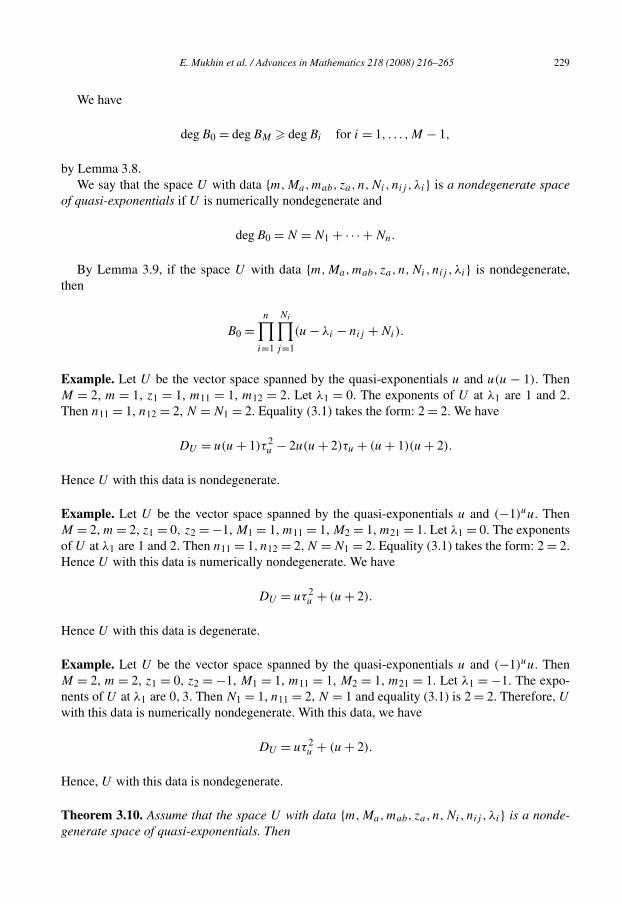
We have
degB0 = degBM � degBi for i = 1, . . . ,M − 1,
by Lemma 3.8.We say that the space U with data {m,Ma,mab, za, n,Ni, nij , λi} is a nondegenerate space
of quasi-exponentials if U is numerically nondegenerate and
degB0 = N = N1 + · · · + Nn.
By Lemma 3.9, if the space U with data {m,Ma,mab, za, n,Ni, nij , λi} is nondegenerate,then
B0 =n∏
i=1
Ni∏j=1
(u − λi − nij + Ni).
Example. Let U be the vector space spanned by the quasi-exponentials u and u(u − 1). ThenM = 2, m = 1, z1 = 1, m11 = 1, m12 = 2. Let λ1 = 0. The exponents of U at λ1 are 1 and 2.Then n11 = 1, n12 = 2, N = N1 = 2. Equality (3.1) takes the form: 2 = 2. We have
DU = u(u + 1)τ 2u − 2u(u + 2)τu + (u + 1)(u + 2).
Hence U with this data is nondegenerate.
Example. Let U be the vector space spanned by the quasi-exponentials u and (−1)uu. ThenM = 2, m = 2, z1 = 0, z2 = −1, M1 = 1, m11 = 1, M2 = 1, m21 = 1. Let λ1 = 0. The exponentsof U at λ1 are 1 and 2. Then n11 = 1, n12 = 2,N = N1 = 2. Equality (3.1) takes the form: 2 = 2.Hence U with this data is numerically nondegenerate. We have
DU = uτ 2u + (u + 2).
Hence U with this data is degenerate.
Example. Let U be the vector space spanned by the quasi-exponentials u and (−1)uu. ThenM = 2, m = 2, z1 = 0, z2 = −1, M1 = 1, m11 = 1, M2 = 1, m21 = 1. Let λ1 = −1. The expo-nents of U at λ1 are 0,3. Then N1 = 1, n11 = 2, N = 1 and equality (3.1) is 2 = 2. Therefore, U
with this data is numerically nondegenerate. With this data, we have
DU = uτ 2u + (u + 2).
Hence, U with this data is nondegenerate.
Theorem 3.10. Assume that the space U with data {m,Ma,mab, za, n,Ni, nij , λi} is a nonde-generate space of quasi-exponentials. Then

230 E. Mukhin et al. / Advances in Mathematics 218 (2008) 216–265
(i) We have
BM =m∏
a=1
(−za)Ma
n∏i=1
Ni∏j=1
(u − λi + j).
(ii) Write
DU = uNA0(τu) + uN−1A1(τu) + · · · + AN(τu)
where Ai(τu) is a polynomial in τu with constant coefficients. Then
A0(τu) =m∏
a=1
(τu − za)Ma .
(iii) The polynomials A0, . . . ,AM have no common factors of positive degree.
Corollary 3.11. If the space U is nondegenerate with respect to a data {m,Ma,mab, za, n,
Ni, nij , λi}, then the data is determined uniquely.
The corollary follows from part (i) of the theorem.
Proof of Theorem 3.10. Part (ii) follows from Lemma 3.8. Part (iii) follows from the fact thatU does not contain exponential functions zu.
Let Q1, . . . ,QM be the polynomials introduced in (3.2). To prove part (i) it is enough to noticethat
BM(u)
B0(u)= (−1)M
Wr(d)(u + 1)
Wr(d)(u)=
M∏k=1
Qk(u + M + 1 − k)
Qk(u)
m∏a=1
zMaa
= (−1)Mn∏
i=1
Ni∏j=1
u − λi + j
u − λi − nij + Ni
m∏a=1
zMaa . �
3.7. Regularized conjugate space
Let U with data {m,Ma,mab, za, n,Ni, nij , λi} be a nondegenerate space of quasi-exponen-
tials as in Section 3.6. Let Wr(d)U be the discrete Wronskian of U and let BM(u) be the last
coefficient of the regularized fundamental difference operator of U .The complex vector space spanned by all functions of the form
τu(Wr(d)(f1, . . . , fM−1))
BM(u)Wr(d)U (u)
(3.4)
with fi ∈ V has dimension M . This space is denoted by U‡ and called regularized conjugateto U .

E. Mukhin et al. / Advances in Mathematics 218 (2008) 216–265 231
Lemma 3.12. For any g ∈ U‡, the function
g(u)
n∏i=1
niNi∏j=0
(u − λi + Ni − j)
is holomorphic in C.
Proof. Let Q1, . . . ,QM be the polynomials introduced in (3.2). Let g be a function in (3.4).Then τu(Wr(d)(f1, . . . , fM−1)) is divisible by
M−1∏i=1
Q1(u + i) ·M−2∏i=1
Q2(u + i) · · ·QM−1(u + 1)
while
Wr(d)U (u) =
m∏a=1
zMaa
M∏j=1
Q1(u + j − 1) ·M−1∏j=1
Q2(u + j − 1) · · ·QM(u).
Hence, the possible poles of g come from the product BM(u)Q1(u) · · ·QM(u) which remains inthe denominator of g. But this product is exactly the product in Lemma 3.12. �
For every i = 1, . . . , n and j = 1, . . . ,Ni , fix a function gij in U which is equal to zero atu = λi, λi +1, . . . , λi +M −Ni +nij −1 and which is not equal to zero at u = λi +M −Ni +nij .
Lemma 3.13. For given i = 1, . . . , n, j = 0, . . . ,Ni − 1, let f1, . . . , fM−1 be a collection offunctions in U containing the functions gi,j+1, gi,j+2, . . . , gi,Ni
and let
F(u) = τu(Wr(d)(f1, . . . , fM−1))
BM(u)Wr(d)U (u)
.
Then for j = 0, the function F has no poles at
u = λi − Ni,λi − Ni + 1, . . . , λi − Ni + niNi.
For j > 0, the function F has no poles at
u = λi − Ni + nij + 1, λi − Ni + nij + 2, . . . , λi − Ni + niNi.
Moreover, if f1, . . . , fM−1 is a generic collection of functions in U containing the functionsgi,j+1, gi,j+2, . . . , gi,Ni
, then the function F has a nonzero residue at u = λi − Ni + nij .
Proof. The first two statements of the lemma are proved in the same way as Lemma 3.12.We shall prove that the residue of F at u = λi − Ni + nij is nonzero first assuming that
nij � Ni . To prove that the residue is nonzero it is enough to show that
ordu=λ −N +n Wr(d) = 1 + ordu=λ −N +n +1Wr(d) = Ni − j + 1, (3.5)
i i ij U i i ij U
232 E. Mukhin et al. / Advances in Mathematics 218 (2008) 216–265
and
ordu=λi−Ni+nij +1Wr(d)U = ordu=λi−Ni+nij +1Wr(d)(f1, . . . , fM−1). (3.6)
Here ordu=λf denotes the order of zero of the function f at u = λ.Equalities (3.5) follow from the numerical nondegeneracy of the space U and the condition
nij � Ni .Since the collection f1, . . . , fM−1 is a generic collection containing the functions gi,j+1,
. . . , gi,Ni, the discrete Wronskian Wr(d)(f1, . . . , fM−1, gij ) is nonzero and proportional to Wr(d)
U .Expanding the determinant Wr(d)(f1, . . . , fM−1, gij ) with respect to the last row, we have
Wr(d)U (u) = const
(gij (u + M − 1)Wr(d)(f1, . . . , fM−1)(u) − · · ·
− (−1)Mgij (u)τu
(Wr(d)(f1, . . . , fM−1)
)(u)
)(3.7)
where const �= 0.The order of Wr(d)(f1, . . . , fM−1) at u = λi − Ni + nij + 1 is not less than Ni − j . This
follows from Theorem 3.3 applied to the functions f1, . . . , fM−1. A similar reason shows thatthe order at u = λi −Ni +nij + 1 of all of the other (M − 1)× (M − 1) minors in the right-handside of (3.7) is also not less than Ni − j .
By the construction, the function gij is nonzero at u = λi − Ni + nij and is zero atu = λi − Ni + nij − l for l = 1, . . . ,M − 1. Therefore, the only term in the right-handside of equality (3.7) that can have order Ni − j at u = λi − Ni + nij + 1 is gij (u +M − 1)Wr(d)(f1, . . . , fM−1)(u). Since ordu=λi−Ni+nij +1Wr(d)
U = Ni − j , this shows that the or-
ders of Wr(d)U and Wr(d)(f1, . . . , fM−1) at u = λi − Ni + nij are equal.
To prove that the residue of F at u = λi − Ni + nij is nonzero in the case nij < Ni , it isenough to show that
ordu=λi−Ni+nijWr(d)
U = ordu=λi−Ni+nij +1Wr(d)U = nij − j + 1,
and
ordu=λi−Ni+nij +1Wr(d)U = ordu=λi−Ni+nij +1Wr(d)(f1, . . . , fM−1).
The proof is similar to the proof of equalities (3.5) and (3.6). �Theorem 3.14. If DU = B0(u)τM
u +B1(u)τM−1u + · · ·+ τuBM−1(u)+BM(u) is the regularized
fundamental difference operator of U , then the operator
D‡U = τM
u BM(u) + τM−1u BM−1(u) + · · · + τuB1(u) + B0(u)
annihilates U‡.
Proof. Consider the scalar equation DUy = 0 with respect to an unknown function y(u). Fori = 1, . . . ,M , introduce wi = τ i−1
u y and present the equation as a system of first order equations
τuwM = −B1(u)wM − · · · − BM(u)
w1, τuwi = wi+1
B0(u) B0(u)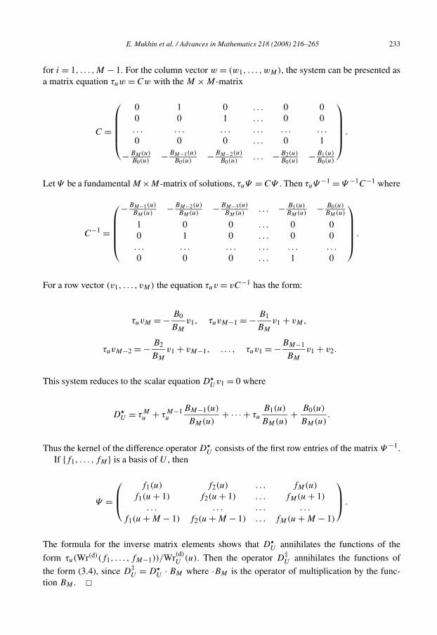
E. Mukhin et al. / Advances in Mathematics 218 (2008) 216–265 233
for i = 1, . . . ,M − 1. For the column vector w = (w1, . . . ,wM), the system can be presented asa matrix equation τuw = Cw with the M × M-matrix
C =
⎛⎜⎜⎜⎜⎝0 1 0 . . . 0 00 0 1 . . . 0 0. . . . . . . . . . . . . . . . . .
0 0 0 . . . 0 1
−BM(u)B0(u)
−BM−1(u)
B0(u)−BM−2(u)
B0(u). . . −B2(u)
B0(u)−B1(u)
B0(u)
⎞⎟⎟⎟⎟⎠ .
Let Ψ be a fundamental M ×M-matrix of solutions, τuΨ = CΨ . Then τuΨ−1 = Ψ −1C−1 where
C−1 =
⎛⎜⎜⎜⎜⎝−BM−1(u)
BM(u)−BM−2(u)
BM(u)−BM−3(u)
BM(u). . . − B1(u)
BM(u)− B0(u)
BM(u)
1 0 0 . . . 0 00 1 0 . . . 0 0. . . . . . . . . . . . . . . . . .
0 0 0 . . . 1 0
⎞⎟⎟⎟⎟⎠ .
For a row vector (v1, . . . , vM) the equation τuv = vC−1 has the form:
τuvM = − B0
BM
v1, τuvM−1 = − B1
BM
v1 + vM,
τuvM−2 = − B2
BM
v1 + vM−1, . . . , τuv1 = −BM−1
BM
v1 + v2.
This system reduces to the scalar equation D�Uv1 = 0 where
D�U = τM
u + τM−1u
BM−1(u)
BM(u)+ · · · + τu
B1(u)
BM(u)+ B0(u)
BM(u).
Thus the kernel of the difference operator D�U consists of the first row entries of the matrix Ψ −1.
If {f1, . . . , fM} is a basis of U , then
Ψ =⎛⎜⎝
f1(u) f2(u) . . . fM(u)
f1(u + 1) f2(u + 1) . . . fM(u + 1)
. . . . . . . . . . . .
f1(u + M − 1) f2(u + M − 1) . . . fM(u + M − 1)
⎞⎟⎠ .
The formula for the inverse matrix elements shows that D�U annihilates the functions of the
form τu(Wr(d)(f1, . . . , fM−1))/Wr(d)U (u). Then the operator D
‡U annihilates the functions of
the form (3.4), since D‡U = D�
U · BM where ·BM is the operator of multiplication by the func-tion BM . �

234 E. Mukhin et al. / Advances in Mathematics 218 (2008) 216–265
4. Integral transforms
4.1. Mellin-type transform
Let V be a nondegenerate space of quasi-polynomials with data DV = {n,Ni, nij , λi, m,Ma,
mab, za} where i = 1, . . . , n, j = 1, . . . ,Ni , a = 1, . . . ,m, b = 1, . . . ,Ma . Let V † be the regu-larized conjugate space to V .
For a = 1, . . . ,m, denote by γa a small circle around za in C oriented counterclockwise.Denote by U the complex vector space spanned by functions of the form
fa(u) =∫γa
xuf (x) dx, (4.1)
where a = 1, . . . ,m, f ∈ V †. The vector space U is called bispectral dual to V .
Theorem 4.1. Let V be a nondegenerate space of quasi-polynomials with data
DV = {n,Ni, nij , λi,m,Ma,mab, za}where i = 1, . . . , n, j = 1, . . . ,Ni , a= 1, . . . ,m, b = 1, . . . ,Ma . Then
(i) The space U is a nondegenerate space of quasi-exponentials with data
DU = {m,Ma,mab, za, n,Ni, nij , λi + Ni}where a = 1, . . . ,m, b = 1, . . . ,Ma , i = 1, . . . , n, j = 1, . . . ,Ni .
(ii) Let DV = ∑Mi=1
∑Nj=1 Aijx
i(x∂x)j be the regularized fundamental differential operator
of V where Aij are suitable complex numbers. Then
M∑i=1
N∑j=1
Aijuj τ i
u
is the regularized fundamental difference operator of U .
The theorem is proved in Section 4.3.
4.2. Fourier-type transform
Let U be a nondegenerate space of quasi-exponentials with data DU = {m,Ma,mab, za,
n,Ni, nij , λi} where a = 1, . . . ,m, b = 1, . . . ,Ma , i = 1, . . . , n, j = 1, . . . ,Ni . Let U‡ be theregularized conjugate space to U .
For i = 1, . . . , n, consider the arithmetic sequence
Si = {λi − Ni,λi − Ni + 1, λi − Ni + 2, . . . , λi − Ni + niNi}
consisting of niN + 1 terms.
i
E. Mukhin et al. / Advances in Mathematics 218 (2008) 216–265 235
For i = 1, . . . , n, fix a non-selfintersecting closed connected curve γi in C oriented coun-terclockwise and such that the points of the sequence Si are inside γi and the points of othersequences Sj for j �= i are outside γi .
Denote by V the complex vector space spanned by functions of the form
fi (x) =∫γi
xuf (u)du, (4.2)
where i = 1, . . . , n, f ∈ U‡. The vector space V is called bispectral dual to U .
Theorem 4.2. Let U be a nondegenerate space of quasi-exponentials with data
DU = {m,Ma,mab, za, n,Ni, nij , λi}
where a = 1, . . . ,m, b = 1, . . . ,Ma , i = 1, . . . , n, j = 1, . . . ,Ni . Then
(i) The space V is a nondegenerate space of quasi-polynomials with data
DV = {n,Ni, nij , λi − Ni,m,Ma,mab, za}
where i = 1, . . . , n, j = 1, . . . ,Ni , a = 1, . . . ,m, b = 1, . . . ,Ma .(ii) Let DU = ∑N
i=1∑M
j=1 Aijuiτ
ju be the regularized fundamental difference operator of U
where Aij are suitable complex numbers. Then
N∑i=1
M∑j=1
Aijxj (x∂x)
i
is the regularized fundamental differential operator of V .
The theorem is proved in Section 4.4.Theorems 4.1 and 4.2 imply that if V is a nondegenerate space of quasi-polynomials and U
is bispectral dual to V , then V is bispectral dual to U . Similarly, if U is a nondegenerate spaceof quasi-exponentials and V is bispectral dual to U , then U is bispectral dual to U .
4.3. Proof of Theorem 4.1
The exponents of V † at za are
{−ma,Ma − 1 < · · · < −ma1 − 1 < 0 < 1 < · · · < N − Ma − 1}.
Integral (4.1) is nonzero only if f has a pole at x = za . If f has a pole at x = za of order−mab −1, then integral (4.1) has the form zu
aqab(u) where qab is a polynomial in u of degree mab .Thus U is a space of quasi-exponentials of dimension M generated by quasi-exponentialszuqab(u) where a = 1, . . . ,m, b = 1, . . . ,mab and qab is a polynomial in u of degree mab .
a
236 E. Mukhin et al. / Advances in Mathematics 218 (2008) 216–265
It is clear that the operator D† = ∑Mi=1
∑Nj=1 Aiju
j τ iu annihilates U . Write
D† = B0(u)τMu + · · · + BM−1(u)τu + BM(u)
where Ba(u) are polynomials in u with constant coefficients. Lemma 2.3 implies that B0(u) =∏nj=1(u − λj )
Nj and the polynomials B0, . . . ,BM have no common factor of positive degree.
Therefore, D† is the regularized fundamental operator of U .The functions xλi pij (x), i = 1, . . . , n, j = 1, . . . ,Ni , form a basis of V . For given i, j , order
all basis functions of V except the function xλi pij (x). Denote by Wrij the Wronskian of thisordered set of N − 1 functions. The functions
fij (x) = Wrij (x)
WrV (x)xN∏m
a=1(x − za)Ma
form a basis in V †. Such a function fij has the form x−λi rij where rij is a rational function in x.We have
ordx=0rij = −Ni, ordx=∞rij = −nij − M − 1.
Consider the following element of U ,
Fij (u) =m∑
a=1
(fij )a(u) =∫
⋃ma=1 γa
xufij (x) dx.
If u = λi + m whereNi � m � nij + M − 1, then the integrand is a rational function with zeroresidues at 0 and ∞. Hence Fij is zero at u = λi + m for m from this arithmetic sequence. Thisremark together with Theorem 3.3 proves that U is a nondegenerate space of quasi-exponentialswith data {m,Ma,mab, za, n,Ni, nij , λi + Ni}.
4.4. Proof of Theorem 4.2
By Lemmas 3.12 and 3.13, for any i = 1, . . . , n, the functions fi (x) in (4.2) have the formxλi−Ni pij (x) where j = 1, . . . ,Ni and pij is a polynomial of degree not greater than nij . More-over, there exists a function xλi−Ni pij (x) with pij of degree exactly equal to nij .
The functions zuaqab(u), a = 1, . . . ,m, b = 1, . . . ,Ma , form a basis of U . For given a, b,
order all basis functions of U except the function zuaqab(u) and denote them f1, . . . , fM−1. The
corresponding function
fab(u) = τu(Wr(d)(f1, . . . , fM−1))
BM(u)Wr(d)U (u)
∈ U‡
has the form z−ua rab(u) where rab is a rational function in u and ordu=∞rab = Ma −mab −N −1.
Consider the following element of V ,
Fab(x) =n∑
i=1
(fab)i(x) =∫
⋃n γ
xufij (u) du.
i=1 i

E. Mukhin et al. / Advances in Mathematics 218 (2008) 216–265 237
If x = za , then the integrand is a rational function in u which tends to zero as u tends to infinity.Denote by (i) the ith derivative. Then F
(i)ab (za) = 0 for i = 0,1, . . . ,N − Ma + mab − 1, and
F(N−Ma+mab)ab (za) �= 0.
This reason proves part (i) of the theorem.From Theorem 3.14 and formulas for the Fourier-type integral transform, it follows that the
differential operator∑N
i=1∑M
j=1 Aijxj (x∂x)
i annihilates V . From part (iii) of Theorem 3.10, itfollows that this operator is the regularized fundamental differential operator of V .
5. Rigged spaces
In this section we consider special spaces of quasi-polynomials and quasi-exponentials withadditional structures. We call such spaces rigged spaces.
5.1. Spaces of quasi-polynomials of (n,λ,m,z)-type
Let N be a natural number, N > 1. Let n = (n1, . . . , nN) be a vector of nonnegative integers.Let λ = (λ1, . . . , λN) ∈ CN . Assume that λi − λj /∈ Z for i �= j .For i = 1, . . . ,N , let pi ∈ C[x] be a polynomial of degree ni such that pi(0) �= 0. Denote
by V the complex vector space spanned by functions xλi pi(x), i = 1, . . . ,N . The dimensionof V is N .
Let z = (z1, . . . , zM), M > 1, be a subset in C containing all singular points of V . Assumethat for a = 1, . . . ,M , the set of exponents of V at za has the form
{0 < 1 < · · · < N − 2 < N − 1 + ma}, ma � 0.
We have
N∑i=1
ni =M∑
a=1
ma.
We call the pair (V ,z) a space of (n,λ,m,z)-type or a rigged space of quasi-polynomials.Let DV be the monic fundamental differential operator of V . The operator
DV = xNM∏
a=1
(x − za)DV
is called the rigged fundamental differential operator of the rigged space (V ,z).Write the rigged fundamental differential operator in the form
DV = A0(x)(x∂x)N + A1(x)(x∂x)
N−1 + A2(x)(x∂x)N−2 + · · · + AN(x).
Then by Lemma 2.3, all of the coefficients A0, . . . ,AN are polynomials in x of degree not greaterthan M . If we write
DV = xMB0(x∂x) + xM−1B1(x∂x) + · · · + xBM−1(x∂x) + BM(x∂x),

238 E. Mukhin et al. / Advances in Mathematics 218 (2008) 216–265
where Bi is a polynomial in x∂x with constant coefficients, then
B0 =N∏
i=1
(x∂x − λi − ni), BM = (−1)MM∏
a=1
za
N∏i=1
(x∂x − λi).
Note that a space V of (n,λ,m,z)-type may contain a function of the form xλi and be adegenerate space of quasi-polynomials in the sense of Section 2.1. Note also that the subset z
may contain nonsingular points of V and then the rigged fundamental differential operator DV
differs from the regularized differential operator of the space V .
5.2. Spaces of quasi-exponentials of (m,z,n,λ)-type
Let M be a natural number, M > 1. Let m = (m1, . . . ,mM) be a vector of nonnegative inte-gers.
Let z = (z1, . . . , zM) be distinct nonzero complex numbers with fixed arguments.For a = 1, . . . ,M , let qa ∈ C[u] be a polynomial of degree ma . Denote by U the complex
vector space spanned by the functions zuaqa(u), a = 1, . . . ,M . The dimension of U is M .
Assume that for some natural number N > 1, there exists a subset of distinct numbers λ =(λ1, . . . , λN) in C with three properties:
• λi − λj /∈ Z for i �= j .• For i = 1, . . . ,N , the set of discrete exponents of U at λi has the form
{0 < 1 < · · · < M − 2 < M − 1 + ni}, ni � 0.
• ∑Ni=1 ni = ∑M
a=1 ma .
In this case we call the pair (U,λ) a space of quasi-exponentials of (m,z,n,λ)-type or a riggedspace of quasi-exponentials.
Let DU be the monic fundamental difference operator of U . The operator
DU =N∏
i=1
(u − λi − ni + 1)DV
is called the rigged fundamental difference operator of the rigged space (U,λ).Write the rigged fundamental difference operator in the form
DU = B0(u)τMu + B1(u)τM−1
u + B2(u)τM−2u + · · · + BM(u).
Lemma 3.9 and Theorem 3.10 may be applied to the space U and we conclude that all of thecoefficients B0, . . . ,BM are polynomials in u of degree not greater than N and
BM = (−1)MM∏
za
N∏(u − λi + 1).
a=1 i=1

E. Mukhin et al. / Advances in Mathematics 218 (2008) 216–265 239
If we write
DU = uNA0(τu) + uN−1A1(τu) + · · · + uAN−1(τu) + AN(τu),
where Ai(τu) is a polynomial in τu with constant coefficients, then
A0(τu) =M∏
a=1
(τu − za).
Note that a space U of (m,z,n,λ)-type may contain a function of the form zua and be not a
space of quasi-exponentials in the sense of Section 3.1. Note also that the subset λ may containpoints λi with ni = 0 and then the rigged fundamental difference operator DU differs from theregularized difference operator of the space U .
5.3. Rigged Mellin-type transform
Let (V ,z) be a space of quasi-polynomials of an (n,λ,m,z)-type. Let V � be the space con-jugate to V and defined in Section 2.4.
For a = 1, . . . ,M , let γa be a small circle around za in C oriented counterclockwise. Denoteby U the complex vector space spanned by the functions of the form
fa(u) =∫γa
xuf (x)x−NM∏
a=1
(x − za)−1 dx, (5.1)
where a = 1, . . . ,M , f ∈ V �.
Theorem 5.1. Let (V ,z) be a space of quasi-polynomials of an (n, (λ1, . . . , λN),m,
(z1, . . . , zM))-type. Then
(i) The space U is a space of quasi-exponentials of the (m, (z1, . . . , zN),n, (λ1 + 1, . . . ,
λN + 1))-type.(ii) Let DV = ∑M
i=1∑N
j=1 Aijxi(x∂x)
j be the rigged fundamental differential operator of V
where Aij are suitable complex numbers. Then
M∑i=1
N∑j=1
Aijuj τ i
u
is the rigged fundamental difference operator of U .
The proof is similar to the proof of Theorem 4.1.The rigged space of quasi-exponentials (U, (λ1 + 1, . . . , λN + 1)) is called rigged bispectral
dual to the rigged space of quasi-polynomials (V ,z).

240 E. Mukhin et al. / Advances in Mathematics 218 (2008) 216–265
5.4. Rigged Fourier-type transform
Let (U,λ) be a space of quasi-exponentials of an (m,z,n,λ)-type. Let Wr(d)U be the discrete
Wronskian of U and let BM(u) be the last coefficient of the rigged fundamental difference oper-ator of U .
The complex vector space spanned by all functions of the form
τu(Wr(d)(f1, . . . , fM−1))
BM(u)Wr(d)U (u)
(5.2)
with fi ∈ V has dimension M . This space is denoted by U• and called rigged regularized conju-gate to U .
For i = 1, . . . ,N , consider the arithmetic sequence
Si = {λi − 1, λi, λi + 1, . . . , λi + ni − 1}consisting of ni + 1 terms.
For i = 1, . . . ,N , fix a non-selfintersecting closed connected curve γi in C oriented counter-clockwise such that it encircles the sequence Si and does not contain inside or intersect withpoints of other sequences Sj for j �= i.
Denote by V the complex vector space spanned by functions of the form
fi (x) =∫γi
xuf (u)du,
where i = 1, . . . , n, f ∈ U•.
Theorem 5.2. Let (U,λ) be a space of quasi-exponentials of an (m, (z1, . . . , zM),n,
(λ1, . . . , λN))-type. Then
(i) The space V is a space of quasi-exponentials of the (n, (λ1 − 1, . . . , λN − 1),m,
(z1, . . . , zN))-type.(ii) Let Du = ∑M
i=1∑N
j=1 Aijuiτ
ju be the rigged fundamental difference operator of U where
Aij are suitable complex numbers. Then
M∑i=1
N∑j=1
Aijxj (x∂x)
i
is the rigged fundamental differential operator of V .
The proof is similar to the proof of Theorem 4.2.The rigged space of quasi-polynomials (V ,z) is called rigged bispectral dual to the rigged
space of quasi-exponentials (U,λ).Theorems 5.1 and 5.2 imply that if V is a rigged space of quasi-polynomials and U is rigged
bispectral dual to V , then V is rigged bispectral dual to U . Similarly, if U is a rigged space ofquasi-exponentials and V is rigged bispectral dual to U , then U is rigged bispectral dual to U .

E. Mukhin et al. / Advances in Mathematics 218 (2008) 216–265 241
6. Rigged spaces and solutions of the Bethe ansatz equations
6.1. Critical points of master functions and rigged spaces of quasi-polynomials
Let (V ,z) be a space of quasi-polynomials of an (n,λ,m,z)-type. We construct the associatedmaster function as follows. Set
ni = ni+1 + · · · + nN, i = 1, . . . ,N − 1.
Consider the new n1 + · · · + nN−1 auxiliary variables
t 〈n〉 = (t(1)1 , . . . , t
(1)n1
, t(2)1 , . . . , t
(2)n2
, . . . , t(N−1)1 , . . . , t
(N−1)nN−1
).
Define the master function
Φ(t 〈n〉;λ;m;z) =
M∏a=1
zma(λ1+ma/2)a
∏1�a<b�M
(za − zb)mamb
N∏i=1
ni∏j=1
(t(i)j
)λi+1−λi+1
×M∏
a=1
n1∏j=1
(t(1)j − za
)−ma
N−1∏i=1
∏j<j ′
(t(i)j − t
(i)
j ′)2
×N−2∏i=1
ni∏j=1
ni+1∏j ′=1
(t(i)j − t
(i+1)
j ′)−1
. (6.1)
The master function is symmetric with respect to the group Σn = Σn1 × · · · × ΣnN−1 of permu-
tations of variables t(i)j preserving the upper index.
A point t 〈n〉 with complex coordinates is called a critical point of Φ(·;λ;m;z) if(Φ−1 ∂Φ
∂t(i)j
)(t 〈n〉;λ;m;z) = 0, i = 1, . . . ,N − 1, j = 1, . . . , ni .
In other words, a point t 〈n〉 is a critical point if the following system of n1 +· · ·+ nN−1 equationsis satisfied
λ1 − λ2 − 1
t(1)j
+M∑
a=1
ma
t(1)j − za
−n1∑
j ′=1, j ′ �=j
2
t(1)j − t
(1)
j ′+
n2∑j ′=1
1
t(1)j − t
(2)
j ′= 0,
λi − λi+1 − 1
t(i)j
−ni∑
j ′=1, j ′ �=j
2
t(i)j − t
(i)
j ′+
ni−1∑j ′=1
1
t(i)j − t
(i−1)
j ′+
ni+1∑j ′=1
1
t(i)j − t
(i+1)
j ′= 0,
λN−1 − λN − 1
t(N−1)
−nN−1∑
′ ′
2
t(N−1) − t
(N−1)′
+nN−2∑
′
1
t(N−1) − t
(N−2)′
= 0, (6.2)
j j =1, j �=j j j j =1 j j
242 E. Mukhin et al. / Advances in Mathematics 218 (2008) 216–265
where j = 1, . . . , n1 in the first group of equations, i = 2, . . . ,N − 2 and j = 1, . . . , ni in thesecond group of equations, j = 1, . . . , nN−1 in the last group of equations.
In the Gaudin model, Eqs. (6.2) are called the Gaudin Bethe ansatz equations.The Σn-orbit of a point t 〈n〉 ∈ Cn1+···+nN−1 is uniquely determined by the N −1-tuple yt 〈n〉 =
(y1, . . . , yN−1) of polynomials in x, where
yi =ni∏
j=1
(x − t
(i)j
), i = 1, . . . ,N − 1.
We say that y represents the orbit. Each polynomial of the tuple is considered up to multiplicationby a nonzero number since we are interested in the roots of the polynomial only.
We say that t 〈n〉 ∈ Cn1+···+nN−1 is Gaudin admissible if the value Φ(t 〈n〉;λ;m;z) is welldefined and is not zero.
A point t 〈n〉 is Gaudin admissible if and only if the associated tuple has the following proper-ties.
• For a = 1, . . . ,M , if ma > 0, then y1(za) �= 0.• For all i, yi(0) �= 0.• For all i, the polynomial yi has no multiple roots and no common roots with yi−1 or yi+1.
Such tuples are called Gaudin admissible.
Return to (V ,z), a space of an (n,λ,m,z)-type.The space V = 〈xλ1p1(x), . . . , xλN pN(x)〉 determines the N − 1-tuple yV = (y1, . . . , yN−1)
of polynomials in x, where
yN−1 = pN, yi = x(N−i)(N−i−1)
2 −λi+1−···−λN Wr(xλi+1pi+1(x), . . . , xλN pN(x)
)for i = 1, . . . ,N − 2.
We call the rigged space (V ,z) Gaudin admissible if the tuple yV is Gaudin admissible.
Theorem 6.1. (See [15,17].)
(i) Assume that the rigged space (V ,z) is Gaudin admissible. Then the tuple yV represents theorbit of a critical point of the master function.
(ii) Assume that t 〈n〉 is Gaudin admissible and t 〈n〉 is a critical point of the master function. Lety = (y1, . . . , yN−1) be the tuple representing the orbit of t 〈n〉. Then the differential operator
D =(
∂x − ln′(
xλ1−N+1 ∏Ma=1(x − za)
ma
y1
))(∂x − ln′
(xλ2−N+2y1
y2
)). . .
(∂x − ln′
(xλN−1−1yN−2
yN−1
))(∂x − ln′(xλN yN−1
))of order N is the monic fundamental differential operator of a Gaudin admissible riggedspace of quasi-polynomials (V ,z) of the (n,λ,m,z)-type.

E. Mukhin et al. / Advances in Mathematics 218 (2008) 216–265 243
(iii) The correspondence between Gaudin admissible rigged spaces of quasi-polynomials of the(n,λ,m,z)-type and orbits of Gaudin admissible critical points of the master function de-scribed in parts (i), (ii) is reflexive.
This theorem establishes a one-to-one correspondence between Gaudin admissible riggedspaces of quasi-polynomials of (n,λ,m,z)-type and orbits of Gaudin admissible critical pointsof the master function.
6.2. Solutions of the Bethe ansatz equations and rigged spaces of quasi-exponentials
Let (U,λ) be a space of quasi-exponentials of an (m,z,n,λ)-type. We define the associatedsystem of Bethe ansatz equations as follows. Set
ma = ma+1 + · · · + mM, a = 1, . . . ,M − 1.
Consider the new m1 + · · · + mM−1 auxiliary variables
t 〈m〉 = (t(1)1 , . . . , t
(1)m1
, t(2)1 , . . . , t
(2)m2
, . . . , t(M−1)1 , . . . , t
(M−1)mM−1
).
The Bethe ansatz equations of the XXX model is the following system of m1 + · · · + mM−1equations:
N∏i=1
t(1)b − λi
t(1)b − λi − ni
∏b′ �=b
t(1)b − t
(1)
b′ − 1
t(1)b − t
(1)
b′ + 1
m2∏b′=1
t(1)b − t
(2)
b′ + 1
t(1)b − t
(2)
b′= z2
z1,
ma−1∏b′=1
t(a)b − t
(a−1)
b′
t(a)b − t
(a−1)
b′ − 1
∏b′ �=b
t(a)b − t
(a)
b′ − 1
t(a)b − t
(a)
b′ + 1
ma+1∏b′=1
t(a)b − t
(a+1)
b′ + 1
t(a)b − t
(a+1)
b′= za+1
za
,
mN−2∏b′=1
t(N−1)b − t
(N−2)
b′
t(N−1)b − t
(N−2)
b′ − 1
∏b′ �=b
t(N−1)b − t
(N−1)
b′ − 1
t(N−1)b − t
(N−1)
b′ + 1= zM
zM−1(6.3)
where b = 1, . . . , m1 in the first group of equations, a = 2, . . . ,M − 2 and b = 1, . . . , ma in thesecond group of equations, b = 1, . . . , mM−1 in the last group of equations.
The system of Bethe ansatz equations is symmetric with respect to the groupΣm = Σm1 × · · · × ΣmM−1 of permutations of variables t
(a)b preserving the upper index.
The Σm-orbit of a point t 〈m〉 ∈ Cm1+···+mM−1 is uniquely determined by the M − 1-tupleyt 〈m〉 = (y1, . . . , yM−1) of polynomials in u, where
ya =ma∏b=1
(u − t
(a)b
), a = 1, . . . ,M − 1.
We say that y represents the orbit. Each polynomial of the tuple is considered up to multiplicationby a nonzero number.
We say that t 〈m〉 ∈ Cm1+···+mM−1 is XXX admissible of λ-type if

244 E. Mukhin et al. / Advances in Mathematics 218 (2008) 216–265
t(a)b �= t
(a)
b′ , t(a)b �= t
(a)
b′ + 1, t(a)b �= t
(a+1)
b′ , t(a)b �= t
(a+1)
b′ − 1,
t(1)b �= λi + r,
for all a, b, b′, i, and r = 0, . . . , ni .If t 〈m〉 ∈ Cm1+···+mM−1 is XXX admissible, then the corresponding tuple yt 〈m〉
is called XXXadmissible.
Return to (U,λ), a rigged space of quasi-exponentials of an (m,z,n,λ)-type.The space U = 〈zu
1q1(u), . . . , zuMqM(u)〉 determines the M −1-tuple yU = (y1, . . . , yM−1) of
polynomials in u, where
yM−1 = qM, ya =M∏
b=a+1
z−ub Wr(d)
(zua+1qa+1(u), . . . , zu
MqM(u))
for a = 1, . . . ,M − 2.We call the rigged space (U,λ) XXX admissible if the tuple yU is XXX admissible.
Theorem 6.2. (See [14,17].)
(i) Assume that the rigged space (U,λ) is XXX admissible. Then the tuple yU represents theorbit of a solution of the XXX Bethe ansatz equations (6.3).
(ii) Assume that t 〈m〉 is XXX admissible and t 〈m〉 is a solution of the XXX Bethe ansatz equa-tions (6.3). Let y = (y1, . . . , yM−1) be the tuple representing the orbit of t 〈m〉. Then thedifference operator
D =(
τu − y1(u)
y1(u + 1)
N∏i=1
u − λi + 1
u − λi − ni + 1z1
)(τu − y1(u + 1)
y1(u)
y2(u)
y2(u + 1)z2
)
. . .
(τu − yM−2(u + 1)
yM−2(u)
yM−1(u)
yM−1(u + 1)zM−1
)(τu − yM−1(u + 1)
yM−1(u)zM
)of order M is the monic fundamental difference operator of a rigged space of quasi-exponentials (U,λ) of (m,z,n,λ)-type.
(iii) The correspondence between XXX admissible rigged spaces of quasi-exponentials of the(m,z,n,λ)-type and orbits of XXX admissible solutions of the XXX Bethe ansatz equationsdescribed in parts (i), (ii) is reflexive.
This theorem establishes a one-to-one correspondence between XXX admissible riggedspaces of quasi-exponentials of (m,z,n,λ)-type and orbits of XXX admissible solutions of theXXX Bethe ansatz equations.
7. Finiteness of solutions of the Bethe ansatz equations
7.1. Finiteness of the Gaudin admissible critical points
Lemma 7.1. For given fixed m, z and generic λ, the master function Φ(t 〈n〉;λ;m;z), defined in(6.1), has only finitely many Gaudin admissible critical points.

E. Mukhin et al. / Advances in Mathematics 218 (2008) 216–265 245
The lemma follows from Lemma 2.1 in [15].
7.2. The number of orbits of the Gaudin admissible critical points
Let λ1, . . . , λN ∈ C be distinct numbers such that λi −λj /∈ Z for i �= j . Set n = n1 +· · ·+nN .Consider the complex vector space X spanned by functions xλi+j , i = 1, . . . ,N , j = 0, . . . , ni .The space X is of dimension n + N .
For z ∈ C∗, define a complete flag F (z) in X,
F (z) = {0 = F0(z) ⊂ F1(z) ⊂ · · · ⊂ Fn+N(z) = X
},
where Fk(z) consists of all f ∈ X which have zero at z of order not less that n + N − k. Thesubspace Fk(z) has dimension k.
Define two complete flags of X at infinity.Say that xλi+j <1 xλi′+j ′
if i < i′ or i = i′ and j < j ′. Set
F (∞1) = {0 = F0(∞1) ⊂ F1(∞1) ⊂ · · · ⊂ Fn+N(∞1) = X
},
where Fk(∞1) is spanned by k smallest elements with respect to <1.Say that xλi+j <2 xλi′+j ′
if i > i′ or i = i′ and j < j ′. Set
F (∞2) = {0 = F0(∞2) ⊂ F1(∞2) ⊂ · · · ⊂ Fn+N(∞2) = X
},
where Fk(∞2) is spanned by k smallest elements with respect to <2.Denote by Gr(X,N) the Grassmannian manifold of N -dimensional vector subspaces of X.
Let F be a complete flag of X,
F = {0 = F0 ⊂ F1 ⊂ · · · ⊂ Fn+N = X}.
A ramification sequence is a sequence (c1, . . . , cN) ∈ ZN such that n � c1 � · · · � cN � 0. For aramification sequence c = (c1, . . . , cN) define the Schubert cell
Ωoc (F ) = {
V ∈ Gr(X,N)∣∣ dim(V ∩ Fu) = �,
n + � − c� � u < n + � + 1 − c�+1, � = 0, . . . ,N},
where c0 = n, cN+1 = 0. The cell Ωoc (F ) is a smooth connected variety. The closure of Ωo
c (F )
is denoted by Ωc(F ). The codimension of Ωoc (F ) is
|c| = c1 + c2 + · · · + cN .
Every N -dimensional vector subspace of X belongs to a unique Schubert cell Ωoc (F ).
For a = 1, . . . ,M , define the ramification sequence
c(a) = (ma,0, . . . ,0).
Define the ramification sequences

246 E. Mukhin et al. / Advances in Mathematics 218 (2008) 216–265
c(∞1) = (n2 + · · · + nN,n3 + · · · + nN, . . . , nN ,0),
c(∞2) = (n1 + · · · + nN−1, n1 + · · · + nN−2, . . . , n1,0).
Lemma 7.2.
• We have
M∑a=1
codimΩoc(a)
(F (za)
) + codimΩoc(∞1)
(F (∞1)
) + codimΩoc(∞2)
(F (∞2)
)= dim Gr(X,N) = Nn.
• Let V ∈ Gr(X,N). The pair (V ,z) is a space of the (n,λ,m,z)-type, if and only if V belongsto the intersection of M + 2 Schubert cells
Ωoc(1)
(F (z1)
) ∩ Ωoc(2)
(F (z2)
) ∩ · · ·∩ Ωo
c(M)
(F (zM)
) ∩ Ωoc(∞1)
(F (∞1)
) ∩ Ωoc(∞2)
(F (∞2)
).
The proof is straightforward.According to Schubert calculus, the multiplicity of the intersection of Schubert cycles
Ωc(1)
(F (z1)
) ∩ Ωc(2)
(F (z2)
) ∩ · · ·∩ Ωc(M)
(F (zM)
) ∩ Ωc(∞1)
(F (∞1)
) ∩ Ωc(∞2)
(F (∞2)
)(7.1)
can be expressed in representation-theoretic terms as follows.For a ramification sequence c denote by L
〈N〉c the finite-dimensional irreducible glN -module
with highest weight c. Any glN -module L〈N〉 has a natural structure of an slN -module denotedby L〈N〉. By [5], the multiplicity of the intersection in (7.1) is equal to the multiplicity of thetrivial slN -module in the tensor product of slN -modules
L〈N〉c(1) ⊗ · · · ⊗ L
〈N〉c(M) ⊗ L
〈N〉c(∞1)
⊗ L〈N〉c(∞2)
. (7.2)
Proposition 7.3. (See [11].) The multiplicity of the trivial slN -module in the tensor product (7.2)
is equal to the dimension of the weight subspace of weight [n1, . . . , nN ] in the tensor product ofglN -modules
L〈N〉c(1) ⊗ · · · ⊗ L
〈N〉c(M). (7.3)
Corollary 7.4. For generic λ, the number of orbits of the Gaudin admissible critical pointsof the master function Φ(t 〈n〉;λ;m;z), is not greater than the dimension of the weight space(L
〈N〉c(1) ⊗ · · · ⊗ L
〈N〉c(M))[n1, . . . , nN ].

E. Mukhin et al. / Advances in Mathematics 218 (2008) 216–265 247
7.3. Finiteness of solutions of Bethe ansatz equations (6.3)
Let z = (z1, . . . , zM) ∈ CM . Let (m1, . . . , mM−1) be a collection of nonnegative integers. Wesay that z is separating with respect to (m1, . . . , mM−1) if
M−1∏a=1
(za+1
za
)ca
�= 1
for all sets of integers {c1, . . . , cM−1} such that 0 � ca � ma ,∑
a ca > 0.Clearly, for given (m1, . . . , mM−1), a generic z is separating.
Lemma 7.5. Let n, λ, (m1, . . . , mM−1) be fixed. Let z be separating with respect to(m1, . . . , mM−1). Then the Bethe ansatz equations (6.3) have only finitely many XXX admis-sible solutions of λ-type.
Proof. If the algebraic set of XXX admissible solutions of (6.3) is infinite, then it is unbounded.Suppose that we have a sequence of solutions which is unbounded. Without loss of generality,we assume that t
(a)b tends to infinity for a = 1, . . . ,M − 1, b = 1, . . . , ca , and remains bounded
for all other values of a, b. Multiply all of the equations in (6.3) corresponding to a variables t(a)b
with a = 1, . . . ,M − 1, b = 1, . . . , ca , and pass in the product to the limit along our sequence ofsolutions. Then the resulting equation is
M−1∏a=1
(za+1
za
)ca
= 1.
This equation contradicts to our assumption. �7.4. The number of orbits of the XXX admissible solutions
Let z1, . . . , zM ∈ C be distinct numbers with fixed argument. Set m = m1 + · · · + mM . Con-sider the complex vector space Y spanned by functions zu
aub , a = 1, . . . ,M , b = 0, . . . ,ma . The
space Y is of dimension m + M .For λ ∈ C, define a complete flag F (λ) in Y ,
F (λ) = {0 = F0(λ) ⊂ F1(λ) ⊂ · · · ⊂ Fm+M(λ) = Y
},
where Fk(λ) consists of all f ∈ Y which are divisible by∏m+M−k
j=1 (u−λ− j +1). The subspaceFk(λ) has dimension k.
Define two complete flags of Y at infinity.Say that zu
aub <1 zu
a′ub′if a < a′ or a = a′ and b < b′. Set
F (∞1) = {0 = F0(∞1) ⊂ F1(∞1) ⊂ · · · ⊂ Fm+M(∞1) = Y
},
where Fk(∞1) is spanned by k smallest elements with respect to <1.

248 E. Mukhin et al. / Advances in Mathematics 218 (2008) 216–265
Say that zuau
b <2 zua′ub′
if a > a′ or a = a′ and b < b′. Set
F (∞2) = {0 = F0(∞2) ⊂ F1(∞2) ⊂ · · · ⊂ Fm+M(∞2) = Y
},
where Fk(∞2) is spanned by k smallest elements with respect to <2.Denote by Gr(Y,M) the Grassmannian manifold of M-dimensional vector subspaces of Y .
Let F be a complete flag of Y ,
F = {0 = F0 ⊂ F1 ⊂ · · · ⊂ Fm+M = Y
}.
For a ramification sequence c = (c1, . . . , cM) ∈ ZM , m � c1 � · · · � cM � 0, denote byΩo
c (F ) ⊂ Gr(Y,M) the corresponding Schubert cell.For i = 1, . . . ,N , define the ramification sequence
c(i) = (ni,0, . . . ,0).
Define the ramification sequences
c(∞1) = (m2 + · · · + mM,m3 + · · · + mM, . . . ,mM,0),
c(∞2) = (m1 + · · · + mM−1,m1 + · · · + mM−2, . . . ,m1,0).
Lemma 7.6.
• We have
N∑i=1
codimΩoc(i)
(F (λi)
) + codimΩoc(∞1)
(F (∞1)
)+ codimΩo
c(∞2)
(F (∞2)
) = dim Gr(Y,M) = Mm.
• Let U ∈ Gr(Y,M). The pair (U,λ) is a space of the (m,z,n,λ)-type, if and only if U belongsto the intersection of N + 2 Schubert cells
Ωoc(1)
(F (λ1)
) ∩ Ωoc(2)
(F (λ2)
) ∩ · · ·∩ Ωo
c(M)
(F (λN)
) ∩ Ωoc(∞1)
(F (∞1)
) ∩ Ωoc(∞2)
(F (∞2)
).
The proof is straightforward.According to Schubert calculus, the multiplicity of the intersection of Schubert cycles
Ωc(1)
(F (λ1)
) ∩ Ωc(2)
(F (λ2)
) ∩ · · ·∩ Ωc(M)
(F (λN)
) ∩ Ωc(∞1)
(F (∞1)
) ∩ Ωc(∞2)
(F (∞2)
)(7.4)
can be expressed in representation-theoretic terms as follows.For a ramification sequence c = (c1, . . . , cM) ∈ ZM , denote by L
〈M〉c the finite-dimensional
irreducible glM -module with highest weight c. Any glM -module L〈M〉 has a natural structure of

E. Mukhin et al. / Advances in Mathematics 218 (2008) 216–265 249
an slM -module denoted by L〈M〉. By [5], the multiplicity of the intersection in (7.1) is equal tothe multiplicity of the trivial slM -module in the tensor product of slM -modules
L〈M〉c(1) ⊗ · · · ⊗ L
〈M〉c(N) ⊗ L
〈M〉c(∞1)
⊗ L〈M〉c(∞2)
. (7.5)
By Proposition 7.3, the multiplicity of the trivial slM -module in the tensor product (7.5) is equalto the dimension of the weight subspace of weight [m1, . . . ,mM ] in the tensor product of glM -modules
L〈M〉c(1) ⊗ · · · ⊗ L
〈M〉c(N). (7.6)
Corollary 7.7. For generic z, the number of orbits of the XXX admissible of λ-type solutionsof the Bethe ansatz equations (6.3) is not greater than the dimension of the weight space(L
〈M〉c(1) ⊗ · · · ⊗ L
〈M〉c(N))[m1, . . . ,mM ].
The proof is straightforward.
8. The KZ and dynamical Hamiltonians
8.1. The Gaudin KZ Hamiltonians
Let Eij , i, j = 1, . . . ,N , be the standard generators of the complex Lie algebra glN .Let
Ω0 = 1
2
N∑i=1
Eii ⊗ Eii, Ω+ = Ω0 +∑i<j
Eij ⊗ Eji, Ω− = Ω0 +∑i<j
Eji ⊗ Eij .
Let Y = Y1 ⊗ · · · ⊗ YM be the tensor product of finite-dimensional irreducible glN -modules.The Gaudin KZ Hamiltonians HG
a (λ,z), a = 1, . . . ,M , acting on Y -valued functions of λ =(λ1, . . . , λN), z = (z1, . . . , zM) are defined by the formula:
HGa (λ,z) =
N∑i=1
(λi − Eii
2
)(Eii)
(a) +M∑
b=1,b �=a
za(Ω+)(ab) + zb(Ω
−)(ab)
za − zb
.
Here the linear operator (Ω±)(ab) : Y → Y acts as Ω± on Ya ⊗ Yb , and as the identity on othertensor factors of Y . Similarly, E
(a)ii acts as Eii on Ya and as the identity on other factors.
8.2. The Gaudin dynamical Hamiltonians
For any i, j = 1, . . . ,N , i �= j , introduce a series Bij (t) depending on a complex number t :
Bi,j (t) = 1 +∞∑
s=1
(Eji)s(Eij )
ss∏
l=1
1
j (t − Eii + Ejj − l).
The series has a well-defined action in any finite-dimensional glN -module W giving an End(W)-valued rational function of t .

250 E. Mukhin et al. / Advances in Mathematics 218 (2008) 216–265
The Gaudin dynamical Hamiltonians GGi (λ,z), i = 1, . . . ,N , acting on Y -valued functions
of λ,z are defined by the formula [21]:
GGi (λ,z) = (
Bi,N (λi − λN) . . .Bi,i+1(λi − λi+1))−1
×M∏
a=1
(z−Eiia
)(a) × B1,i (λ1 − λi) . . .Bi−1,i (λi−1 − λi).
8.3. The Gaudin diagonalization problem
The Gaudin KZ and dynamical Hamiltonians commute [3,21],[HG
a (λ,z),HGb (λ,z)
] = 0,[HG
a (λ,z),GGi (λ,z)
] = 0,[GG
i (λ,z),GGj (λ,z)
] = 0,
for a, b = 1, . . . ,M , and i, j = 1, . . . ,N .The Gaudin diagonalization problem is to diagonalize simultaneously the Gaudin KZ Hamil-
tonians HGa , a = 1, . . . ,M , and dynamical Hamiltonians GG
i , i = 1, . . . ,N , for given λ,z. TheHamiltonians preserve the weight decomposition of Y and the diagonalization problem can beconsidered on a given weight subspace of Y .
8.4. Diagonalization and critical points
For a nonnegative integer m, denote by L〈N〉m the irreducible finite-dimensional glN -module
with highest weight (m,0, . . . ,0).Let n = (n1, . . . , nN) and m = (m1, . . . ,mM) be vectors of nonnegative integers with∑Ni=1 ni = ∑M
a=1 ma .
Consider the tensor product L〈N〉m1 ⊗ · · · ⊗ L
〈N〉mM
and its weight subspace
Lm[n] = (L〈N〉
m1⊗ · · · ⊗ L〈N〉
mM
)[n1, . . . , nN ].
Let λ ∈ CN , z ∈ CM . Assume that each of λ and z has distinct coordinates. Consider the Hamil-tonians HG
a (λ,z), GGi (λ,z) acting on Lm[n]. The Bethe ansatz method is a method to construct
common eigenvectors of the Hamiltonians.As in Section 6.1 consider the space Cn1+···+nN−1 with coordinates t 〈n〉. Let Φ(t 〈n〉;λ;m;z)
be the master function on Cn1+···+nN−1 defined in (6.1).In Section 4 of [9], a certain Lm[n]-valued rational function ωG : Cn1+···+nN−1 → Lm[n],
depending on z, is constructed. It is called the Gaudin universal rational function. For N = 2formulas for the Gaudin universal rational function see below in Section 10.2.
The Gaudin universal rational function is well defined for admissible t 〈n〉. The Gaudin uni-versal rational function is symmetric with respect to the Σn-action.
Theorem 8.1. (See [18,9].) If t 〈n〉 is a Gaudin admissible nondegenerate critical point of themaster function Φ(·;λ − n;m;z), then ωG(t 〈n〉,z) ∈ Lm[n] is an eigenvector of the GaudinHamiltonians,

E. Mukhin et al. / Advances in Mathematics 218 (2008) 216–265 251
HGa (λ,z)ωG
(t 〈n〉,z
) = za
∂
∂za
logΦ(t 〈n〉;λ − n;m;z)ωG
(t 〈n〉,z
), a = 1, . . . ,M,
GG1 (λ,z)ωG
(t 〈n〉,z
) =M∏
a=1
z−maa
n1∏j=1
t(i)j ωG
(t 〈n〉,z
),
GGi (λ,z)ωG
(t 〈n〉,z
) =ni−1∏j=1
(t(i−1)j
)−1ni∏
j=1
t(1)j ωG
(t 〈n〉,z
), i = 2, . . . ,N − 1.
GGN (λ,z)ωG
(t 〈n〉,z
) =nN−1∏j=1
(t(N−1)j
)−1ωG
(t 〈n〉,z
). (8.1)
If t 〈n〉 is a Gaudin admissible critical point of the master function, then the vector ωG(t 〈n〉,z)is called a Gaudin Bethe eigenvector.
By Corollary 7.4, for generic λ, the number of Gaudin Bethe eigenvectors is not greater thanthe dimension of the space Lm[n]. The Bethe ansatz conjecture says that all eigenvectors of theGaudin Hamiltonians are the Gaudin Bethe eigenvectors in an appropriate sense, cf. [14].
8.5. The XXX KZ Hamiltonians
Let Eab , a, b = 1, . . . ,M , be the standard generators of the complex Lie algebra glM .Let V,W be irreducible finite-dimensional glM -modules with highest weight vectors v ∈ V ,
w ∈ W . The associated rational R-matrix is a rational End(V ⊗ W)-valued function RV W(t) ofa complex variable t uniquely determined by the glM -invariance condition,[
RV W(t), g ⊗ 1 + 1 ⊗ g] = 0 for any g ∈ glM,
the commutation relations
RV W(t)
(tEab ⊗ 1 +
M∑c=1
Eac ⊗ Ecb
)=
(tEij ⊗ 1 +
M∑c=1
Ecb ⊗ Eac
)RV W(t),
for any a, b, and the normalization condition
RV W(t)v ⊗ w = v ⊗ w.
Let Y = Y1 ⊗ · · · ⊗ YN be the tensor product of finite-dimensional irreducible glM -modules.The XXX KZ Hamiltonians HX
i (z,λ), i = 1, . . . ,N , acting on Y -valued functions of z =(z1, . . . , zM), λ = (λ1, . . . , λN) are defined by the formula:
HXi (z,λ) = (
Ri,N (λi − λN) . . .Ri,i+1(λi − λi+1))−1
×M∏
a=1
(z−Eaaa
)(i) × R1,i (λ1 − λi) . . .Ri−1,i (λi−1 − λi),
where Rjk(t) is the endomorphisms of Y which acts as RYj Yk(t) on Yj ⊗ Yk and as the identity
on other factors of Y .

252 E. Mukhin et al. / Advances in Mathematics 218 (2008) 216–265
8.6. The XXX dynamical Hamiltonians
The XXX dynamical Hamiltonians GXa (z,λ), a = 1, . . . ,M , acting on Y -valued functions
of z,λ are defined by the formula [22]:
GXa (z,λ) = −E2
aa
2+
N∑i=1
λiE(i)aa
+M∑
b=1,b �=a
zb
za − zb
(EabEba − Eaa) +M∑
b=1
∑i<j
(Eab)(i)(Eba)
(j).
8.7. The XXX diagonalization problem
The XXX KZ and dynamical Hamiltonians commute [4,23],[HX
i (z,λ),HXj (z,λ)
] = 0,[HX
i (z,λ),GXa (z,λ)
] = 0,[GX
a (z,λ),GXb (z,λ)
] = 0,
for i, j = 1, . . . ,N , and a, b = 1, . . . ,M .The XXX diagonalization problem is to diagonalize simultaneously the XXX Hamiltonians
for given z,λ. The Hamiltonians preserve the weight decomposition of Y and the diagonalizationproblem can be considered on a given weight subspace of Y .
8.8. Diagonalization and solutions of the Bethe ansatz equations
For a nonnegative integer n, denote by L〈M〉n the irreducible glM -module with highest weight
(n,0, . . . ,0).Let m = (m1, . . . ,mM) and n = (n1, . . . , nN) be vectors of nonnegative integers with∑Ma=1 ma = ∑N
i=1 ni .
Consider the tensor product L〈M〉n1 ⊗ · · · ⊗ L
〈M〉nN
and its weight subspace
Ln[m] = (L〈M〉
n1⊗ · · · ⊗ L〈M〉
nN
)[m1, . . . ,mM ].
Let z ∈ CM , λ ∈ CN . Assume that each of z and λ has distinct coordinates. Consider the Hamil-tonians HX
i (z,λ), GXa (z,λ) acting on Ln[m]. The Bethe ansatz method is a method to construct
common eigenvectors of the Hamiltonians.As in Section 6.2 consider the space Cm1+···+mM−1 with coordinates t 〈m〉 and the XXX Bethe
ansatz equations (6.3). Let 1 = (1, . . . ,1) and
ξ 〈m〉 = (ξ
(1)1 , . . . , ξ
(1)m1
, ξ(2)1 , . . . , ξ
(2)m2
, . . . , ξ(M−1)1 , . . . , ξ
(M−1)mM−1
)(8.2)
be the point with coordinates ξ(i)a = i, for i = 1, . . . ,M − 1 and a = 1, . . . , mM−1.
In [19], a certain Ln[m]-valued rational function ωX : Cm1+···+mM−1 → Ln[m], dependingon λ , is constructed. It is called the XXX universal rational function. For N = 2 formulas for theXXX universal rational function see below in Section 10.3.

E. Mukhin et al. / Advances in Mathematics 218 (2008) 216–265 253
The XXX universal rational function ωX(t 〈m〉,λ) is well defined if t 〈m〉 + ξ 〈m〉 is XXX ad-missible of (λ − n + 1)-type. The XXX universal rational function is symmetric with respect tothe Σm-action.
Theorem 8.2. (See [20,12].) If t 〈m〉 + ξ 〈m〉 is an XXX admissible solution of (λ − n + 1)-typeof the Bethe ansatz equations (6.3), then ωX(t 〈m〉,λ) ∈ Ln[m] is an eigenvector of the XXXHamiltonians,
HXi (z,λ)ωX
(t 〈m〉,λ
) =m1∏j=1
t(1)j − λi
t(1)j − λi + ni
ωX(t 〈m〉,λ
), i = 1, . . . ,N,
GXa (z,λ)ωX
(t 〈m〉,λ
) = da
(t 〈m〉,λ
)ωX
(t 〈m〉,λ
), a = 1, . . . ,M, (8.3)
where
d1(t 〈m〉,λ
) =N∑
i=1
ni
(λi − ni
2
)+
m1∑j=1
t(1)j − m1
2−
M∑b=2
mbzb
z1 − zb
,
da
(t 〈m〉,λ
) =ma∑j=1
t(a)j −
ma−1∑j=1
t(a−1)j − ma−1 + ma
2−
a−1∑b=1
mazb
za − zb
−M∑
b=a+1
mbzb
za − zb
,
a = 2, . . . ,M − 1,
dM
(t 〈m〉,λ
) = −mM−1∑j=1
t(a−1)j − mM−1
2−
M−1∑b=1
mMzb
za − zb
.
If t 〈m〉 + ξ 〈m〉 is an XXX admissible solution of (λ − n + 1)-type of the XXX Bethe ansatzequations, then the vector ωX(t 〈m〉,λ) is called an XXX Bethe eigenvector.
By Corollary 7.7, for generic z the number of the XXX Bethe eigenvectors is not greater thanthe dimension of the space Ln[m]. The Bethe ansatz conjecture says that all eigenvectors of theXXX Hamiltonians are the XXX Bethe eigenvectors.
According to previous discussions, eigenvectors of Gaudin Hamiltonians on Lm[n] are relatedto critical points of the master function Φ(t 〈n〉;λ − n;m;z). The critical points of Φ(t 〈n〉;λ −n;m;z) are related to spaces of (n,λ − n,m,z)-type. The spaces of (n,λ − n,m,z)-type arerigged bispectral dual to spaces of (m,z,n,λ − n + 1)-type, where 1 = (1, . . . ,1) ∈ CN . Thespaces of (m,z,n,λ − n + 1)-type are related to solutions of the XXX Bethe ansatz equations,which in its turn are related to eigenvectors of the XXX Hamiltonians acting on Ln[m]. As aresult of this chain of relations, the eigenvectors of the Gaudin Hamiltonians on Lm[n] and theeigenvectors of the XXX Hamiltonians on Ln[m] must be related.
Indeed this relation is given by the (glN ,glM) duality.
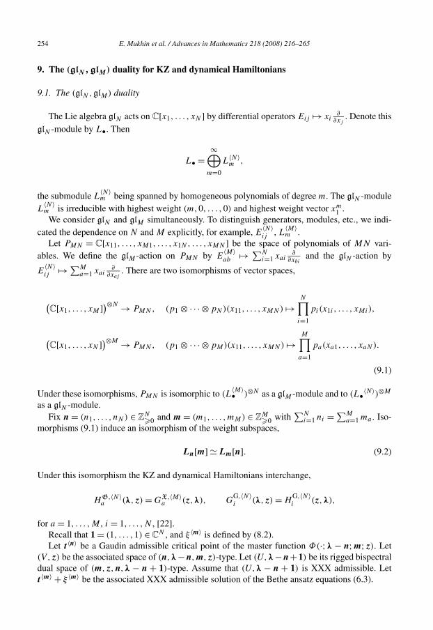
254 E. Mukhin et al. / Advances in Mathematics 218 (2008) 216–265
9. The (glN,glM) duality for KZ and dynamical Hamiltonians
9.1. The (glN,glM) duality
The Lie algebra glN acts on C[x1, . . . , xN ] by differential operators Eij → xi∂
∂xj. Denote this
glN -module by L•. Then
L• =∞⊕
m=0
L〈N〉m ,
the submodule L〈N〉m being spanned by homogeneous polynomials of degree m. The glN -module
L〈N〉m is irreducible with highest weight (m,0, . . . ,0) and highest weight vector xm
1 .We consider glN and glM simultaneously. To distinguish generators, modules, etc., we indi-
cated the dependence on N and M explicitly, for example, E〈N〉ij , L
〈M〉m .
Let PMN = C[x11, . . . , xM1, . . . , x1N, . . . , xMN ] be the space of polynomials of MN vari-ables. We define the glM -action on PMN by E
〈M〉ab → ∑N
i=1 xai∂
∂xbiand the glN -action by
E〈N〉ij → ∑M
a=1 xai∂
∂xaj. There are two isomorphisms of vector spaces,
(C[x1, . . . , xM ])⊗N → PMN, (p1 ⊗ · · · ⊗ pN)(x11, . . . , xMN) →
N∏i=1
pi(x1i , . . . , xMi),
(C[x1, . . . , xN ])⊗M → PMN, (p1 ⊗ · · · ⊗ pM)(x11, . . . , xMN) →
M∏a=1
pa(xa1, . . . , xaN).
(9.1)
Under these isomorphisms, PMN is isomorphic to (L〈M〉• )⊗N as a glM -module and to (L•〈N〉)⊗M
as a glN -module.Fix n = (n1, . . . , nN) ∈ ZN
�0 and m = (m1, . . . ,mM) ∈ ZM�0 with
∑Ni=1 ni = ∑M
a=1 ma . Iso-morphisms (9.1) induce an isomorphism of the weight subspaces,
Ln[m] � Lm[n]. (9.2)
Under this isomorphism the KZ and dynamical Hamiltonians interchange,
HG,〈N〉a (λ,z) = GX,〈M〉
a (z,λ), GG,〈N〉i (λ,z) = H
G,〈N〉i (z,λ),
for a = 1, . . . ,M , i = 1, . . . ,N , [22].Recall that 1 = (1, . . . ,1) ∈ CN , and ξ 〈m〉 is defined by (8.2).Let t 〈n〉 be a Gaudin admissible critical point of the master function Φ(·;λ − n;m;z). Let
(V ,z) be the associated space of (n,λ−n,m,z)-type. Let (U,λ−n+1) be its rigged bispectraldual space of (m,z,n,λ − n + 1)-type. Assume that (U,λ − n + 1) is XXX admissible. Lett 〈m〉 + ξ 〈m〉 be the associated XXX admissible solution of the Bethe ansatz equations (6.3).
E. Mukhin et al. / Advances in Mathematics 218 (2008) 216–265 255
Conjecture 9.1. The corresponding Bethe vectors ωG(t 〈n〉,z) ∈ Lm[n] and ωX(t 〈m〉,λ) ∈Ln[m] are proportional under the duality isomorphism (9.2).
We prove this conjecture for N = M = 2 in Section 10.4, see also [13].
10. The case of N = M = 2
10.1. The (gl2,gl2) duality
Let n = (n1, n2) and m = (m1,m2) be two vectors of nonnegative integers such that n1 +n2 =m1 + m2.
Fix λ = (λ1, λ2) and z = (z1, z2) each with distinct coordinates.For m ∈ Z�0, let Lm be the irreducible gl2-module with highest weight (m,0) and highest
weight vector vm. The vectors Ei21vm, i = 0, . . . ,m, form a basis in Lm.
Set
α = max(0, n2 − m1), β = min(m2, n2).
The vectors
En2−i21 vm1
(n2 − i)! ⊗ Ei21vm2
i! , α � i � β,
form a basis in Lm[n] = (Lm1 ⊗ Lm2)[n1, n2]. The vectors
Em2−i21 vn1
(m2 − i)! ⊗ Ei21vn2
i! , α � i � β,
form a basis in Ln[m] = (Ln1 ⊗ Ln2)[m1,m2]. Isomorphism (9.2) identifies the vectors with thesame index i.
We consider the Gaudin Hamiltonians on Lm[n] and the XXX Hamiltonians on Ln[m].Let Bi,j (t) be the series defined in Section 8.2. Consider the map
b(λ) : (Lm1 ⊗ Lm2)[n1, n2] → (Lm1 ⊗ Lm2)[n2, n1] (10.1)
defined by the formula
En2−i21 vm1
(n2 − i)! ⊗ Ei21vm2
i! → B21(λ1 − λ2)E
m1−n2+i21 vm1
(m1 − n2 + i)! ⊗ Em2−i21 vm2
(m2 − i)! .
For a generic λ this map is an isomorphism.By [21], the map b(λ) commutes with the Gaudin Hamiltonians in the following sense:
b(λ)HGa (λ1, λ2,z) = HG
a (λ2, λ1,z)b(λ),
b(λ)GGi (λ1, λ2,z) = GG
i (λ2, λ1,z)b(λ)
for a, i = 1,2.
256 E. Mukhin et al. / Advances in Mathematics 218 (2008) 216–265
The map
Em2−i21 vn1
(m2 − i)! ⊗ Ei21vn2
i! → En1−m2+i21 vn1
(n1 − m2 + i)! ⊗ En2−i21 vn2
(n2 − i)! (10.2)
defines the Weyl isomorphism
s : (Ln1 ⊗ Ln2)[m1,m2] → (Ln1 ⊗ Ln2)[m2,m1]. (10.3)
The Weyl isomorphism commutes with the XXX Hamiltonians,
sHXi (z,λ) = HX
i (z,λ)s,
sGXa (z,λ) = GX
a (z,λ)s
for i, a = 1,2.
10.2. The Gaudin universal rational function and the fundamental differential equation
Let n = (n1, n2) and m = (m1,m2) be two vectors of nonnegative integers such that n1 +n2 =m1 + m2.
Fix λ = (λ1, λ2) and z = (z1, z2) each with distinct coordinates. The Gaudin universal ratio-nal Lm[n]-valued function is the function
ω(t1, . . . , tn2) =∑
i
Ci
En2−i21 vm1
(n2 − i)! ⊗ Ei21vm2
i! ,
where
Ci(t1, . . . , tn2) = Symn2
[n2−i∏j=1
1
tj − z1
i∏j=1
1
tn2+j−i − z2
](10.4)
and Symn f (t1, . . . , tn) = ∑σ∈Σn
f (tσ (1), . . . , tσ (n)), see [9].
The Gaudin universal rational function is symmetric with respect to the group Σn2 of permu-tations of variables t1, . . . , tn2 . The Σn2 -orbit of a point t 〈n〉 = (t1, . . . , tn2) is represented by thepolynomial p(x) = (x − t1) · · · (x − tn2).
The polynomials (x−z1)n2−i (x−z2)
i , i = 0, . . . , n2, form a basis in the space of polynomialsin x of degree not greater than n2.
Lemma 10.1. Let p(x) = (x − t1) · · · (x − tn2) be a polynomial. Let the numbers C0, . . . ,Cn2 begiven by formula (10.4). Then
(z1 − z2)n2p(x)
p(z1)p(z2)=
n2∑i=0
(−1)iCi
(x − z1)n2−i
(n2 − i)!(x − z2)
i
i! .

E. Mukhin et al. / Advances in Mathematics 218 (2008) 216–265 257
The proof is straightforward.Let V = 〈xλ1p1(x), xλ2p2(x)〉. Let (V ,z) be a space of (n,λ,m,z)-type. The rigged funda-
mental differential operator of (V ,z) has the form
D = (x − z1)(x − z2)(x∂x − λ1 − n1)(x∂x − λ2)
+ φ11x(x − z1)(x∂x − λ1 − n1) + φ12z2(x − z1)(x∂x − λ2)
+ φ21x(x − z2)(x∂x − λ1 − n1) + φ22z1(x − z2)(x∂x − λ2),
where φij are suitable numbers such that
φ21 + φ22 = −m1, φ11 + φ12 = −m2,
φ22 + φ12 = −n1, φ21 + φ11 = −n2. (10.5)
The operator D can be written also in the form
D = (x − z1)(x − z2)(x∂x − λ1 − n1)(x∂x − λ2 − n2)
+ ψ11x(x − z1)(x∂x − λ1) + ψ12z2(x − z1)(x∂x − λ2 − n2)
+ ψ21x(x − z2)(x∂x − λ1) + ψ22z1(x − z2)(x∂x − λ2 − n2),
where ψij are such that
ψ21 + ψ22 = −m1, ψ11 + ψ12 = −m2,
ψ22 + ψ12 = −n1, ψ21 + ψ11 = −n2,
and ψ11(λ1 − λ2 − n2) = φ11(λ1 − λ2 + n1) + m2n2.Equation Df = 0 has a solution
f (x) = xλ2p2(x) = xλ2
n2∑i=0
ci
(x − z1)n2−i
(n2 − i)!(x − z2)
i
i! .
Due to conditions (10.5), the expression x−λ2Df (x) is a polynomial of degree at most n2 + 1vanishing at x = 0. Expanding this polynomial as a linear combination of the polynomialsx(x − z1)
n2−i (x − z2)i , i = 0, . . . , n2, we obtain that the equation Df = 0 is equivalent to the
following relations for the coefficients c0, . . . , cn2 :
z1i(m1 − n2 + i)ci−1 + z2(m2 − i)(n2 − i)ci+1
+ ((z1 + z2)i
2 + (z2m1 − z1m2 − 2z2n2 − (λ1 − λ2)(z1 − z2)
)i
− (λ1 − λ2 + n1)(z1 − z2)φ11 + z2m2n2)ci = 0, (10.6)
i = 0, . . . , n2. Notice that values i = 0, n2 − m1,m2, n2 are the values of i for which Eq. (10.6)does not contain ci−1 or ci+1.

258 E. Mukhin et al. / Advances in Mathematics 218 (2008) 216–265
Lemma 10.2. Eqs. (10.6) with i such that α � i � β form a closed system of equations withrespect to cj such that α � j � β .
The proof is straightforward.
Eqs. (10.6) have a symmetry. Namely, (10.6) does not change if we replace the parametersλ1, λ2, n1, n2, φ11, i by λ2, λ1, n2, n1,ψ12,m2 − i, respectively, and after that replace the un-knowns cj by (z1/z2)
j cm2−j .
10.3. The XXX universal rational function and the fundamental difference equation
Let n = (n1, n2) and m = (m1,m2) be two vectors of nonnegative integers such that n1 +n2 =m1 + m2.
Fix λ = (λ1, λ2) and z = (z1, z2) each with distinct coordinates. The XXX universal rationalLn[m]-valued function is the function
ω(s1, . . . , sm2 ,λ) =∑
i
Ci
Em2−i21 vn1
(m2 − i)! ⊗ Ei21vn2
i! ,
where
Ci(s1, . . . , sm2 ,λ) = Symm2
[m2−i∏a=1
1
sa − λ1 + n1
m2∏b=m2−i+1
sb − λ1
(sb − λ1 + n1)(sb − λ2 + n2)
×m2−i∏a=1
m2∏b=m2−i+1
sa − sb − 1
sa − sb
], (10.7)
see [8,20].The XXX universal rational function is symmetric with respect to the group Σm2 of permuta-
tions of variables s1, . . . , sm2 . The Σm2 -orbit of a point s〈n〉 = (s1, . . . , sm2) is represented by thepolynomial q(u) = (u − s1) · · · (u − sm2).
The polynomials∏m2−i−1
j=0 (u − λ1 + n1 − j)∏i−1
j=0(u − λ2 + j), i = 0, . . . ,m2, form a basisin the space of polynomials in x of degree not greater than m2.
Lemma 10.3. Let q(u) = (u − s1) · · · (u − sm2) be a polynomial. Let the numbers C0, . . . ,Cm2
be given by formula (10.7). Then
q(u)
q(λ1 − n1)q(λ2 − n2)
m2−1∏j=0
(λ1 − λ2 + n2 − j)
=m2∑i=0
(−1)iCi(s1, . . . , sm2 ,λ)
(m2 − i)!i!m2−i−1∏
j=0
(u − λ1 + j)
i−1∏j=0
(u − λ2 + n2 − j).
The proof is straightforward.

E. Mukhin et al. / Advances in Mathematics 218 (2008) 216–265 259
Let U = 〈zu1q1(u), zu
2q2(u)〉. Let (U,λ) be a space of (m,z,n,λ)-type. The rigged fundamen-tal difference operator of (U,λ) has the form
D = (u − λ1 − n1 + 1)(u − λ2 + 1)(τ − z1)(τ − z2)
+ ϕ11(u − λ1 − n1 + 1)τ (τ − z1) + ϕ12(u − λ2 + 1)z2(τ − z1)
+ ϕ21(u − λ1 − n1 + 1)τ (τ − z2) + ϕ22(u − λ2 + 1)z1(τ − z2),
where ϕij are suitable numbers such that
ϕ21 + ϕ22 = −m1, ϕ11 + ϕ12 = −m2,
ϕ22 + ϕ12 = −n1, ϕ21 + ϕ11 = −n2. (10.8)
Equation Df = 0 has a solution
f = zu2q2(u) = zu
2
m2∑i=1
ci
(m2 − i)!i!m2−i−1∏
j=0
(u − λ1 − n1 + j)
i−1∏j=0
(u − λ2 − j).
Due to conditions (10.8), the expression z−u2 Df (u) is a polynomial of degree at most m2. Ex-
panding this polynomial as a linear combination of the polynomials
m2−i−1∏j=0
(u − λ1 − n1 + j + 1)
i−1∏j=0
(u − λ2 − j + 1), i = 0, . . . ,m2,
we obtain that the equation Df = 0 is equivalent to the following relations for the coefficientsc0, . . . , cm2 :
z1i(m1 − n2 + i)ci−1 + z2(m2 − i)(n2 − i)ci+1
+ ((z1 + z2)i
2 + (z2m1 − z1m2 − 2z2n2 − (λ1 − λ2)(z1 − z2)
)i
− (λ1 − λ2 + n1)(z1 − z2)ϕ11 + z2m2n2)ci = 0, (10.9)
i = 0, . . . ,m2. Notice that values i = 0, n2 − m1,m2, n2 are the values of i for which Eq. (10.6)does not contain ci−1 or ci+1.
Lemma 10.4. Eqs. (10.9) with i such that α � i � β form a closed system of equations withrespect to cj such that α � j � β .
The proof is straightforward.Eqs. (10.9) have a symmetry. Namely, (10.9) does not change if we replace the parameters
z1, z2,m1,m2, ϕ11, i by z2, z1,m2,m1, ϕ21, n2 − i, respectively, and after that replace the un-knowns cj by cn2−j . Another symmetry of (10.9) is that the equations do not change if wereplace λ1, λ2 by λ1 + 1, λ2 + 1.
The pair of Eqs. (10.6) and (10.9) have a symmetry. Namely, Eq. (10.6) turns into Eq. (10.9)if we replace the parameter φ11 there by ϕ11.

260 E. Mukhin et al. / Advances in Mathematics 218 (2008) 216–265
10.4. Proof of Conjecture 9.1 for N = M = 2
The symmetries of Eqs. (10.6) and (10.9) imply the following theorem.
Theorem 10.5. Let V = 〈xλ1p1(x), xla2p2(x)〉 and U = 〈zu1q1(u), zu
2q2(u)〉. Let (V ,z) be aspace of (n,λ,m,z)-type and (U,λ + 1) the rigged bispectral dual space of (m,z,n,λ + 1)-type, where 1 = (1,1). Write
p2(x) =n2∑i=0
ci(λ)(x − z1)
n2−i
(n2 − i)!(x − z2)
i
i! ,
p1(x) =n1∑i=0
di(λ)(x − z1)
n1−i
(n1 − i)!(x − z2)
i
i! ,
q2(u) =m2∑i=1
ei(λ + 1)
(m2 − i)!i!m2−i−1∏
j=0
(u − λ1 − 1 − n1 + j)
i−1∏j=0
(u − λ2 − 1 − j),
q1(u) =m1∑i=1
fi(λ + 1)
(m1 − i)!i!m1−i−1∏
j=0
(u − λ1 − 1 − n1 + j)
i−1∏j=0
(u − λ2 − 1 − j).
Then there exist nonzero numbers A(λ),B(λ),C(λ) such that
ci(λ) = A(λ)dm2−i (λ)(z1/z2)i = B(λ)ei(λ + 1) = C(λ)fn2−i (λ + 1)
for all i, α � i � β .
Theorems 10.5 and 8.1 yield the next statement.
Corollary 10.6. The Bethe vectors
β∑i=α
ci(λ + n)E
n2−i21 vm1
(n2 − i)! ⊗ Ei21vm2
i! ,
β∑i=α
di(λ + n)E
n1−i21 vm1
(n1 − i)! ⊗ Ei21vm2
i! ,
β∑i=α
ei(λ + n)E
m2−i21 vn1
(m2 − i)! ⊗ Ei21vn2
i! ,
β∑i=α
fi(λ + n)E
m1−i21 vn1
(m1 − i)! ⊗ Ei21vn2
i!
are identified up to proportionality by isomorphisms (10.1) and (9.2).
The fact that the first and second Bethe vectors are identified by isomorphism (10.1) is provedalso in [16] in a different way.

E. Mukhin et al. / Advances in Mathematics 218 (2008) 216–265 261
10.5. Correspondence of solutions of the Bethe ansatz equations for N = M = 2
Consider the following four systems of the Bethe ansatz equations:
λ1 − λ2 − 1
ti+
2∑a=1
ma
ti − za
−n2∑
j=1,j �=i
2
ti − tj= 0, i = 1, . . . , n2, (10.10)
λ1 − λ2 − 1
ti+
2∑a=1
ma
ti − za
−n1∑
j=1,j �=i
2
ti − tj= 0, i = 1, . . . , n1, (10.11)
2∏i=1
ta − λi − 1
ta − λi − 1 − ni
m2∏b,b �=a
ta − tb − 1
tb − tb + 1= z2
z1, a = 1, . . . ,m2, (10.12)
2∏i=1
ta − λi − 1
ta − λi − 1 − ni
m1∏b,b �=a
ta − tb − 1
tb − tb + 1= z2
z1, a = 1, . . . ,m1. (10.13)
The first two systems are of the Gaudin type and the last two systems are of the XXX type, see(6.2) and (6.3).
Set d = dim(Lm1 ⊗ Lm2)[n1, n2] = dim(Lm1 ⊗ Lm2)[n2, n1] = dim(Ln1 ⊗ Ln2)[m1,m2] =dim(Ln1 ⊗ Ln2)[m2,m1]. By [17] for generic λ and z each of the first two systems has exactly d
orbits of Gaudin admissible solutions. By [17] for generic λ and z each of the last two systemshas exactly d orbits of XXX admissible solutions.
Theorem 10.7. Let λ and z be generic. Let (t1, . . . , tn2) be a Gaudin admissible solution of thesystem (10.10). Let (V ,z) = 〈xλ1p1(x), xλ2p2(x)〉 be the space of (λ,z,n,m)-type associatedwith the orbit of the critical point. Let (U,λ + 1) = 〈zu
1q1(u), zu2q2(u)〉, where 1 = (1,1) , be the
rigged bispectral dual space to (V ,z). Then the polynomial p1 represents the orbit of a Gaudinadmissible solution of the system (10.11), the polynomial q2 represents the orbit of an XXXadmissible solution of the system (10.12), and the polynomial q1 represents the orbit of an XXXadmissible solution of the system (10.13).
11. Baker–Akhiezer functions and bispectral correspondence
In this section we indicate a connection of our integral transforms of Section 4 with the bis-pectral theory, see [24,7,6,2,1].
11.1. Grassmannian of Gaudin admissible nondegenerate spaces
For λ ∈ C, we call a vector subspace Xλ ⊂ C[u] Gaudin admissible at λ if there existsm ∈ Z�0 such that
(u − λ)(u − λ − 1) · · · (u − λ − m + 1)C[u] ⊂ Xλ
and there exists f ∈ Xλ such that f (λ) �= 0. We call a vector subspace X ⊂ C[u] Gaudin admis-sible if

262 E. Mukhin et al. / Advances in Mathematics 218 (2008) 216–265
X =n⋂
i=1
Xλi
where n is a natural number, λ1, . . . , λn ∈ C are such that λi −λj /∈ Z if i �= j , and for any i, Xλi
is Gaudin admissible at λi .Each Xλi
can be defined by a finite set of linear equations. Namely, there exist a positive inte-ger Ni , a sequence of integers 0 < ni1 < · · · < niNi
and complex numbers ci,j,a , a = 0, . . . , nij ,such that ci,j,nij
�= 0 for all i, j . Then the space Xλiconsists of all polynomials r ∈ C[u] satisfy-
ing the equations
nij∑a=0
ci,j,ar(λi + a) = 0 for j = 1, . . . ,Ni. (11.1)
For a Gaudin admissible subspace X, define the complex vector space V as the space spannedby functions xλi pij (x), i = 1, . . . , n, j = 1, . . . ,Ni , where pij (x) = ∑nij
a=0 ci,j,axa . The space V
is a space of quasi-polynomials of the type considered in Section 2.1.On the other hand, having a space V of quasi-polynomials, as in Section 2.1, we can recover
a Gaudin admissible subspace X ⊂ C[u] by formula (11.1).We say that the space X is nondegenerate if the corresponding space V is nondegenerate in
the sense of Section 2.1.We denote the set of all Gaudin admissible nondegenerate subspaces by GrG and call it the
Grassmannian of the Gaudin admissible nondegenerate subspaces.Let X ⊂ C[u] be a Gaudin admissible subspace and V the associated space of quasi-
polynomials in x. Define the algebra AX = {p ∈ C[u] | p(u)X ⊂ X}. An equivalent definition isAX = {p ∈ C[u] | p(x∂x)V ⊂ V }.
Let DV be the monic fundamental differential operator of V . The function
ΨX(x,u) =n∏
i=1
Ni∏j=1
x
u − λi − nij
DV xu
will be called the stationary Baker–Akhiezer function of the Gaudin admissible space X. In-troduce the rational function ψX(x,u) by the formula ΨX(x,u) = ψX(x,u)xu. The functionψX(x,u) expands as a power series in x−1, u−1 of the form
ψX(x,u) = 1 +∞∑
i,j=1
cij x−iu−j .
It is easy to see that for every p ∈ AX , there exists a linear differential operator Lp(x, ∂x) withrational coefficients such that Lp(x, ∂x)DV = DV p(x∂x). As a corollary, we conclude that
Lp(x, ∂x)ΨX(x,u) = p(u)ΨX(x,u).
For p1,p2 ∈ A, the corresponding operators Lp (x, ∂x) and Lp (x, ∂x) commute.
1 2
E. Mukhin et al. / Advances in Mathematics 218 (2008) 216–265 263
11.2. Grassmannian of XXX admissible nondegenerate spaces
Let z ∈ C∗ be a nonzero complex number with fixed argument. We call a vector subspaceYz ⊂ C[x] XXX admissible at z if there exists n ∈ Z�0 such that (x − z)nC[x] ⊂ Yz and thereexists f ∈ Yz such that f (z) �= 0. We call a vector subspace Y ⊂ C[x] XXX admissible if
Y =m⋂
a=1
Yza
where m is a natural number, z1, . . . , zm ∈ C∗ are distinct numbers and for any a, the space Yza
is XXX admissible at za .Each Yza can be defined by a finite set of linear equations. Namely, there exist a posi-
tive integer Ma , a sequence of integers 0 < ma1 < · · · < maMa and complex numbers da,b,i ,i = 0, . . . ,mab , such that da,b,mab
�= 0 for all a, b. Then the space Yza consists of all polynomialsr ∈ C[x] satisfying the equations
mab∑i=0
da,b,i (x∂x)ir(za) = 0 for b = 1, . . . ,Ma. (11.2)
For an XXX admissible subspace Y define the complex vector space U as the space spannedby functions zu
aqab(u), a = 1, . . . ,m, b = 1, . . . ,Ma , where
zuaqab(u) = zu
a
mab∑i=0
da,b,iui .
The space U is a space of quasi-exponentials in u of the type considered in Section 3.1.On the other hand, having a space U of quasi-exponentials, as in Section 3.1, we can recover
an XXX admissible subspace Y ⊂ C[x] by formula (11.2).We say that Y is nondegenerate if the corresponding U is nondegenerate in the sense of
Section 3.6.We denote the set of all XXX admissible nondegenerate subspaces by GrX and call it the
Grassmannian of the XXX admissible nondegenerate subspaces.Let Y ⊂ C[x] be an XXX admissible subspace and U the associated space of quasi-
exponentials. Define the algebra AY = {p ∈ C[x] | p(x)W ⊂ W }. An equivalent definition isAY = {p ∈ C[x] | p(τu)U ⊂ U}.
Let DU be the monic fundamental difference operator of U . The function
ΦY (u, x) =m∏
a=1
(x − za)−MaDUxu
will be called the stationary Baker–Akhiezer function of the XXX admissible space Y . Introducethe rational function φY (u, x) by the formula ΦY (u, x) = φY (u, x)xu. The function φY (u, x)
expands as a power series in u−1, x−1 of the form
φY (u, x) = 1 +∞∑
ciju−ix−j .
i,j=1

264 E. Mukhin et al. / Advances in Mathematics 218 (2008) 216–265
It is easy to see that for every p ∈ AY , there exists a linear difference operator Lp(u, τu) withrational coefficients such that Lp(u, τu)DV = DV p(τu). As a corollary, we conclude that
Lp(u, τu)ΦY (u, x) = p(x)ΦY (u, x).
For p1,p2 ∈ A, the corresponding operators Lp1(u, τu) and Lp2(u, τu) commute.
11.3. Bispectral correspondence
In terms of the Baker–Akhiezer functions, we introduce a bispectral correspondence betweenpoints of the Grassmannian of Gaudin admissible nondegenerate subspaces and points of theGrassmannian of XXX admissible nondegenerate subspaces. We say that a Gaudin admissiblenondegenerate space X corresponds to an XXX admissible nondegenerate space Y if ΨX(x,u) =ΦY (u, x). This correspondence is an analog of Wilson’s bispectral correspondence in [24], seealso the papers [7,6,2,1].
Theorem 11.1. Let V be a nondegenerate space of quasi-polynomials and let U be the non-degenerate space of quasi-exponentials which are bispectral dual with respect to the integraltransforms of Section 4. Then the corresponding admissible spaces X ∈ GrG and Y ∈ GrX arebispectral correspondent.
Acknowledgments
Authors thank Yu. Berest and O. Chalykh for discussions and for providing the authors withmanuscripts [2,1] after the present work had been written.
References
[1] Yu. Berest, O. Chalykh, Calogero–Moser correspondence: trigonometric case, preprint, 2004, 15 pp.[2] Yu. Berest, O. Chalykh, Quasi-exponentials, quasi-polynomials and Calogero–Moser spaces, preprint, 2007, 6 pp.[3] I.V. Cherednik, Generalized braid groups and local r-matrix systems, Dokl. Akad. Nauk SSSR 307 (1) (1989)
49–53.[4] I.B. Frenkel, N.Yu. Reshetikhin, Quantum affine algebras and holonomic difference equations, Comm. Math.
Phys. 146 (1992) 1–60.[5] W. Fulton, Intersection Theory, Springer-Verlag, 1984.[6] L. Haine, KP Trigonometric Solitons and an Adelic Flag Manifold, SIGMA 3 015 (2007) 1–15.[7] L. Haine, P. Iliev, Commutative rings of difference operators and an adelic flag manifold, Int. Math. Res. Not. 6
(2000) 281–323.[8] V. Korepin, N. Bogoliubov, A. Izergin, Quantum Inverse Scattering Method and Correlation Functions, Cambridge
University Press, Cambridge, 1993.[9] Y. Markov, A. Varchenko, Hypergeometric solutions of trigonometric KZ equations satisfy dynamical difference
equations, Adv. Math. 166 (1) (2002) 100–147.[10] E. Mukhin, V. Tarasov, A. Varchenko, Bispectral and (glN ,glM) Dualities, Functional Analysis and Other Mathe-
matics 1 (1) (2006) 55–80.[11] E. Mukhin, V. Tarasov, A. Varchenko, The B. and M. Shapiro conjecture in real algebraic geometry and the Bethe
ansatz, Ann. of Math., in press, http://annals.math.princeton.edu/issues/2007/AnnalsAcceptedPapers2007.pdf.[12] E. Mukhin, V. Tarasov, A. Varchenko, Bethe eigenvectors of higher transfer matrices, J. Stat. Mech. Theory Exp. 8
(2006), P08002, 44 pp. (electronic).[13] E. Mukhin, V. Tarasov, A. Varchenko, A generalization of the Capelli identity, math.QA/0610799, 14 pp.; Al-
gebra, Arithmetic and Geometry—Manin Festschrift, in press, http://www.math.nyu.edu/~tschinke/.manin/manin-index.html.

E. Mukhin et al. / Advances in Mathematics 218 (2008) 216–265 265
[14] E. Mukhin, A. Varchenko, Solutions to the XXX type Bethe ansatz equations and flag varieties, Cent. Eur. J.Math. 1 (2) (2003) 238–271.
[15] E. Mukhin, A. Varchenko, Critical points of master functions and flag varieties, Commun. Contemp. Math. 6 (1)(2004) 111–163.
[16] E. Mukhin, A. Varchenko, Multiple orthogonal polynomials and a counterexample to the Gaudin Bethe Ansatzconjecture, Trans. Amer. Math. Soc. 359 (11) (2007) 5383–5418.
[17] E. Mukhin, A. Varchenko, Spaces of quasi-polynomials and Bethe Ansatz, math.QA/0604048, 29 pp.[18] N. Reshetikhin, A. Varchenko, Quasiclassical asymptotics of solutions to the KZ equations, in: Geometry, Topology,
& Physics, in: Conf. Proc. Lecture Notes Geom. Topology, vol. IV, Internat. Press, Cambridge, MA, 1995, pp. 293–322.
[19] V. Tarasov, A. Varchenko, Jackson integral representations for solutions of the Knizhnik–Zamolodchikov quantumequation, Algebra i Analiz 6 (2) (1994) 90–137 (in Russian), translation in St. Petersburg Math. J. 6 (2) (1995)275–313.
[20] V. Tarasov, A. Varchenko, Asymptotic solutions to the quantized Knizhnik–Zamolodchikov equation and Bethe vec-tors, in: Mathematics in St. Petersburg, in: Amer. Math. Soc. Transl. Ser. 2, vol. 174, Amer. Math. Soc., Providence,RI, 1996, pp. 235–273.
[21] V. Tarasov, A. Varchenko, Difference equations compatible with trigonometric KZ differential equations, Int. Math.Res. Not. 15 (2000) 801–829.
[22] V. Tarasov, A. Varchenko, Duality for Knizhnik–Zamolodchikov and dynamical equations, Acta Appl. Math.73 (1–2) (2002) 141–154.
[23] V. Tarasov, A. Varchenko, Dynamical differential equations compatible with rational qKZ equations, Lett. Math.Phys. 71 (2) (2005) 101–108.
[24] G. Wilson, Collisions of Calogero–Moser particles and an adelic Grassmannian, Invent. Math. 133 (1998) 1–41.