BIS Working Papers · Hyun Song Shin Monetary and Economic Department January 2018 JEL...

BIS Working PapersNo 695

The dollar exchange rate as a global risk factor: evidence from investment by Stefan Avdjiev, Valentina Bruno, Catherine Koch and Hyun Song Shin

Monetary and Economic Department

January 2018

JEL classification: F31, F32, F34, F41

Keywords: financial channel, exchange rates, cross-border bank lending, real investment

BIS Working Papers are written by members of the Monetary and Economic Department of the Bank for International Settlements, and from time to time by other economists, and are published by the Bank. The papers are on subjects of topical interest and are technical in character. The views expressed in them are those of their authors and not necessarily the views of the BIS.

This publication is available on the BIS website (www.bis.org).

© Bank for International Settlements 2018. All rights reserved. Brief excerpts may be reproduced or translated provided the source is stated.

ISSN 1020-0959 (print) ISSN 1682-7678 (online)

1

The dollar exchange rate as a global risk factor: evidence from investment1

Stefan Avdjiev (BIS)

Valentina Bruno (American University)

Catherine Koch (BIS)

Hyun Song Shin (BIS)

Paper prepared for the IMF 18th Jacques Polak Annual Research Conference

Abstract

Exchange rate fluctuations influence economic activity not only via the standard trade channel, but also through a financial channel, which operates through the impact of exchange rate fluctuations on borrowers’ balance sheets and lenders’ risk-taking capacity. This paper explores the “triangular” relationship between (i) the strength of the US dollar, (ii) cross-border bank flows and (iii) real investment. We conduct two sets of empirical exercises - a macro (country-level) study and a micro (firm-level) study. We find that a stronger dollar is associated with lower growth in dollar-denominated cross-border bank flows and lower real investment in emerging market economies. An important policy implication of our findings is that a stronger dollar has real macroeconomic effects that go in the opposite direction to the standard trade channel.

1 We thank Signe Krogstrup, Amal Mattoo, Linda Tesar, two anonymous referees, participants at the IMF 18th Jacques Polak Annual Research Conference and seminar participants at the Federal Reserve Board for valuable comments and suggestions. Bat-el Berger and Zuzana Filková provided excellent research assistance. We also thank Stijn Claessens, Hui Tong, and Shang-Jin Wei for sharing their data series on financial dependence. The views expressed are those of the authors and not necessarily those of the Bank for International Settlements.

2

1. Introduction

Exchange rate fluctuations influence economic activity through both real and financial channels. The

conventional trade channel with effects on the real economy operates through net exports. This channel

is well-known and standard in open-economy macro models. By contrast, the financial channel operates

through exchange rate fluctuations which trigger valuation changes, balance-sheet adjustments and shifts

in risk-taking, both in financial and real assets, with impact on the real economy. Although the financial

channel of exchange rates has historically been less prominent than the net exports channel, it has

become more important with the greater integration of the global financial system in recent years.

Crucially, the financial channel of exchange rate fluctuations often operates in the opposite direction

relative to the net exports channel. Specifically, under the net exports channel, it is when the domestic

currency depreciates that real economic activity picks up. By contrast, the financial channel operates

through the liabilities side of the balance sheet of domestic borrowers, so that it is when the domestic

currency appreciates that balance sheets strengthen and economic activity picks up.

The key empirical regularity at the heart of the financial channel of exchange rates is the empirical

association between the depreciation of an international funding currency and the greater borrowing in

that currency by non-residents. In the specific case of the US dollar, the empirical regularity is that when

the dollar depreciates against the currency of a given country, the residents of that country tend to borrow

more in US dollars.

This empirical regularity has several drivers, both on the demand for dollar credit on the part of

borrowers and on the supply of dollar credit by lenders. In terms of the demand for dollar credit, a

borrower who had borrowed in dollars to finance domestic real estate assets would see a strengthening

of their balance sheet due to the depreciation of the dollar. More commonly, an exporting firm with dollar

receivables or an asset manager with dollar-denominated assets – but with domestic currency obligations

– would hedge currency risk more aggressively when the dollar is expected to depreciate more. Incurring

dollar liabilities, or an equivalent transaction off balance sheet, would be the way to hedge currency risk

in such instances.

The link between dollar depreciation and greater borrowing in dollars by non-residents may also

operate through the supply of dollar credit, and has been dubbed the “risk-taking channel” by Bruno and

Shin (2015b). When there is the potential for valuation mismatches on borrowers’ balance sheets arising

from exchange rate fluctuations, a weaker dollar flatters the balance sheet of dollar borrowers, whose

3

liabilities fall relative to assets. From the standpoint of creditors, the stronger credit position of the

borrowers reduces tail risk in the credit portfolio and creates spare capacity for additional credit extension

even with a fixed exposure limit as given by a value-at-risk (VaR) constraint or an economic capital (EC)

constraint.

The financial channel of exchange rate fluctuations has both a price and a quantity dimension. The

price dimension has been addressed by Hofmann et al (2016) and Avdjiev et al (2017). Hofmann et al

(2016) use data on sovereign bond spreads to show that a currency appreciation is associated with greater

risk-taking by both borrowers and lenders. There is also rapidly mounting empirical evidence for the

existence of the quantity dimension of the financial channel of exchange rate fluctuations. Avdjiev et al

(2017) have demonstrated that an appreciation in the US dollar is associated with contractions in cross-

border bank lending denominated in US dollars. In addition, Kearns and Patel (2016) have found evidence

that the financial channel partly offsets the trade channel for emerging market economies (EMEs) and

that investment is found to be particularly sensitive to the financial channel.

In this paper, we build on the literature above by exploring the “triangular” relationship between (i)

the strength of the US dollar, (ii) cross-border bank flows and (iii) real investment. More specifically, we

examine the triangular relationship through two sets of empirical exercises – a macro (country-level)

study, and a micro (firm-level) study. In the first one, we examine evidence from structural panel vector

autoregressions (SPVARs) using country-level data on real investment, cross-border bank credit, the

strength of the US dollar, US monetary policy and global uncertainty. In the second study, we estimate

the relationship between corporate capital expenditure (CAPEX) and the strength of the US dollar (while

controlling for a number of additional factors) in a firm-level panel setup.

In principle, there are three concepts of exchange rates that could potentially be relevant. First, in

the classic Mundell-Fleming paradigm, the trade-weighted exchange rate of a given country affects

economic activity in that country through its impact on net exports. Second, the bilateral exchange rate

of a country’s currency vis-à-vis the US dollar operates through both net exports via its impact on import

prices and quantities (as highlighted by the “dominant currency paradigm” literature) and credit demand

from local borrowers via its impact on the net worth of borrowers with currency mismatches on their

balance sheets (as emphasised by the EME crisis literature). Third, the broad US dollar index affects the

credit risk in a diversified portfolio of US dollar-denominated loans of borrowers with currency

mismatches and determines the tail risk in a diversified global portfolio of dollar-denominated loans of

global banks. As a consequence, it has an impact on the supply of credit by global banks through the value-

4

at-risk (VaR) constraint (Bruno and Shin, 2015a and 2015b; Avdjiev et al, 2016). Which of the above three

exchange rates is most relevant for real investment is the subject of our empirical investigation.

We find that a stronger US dollar is associated with lower dollar-denominated cross-border bank

flows and lower real investment in EMEs. Our empirical investigation establishes four findings. First, in

line with the predictions of Bruno and Shin (2015b), we find a negative relationship between the strength

of the US dollar and cross-border bank lending denominated in US dollars, both for the bilateral dollar

exchange rate and the broad dollar index. Second, increases in US dollar-denominated cross-border bank

credit to a given EME are associated with greater real investment in that EME. Third, the combination of

the first two relationships results in the most important link that we discover – an appreciation of the US

dollar leads to a decline in real investment. Finally, we find that the broad dollar index is the most relevant

exchange rate for real investment, in line with previous studies that have found that dollar lending by

global banks fluctuates with the broad dollar index and highlight the prevalence of the credit supply

mechanism (Avdjiev et al, 2016; Avdjiev et al, 2017).

Our results add to previous evidence that a stronger dollar has real macroeconomic effects that go in

the opposite direction to the standard trade channel. Whereas a stronger dollar would normally benefit

those countries that export to the United States, the dampening effect of the dollar on investment may

offset any benefits that accrue from the trade channel. In additional tests that we run, we find evidence

that, when it comes to their net impact on overall economic activity in a given country, the financial

channel actually dominates the traditional trade channel.

In addition to the papers discussed above, our work is also related to several additional strands of

literature.

First, our paper is most closely linked to the literature that examines the financial channels through

which exchange rate movements affect macroeconomic and financial outcomes across countries. On the

theoretical side, several models with financial frictions predict that exchange rate fluctuations have a

balance-sheet effect and generate results according to which depreciation is contractionary if firms have

foreign currency-denominated liabilities on their balance sheets (for example, Krugman, 1999; Céspedes

et al, 2004).

On the empirical side, there is rapidly mounting evidence of the existence of the above exchange rate

channels. Bebczuk et al (2010) and Kohn et al (2015) have demonstrated that local currency devaluations

can be contractionary. Bruno and Shin (2015a) and Avdjiev et al (2016) have found that a US dollar

5

appreciation can cause a reduction in cross-border bank lending through its impact on the balance sheets

of global banks. Kim et al (2015) have demonstrated that, in the case of Korea, the balance-sheet effect is

important for small, non-exporting firms that entered the global financial crisis with short-term foreign

currency-denominated debt. Eichengreen and Tong (2015) examine the impact of a renminbi revaluation

on non-Chinese firms’ stock returns through the trade channel. Du and Schreger (2016) have found that

a higher reliance on external foreign currency corporate financing is associated with a higher default risk

on sovereign debt. Using loan-level data from US banks’ regulatory filings, Niepmann and Schmidt-

Eisenlohr (2017) have demonstrated that exchange rate changes can affect the ability of currency-

mismatched firms to repay their debt. Further, Claessens et al (2015) find that the euro crisis had a larger

impact on firms with greater ex ante financial dependence and, in particular, on firms residing in creditor

countries that are more financially exposed to peripheral euro countries through bank claims. In addition,

Druck et al (2017) document a negative relation between the strength of the US dollar and emerging

markets’ growth: when the dollar is strong, emerging markets’ real GDP growth decreases, and vice versa.

Second, our paper is related to the literature on the link between the strength of the US dollar and

international trade. Goldberg and Tille (2008) and Gopinath (2015) have found evidence that the

overwhelming majority of trade is invoiced in a small number of “dominant currencies”, with the US dollar

playing an outsize role. In turn, Casas et al (2016) have developed a “dominant currency paradigm” in

which dollar-denominated trade prices are sticky and have shown that the bilateral exchange rate of a

country’s currency against the dollar is a primary driver of that country’s import prices and quantities,

regardless of where the good originates from. Furthermore, Boz et al (2017) have demonstrated that the

US dollar exchange rate quantitatively dominates the bilateral exchange rate in price pass-through and

trade elasticity regressions, and that the strength of the US dollar is a key predictor of the “rest-of-world’s”

aggregate trade volume and consumer/producer price inflation.

Third, our work is connected to the literature on the global financial cycle. Several papers have

demonstrated that monetary policy shocks in financial centres can be transmitted further afield and have

a significant impact on global financial conditions. Miranda-Agrippino and Rey (2012) and Rey (2015) make

the case for the existence of a global financial cycle that synchronises capital flows, asset prices and credit

growth. The global financial cycle is, in turn, associated with the stance of monetary policy in the United

States. Furthermore, the main types of capital flows are also highly correlated with each other and

negatively correlated with the VIX (Forbes and Warnock, 2012).

6

Last but not least, our paper is also related to the literature on international shock transmission by

banks. This literature dates back to two seminal papers by Peek and Rosengren (1997, 2000). Our work is

most closely linked to the strand within this literature that focuses on emerging market borrowers (eg

McGuire and Tarashev, 2008; Takáts, 2010; Cetorelli and Goldberg, 2011; Schnabl, 2012, Avdjiev et al,

2012; Beck, 2014; Cerutti et al, 2016; Goldberg and Krogstrup, 2017).

The rest of this paper is organised as follows. We describe our empirical framework in Section 2. In

Section 3, we introduce the data used to conduct our empirical exercises. Section 4 describes our

benchmark results. In Section 5, we present robustness analyses and additional tests. We conclude in

Section 6.

2. Empirical framework

We split our empirical investigation into two parts – a macro (country-level) study and a micro (firm-level)

study. In the first one, we examine evidence from SPVARs using macro data. In the second one, we

estimate firm-level panel regressions on the relationship between corporate CAPEX and the exchange rate

value of the US dollar.

2.1 Macro (country-level) study

The SPVARs exploit the dynamic relationships among cross-border bank flows, bilateral exchange rates,

financial and interest rate conditions, and corporate investments. The main principle of the SPVAR is the

same as that of any panel methodology. That is, by allowing for fixed effects in the model, we capture the

unobservable time-invariant factors at the individual country level, while treating all variables as jointly

determined (Abrigo and Love, 2015).

More concretely, we consider the following SPVAR:

, = + ( ) , + , (1)

where , is an m-dimensional vector of our stacked endogenous variables, is a diagonal matrix of

country-specific intercepts, ( ) = ∑ is a polynomial of lagged coefficient , is the lag

operator, is a matrix of contemporaneous coefficients, and , is a vector of stacked structural

innovations with a diagonal covariance matrix described by ~ (0, I ) and ′ = for all ≠.

7

In our baseline specification, we examine a five-dimensional vector, , , which consists of the

following variables: (1) US interest rate, (2) US dollar-denominated cross-border bank flows, (3) gross

capital formation, (4) the strength of the US dollar and (5) the VIX.2 The ordering of the variables is

consistent with the mechanism in Bruno and Shin (2015a, 2015b), where a decrease in the cost of

borrowing or other risk measures is reflected in firms’ balance-sheet management and cross-border flows.

Since is correlated with regressors due to the lags of the dependent variables in dynamic panels,

OLS-based estimation would lead to biased coefficient estimates (Nickell, 1981). To avoid this concern,

we rewrite the SPVAR in (1) as an m-dimensional system of equations in first differences with as an m

x 1 vector of reduced-form residuals based on ~ (0, Σ ) and ′ = 0 for all ≠ .

∆ , ,∆ , ,=⋮= ∑ ∆ , , + ⋯+ ∑ ∆ , , + , ,∑ ∆ , , + ⋯+ ∑ ∆ , , + , , (2)

We utilise Arellano-Bond’s GMM/IV technique to estimate the system in (2) using four lags of our

endogenous variables as instruments (Arellano and Bond, 1991). This procedure gives us an estimate of

the variance-covariance matrix ∑ = , , .

The equivalent moving average representation of the SPVAR model (1) can be re-stated as follows:

, = Φ( ) , (3)

with Φ( ) = ∑ Φ = ∑ describing the structural-form responses of horizon to unit-

variance structural innovations with Φ = ≡ I .

As , = , , we can rewrite ∑ = , , ′ with , denoting the structural

innovations which are assumed to be uncorrelated , , = I leading to ∑ = ′ . We

can hence retrieve the matrix by decomposing the estimate of our variance-covariance matrix ∑

into two lower triangular matrices. To identify the model, we orthogonalise the contemporaneous

responses. Specifically, we impose the ordering restriction on our baseline specification in that foreign

exchange (FX) shocks do not have a contemporaneous effect on changes in lending, whereas shocks to

lending are allowed to contemporaneously affect the FX rate.

2 All endogenous variables enter in first differences or growth rates, except for the VIX, which enters in log-levels.

8

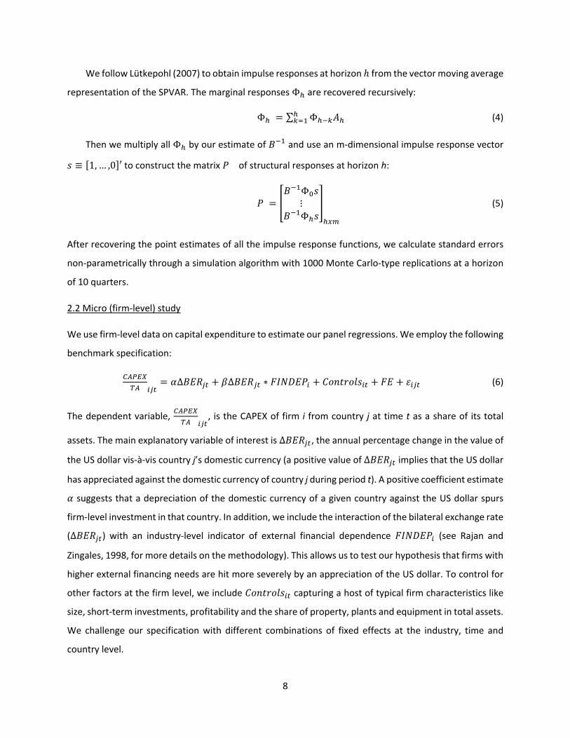
We follow Lütkepohl (2007) to obtain impulse responses at horizon ℎ from the vector moving average

representation of the SPVAR. The marginal responses Φ are recovered recursively: Φ = ∑ Φ (4)

Then we multiply all Φ by our estimate of and use an m-dimensional impulse response vector ≡ 1,… ,0 ′ to construct the matrix of structural responses at horizon h:

= Φ⋮Φ (5)

After recovering the point estimates of all the impulse response functions, we calculate standard errors

non-parametrically through a simulation algorithm with 1000 Monte Carlo-type replications at a horizon

of 10 quarters.

2.2 Micro (firm-level) study

We use firm-level data on capital expenditure to estimate our panel regressions. We employ the following

benchmark specification:

= ∆ + ∆ ∗ + + + (6)

The dependent variable, , is the CAPEX of firm i from country j at time t as a share of its total

assets. The main explanatory variable of interest is ∆ , the annual percentage change in the value of

the US dollar vis-à-vis country j’s domestic currency (a positive value of ∆ implies that the US dollar

has appreciated against the domestic currency of country j during period t). A positive coefficient estimate

suggests that a depreciation of the domestic currency of a given country against the US dollar spurs

firm-level investment in that country. In addition, we include the interaction of the bilateral exchange rate

(∆ ) with an industry-level indicator of external financial dependence (see Rajan and

Zingales, 1998, for more details on the methodology). This allows us to test our hypothesis that firms with

higher external financing needs are hit more severely by an appreciation of the US dollar. To control for

other factors at the firm level, we include capturing a host of typical firm characteristics like

size, short-term investments, profitability and the share of property, plants and equipment in total assets.

We challenge our specification with different combinations of fixed effects at the industry, time and

country level.

9

We also examine a specification in which we replace the bilateral exchange rate with the component of

the annual percentage change in the US dollar nominal effective exchange rate (NEER) index that is

unrelated (ie orthogonal) to the change in the bilateral exchange rate ( ):

= ℎ + ℎ ∗ + ℎ + + + (7)

Finally, we examine a specification in which we let both exchange rate concepts (the bilateral rate and the

broad dollar index) enter simultaneously.

= ∆ + ℎ + ∆ + ℎ ∗ + ℎ+ + + (8)

After estimating our baseline specifications for the full sample, we re-run it for different subsamples

in order to isolate firms operating in the non-tradable sector and those located in countries with a floating

exchange rate regime.

In an earlier work, Bruno and Shin (2014) find that global liquidity influences corporate risk-taking

across regions and across industry sectors. In particular, more accommodative credit conditions

associated with global liquidity at the centre lead to lower risk-adjusted lending rates that induce firms to

apply lower discount rates (and hence higher net present values) in their investment decisions. Other

things being equal, firms take on more investment projects for any given profile of expected fundamental

cash flows. In this way, global factors can induce co-movements in risk-taking and they induce greater

synchronisation of risk-taking across regions and sectors.

3. Data

Table 1 provides the descriptive statistics of all variables used to conduct our benchmark macro (country-

level) and micro (firm-level) analysis.

Panel A contains a summary for the variables used in the macro analysis, which is based on quarterly

data from Q2 2001 to Q4 2016 for a sample of 34 EMEs3.

For our benchmark exchange rate variable, we draw on quarterly averages of daily values of the

bilateral exchange rate between the domestic currency of the borrowing country and the US dollar. An

increase in the exchange rate variable indicates an appreciation of the US dollar relative to the local

3 Appendix A provides a list of all country groups used in our macro- and micro-level empirical analyses.

10

currency. We then compare the results obtained using the bilateral exchange rate versus the US dollar

against the results generated using an alternative measure of US dollar strength – the BIS broad US dollar

NEER index.

We obtain the series on US dollar-denominated cross-border bank flows from the BIS locational

banking statistics (LBS). They capture outstanding claims and liabilities of banks located in BIS reporting

countries, including intragroup positions between offices of the same banking group (BIS, 2015). The BIS

LBS are compiled following principles that are consistent with the balance of payments framework. To

take exchange-rate fluctuations and breaks-in-series into account, adjusted changes in amounts

outstanding are calculated as an approximation for flows. Most importantly for our empirical

investigation, the BIS LBS provide information about the currency composition of cross-border claims,

which allows us to isolate the US dollar-denominated component of cross-border bank lending.

Furthermore, we exploit the BIS LBS breakdowns by borrower country and sector and link them to the

changes in gross fixed capital formation as reported for the private sector in a given counterparty country.

Since the main monetary policy rates in advanced economies were stuck at the zero lower bound for

large parts of our benchmark period, we use shadow rates as a measure of the US Federal Reserve’s

monetary policy stance. More concretely, we use quarterly changes in those shadow policy rates as

described in Krippner (2015). Krippner’s shadow rate estimates are based on a two-factor model which is

shown to be more stable over time than the alternative, three-factor model. There are some concerns

that the estimated level of the shadow rate may not be a perfect measure of monetary policy stance as it

is sensitive to the assumption underlying the specification. However, changes in shadow rates – the focus

of this project – are shown to be a consistent and effective proxy for monetary policy changes.

For our aggregate investment variable, we use the country-level series on gross fixed (private) capital

formation from the IMF International Financial Statistics and World Economic Outlook.

We use the VIX as proxy for global financial market conditions. We obtain those data series from the

CBOE website. In order to match the frequency of the other variables in our benchmark empirical

specification, we convert the daily VIX data into quarterly averages.

11

Descriptive statistics Table 1

Obs. Mean Std Dev 1st percentile 99th percentile PANEL A: Variables used in the macro analysis

irate (percentage points) 1,893 -0.058 0.675 -1.699 1.898

BER_ave (%) 1,893 0.637 4.656 -7.836 19.516

BER_end (%) 1,893 0.625 5.341 -10.155 19.658

∆NEER 1,893 -0.009 2.848 -7.180 8.280

XB_Claims (%) 1,893 2.269 14.736 -34.959 66.533

ln_GFCF (%) 1,893 1.861 10.529 -30.240 25.214

ln_vix 1,893 2.931 0.356 2.433 3.787

FRB_EME_USD_index (%) 1,893 0.039 2.674 -6.499 8.162

Macro_EME_USD (%) 1,893 1.757 5.273 -5.865 29.037

PANEL B: Variables used in the micro analysis CAPEX/TA 121,632 0.620 0.071 0.001 0.419 Size 121,632 4.684 2.157 -5.286 13.353 Cash/TA 121,632 0.124 0.141 0.003 0.760 PPE/TA 121,632 0.351 0.227 0.010 0.922 ROA 121,632 4.139 6.866 -25.935 27.816

Panel A shows descriptive statistics for the quarterly variables used in the macro-level analysis. irate denotes quarterly changes in the US federal funds rate up until Q4 2007 and quarterly changes in Krippner’s (2015) shadow short rate after Q1 2008. BER_ave denotes percentage changes in the average bilateral exchange (BER_end refers to end-quarter data), ∆NEER refers to quarterly changes in the BIS broad USD nominal effective exchange rate (NEER) index, XB_Claims indicates quarterly percentage changes in cross-border, US-dollar denominated claims on country i, ln_GFCF denotes quarterly growth rates in gross-fixed capital formation and ln_vix stands for log levels of the CBOE option-implied S&P 500 volatility index from the CBOE. Changes in the bilateral exchange rates and in cross-border lending are winsorised at the 1% level in each tail of the distribution. FRB_EME_USD_index is a trade-weighted average of the foreign exchange value of the US dollar against the following set of EMEs: Mexico, China, Taiwan, Korea, Singapore, Hong Kong, Malaysia, Brazil, Thailand, Philippines, Indonesia, India, Israel, Saudi Arabia, Russia, Argentina, Venezuela, Chile and Colombia. Macro_EME_USD is trade-weighted average of the foreign exchange value of the US dollar against the set of EMEs included in the macro study (listed in Appendix A). Period covered: Q2 2001–Q3 2016. Panel B provides descriptive statistics for the annual variables used in the micro-level analysis. CAPEX/TA is defined as a firm’s capital expenditure (CAPEX) as a share of its total assets. Size is the logarithm of total assets (in USD), Cash/TA is Cash and other short-term investments scaled by total assets, PPE/TA is property, plant and equipment scaled by total assets and ROA is a measure of profitability (return on assets). Scaled capital expenditure is winsorised at the 1% and 99% level in each tail. Period covered: 2000–2015. Sources: Krippner (2015); Board of Governors of the Federal Reserve System; Federal Reserve Bank of St Louis FRED; IMF International Financial Statistics and World Economic Outlook; Chicago Board Options Exchange; national data; BIS locational banking statistics; Bloomberg; Capital IQ; authors’ calculations.

Panel B of Table 1 contains a summary for the variables used in the micro-level analysis, which exploits

annual data from Capital IQ based on firm-level reports from 32 EMEs for the period between 2000 and

2015. Besides firm-level CAPEX, which is used as our key dependent variable, we use basic firm

characteristics such as size as measured by total assets (TA), cash holdings, profitability measures (return

on assets (ROA)) and other fixed assets (property, plant and equipment). Our sample consists exclusively

of non-financial firms. To examine whether financial dependence amplifies the exchange rate effect, we

utilise an updated version of the industry-level index of external financial dependence, originally

12

developed by Rajan and Zingales (1998). All other independent variables, like the bilateral exchange rate,

the VIX and the measure of US monetary policy correspond to those used in the macro-level analysis.

4. Benchmark results

The results from both of our main empirical exercises (the macro (country-level) study and the micro (firm-

level) study) strongly suggest that an appreciation of the US dollar is associated with slowing investment

on a global scale. In the rest of this section, we discuss the key results from our two benchmark empirical

exercises. We start with the main results from the macro (country-level) SPVARs. We then discuss the key

findings from the micro (firm-level) panel regressions.

4.1 Results from the macro (country-level) study

We conduct our macro exercise using the SPVAR methodology described in Section 2.1. In our benchmark

estimation, we follow Bruno and Shin (2015a) when ordering the five endogenous variables in our SPVAR

system. It is important to note that we order cross-border bank lending ahead of the strength of the US

dollar exchange rate. This rules out any contemporaneous effects of the US dollar on cross-border bank

lending, thus tilting the odds against us finding evidence in support of the predictions of the theoretical

model of Bruno and Shin (2015b).

Figure 1 presents the key impulse responses from our benchmark SPVAR estimation. The left-hand

panel shows that a strengthening in the dollar is associated with a fall in dollar-denominated cross-border

bank lending. This finding is in line with the conclusions of Bruno and Shin (2015a, 2015b). In turn, the

centre panel of Figure 1 reveals that an increase in cross-border US dollar bank lending to a given country

boosts real investment activity in that country. This effect goes beyond simply financing real investment

with dollars – the financial channel of exchange rates generates broader incentives to take or shy away

from risks associated with currency fluctuations. This channel is especially powerful when currency

movements cause the value of borrowers’ assets or debts to grow or shrink. At the same time, the

exchange-rate fluctuations of the local currency vis-à-vis the US dollar impact the risk premium of local

currency sovereign bonds (Hofmann et al, 2016), and hence shape domestic financial conditions more

generally.

The right-hand panel presents our key finding – a US dollar appreciation affects investment, but in

the opposite direction to the trade channel. When the domestic currency weakens against the dollar,

there is a sharp drop in investment. Thus, a stronger dollar dampens economic activity, rather than

stimulating it. More concretely, a one standard deviation appreciation in the value of the US dollar vis-à-

13

vis the local currency leads to a five percentage point decline in the growth rate of gross capital formation

in the subsequent quarter. The effect emerges during the first quarter after a US dollar appreciation and

remains statistically significant for more than two years.

Impulse response functions: US dollar, cross-border bank lending, investment

Benchmark SPVAR, full sample Figure 1

US dollar on cross-border bank lending

Cross-border bank lending on capital expenditure

US dollar on capital expenditure

Black lines show the estimated impulse response functions to a one-standard-deviation shock to the exchange rate equation using a Cholesky decomposition. The SPVAR’s five endogenous variables follow the order (1) US interest rate, (2) US dollar-denominated cross-border bank flows, (3) gross capital formation, (4) bilateral average US dollar exchange rate and (5) the VIX. All variables are expressed in percentage changes except for the VIX, which enters the SPVAR in log-levels. Confidence bands reflect 95% confidence intervals using a Gaussian approximation based on 1,000 Monte Carlo draws from the estimated SPVAR. Period covered: Q2 2001–Q3 2016, based on 34 EMEs. For more information on the SPVAR, see Section 2.1.

Sources: IMF International Financial Statistics and World Economic Outlook; national data; BIS locational banking statistics; Capital IQ; Bloomberg; authors’ calculations.

In sum, the impulse response functions generated by the benchmark SPVAR analysis provide strong

evidence that the financial channel of exchange rates points in the opposite direction relative to the trade

channel. Intuitively, a stronger US dollar deteriorates the creditworthiness of currency-mismatched EME

borrowers, as their liabilities increase relative to their assets. For instance, suppose that an EME borrower

has local currency assets and dollar-denominated liabilities. Even if assets generate dollar-denominated

cash flows, a stronger dollar weakens the borrower’s cash flows due to the rising debt service costs, as in

the case of oil firms. From the standpoint of creditors, the weaker credit position of the borrower

increases tail risk in the credit portfolio and decreases the capacity for additional credit extension, even

with a fixed exposure limit through a VaR constraint or economic capital constraint. This leads to a decline

in cross-border bank lending. Bruno and Shin (2015a, 2015b) have labelled this the “risk-taking channel of

currency appreciation”. As our benchmark results illustrate, the decline in cross-border lending triggered

0.0

–0.5

–1.0

–1.5

–2.010987654321

1.2

0.8

0.4

0.0

–0.410987654321

0.0

–1.5

–3.0

–4.5

–6.010987654321

14

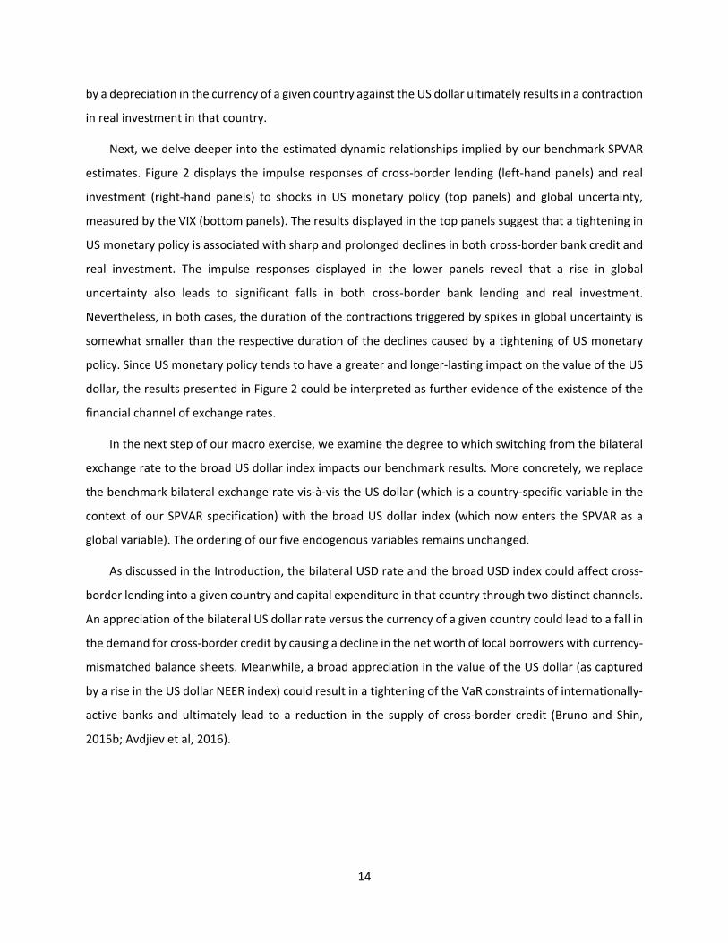
by a depreciation in the currency of a given country against the US dollar ultimately results in a contraction

in real investment in that country.

Next, we delve deeper into the estimated dynamic relationships implied by our benchmark SPVAR

estimates. Figure 2 displays the impulse responses of cross-border lending (left-hand panels) and real

investment (right-hand panels) to shocks in US monetary policy (top panels) and global uncertainty,

measured by the VIX (bottom panels). The results displayed in the top panels suggest that a tightening in

US monetary policy is associated with sharp and prolonged declines in both cross-border bank credit and

real investment. The impulse responses displayed in the lower panels reveal that a rise in global

uncertainty also leads to significant falls in both cross-border bank lending and real investment.

Nevertheless, in both cases, the duration of the contractions triggered by spikes in global uncertainty is

somewhat smaller than the respective duration of the declines caused by a tightening of US monetary

policy. Since US monetary policy tends to have a greater and longer-lasting impact on the value of the US

dollar, the results presented in Figure 2 could be interpreted as further evidence of the existence of the

financial channel of exchange rates.

In the next step of our macro exercise, we examine the degree to which switching from the bilateral

exchange rate to the broad US dollar index impacts our benchmark results. More concretely, we replace

the benchmark bilateral exchange rate vis-à-vis the US dollar (which is a country-specific variable in the

context of our SPVAR specification) with the broad US dollar index (which now enters the SPVAR as a

global variable). The ordering of our five endogenous variables remains unchanged.

As discussed in the Introduction, the bilateral USD rate and the broad USD index could affect cross-

border lending into a given country and capital expenditure in that country through two distinct channels.

An appreciation of the bilateral US dollar rate versus the currency of a given country could lead to a fall in

the demand for cross-border credit by causing a decline in the net worth of local borrowers with currency-

mismatched balance sheets. Meanwhile, a broad appreciation in the value of the US dollar (as captured

by a rise in the US dollar NEER index) could result in a tightening of the VaR constraints of internationally-

active banks and ultimately lead to a reduction in the supply of cross-border credit (Bruno and Shin,

2015b; Avdjiev et al, 2016).

15

Impulse response functions: US rates, VIX, cross-border bank lending, investment

Benchmark SPVAR, full sample Figure 2

US interest rate on cross-border bank lending US interest rate on capital expenditure

VIX on cross-border bank lending VIX on capital expenditure

Black lines show the estimated impulse response functions to a one-standard-deviation shock using a Cholesky decomposition. The SPVAR’s five endogenous variables follow the order (1) US interest rate, (2) US dollar-denominated cross-border bank flows, (3) gross capital formation, (4) bilateral average US dollar exchange rate and (5) the VIX. All variables are expressed in percentage changes except for the VIX, which enters the SPVAR in log-levels. Confidence bands reflect 95% confidence intervals using a Gaussian approximation based on 1,000Monte Carlo draws from the estimated SPVAR. Period covered: Q2 2001–Q3 2016, based on 34 EMEs. For more information on the SPVAR, see Section 2.1.


The impulse response functions presented in Figure 3 suggest that the effects of a rise in the broad

US dollar index are broadly similar to those of an appreciation in the bilateral US dollar exchange rate.

Namely, the US dollar index has a negative, statistically significant and persistent impact on real

investment in EMEs.

Nevertheless, there is also an important difference between the two sets of results. When the

bilateral exchange rate is used, the impact of cross-border bank lending on capital expenditure is

statistically significant only contemporaneously (Figure 1, centre panel). The statistical significance

0.0

–1.3

–2.5

–3.8

–5.010987654321

0.0

–1.3

–2.5

–3.8

–5.010987654321

0.0

–1.0

–2.0

–3.0

–4.010987654321

0.0

–1.0

–2.0

–3.0

–4.010987654321

16

disappears in subsequent periods. By contrast, when the broad US dollar index is used, the (statistically

significant) effect is much longer-lasting (Figure 3, centre panel). This set of results implies that the cross-

border credit supply channel highlighted in Avdjiev et al (2016) tends to be stronger and more persistent

than the standard credit demand channel emphasised by the EME crisis literature.


Alternative SPVAR (using broad US dollar index instead of bilateral rate), full sample Figure 3




Black lines show the estimated impulse response functions to a one-standard-deviation shock to the exchange rate using a Cholesky decomposition. The SPVAR’s five endogenous variables follow the order (1) US interest rate, (2) US dollar-denominated cross-border bank flows, (3) gross capital formation, (4) BIS USD NEER broad index and (5) the VIX. All variables are expressed in percentage changes except for the VIX, which enters the SPVAR in log-levels. Confidence bands reflect 95% confidence intervals using a Gaussian approximation based on1,000 Monte Carlo draws from the estimated SPVAR. Period covered: Q2 2001–Q3 2016, based on 34 EMEs. For more information on the SPVAR, see Section 2.1.


Furthermore, we examine the degree to which our benchmark results are driven by specific time

periods within our benchmark sample window. More concretely, we examine four subsample time

windows defined by two critical points in the recent history of the global financial system – the peak of

the Global Financial Crisis (Q3 2008) and the point in time after which the high correlation between the

US dollar and the VIX started to weaken (Q3 2012).

The key impulse response functions for the above four time windows are presented in Figure 4. They

reveal that the strong negative relationship between the value of the US dollar and real investment is

present in all individual sub-periods within our sample. The estimated impact was a bit larger and longer-

lasting before the crisis than during the post-crisis period. The pre-crisis impact peaked at about -6% and

lasted for roughly two years (top left-hand panel), while the post-crisis impact peaked at about -4.5% and

0.0

–0.7

–1.4

–2.1

–2.810987654321

1.2

0.8

0.4

0.0

–0.410987654321

0.0

–1.0

–2.0

–3.0

–4.010987654321

17

lasted for about a year (top right-hand panel). The estimated effect between 2001 and 2012 is even larger,

reaching its highest level at almost -7% (bottom left-hand panel). Finally, although the impact during the

post-2012 subsample is not as large as its pre-2012 counterpart, it is still very sizeable (peaking at roughly

-4%) and strongly statistically significant for several quarters after the initial shock (bottom right-hand

panel).

Impulse response functions: US dollar on capital expenditure

Benchmark SPVAR, alternative time windows Figure 4

Q1 2001–Q2 2008 Q4 2008–Q3 2016

Q1 2001–Q3 2012 Q4 2012–Q3 2016

Black lines show the estimated impulse response functions to a one-standard-deviation shock to the exchange rate using a Cholesky decomposition. The SPVAR’s five endogenous variables follow the order (1) US interest rate, (2) US dollar-denominated cross-border bank flows, (3) gross capital formation, (4) bilateral average US dollar exchange rate and (5) the VIX. All variables are expressed in percentage changes except for the VIX, which enters the SPVAR in log-levels. Confidence bands reflect 95% confidence intervals using a Gaussian approximation based on 1,000 Monte Carlo draws from the estimated SPVAR, based on 34 EMEs. For more information on the SPVAR, see Section 2.1.


0.0

–1.9

–3.8

–5.6

–7.510987654321

0.0

–1.9

–3.8

–5.6

–7.510987654321

0.0

–1.9

–3.8

–5.6

–7.510987654321

0.0

–1.9

–3.8

–5.6

–7.510987654321

18

4.2 Results from the micro (firm-level) study

We conduct our micro (firm-level) empirical examination of the impact of the US dollar exchange rate on

real investment using the panel regression setup described in Section 2.2.

Table 2 reports the benchmark panel regressions for firm-level CAPEX variable for a sample of 32

countries over the period between 2000 and 2015. Column 1 shows that the coefficient estimate of the

bilateral exchange rate (ΔBER) is positive and statistically significant. Hence, a depreciation of the local

currency spurs competitiveness and firms’ investments. This finding reflects the standard textbook

competitiveness channel.

Benchmark regression results of CAPEX/TA

Firms in the full sample Table 2

(1) (2) (3) ∆BER 0.0168*** 0.0123***

(0.0032) (0.0032)

∆NEERorth -0.1598*** -0.1220***

(0.0243) (0.0239)

Size -0.0004** -0.0004** -0.0004**

(0.0002) (0.0002) (0.0002)

Cash/TA 0.0184*** 0.0183*** 0.0183***

(0.0019) (0.0019) (0.0019)

PPE/TA 0.1353*** 0.1354*** 0.1353***

(0.0020) (0.0021) (0.0021)

ROA 0.0014*** 0.0014*** 0.0014***

(0.0001) (0.0000) (0.0000)

Constant -0.0032 0.0006 -0.0012

(0.0065) (0.0086) (0.0086)

Year FE Y Y Y

Country FE Y Y Y

Industry FE Y Y Y

Observations 121,632 121,632 121,632

R-squared 0.208 0.208 0.208This table reports OLS results with industry, year, country and country-year dummies where the dependent variable is firm-level capital expenditure scaled by total assets. Exchange rate (∆BER) is the annual percentage change in the value of the dollar vis-à-vis the local currency. Size is the logarithm of total assets (in USD), Cash/TA is Cash and other short-term investments scaled by total assets, PPE/TA is property, plant and equipment scaled by total assets and ROA is return on assets. Non-tradable sectors refers to the all the industries except the following two-digit SIC codes (tradable sectors): 1 to 14 (agriculture, oil and mining), 20 to 39 (manufacturing). ∆NEERorth is the component of the annual percentage change in the US dollar NEER index that is unrelated (ie orthogonal) to the change in the bilateral exchange rate. All regressions include country, industry and year fixed effects. Standard errors are either adjusted at the firm level or, if the number of firm-level clusters is too small, at the country level. We report standard errors in parentheses.

Sources: BIS; Capital IQ;

19

Next, we compare the estimated impact of the bilateral exchange rate to that of the broad US dollar

index. To address collinearity concerns, we use the component of the broad US dollar index that is

unrelated (ie orthogonal) to the change in the bilateral exchange rate (ΔNEERorth), defined as the residuals

obtained from regressing the broad US dollar index on the bilateral exchange rate.

When we use the orthogonal component of the broad US dollar index instead of the bilateral rate

(ΔBER), its estimated coefficient is negative and statistically significant (column 2).4

In column 3, we report the results from a specification in which we simultaneously include both the

bilateral exchange rate and the orthogonal component of the broad US dollar index. The coefficient of the

bilateral exchange rate (ΔBER) remains positive and statistically significant, while the coefficient of the

broad US dollar residuals (ΔNEERorth) remains negative and statistically significant.

Taken together, the above results suggest that, for the full sample, a strengthening of the broad US

dollar index has the opposite effect on firms’ investments than an appreciation of the US dollar’s bilateral

exchange rate vis-à-vis the local currency. The estimated impact of the former is negative, while that of

the latter is positive. We delve deeper into this dichotomy using the next set of regressions.

In Table 3, we restrict the analysis to the subsample of non-tradable sectors in countries with floating

exchange rate regimes. Non-tradable sectors refers to all the industries except the following two-digit SIC

codes: 1 to 14 (agriculture, oil and mining), 20 to 39 (manufacturing). The classification of the countries

exchange rate arrangements is from the IMF Annual Report on Exchange Arrangements and Exchange

Restrictions.

The results reported in column 1 reveal that the coefficient of the bilateral exchange rate is no longer

statistically significant for this subset of firms.

In column 2, we interact the bilateral exchange rate with an industry-level indicator of external

financial dependence (FINDEP). The interaction coefficient of the bilateral exchange rate with FINDEP is

negative and statistically significant. This implies that the reduction in investment triggered by a US dollar

appreciation is greater for firms that are more dependent on external financing. The magnitude of the

effect is large: a one percentage point increase in the bilateral value of the US dollar reduces the capital

4 When we use the broad US dollar index (instead of its orthogonal component), its coefficient estimate is also negative and statistically significant. The results from that additional specification are available upon request.

20

expenditure ratio by 0.003 (5.5% of the sample mean) more in industries at the 66th percentile than in

industries at the 33rd percentile of the FINDEP index.5

5 In results that are available upon request, we find that the above evidence does not apply to firms in tradable sectors. A dollar appreciation leads to higher real investment by firms in tradable sectors, which is consistent with the trade channel.

Benchmark regression results of CAPEX/TA

Firms in non-tradable sectors and floating exchange rate regime countries Table 3

(1) (2) (3) (4) (5) (6)

∆BER 0.0005 0.0074 -0.0084 0.0011

(0.0078) (0.0088) (0.0075) (0.0136)

∆NEERorth -0.3043*** -0.4268**

(0.0799) (0.1903)

∆BER * FINDEP -0.0208** -0.0241*** -0.0243** -0.0203***

(0.0105) (0.0072) (0.0088) (0.0060)

∆NEERorth * FINDEP 0.3597 0.3612

(0.2368) (0.2449)

Size -0.0009** -0.0009** -0.0009** -0.0009 -0.0008 -0.0008

(0.0004) (0.0004) (0.0004) (0.0012) (0.0013) (0.0013)

Cash/TA 0.0089** 0.0086** 0.0089** 0.0085 0.0076 0.0078

(0.0041) (0.0041) (0.0041) (0.0066) (0.0066) (0.0065)

PPE/TA 0.1364*** 0.1366*** 0.1364*** 0.1368*** 0.1364*** 0.1363***

(0.0043) (0.0043) (0.0043) (0.0120) (0.0118) (0.0117)

ROA 0.0002 0.0001 0.0002 0.0001 0.0001 0.0001

(0.0001) (0.0001) (0.0001) (0.0005) (0.0005) (0.0005)

Constant -0.0210** -0.0421 -0.0207** -0.0380* -0.0108 -0.0137

(0.0102) (0.0302) (0.0102) (0.0213) (0.0176) (0.0187)

Year FE Y Y Y Y N N

Country FE Y Y Y Y N N

Industry FE Y Y Y Y Y Y

Country-year FE N N N N Y Y

Observations 20,877 20,818 20,877 20,818 20,818 20,818

R-squared 0.215 0.215 0.215 0.215 0.221 0.220 This table reports results from the same type of regressions as Table 2, but restricted to the sample of firms in non-tradable sectors and countries with floating regimes. FINDEP is an industry-level indicator of external financial dependence (as defined in Rajan and Zingales,1998). All other variables are defined as in Table 2. Standard errors are adjusted at the firm level and are reported in parentheses.

Sources: BIS; Capital IQ; Compustat.

21

Next, we add the orthogonal component of the broad US dollar index (ΔNEERorth) to the main

specification (column 3). The coefficient on the broad US dollar index is negative and statistically

significant, while the coefficient of the bilateral exchange rate remains statistically insignificant.

We then interact both exchange rates with FINDEP and include country and year dummies (column

4) or country-year (column 5) fixed effects. The coefficient of the interaction term ΔBER*FINDEP is

negative and statistically significant, whereas the coefficient of the interaction term ΔNEERorth*FINDEP is

statistically insignificant. Column 6 confirms that the negative and statistically significant coefficient on

the interaction term ΔBER*FINDEP is robust to using country-year and industry fixed effects. Taken

together, the above results suggest that on average there is a global dollar credit supply effect that

dominates the local credit demand effect (ΔBER is statistically insignificant, whereas ΔNEERorth is negative

and statistically significant).6 However, when we consider individual firms’ external financing needs, the

interaction term ΔBER *FINDEP is negative and statistically significant, which implies that the reduction in

investment triggered by a US dollar appreciation is greater for firms that are more dependent on external

financing, ie those firms that demand more external funds.

Table 4 presents the results from supplementary specifications that examine several additional

(country group and time period) splits of the subsample of firms in non-tradable sectors and in floating

exchange rate regime countries. We start with a specification that includes country-year fixed effects and

split the sample into a pre- and a post-2011 period. Column 1 of Table 4 shows that the negative

coefficient of the interaction term between exchange rate and external financial dependence is driven by

the post-2011 period, when the dollar borrowing by non-financial corporates in emerging markets rose

significantly. Accordingly, column 2 confirms that the evidence is weaker before 2011.

When we further split the sample between firms in emerging Asia and emerging Europe, we see that

the negative coefficient is large in magnitude and statistically significant for emerging Asia (column 3), but

not for emerging Europe (column 4). Finally, column 5 shows that our results are robust to additional

country-level control variables.

6 In order to compare the economic impacts of the two types of exchange rates, the bilateral exchange rate vis-à-vis the US dollar and the broad nominal US dollar index, we run the baseline specifications including each of them (one at a time), without year fixed effects. The coefficient estimate of the bilateral exchange rate is -0.021, while that on the broad US dollar index is -0.09. Those estimates imply that the impact of the broad dollar index on capital expenditures is roughly four times larger than the respective impact of the bilateral exchange rate.

22

Regression results of CAPEX/TA, alternative subsamples

Firms in non-tradable sectors and in floating exchange rate regime countries Table 4

(1) (2) (3) (4) (5) Post-2011 Pre-2011 Emerging Asia Emerging Europe Full sample

∆BER 0.0099 (0.0099)

∆BER * FINDEP -0.0219*** -0.0240 -0.0591** 0.0250 -0.0247** (0.0059) (0.0192) (0.0166) (0.0362) (0.0109)

Size -0.0011 -0.0003 0.0004 -0.0069*** -0.0005 (0.0010) (0.0019) (0.0003) (0.0019) (0.0004)

Cash/TA 0.0090 0.0020 -0.0094 0.0000 0.0065 (0.0073) (0.0051) (0.0051) (0.0068) (0.0043)

PPE/TA 0.1272*** 0.1630*** 0.1429*** 0.1100*** 0.1418*** (0.0054) (0.0282) (0.0068) (0.0083) (0.0046)

ROA -0.0001 0.0008*** 0.0011*** 0.0008*** 0.0003*** (0.0005) (0.0002) (0.0001) (0.0001) (0.0001)

MarketCap/GDP 0.0142** (0.0059)

Stock price 0.0766*** (0.0231)

GDP per capita -0.0346* (0.0196)

Constant -0.0894*** -0.0121 -0.0909*** 0.0892*** 0.2463 (0.0171) (0.0235) (0.0052) (0.0230) (0.1783)

Year FE N N N N Y

Country FE N N N N Y

Industry FE Y Y Y Y Y

Country-year FE Y Y Y Y N

Observations 14,798 6,020 5,810 1,715 17,688

R-squared 0.200 0.297 0.257 0.215 0.228 This table reports results from the same type of regressions as Table 2, but restricted to the sample of firms in non-tradable sectors and countries with floating regimes. It also uses the following additional firm-level control variables: Stock market capitalisation to GDP in % (MarketCap/GDP), Stock price volatility, GDP per capita; all other variables are defined as in Table 2. Standard errors are either adjusted at the firm level or, if the number of firm-level clusters is too small, at the country level, and are reported in brackets. Sources: BIS; World Bank Global Development Database; Capital IQ; Compustat.

23

5. Robustness analysis

We examine the robustness of our key results by estimating a number of alternative specifications for

both our macro SPVARs and our micro panel regressions.

5.1 Robustness tests for the macro study

In theory, there could be an alternative explanation for our benchmark results. Namely, during periods in

which the risk-adjusted returns associated with investing in EMEs are high, global investors (including

internationally-active banks) would be more likely to engage in carry trade activities, shorting US dollar

assets and going long in EME assets. This would increase the supply of US dollars in global FX markets and

ultimately lead to a depreciation of the US dollar.

In order to test the above hypothesis, we add a variable that captures carry trade incentives to our

SPVAR. More specifically, we use the Bloomberg carry trade index, which is defined as the cumulative

total return of a buy-and-hold carry trade position that is funded with short positions in the US dollar and

that is long in eight emerging market currencies.7 We place the EME carry trade index in the second

position in the SPVAR ordering, ahead of cross-border bank flows and gross capital formation, thus

allowing it to impact both of the latter variables contemporaneously. This SPVAR ordering stacks the odds

in favour of the “carry trade activity” hypothesis and against our main hypothesis.

The key impulse responses generated by the above six-variable SPVAR system are presented in Figure

5. They provide further evidence in support of our main hypothesis. Just as in our benchmark results

(displayed in Figure 1), a US dollar appreciation has a negative and statistically significant impact on cross-

border bank lending (left-hand panel), which in turn has a positive and statistically significant impact on

capital expenditure (centre panel). The combination of the above two dynamic patterns once again

generates our main result – an appreciation in the value of the US dollar leads to a statistically significant

contraction in capital formation.

7 The following currencies enter the Bloomberg carry trade index: Brazilian real, Mexican peso, Indian rupee, Indonesian rupiah, South African rand, Turkish lira, Hungarian forint and Polish zloty. We compute percentage changes of quarterly averages constructed using monthly data.

24


Six-variable SPVAR (adding the carry trade index), full sample Figure 5




Black lines show the impulse responses to a one-standard-deviation shock to the exchange rate using a Cholesky decomposition. The SPVAR’s six endogenous variables follow the order (1) US interest rate, (2) carry trade index, (3) US dollar-denominated cross-border bank flows, (4) gross capital formation, (5) bilateral average US dollar exchange rate and (6) the VIX. All variables are expressed in percentage changes except for the VIX, which enters the SPVAR in log-levels. Confidence bands reflect 95% confidence intervals using a Gaussian approximation based on 1,000 Monte Carlo draws from the estimated SPVAR. Period covered: Q2 2001–Q3 2016, based on 34 EMEs. For more information on the SPVAR, see Section 2.1.


Next, we test the robustness of our results to the ordering in the SPVAR system. More concretely, we

move the US dollar exchange rate variable to the second position, ahead of cross-border bank flows and

gross capital formation. This ordering allows the US dollar exchange rate to have a contemporaneous

impact on the latter two variables, thus also addressing the possibility of any persistent carry trade

dynamics. We perform the above robustness check for both the SPVAR system which includes the bilateral

US dollar rate and the system that includes the broad US dollar NEER index, instead.

Figures 6 and 7 display the key impulse responses generated by the above alternatively-ordered

SPVARs. They reveal that our benchmark results are robust. Namely, a US dollar appreciation leads to a

decline in cross-border lending (left-hand panels). Furthermore, in both cases (for the bilateral US dollar

exchange rate and the for the broad US dollar NEER index), the estimated contractions are even deeper

and more persistent than their counterparts in the benchmark specifications (in Figures 1 and 3,

respectively). Similarly, in both alternative estimations, a US dollar appreciation shock causes a sharp fall

in capital expenditure (right-hand panels of Figures 6 and 7).

0.8

0.0

–0.8

–1.6

–2.410987654321

1.0

0.5

0.0

–0.5

–1.010987654321

0.0

–1.3

–2.6

–3.9

–5.210987654321

25


Alternative SPVAR (ordering the bilateral exchange rate in second position), full sample Figure 6




Black lines show the impulse responses to a one-standard-deviation shock to the exchange rate using a Cholesky decomposition. The SPVAR’s five endogenous variables now follow the order (1) US interest rate, (2) bilateral average US dollar exchange rate, (3) US dollar-denominated cross-border bank flows, (4) gross capital formation and (5) the VIX. All variables are expressed in percentage changes except for the VIX, which enters the SPVAR in log-levels. Confidence bands reflect 95% confidence intervals using a Gaussian approximation based on 1,000 Monte Carlo draws from the estimated SPVAR. Period covered: Q2 2001–Q3 2016, based on 34 EMEs. For more information on the SPVAR, see Section 2.1.



Alternative SPVAR (ordering the USD NEER in second position), full sample Figure 7




Black lines show the impulse responses to a one-standard-deviation shock to the exchange rate using a Cholesky decomposition. The SPVAR’s five endogenous variables now follow the order (1) US interest rate, (2) BIS USD NEER broad index (3) US dollar-denominated cross-border bank flows, (4) gross capital formation and (5) the VIX. All variables are expressed in percentage changes except for the VIX, which enters the SPVAR in log-levels. Confidence bands reflect 95% confidence intervals using a Gaussian approximation based on 1,000 MonteCarlo draws from the estimated SPVAR. Period covered: Q2 2001–Q3 2016, based on 34 EMEs. For more information on the SPVAR, see Section 2.1.


0.0

–0.6

–1.2

–1.9

–2.510987654321

0.8

0.4

0.0

–0.4

–0.810987654321

0.0

–1.5

–3.0

–4.5

–6.010987654321

0.0

–0.8

–1.5

–2.3

–3.010987654321

1.0

0.5

0.0

–0.5

–1.010987654321

0.0

–1.0

–2.0

–3.0

–4.010987654321

26

Our benchmark results for the impact of the “broad” US dollar index draw on the US dollar NEER.

Since this is a trade-weighted index, it naturally places greater weights on the bilateral exchange rates of

the most important trading partners of the United States – Canada, Mexico, China and the euro area.

Nevertheless, for the main question we examine, what matters most are the fluctuations in the value of

the US dollar against a wider range of EME currencies.

That is why we examine the robustness of our benchmark results by replacing the US dollar NEER

with two alternative US dollar indices. The first one is the Federal Reserve Board’s EME broad US dollar

(trade-weighted) index,8 which captures fluctuations of the US dollar exclusively against EME currencies.

For the second alternative US dollar index, we construct our own (GDP-weighted) average of the value of

the US dollar against the currencies of the set of EMEs used in our benchmark macro study.

Both of the above alternative indices exhibit a highly positive and significant correlation with the US

dollar NEER index used in our benchmark macro study. The correlation coefficient between the FRB’s EME

broad dollar index and the US dollar NEER is 0.87 and is statistically significant at the 1% level. The second

alternative US dollar EME exchange rate index is also highly correlated with the US dollar NEER – although

the correlation between those two indices (0.44) is not as high as in the case of the FRB’s EME index, it is

still highly statistically significant (at the 1% level).

Figures 8 and 9 display the most important impulse responses from the SPVARs using the above two

alternative US dollar EME exchange rate indices. In both cases, the results are very similar to the ones

obtained from the benchmark specification. Namely, a US dollar appreciation has a negative impact on

cross-border bank lending (left-hand panels), which, in turn, has a positive impact on capital expenditure

(centre panels). The combination of the above two estimated impacts naturally results in the third key

estimated response – that of capital expenditure to a US dollar appreciation – which is sharply negative.

8 Formal name: Trade Weighted U.S. Dollar Index: Other Important Trading Partners.

27


Alternative SPVAR (replacing the USD NEER with the FRB EME USD index), full sample Figure 8




Black lines show the impulse responses to a one-standard-deviation shock to the exchange rate using a Cholesky decomposition. The SPVAR’s five endogenous variables follow the order (1) US interest rate, (2) US dollar-denominated cross-border bank flows, (3) gross capital formation, (4) FRB EME USD broad index and (5) the VIX. All variables are expressed in percentage changes except for the VIX, which enters the SPVAR in log-levels. Confidence bands reflect 95% confidence intervals using a Gaussian approximation based on 1,000 Monte Carlodraws from the estimated SPVAR. Period covered: Q2 2001–Q3 2016, based on 34 EMEs. For more information on the SPVAR, see Section 2.1.

Sources: IMF International Financial Statistics and World Economic Outlook; national data; BIS locational banking statistics; Capital IQ; Bloomberg; Board of Governors of the Federal Reserve System; authors’ calculations.


Alternative SPVAR (replacing the USD NEER with the GDP-weighted EME USD index), full sample Figure 9




Black lines show the impulse responses to a one-standard-deviation shock to the exchange rate using a Cholesky decomposition. The SPVAR’s five endogenous variables follow the order (1) US interest rate, (2) US dollar-denominated cross-border bank flows, (3) gross capital formation, (4) GDP-weighted EME USD exchange rate index, and (5) the VIX. All variables are expressed in percentage changes except for the VIX, which enters the SPVAR in log-levels. Confidence bands reflect 95% confidence intervals using a Gaussian approximation based on 1,000Monte Carlo draws from the estimated SPVAR. Period covered: Q2 2001–Q3 2016, based on 34 EMEs. For more information on the SPVAR, see Section 2.1.


0.0

–0.8

–1.6

–2.4

–3.210987654321

1.5

1.0

0.5

0.0

–0.510987654321

0.0

–0.8

–1.6

–2.4

–3.210987654321

0.0

–0.5

–1.0

–1.5

–2.010987654321

1.8

1.2

0.6

0.0

–0.610987654321

0.0

–0.6

–1.2

–1.8

–2.410987654321

28

Next, we restrict the EME sample of the benchmark five-variable SPVAR system to the set of EME

countries that enters our micro (firm-level) study presented in Table 2. Our specification and the order of

included endogenous variables remain unchanged. The impulse responses generated by that alternative

sample are presented in Figure 10 and reveal that our results are robust to alternative sets of borrowing

countries. Namely, the impact of the bilateral US dollar exchange rate on cross-border bank lending and

on real investment is still negative and statistically significant for at least two years after the initial

appreciation shock.


Benchmark SPVAR, sample of countries in the micro study Figure 10




Black lines show the impulse responses to a one-standard-deviation shock to the exchange rate using a Cholesky decomposition. The SPVAR’s five endogenous variables follow the order (1) US interest rate, (2) US dollar-denominated cross-border bank flows, (3) gross capital formation, (4) bilateral average US dollar exchange rate and (5) the VIX. All variables are expressed in percentage changes except for the VIX, which enters the SPVAR in log-levels. Confidence bands reflect 95% confidence intervals using a Gaussian approximation based on 1,000Monte Carlo draws from the estimated SPVAR. Period covered: Q2 2001–Q3 2016, based on 28 EMEs. For more information on the SPVAR, see Section 2.1.


Figure 11 links our macro SPVAR with the micro panel analysis by further reducing the set of

borrowing countries to those with floating exchange rate regimes (as shown in Table 3 and Table 4).

Once again, the exhibited patterns align well with the results based on the full sample.

0.0

–0.6

–1.2

–1.8

–2.410987654321

1.5

1.0

0.5

0.0

–0.510987654321

0.0

–2.0

–4.0

–6.0

–8.010987654321

29


Benchmark SPVAR, sample of countries with floating exchange rate regimes Figure 11




Black lines show the impulse responses to a one-standard-deviation shock to the exchange rate using a Cholesky decomposition. The SPVAR’s five endogenous variables follow the order (1) US interest rate, (2) US dollar-denominated cross-border bank flows, (3) gross capital formation, (4) bilateral average US dollar exchange rate and (5) the VIX. All variables are expressed in percentage changes except for the VIX, which enters the SPVAR in log-levels. Confidence bands reflect 95% confidence intervals using a Gaussian approximation based on 1,000 Monte Carlo draws from the estimated SPVAR. Period covered: Q2 2001–Q3 2016, based on 23 EMEs. For more information on the SPVAR, see Section 2.1.


Next, we return to our Section 4.1 benchmark set of borrowing EMEs, while replacing the average

quarterly bilateral exchange rate with the end-of-period quarterly bilateral exchange rate. Figure 12

shows that the estimated impulse response functions are virtually the same as their counterparts implied

by the benchmark SPVAR estimation.

We also test the extent to which the VIX as a global endogenous variable drives our benchmark SPVAR

findings. In order to do that, we replace the VIX with global GDP growth, another global variable shown

to act as an important global push factor of international capital flows by the existing empirical literature.

Figure 13 illustrates that, although the magnitude of the impact of US dollar on cross-border bank credit

and real investment declines a bit, its statistical significance and its persistence are both preserved in that

specification as well.

1.0

0.0

–1.0

–2.0

–3.010987654321

1.2

0.8

0.4

0.0

–0.410987654321

0.0

–1.5

–3.0

–4.5

–6.010987654321

30


Alternative SPVAR (replacing average BER rate with end-of-period BER rate), full sample Figure 12




Black lines show the impulse responses to a one-standard-deviation shock to the exchange rate using a Cholesky decomposition. The SPVAR’s five endogenous variables follow the order (1) US interest rate, (2) US dollar-denominated cross-border bank flows, (3) gross capital formation, (4) bilateral end-of-quarter US exchange rate and (5) the VIX. All variables are expressed in percentage changes except for the VIX, which enters the SPVAR in log-levels. Confidence bands reflect 95% confidence intervals using a Gaussian approximation based on 1,000Monte Carlo draws from the estimated SPVAR. Period covered: Q2 2001–Q3 2016, based on 34 EMEs. For more information on the SPVAR, see Section 2.1.



Alternative SPVAR (replacing VIX with global GDP growth), full sample Figure 13




Black lines show the impulse responses to a one-standard-deviation shock to the exchange rate using a Cholesky decomposition. The SPVAR’s five endogenous variables follow the order (1) US interest rate, (2) US dollar-denominated cross-border bank flows, (3) gross capital formation, (4) BIS USD NEER broad index and (5) real global GDP growth. All variables are expressed in percentage changes. Confidence bands reflect 95% confidence intervals using a Gaussian approximation based on 1,000 Monte Carlo draws from the estimated SPVAR. Period covered: Q2 2001–Q3 2016, based on 34 EMEs. For more information on the SPVAR, see Section 2.1.


0.0

–0.4

–0.8

–1.2

–1.610987654321

1.2

0.8

0.4

0.0

–0.410987654321

0.0

–0.5

–1.0

–1.5

–2.010987654321

0.0

–0.4

–0.8

–1.2

–1.610987654321

1.0

0.5

0.0

–0.5

–1.010987654321

0.0

–1.0

–2.0

–3.0

–4.010987654321

31

Finally, we examine the impact of a US dollar appreciation on overall economic activity in the

borrowing country. We do that by replacing the country-specific investment growth variable in our

benchmark SPVAR system with its country-specific GDP growth counterpart. The impulse responses,

displayed in Figure 14, reveal that an appreciation of the US dollar against the domestic currency of a

given country leads to a sharp contraction in GDP growth in that country. Even though this is followed by

a brief (one-quarter) reversal, the impact beyond the third quarter after the initial FX shock remains

negative and statistically significant for at least another year.

Impulse response functions: US dollar, cross-border bank lending, GDP growth

Alternative SPVAR (replacing investment growth with GDP growth), full sample Figure 14


Cross-border bank lending on GDP growth

US dollar on GDP growth

Black lines show the impulse responses to a one-standard-deviation shock to the exchange rate using a Cholesky decomposition. The SPVAR’s five endogenous variables follow the order (1) US interest rate, (2) US dollar-denominated cross-border bank flows, (3) real national GDP growth, (4) BIS USD NEER broad index and (5) the VIX. All variables are expressed in percentage changes except for the VIX, which enters theSPVAR in log-levels. Confidence bands reflect 95% confidence intervals using a Gaussian approximation based on 1,000 Monte Carlo drawsfrom the estimated SPVAR. Period covered: Q2 2001–Q3 2016, based on 29 EMEs. For more information on the SPVAR, see Section 2.1.


0.0

–0.8

–1.5

–2.3

–3.010987654321

1.6

0.8

0.0

–0.8

–1.610987654321

0.0

–1.3

–2.5

–3.8

–5.010987654321

32

5.2 Robustness tests for the micro (firm-level) study

Next, we conduct robustness tests for the micro specifications. More concretely, we estimate alternative

specifications with different control variables for the subsample of firms in the non-tradable sectors

located in countries with floating exchange rate regimes.

The first set of robustness results is presented in Table 5. It confirms that these subsample results are

consistent with the benchmark finding that a dollar appreciation has a contractionary effect on capital

flows and capital expenditures.

Columns 1 and 2 represent a horse race between the financial channel and the conventional savings

channel, which may be also affected by exchange rate movements. Column 1 shows that, as expected,

higher gross savings (as a percentage of GDP) are associated with higher capital expenditures.

Nevertheless, the effect is smaller for firms with higher external financial dependence – the interaction

term has a negative and statistically significant coefficient estimate. In other words, the savings channel

works in the opposite direction to the financial channel. Adding the exchange rate and its interaction with

FINDEP in column 2 confirms our previous evidence on the financial channel by providing support to the

risk-taking channel of exchange rates.

Column 3 reveals that countries with a larger proportion of external loans and deposits of reporting

banks vis-à-vis all sectors (in percent of domestic bank deposits) are associated with higher capital

expenditures for those firms that are more dependent on external financing. The negative coefficient

estimate of the interaction between the exchange rate change and FINDEP retains its statistical

significance.

In the next couple of specifications (columns 4 and 5), we also sequentially include the US interest

rate and the VIX, interacted with FINDEP. In both cases, the coefficient on the interaction term between

the exchange rate change and financial dependence remains negative and significant.

Finally, column 6 presents the estimates for the specification in which we control for the share of

bank debt (as a stand-alone variable and interacted with financial dependence). Once again, we obtain a

negative and significant coefficient on the interaction term between the exchange rate change and

FINDEP.

33

Regression results of CAPEX/TA, alternative specifications


(1) (2) (3) (4) (5) (6)

∆BER 0.0158* 0.0022 0.0073 0.0075 0.0429

(0.0091) (0.0101) (0.0088) (0.0088) (0.0803)

∆BER * FINDEP -0.0354*** -0.0193* -0.0204* -0.0213** -0.0171*

(0.0113) (0.0104) (0.0105) (0.0104) (0.0088)

ExLoans -0.0000

(0.0003)

ExLoans * FINDEP 0.0006***

(0.0002)

Savings 0.0008*** 0.0009*** (0.0003) (0.0003)

Savings * FINDEP -0.0004*** -0.0005*** (0.0001) (0.0001)

∆US rate * FINDEP 0.0007 (0.0006)

∆VIX * FINDEP 0.0020 (0.0031)

Bank debt 0.0159* (0.0087)

Bank debt * FINDEP -0.0151 (0.0808)

Size -0.0009** -0.0009** -0.0006 -0.0009** -0.0009** 0.0008 (0.0004) (0.0004) (0.0004) (0.0004) (0.0004) (0.0005)

Cash/TA 0.0090** 0.0091** 0.0068 0.0086** 0.0086** 0.0069 (0.0041) (0.0041) (0.0044) (0.0041) (0.0041) (0.0071)

PPE/TA 0.1372*** 0.1371*** 0.1419*** 0.1366*** 0.1366*** 0.1298*** (0.0043) (0.0043) (0.0046) (0.0043) (0.0043) (0.0055)

ROA 0.0001 0.0001 0.0003*** 0.0001 0.0001 0.0011*** (0.0001) (0.0001) (0.0001) (0.0001) (0.0001) (0.0001)

Constant -0.0613** -0.0749** -0.0176 -0.0368 -0.0417 -0.0535 (0.0306) (0.0309) (0.0454) (0.0302) (0.0302) (0.0367)

Observations 20,753 20,753 17,730 20,818 20,818 11,243

R-squared 0.216 0.216 0.227 0.215 0.215 0.258 This table reports results from the same type of regressions as Table 2, but restricted to the sample of firms in non-tradable sectors and countries with floating regimes. It also uses the following additional country-level control variables: external loans as % of domestic bank deposits (ExLoans), gross savings as a percentage of GDP (Savings), VIX in log differences (∆VIX), US interest rates in first differences (∆US rate) and total bank debt as a percentage of total debt (Bank debt). As in Table 2, all regression specifications include country, industry and time fixed effects. Standard errors are either adjusted at the firm level or, if the number of firm-level clusters is too small, at the country level, and are reported in brackets. Sources: World Bank; Capital IQ; Chicago Board Options Exchange; Compustat; Bank for International Settlements.

34

Table 6 presents the results from an additional set of robustness tests that we conduct. In the first

specification, we use a more granular measure for dependence on external finance. More specifically, we

use the three-digit industry measure from Claessens et al (2012). Column 1 reveals that our key results

are robust to the inclusion of this more granular measure of dependence on external finance – the

coefficient on the interaction term between the exchange rate change and FINDEP remains negative and

significant.

Next, we include country-year and industry-year fixed effects (while returning to our benchmark two-

digit SIC code FINDEP). We estimate this specification for the full sample (column 2) and for the sample

that drops the period of the global financial crisis (column 3). In both cases, our main results not only

remain intact, but also become even more statistically significant.

Finally, we re-estimate the specification reported in column 2, while controlling for firm-level

profitability with Tobin’s Q (column 4). The inclusion of this additional variable reduces the size of the

sample considerably. Nevertheless, the coefficient on the interaction term between the exchange rate

change and financial dependence remains negative and strongly statistically significant.

35

Regression results of CAPEX/TA, alternative specifications and subsamples


(1) (2) (3) (4) Full sample Full sample Excl 2008–2011 Full sample

∆BER 0.0086

(0.0098)

∆BER * FINDEP -0.0106* -0.0528*** -0.0546*** -0.0551*** (0.0057) (0.0124) (0.0153) (0.0155)

Size -0.0011** -0.0008* -0.0011** -0.0004 (0.0004) (0.0004) (0.0004) (0.0005)

Cash/TA 0.0059 0.0078* 0.0095** 0.0021 (0.0043) (0.0041) (0.0047) (0.0067)

PPE/TA 0.1381*** 0.1358*** 0.1268*** 0.1417*** (0.0049) (0.0043) (0.0047) (0.0063)

ROA 0.0002* 0.0001 -0.0001 0.0008*** (0.0001) (0.0001) (0.0001) (0.0002)

Tobin’s Q 0.0009*** (0.0004)

Constant -0.0316** 0.0615 0.3959*** -0.0143 (0.0159) (234.6837) (0.0295) (0.0157)

Year FE Y N N N

Country FE Y N N N

Industry FE Y N N N

Country-year FE N Y Y Y

Industry-year FE N Y Y Y

Observations 17,825 20,818 14,798 11,452

R-squared 0.219 0.230 0.208 0.279 This table reports results from the same type of regressions as Table 2, but restricted to the sample of firms in non-tradable sectors and countries with floating regimes. Column 1 uses the Claessens et al (2012) industry-level index of external financial dependence, Columns 2 to 4 use the Rajan and Zingales (1998) industry-level index of external financial dependence, updated for the period 1990-2000. Column 3 excludes years 2008-2010 from the sample. Column 4 uses Tobin's Q, defined as the sum of the market value of equity plus the book value of liabilities over the book value of total assets. Standard errors are either adjusted at the firm level or, if the number of firm-level clusters is too small, at the country level, and are reported in brackets. Sources: BIS; Capital IQ; Compustat.

36

6. Conclusion

In this paper, we examine the “triangular” relationship between the strength of the US dollar, cross-border

bank flows and real investment. We do this in two sets of empirical settings. First, we conduct a macro

(country-level) SPVAR study. Second, we estimate a set of micro (firm-level) panel regressions.

We find evidence of three key relationships. First, there is a strong negative relationship between the

US dollar and cross-border bank lending denominated in US dollars. Second, an increase in US dollar-

denominated cross-border lending to a given EME is associated with greater real investment in that EME.

Finally, a decline in the value of a country’s currency against the US dollar triggers a decline in real

investment in that country. These results are robust to a number of alternative specifications.

Our analysis provides evidence that a stronger dollar has real macroeconomic effects that go in the

opposite direction to the standard trade channel. Whereas a stronger dollar tends to boost net exports,

the dampening effect of the dollar on investment may temper any benefits that arise from the trade

channel.

37

References

Abrigo, M and I Love (2015). “Estimation of Panel Vector Autoregression in Stata: a Package of Programs.” University of Hawaii working paper.

Arellano, M and S Bond (1991). “Some Tests of Specification for Panel Data: Monte Carlo Evidence and an Application to Employment Equations”. Review of Economic Studies, 58(2), pp 277–297.

Avdjiev, S, W Du, C Koch and H S Shin (2016). “The dollar, bank leverage and the deviation from covered interest parity”, BIS Working Paper No 592.

Avdjiev, S, C Koch and H S Shin (2017). “Exchange rates and the transmission of global liquidity”, mimeo.

Avdjiev, S, Z Kuti and E Takáts (2012). "The euro area crisis and cross-border bank lending to emerging markets", BIS Quarterly Review, December, pp 37–47.

Bank for International Settlements (2015). "Introduction to BIS statistics", BIS Quarterly Review, September, pp 35–51.

Bebczuk, R, A Galindo and U Panizza (2010). “An evaluation of the contractionary devaluation hypothesis,” Economic Development in Latin America, pp. 102–117.

Beck, T (2014). “Cross-Border Banking and Financial Deepening: The African Experience”, Journal of African Economies 24, pp 32–45.

Boz, E, G Gopinath and M Plagborg-Møller (2017). “Global Trade and the Dollar”, IMF Working Paper, WP/17/239.

Bruno, V and H S Shin (2014). “Globalization of Corporate Risk Taking”, Journal of International Business Studies, 45, pp 800–820.

——— (2015a). “Capital flows and the risk-taking channel of monetary policy”, Journal of Monetary Economics, 71, pp 119–32.

——— (2015b). “Cross-border banking and global liquidity”, Review of Economic Studies, 82(2), pp 535–64.

Casas, C, F Diez, G Gopinath and P-O Gourinchas (2016). “Dominant currency paradigm”, NBER Working Paper, 22943.

Cerutti, E, S Claessens and L Ratnovski (2016). “Global liquidity and drivers of cross-border bank flows”, IMF Working Paper, 14/69.

Céspedes, L J, R Chang and A Velasco (2004). “Balance sheets and exchange rate policy”, The American Economic Review, 94 (4), pp 1183–1193. Cetorelli, N and L Goldberg (2011). “Global Banks and International Shock Transmission: Evidence from the Crisis”, IMF Economic Review, 59(1), pp 41–76.

http://link.springer.com/article/10.1057/jibs.2014.12

https://www.bis.org/publ/qtrpdf/r_qt1212f.htm

https://www.bis.org/publ/qtrpdf/r_qt1212f.htm

38

Claessens, S, H Tong and S-J Wei (2012). “From the financial crisis to the real economy: Using firm-level data to identify transmission channels”. Journal of International Economics, 88, pp 375–387.

Claessens, S, H Tong and I Zuccardi (2015). “Saving the Euro: Mitigating Financial or Trade Spillovers?”, Journal of Money, Credit and Banking, 47(7), pp 1369–1402.

Druck, P, N Magud and R Mariscal (2017). “Collateral Damage: Dollar Strength and Emerging Markets’ Growth”, IMF Working Paper, WP/15/179.

Du, W and J Schreger (2016). “Local Currency Sovereign Risk”, Journal of Finance, 71(3), pp 1027–1070.

Eichengreen, B and H Tong (2015). “Effects of renminbi appreciation on foreign firms: The role of processing exports”, Journal of Development Economics, 116(C), pp 146-157.

Forbes, K J and F Warnock (2012). “Capital flow waves: Surges, stops, flight, and retrenchment”, Journal of International Economics, 88, pp 235–251.

Goldberg, L and S Krogstrup (2017). “International Capital Flow Pressures”, mimeo.

Goldberg, L and C Tille (2008). “Vehicle currency use in international trade”, Journal of International Economics, 76(2), pp 177–192.

Gopinath, G (2015). “The International Price System”. In Jackson Hole Symposium, Volume 27, Kansas City Federal Reserve.

Hofmann, B, I Shim and H S Shin (2016). “Sovereign yields and the risk-taking channel of currency appreciation”, BIS Working Papers No 538.

Kearns, J and N Patel (2016). “Does the financial channel of exchange rates offset the trade channel?”, BIS Quarterly Review, December 2016, pp 95-113.

Kim, Y J, L Tesar and J Zhang (2015). “The impact of foreign liabilities on small firms: Firm-level evidence from the Korean crisis”, Journal of International Economics, 97, pp 209–230. Kohn, D, F Leibovici and M Szkup (2015). “Financial Frictions and Export Dynamics in Large Devaluations,” Department of Economics Working Papers, Universidad Torcuato Di Tella, May. Krippner, L (2015). “Zero lower bound term structure modeling: A practitioner’s guide”. Springer.

Krugman, P (1999). “Balance sheets, the transfer problem, and financial crises”, International Tax and Public Finance, 6 (4), pp 459–472. Lütkepohl, H (2007). “New Introduction to Multiple Time Series Analysis”. Berlin. Springer.

McGuire, P and N Tarashev (2008). “Bank health and lending to emerging markets”, BIS Quarterly Review, December, pp 67–80.

Miranda-Agrippino, S and H Rey (2012). “World Asset Markets and the Global Financial Cycle”, NBER Working Paper, 21722.

https://www.bis.org/author/nikhil_patel.htm

https://www.bis.org/author/jonathan_kearns.htm

39

Niepmann, F and T Schmidt-Eisenlohr (2017). “Foreign Currency Loans and Credit Risk: Evidence from U.S. Banks”, CESifo Working Paper, 67002017.

Nickel, S (1981). “Biases in Dynamic Models with Fixed Effects”, Econometrica, 49 (6), pp. 1417–26.

Peek, J and E Rosengren (1997). “The international transmission of financial shocks: The case of Japan”, The American Economic Review, 87(4), pp 495–505.

Peek, J and E Rosengren (2000). “Collateral damage: Effects of the Japanese bank crisis on real activity in the United States”, The American Economic Review, pp 30–45.

Rajan, R and L Zingales, (1998). ”Financial dependence and growth”, The American Economic Review, 88, pp 559–586.

Rey, H (2015). “Dilemma not trilemma: The global financial cycle and monetary policy independence”, NBER Working Paper, 21162.

Schnabl, P (2012). “The International Transmission of Bank Liquidity Shocks: Evidence from an Emerging Market”, Journal of Finance, 67(3), pp 897–932.

Takáts, E (2010). “Was it credit supply? Cross-border bank lending to emerging market economies during the financial crisis”, BIS Quarterly Review, June, pp 49–56.

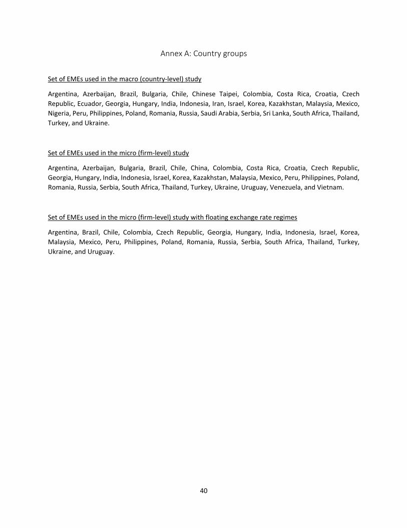
https://www.bis.org/publ/qtrpdf/r_qt1006g.htm

https://www.bis.org/publ/qtrpdf/r_qt1006g.htm

40

Annex A: Country groups

Set of EMEs used in the macro (country-level) study

Argentina, Azerbaijan, Brazil, Bulgaria, Chile, Chinese Taipei, Colombia, Costa Rica, Croatia, Czech Republic, Ecuador, Georgia, Hungary, India, Indonesia, Iran, Israel, Korea, Kazakhstan, Malaysia, Mexico, Nigeria, Peru, Philippines, Poland, Romania, Russia, Saudi Arabia, Serbia, Sri Lanka, South Africa, Thailand, Turkey, and Ukraine.

Set of EMEs used in the micro (firm-level) study

Argentina, Azerbaijan, Bulgaria, Brazil, Chile, China, Colombia, Costa Rica, Croatia, Czech Republic, Georgia, Hungary, India, Indonesia, Israel, Korea, Kazakhstan, Malaysia, Mexico, Peru, Philippines, Poland, Romania, Russia, Serbia, South Africa, Thailand, Turkey, Ukraine, Uruguay, Venezuela, and Vietnam.

Set of EMEs used in the micro (firm-level) study with floating exchange rate regimes

Argentina, Brazil, Chile, Colombia, Czech Republic, Georgia, Hungary, India, Indonesia, Israel, Korea, Malaysia, Mexico, Peru, Philippines, Poland, Romania, Russia, Serbia, South Africa, Thailand, Turkey, Ukraine, and Uruguay.

41

Previous volumes in this series

No Title Author

694 January 2018

Exchange Rates and the Working Capital Channel of Trade Fluctuations

Valentina Bruno, Se-Jik Kim and Hyun Song Shin

693 January 2018

Family first? Nepotism and corporate investment

Gianpaolo Parise, Fabrizio Leone and Carlo Sommavilla

692 January 2018

Central Bank Forward Guidance and the Signal Value of Market Prices

Stephen Morris and Hyun Song Shin

691 January 2018

Effectiveness of unconventional monetary policies in a low interest rate environment

Andrew Filardo and Jouchi Nakajima

690 January 2018

Nonlinear State and Shock Dependence of Exchange Rate Pass-through on Prices

Hernán Rincón-Castro and Norberto Rodríguez-Niño

689 January 2018

Estimating unknown arbitrage costs: evidence from a three-regime threshold vector error correction model

Kristyna Ters and Jörg Urban

688 January 2018

Global Factors and Trend Inflation Gunes Kamber and Benjamin Wong

687 January 2018

Searching for Yield Abroad: Risk-Taking through Foreign Investment in U.S. Bonds

John Ammer, Stijn Claessens, Alexandra Tabova and Caleb Wroblewski

686 January 2018

Determinants of bank profitability in emerging markets

Emanuel Kohlscheen, Andrés Murcia Pabón and Julieta Contreras

685 December 2017

Why so low for so long? A long-term view of real interest rates

Claudio Borio, Piti Disyatat, Mikael Juselius and Phurichai Rungcharoenkitkul

684 December 2017

Triffin: dilemma or myth? Michael D Bordo and Robert N McCauley

All volumes are available on our website www.bis.org.

http://www.bis.org/

BIS Working Papers · Hyun Song Shin Monetary and Economic Department January 2018 JEL...

Documents

Transcript of BIS Working Papers · Hyun Song Shin Monetary and Economic Department January 2018 JEL...