BIS Working Papers · funds of funds, macro funds, equity funds, etc) yields time-varying estimates...

BIS Working Papers No 260

Estimating hedge fund leverage by Patrick McGuire and Kostas Tsatsaronis

Monetary and Economic Department September 2008

JEL classification: G20, G23 Keywords: hedge funds, systemic risk, leverage, style analysis.

BIS Working Papers are written by members of the Monetary and Economic Department of the Bank for International Settlements, and from time to time by other economists, and are published by the Bank. The views expressed in them are those of their authors and not necessarily the views of the BIS.

Copies of publications are available from:

Bank for International Settlements Press & Communications CH-4002 Basel, Switzerland E-mail: [email protected]

Fax: +41 61 280 9100 and +41 61 280 8100

This publication is available on the BIS website (www.bis.org).

© Bank for International Settlements 2008. All rights reserved. Limited extracts may be reproduced

or translated provided the source is stated.

ISSN 1020-0959 (print)

ISSN 1682-7678 (online)

ii

mailto:[email protected]

http://www.bis.org/

Abstract

Hedge funds are major players in the international financial system and nimble investment strategies including the use of leverage allow them to build up large positions. Yet the monitoring of systemic risks posed by the build-up of leverage is hampered by incomplete information on hedge funds’ balance sheet positions. This paper describes how an extension of “regression-based style analysis” and publicly available data on fund returns yield an indicator of the average amount of funding leverage used by hedge funds. The approach can take into account non-linear exposures through the use of synthetic option returns as possible risk factors. The resulting estimates of leverage are generally plausible for several hedge fund families, in particular those whose returns are well captured by the risk factors used in the estimation. In the absence of more detailed information on hedge fund investments, these estimates can serve as a tool for macro-prudential surveillance of financial system stability.

Keywords: hedge funds, systemic risk, leverage, style analysis.

JEL Classifications: G20, G23.

iii

Contents

Abstract ................................................................................................................................................... iii Contents ...................................................................................................................................................v 1. Introduction ....................................................................................................................................1 2. Methodology and data....................................................................................................................3

2.1 Investment style analysis and leverage...............................................................................3 2.2 Estimation ............................................................................................................................6 2.3. Hedge fund data ..................................................................................................................8

3. Investment style analysis results ...................................................................................................9 3.1 Baseline estimates.............................................................................................................10 3.2 Including synthetic options factors.....................................................................................11 3.3 Assessment: does the indicator make sense? ..................................................................12

4. Concluding remarks .....................................................................................................................13 References .............................................................................................................................................15 Appendix 1: Deriving a measure of leverage .........................................................................................17 Appendix 2: Results for balanced panels...............................................................................................18 Appendix 3: Hedge funds’ exposures ....................................................................................................19

v

Estimating hedge fund leverage1

Patrick McGuire2 and Kostas Tsatsaronis3

1. Introduction

Periods of financial sector distress have often been linked to excessive levels of leverage. Thus, monitoring the aggregate use of leverage as well as its distribution across key financial sector players is a key part of an effective assessment of systemic vulnerabilities.

Leverage also plays a central role in hedge funds’ investment strategies. They can be active in a wide array of financial markets, combining long and short positions with leverage. This investment profile makes them, on the one hand, key suppliers of risk and arbitrage capital and, hence, positive contributors to market efficiency. On the other hand, their use of leverage can become a source of systemic risk if it reaches excessive levels. Crisis episodes, such as the one that followed the Russian default and the subsequent the implosion of LTCM in the autumn of 1998, highlight the possible role of hedge fund leverage in the propagation of stresses across the financial system (CGFS (1999)).

Weak formal reporting requirements for hedge funds complicate the monitoring of their use of leverage. Hedge funds are typically not required to disclose their portfolio positions to supervisory authorities and any reporting requirements provide a rather cursory and incomplete description of the funds’ overall risk profile. In the context of their normal business relationships, hedge fund counterparties, such as prime brokers, may receive risk profile information on a bilateral basis. This information is used for internal risk management and is typically not communicated externally (not even on an aggregate basis). Prudential monitoring of systemic vulnerabilities is typically based on information on size and returns that the funds report voluntarily to data vendors for the purpose of attracting business from investors, advisors and asset managers.

The purpose of this paper is to ask what can be learned about hedge funds’ use of leverage on the basis of publicly available data. In this respect, the paper belongs to a growing body of work that investigates hedge funds from the perspective of financial stability.4 The primary empirical tool is “regression-based style analysis”, a technique used to uncover the risk factors that drive portfolio returns. A rolling application of this technique across groups of funds with similar investment styles (eg funds of funds, macro funds, equity funds, etc) yields time-varying estimates of funds’ sensitivity of returns to different risk factors.5 The indicator of leverage is meant to capture the notion that gearing of the balance sheet essentially results in an amplification of the sensitivity of the hedge funds’ profit and loss to these risk factors. The proposed indicator is thus based on a natural reinterpretation of the sum of the coefficients in the standard style analysis regressions as measuring the degree of sensitivity of hedge fund performance to the risks it is exposed.

The most important aspects of the leverage indicator are its simplicity and its reliance on publicly available information. It does exploit to a fuller degree this information and it is a tool that can be readily applied for the analysis of aggregate financial market conditions. It is, however, a rather crude measure. It is based on the average sensitivity of hedge fund returns to broad asset price indices and

1 The authors would like to thank without implication Claudio Borio for extensive discussions and Nikola Tarashev for a helpful

tip. Dimitris Karampatos, Emir Emiray and Sansau Fung provided excellent research assistance. The views expressed in this paper are the authors’ own and do not necessarily reflect those of the Bank for International Settlements.

2 Monetary and Economic department, [email protected], + 41 61 280 8921. 3 Monetary and Economic Department, [email protected], +41 61 280 8082 4 Other examples include Chan et al. (2006), Garbaravicius and Dierick (2005) and ECB (2005), Gupta and Liang (2004),

Getmansky, Lo and Makarov (2004), Getmansky, Lo and Mei (2004), Adrian (2007) and Kambhu, Schuermann and Stiroh (2007).

5 Ennis and Sebastian (2003) conduct a similar analysis using an index of fund of funds returns. See also IMF (2004) for an analysis of hedge funds’ risk exposures during emerging market currency crises.

Estimating hedge fund leverage McGuire-Tsatsaronis 1

mailto:[email protected]

it relies on the assumption that funds in the same investment family tend to behave similarly. It is also quite difficult to validate, since there are no known benchmarks against which it can be compared. Nevertheless, the indicator does exhibit historical patterns that are consistent with received ideas about the level of leverage among hedge funds associated with anecdotal evidence. From this perspective, it is a useful tool for policy makers as a complement to other, less systematic sources of information, such as market intelligence and reports.

In addition to constructing this leverage indicator, the paper makes a number of other contributions to the literature that employs regression based style analysis of hedge funds. While many empirical studies of hedge fund returns rely primarily on return indices for each fund style family, this paper uses panel estimation techniques which pool information across individual hedge funds in the same fund family. This yields more robust estimates of the overall exposures for the typical (representative) fund following the particular investment style. Moreover, the use of the cross-sectional information facilitates the estimation of time-varying estimates of return sensitivity and leverage, as one can apply rolling estimation to samples of reduced length without substantial costs in terms of the degrees of freedom for the estimation. This is a distinct advantage of a panel technique over those that rely on hedge fund return indices.

Another innovation of this paper relates to the more extensive use of option-like returns as part of the risk factors that explain hedge fund portfolio returns. Hedge funds are known as nimble investors who employ on complex strategies involving derivatives in their effort to exploit investment opportunities. This suggests that, statistically, style analysis regressions that rely exclusively on benchmark index returns (such as the SP500) suffer from an attenuation (omitted variable) bias. This is because the risk factors are generally constrained to enter the regression equation linearly, even though hedge funds’ actual exposures, and hence the relationship between their performance and the returns on underlying asset classes, can be highly non-linear vis-à-vis the underlying broad market indices. For this reason, the style regressions in this paper include the returns on put and call options on many of the benchmark asset price indices used in the analysis. The use of assets with non-linear payoffs has been introduced in the literature by Fung and Hsieh (2001) as well as Agarwal and Naik (2004). This paper broadens this approach by introducing synthetically constructed returns for at-the-money put and call options on a larger number of asset classes.

The inclusion of these synthetic options increases the explanatory power of the model, and (generally) leads to higher estimates of leverage, although the results differ across fund families. For some (eg funds of funds, equity hedge and macro fund families), leverage is consistently higher when these variables are included, generally falling between two and six times assets under management (AUM). Estimated leverage for managed futures is even higher, usually in the 4-10 range. However, the estimates for these fund families also tend to be more volatile relative to the baseline model, even when estimated over relatively long (36 month) regression windows. While such volatility is consistent with changes in investment strategies over time, it also may be related to a problem of multicollinearity, which is introduced when the synthetic options factors are included in the model.6 Partially correcting for this by stripping out the independent sources of variation indicates that the synthetic options factors do contain important sources information independent of the movements in the underlying reference security. For other fund families (fixed income and relative value arbitrage, for example) the estimates of leverage are implausibly low even when the synthetic options factors are included. For these families, the set of risk factors in the regression explain considerably less of the overall variation in hedge fund returns, suggesting that further refinements in the empirical implementation are necessary to capture the idiosyncratic aspects of their investment strategies.

The rest of the paper is organised as follows. The next section lays out the style analysis regression methodology, develops the indicator of leverage, and discusses the empirical complications that arise in the estimation. Section 3 presents the style analysis results for nine fund families, and the results of a simple exercise designed to verify whether this indicator captures leverage-related movements in the data. Section 4 follows with concluding remarks.

6 Near multicollinearity in the RHS variables can lead to large swings in parameter estimates across model specifications,

particularly if there is specification error. See Winship (1999).

2 Estimating hedge fund leverage_McGuire-Tsatsaronis

2. Methodology and data

Tracking the sensitivity of hedge funds’ returns to the returns in various asset markets can help to identify broad changes in their investment strategies. The principal empirical tool is “regression-based style analysis”, a technique first applied by Sharpe (1992) to the analysis of mutual fund strategies. It involves the use of a linear regression that attributes portfolio returns (the independent variable) to a series of “risk factors” (which are the set of explanatory variables). These risk factors are typically proxied by the returns on asset classes to which the portfolio is thought to be exposed. The resulting regression coefficients measure the sensitivity of portfolio returns to changes in the returns on the underlying factors.

However, the characteristics of the hedge fund business model (compared to those for mutual funds) present some empirical complications. As Stultz (2007) succinctly put it: “[h]edge funds exist because mutual funds do not deliver complex investment strategies”. In particular, hedge funds tend to alter their portfolio exposures more frequently than mutual funds, can take larger short positions and do make more extensive use of strategies with payoffs that are not linearly related to the market risk factors. Various modifications to the basic empirical technique that have been suggested in the literature can address, to some extent, these complications.7 We propose an extension of the technique that can yield a proxy for the degree of leverage employed by the funds, which builds on this literature by exploiting the notion that leverage acts as an amplifier to the estimated sensitivity of fund returns to the underlying risk factors. The next sub-section outlines the regression-based style analysis as used here and presents the construction of leverage indicator in general terms. Section 2.2 deals with the details of estimation as applied in this paper, while section 2.3 describes the data.

2.1 Investment style analysis and leverage

The basic rationale behind the technique of style analysis can be illustrated by reference to a portfolio with allocations to k assets. The overall portfolio return can be written as the weighted average of the returns on the individual assets, with the weights being the share of total funds invested in each asset:

ktktt

HFt RwRwRwR +++= K2

11

1 (1)

If the portfolio is fully invested, the sum of the portfolio shares should be equal to 100%, or .

Moreover, if the portfolio contains only long positions, the weights should also be positive. If an analyst who observes also knows the identity of the k asset types, the weights can be recovered by solving a linear programming problem subject to the associated constraints. However, the analyst typically does not know the exact set of securities in the portfolio. Thus, estimates of the portfolio weights can be obtained using regressions which use (as explanatory variables) returns on broad market indices which are thought to resemble the asset classes that are included in the portfolio. Such regressions are often based on returns in excess of the risk free rate ( ) and the regression coefficients are then interpreted as exposures of the portfolio to these market risk factors.

1≡∑i

jw

HFtR

tr

( ) ( ) ttkt

k

kt

HFt rRrR ε+−β+α=− ∑ (2)

The specification used here includes a constant, α, and an error term, ε. The constant is meant to capture the fund manager’s skill in achieving superior returns relative to more passive portfolio strategies (in the sense of Jensen’s alpha). The error term captures (idiosyncratic) measurement error that arises from relying on broad market indices as opposed to the returns on particular securities, and from the fact that the specification can at best approximate, rather than replicate, the investment strategy of the unobserved portfolio.

7 Examples include Fung and Hsieh (2001), Brown et al (2002), Agarwal and Naik (2004) and Brunnermeier and Nagel

(2004).


The approach outlined above abstracts from the fact that the portfolio strategy might involve the use of a certain degree of leverage.

Leverage can be thought of, broadly, as increasing the sensitivity of portfolio returns to underlying risk factors. In practice, a hedge fund can achieve leverage in two complementary ways. The first, which we label funding leverage, involves outright borrowing. Taking on debt boosts the potential return to the investors in the fund because returns are earned on a portfolio of assets that is larger than the funds they contributed (assets under management, or AUM). Debt, however, gives rise to the possibility that an adverse shock to the fund’s portfolio returns might lead to negative net worth. Another reason why portfolio returns can be amplified when compared to the returns on underlying asset classes is through the choice of investment instruments, such as derivatives and structured notes. Leverage of this type, labeled instrument leverage, can amplify return sensitivity by creating exposures to underlying assets that are much higher than the original cash outlays.

The discussion which follows broadens the specification to the case where a hedge fund employs leverage, and proposes an indicator of leverage based on the coefficients which are estimated using style analysis. This indicator gauges the sensitivity of hedge funds’ portfolio returns to the returns on underlying asset classes. While simple in theory, the sophistication of hedge funds’ actual investment strategies, and the inability to decompose their returns into identifiable risk factors, complicates both the estimation and interpretation of this indicator. These issues are discussed below, and estimates of the indicator based on a variety of scenarios are presented in later sections.

To fix ideas, suppose that the risk-free rate is zero and consider the case of a hedge fund with initial AUM of £10. Suppose further that the hedge fund levers up AUM ten times by borrowing £90 to finance the purchase of a security for £100. If the value of the security at the end of the period moves to £105, the return on AUM is 50%. The fund can obtain an equivalent exposure by placing the AUM of £10 as initial margin for a long exposure to the same securitiy worth £100 through futures contracts. The return on AUM would again be 50% if the price of the security moves to £105 by the end of the period. In this simple example, the price of the reference security and the price of the derivative (eg the futures contract) move in lockstep. That is, they are related linearly.

More generally, however, movements in the prices of derivatives are related in a non-linear way to movements in the price of the underlying reference assets. For example, a 5% increase in the price of the reference security can yield a much larger (or smaller) percentage increase in the value of an option position on that security, depending on the type of the option (put or call), the position taken (long or short) and the distance between the current price of the underlying and the strike price of the option. Combinations of option positions, and, for that matter, any other dynamic multi-asset investment strategy beyond a “long-only buy-and-hold” strategy, can introduce a degree of non-linearity into hedge fund returns when these returns are dissected via style analysis using broad market indices.

It is convenient to begin by focusing exclusively on estimating funding leverage. The indicator of leverage developed here can be viewed as a reinterpretation of the estimated coefficients from equation (2). Whereas equation (1) describes the returns of a portfolio of assets with long positions in (only) spot instruments and with no debt (ie no leverage), hedge funds more closely resemble a leveraged portfolio (ie including debt) which is invested in a wide range of assets. Debt, denoted by

, can be expressed as a net short position in cash (the riskless asset), and as a multiple of the total funds contributed by investors (AUM). That is,

0≤tB 0≤θFt

tFtt AUMB *θ= .

As shown in Appendix 1, the excess returns (over the risk free rate) to investors in this hedge fund in period t, denoted by , can be written as a simple weighted average of the excess returns on

the individual non-cash assets in the portfolio, , scaled up by a leverage parameter , , as in equation (3).

tHFt rR −

tit rR − tρ

∑ −ωρ≡−i

tit

ittt

HFt rRrR )( , (3)

where and . The weight on each non-cash asset ( ) 11 ≥θ−≡ρ Ftt 1≡ω∑

i

iit i in period t , , is the

share of total funds (investors’ AUM plus debt) invested in (non-cash) asset

itω

i , and is thus different


than the w in equation (1). The leverage parameter tρ captures the overall degree to which the excess returns on non-cash assets are amplified by the short position in cash. Since the sum of the weights on the excess returns on non-cash assets equals unity, then an estimate of the leverage parameter, , can be obtained simply by summing the estimated coefficients in an empirical equation such as (2). That is, given estimates of β from a regression of equation (2) for a particular time period

,

tρ

t

tti

it

kkt ρ=ρω=β ∑∑ ˆˆˆ (4)

The level of ρ can be interpreted as the ratio of the total size of the fund’s asset portfolio to its AUM. For example, a value of one would imply no leverage, while a value of two would imply portfolio positions (assets or exposures) that are twice as large as the investors’ capital with the fund (AUM).

ˆ

The accuracy of this empirical technique in gauging the degree of funding leverage depends on whether the actual positions of the funds can be identified. While the explanatory variables typically used in style analysis regressions are excess returns on broad market indices, hedge funds regularly take positions in derivative instruments where the reference asset could be a specific security or a market index. Moreover, derivative-style payoffs can be generated synthetically through complex trading strategies, which may combine both outright and derivative positions in a particular asset with debt and shorting strategies.

Failure to include the returns on such positions (or to adequately proxy for them) as regressors introduces important sources of error in the estimation. First, there is an approximation error arising from the fact that portfolio returns are non-linear functions of the return on the underlying asset classes while the estimated model is linear in those returns (equation 1). The second problem arises from the fact that there are omitted variables in the estimated model leading to an attenuation bias which corrupts the coefficient estimates and hence the indicator of funding leverage.

To understand the omitted variable bias, consider the example of a hedge fund which borrows to finance an outright position in the S&P 500, as well as to put up margin for derivative positions (a put and a call) with the S&P 500 index as the reference security. Let be the return on the outright

position, and and be the returns on long positions in specific put and call derivative contracts. Using equation (3), the excess return on this total portfolio position would be

SPtR

ctR p

tR

( ) ( ) ( ) ( )[ ]tpt

pt

ct

ct

SPt

SPt

HFt rRrRrRrR −ω+−ω+−ωρ=− ,

where the weights and the leverage parameter are defined as above. An econometrician armed with the return series for the reference asset and the for the derivative contracts can obtain an unbiased estimate of funding leverage, ρ , by estimating

( ) ( ) ( ) ( ) ttpt

pt

ct

ct

SPt

SPt

HFt rRrRrRrR ε+−β+−β+−β=−

and then summing the estimated coefficients as prescribed by equation (4).

Now suppose that the returns on the put and call option are not included as regressors. This would result in biased estimates of leverage because (a) they are potentially important variables which are not being included in the sum in equation (4) and (b) the coefficient estimates on those regressor variables which are included, in this example, may be biased. Specifically, a regression of

on only would yield a coefficient on this regressor of

SPβ

( tHFt rR − ) )( t

SPt rR −

SP

tSPt

tSPtt

ptp

tSPt

tSPtt

ctcSPSP

rRrRrR

rRrRrR

β≠⎥⎦

⎤⎢⎣

⎡

−−−

β+⎥⎦

⎤⎢⎣

⎡

−−−

β+β=β)var(

),cov()var(

),cov(~ (5)

The direction of the bias, captured by the second and third terms in equation (5), depends on whether the portfolio is long or short in the particular derivatives contracts, and on the strength of the correlation between the returns on the reference security and the derivatives positions.

Typically the return on an option contract is very highly correlated with the return on the reference security. The correlation is positive in the case of calls and negative in the case of puts. Thus, for


example, if a hedge fund has a long position in the reference S&P 500 index ( ) and a long

position in the call contract ( ), would be biased upwards since the covariance between the call and the reference index is positive. A similar argument applies to a short position in the put ( ), since the covariance between the returns on the put and the reference index is negative. On balance, since the actual long and short positions are unknown it is impossible to know whether an estimate of leverage is biased upwards or downwards in a regression which includes only broad market indices.

0>βSP

0>βc SPβ~

0<β p

The empirical problems which arise in this context can in part be mitigated by the inclusion of regressors which capture these non-linearities. Fung and Hsieh (2001) and Agarwal and Naik (2004), working with hedge fund return indices at the fund family level, adopted this approach and showed that the inclusion of derivative-like returns as explanatory variables can improve the estimation results in standard style analysis regressions. The next section outlines an estimation strategy which can handle a large number of regressors, and which attempts to take into account hedge funds’ non-linear exposures.

Even when derivative and other complex financial instruments are explicitly included as regressors, the estimated coefficients do not necessarily yield a clean estimate of funding leverage (as distinct from instrument leverage). For example, the returns on futures and forwards are linear in the price of the underlying reference security, yet these instruments represent a type of instrument leverage. These positions are empirically indistinguishable from a leveraged long position in the security (funding leverage). Thus, while the inclusion of non-linear variables certainly can help in generating better estimates of funding leverage, these estimates will, in addition, reflect all instrument leverage which generates linear exposures to the broad market indices.

2.2 Estimation

Equations (3) and (4) present a tradeoff of sorts. A time-invariant estimate of funding leverage could be calculated separately for each hedge fund. This approach sheds light on the behaviour of a individual hedge funds, but would require a long time-series of fund returns or restrictions on the number of RHS regressors used to estimate leverage. Alternatively, estimates of average leverage for shorter time periods and based on much larger sets of RHS risk factors can be generated by exploiting the cross-sectional dimension in a panel of hedge fund returns. A rolling application of this second technique can potentially capture broad shifts in investment strategy, as hedge funds respond to changing market conditions.

This paper adopts this second approach. The estimation of time-varying sensitivity parameters (β’s) is carried out using rolling regressions on panels of monthly returns for hedge funds in nine fund families across the January 1996 – June 2007 time period.8 The nine fund families are based on the classification by HFR and discussed in greater detail in the data sub-section below.

Within each regression window, estimation is performed in two stages. The first stage relates to the selection of the RHS risk factors that best explain the portfolio returns within the specific window, and the second stage yields the actual estimates of the betas used to calculate leverage. The procedure has been devised so as to minimize the impact from spurious relationships on the estimated portfolio exposures and leverage. The identification of those risk factors most relevant for the specific investment style and in the specific period window is performed by means of a stepwise regression of hedge funds’ excess monthly returns on the full set of risk factors. The stepwise procedure recursively adds and drops RHS risk factors, and retains them only if their statistical significance exceeds a certain threshold.9

8 The nine investment style families are: funds of funds (FOF), equity hedge (EQHED), equity no-hedge (EQNOHED), event driven (EVNTDRV), macro (MACRO), market neutral (MKTNEUT), managed futures (MNFUT), relative value arbitrage (RVALARB) and fixed income (FXINC).

9 The stepwise regression requires that there be at least as many months in the regression window as there are right-hand side variables. Since we experiment with a large number of market risk factors, the window lengths are generally quite long, usually 24-36 months, depending on the model specification. The tolerances for inclusion and exclusion of RHS variables in the stepwise procedure are set at p-values of 0.05. and 0.06, respectively, although similar results emerge if the parameters


The second stage applies a fixed-effects regression of hedge fund returns on the set of factors identified in the first stage. The coefficient estimates from this second stage regression are used in calculating leverage for the particular fund family and regression window. Since short positions would appear as a negative estimated coefficient, the indicator of leverage is the sum of the absolute value of the estimated coefficients.

The “investable universe” is taken as a set of 31 market risk factors that cover various types of risk. These factors cover the US and international equity markets, the US government and corporate bond markets, specific credit risk factors, gold, and returns on currency carry trades, and are generally similar to those used in other studies. Table 1 lists the full set of right-hand-side (RHS) variables, and Graph 1 plots the time series returns for a few of the major indices.

As discussed above, hedge funds make extensive use of derivatives and other instruments and strategies which lead to highly non-linear exposures to these broad market risk factors. As a result, estimation of equation 3 using only the the broad market risk factors will yield biased coefficient estimates. However, including the returns on option-like strategies as RHS risk factors can help to correct for omitted factors (Fung and Hsieh (2001), Agarwal and Naik (2004)). The approach adopted here is to generate synthetic one-month returns on hypothetical options contracts by backing out estimates of the price of such contracts from the Black-Scholes formula. The only unknown parameter in this setting is expected volatility, is proxied by the historical volatility calculated from daily observations. Thus, the inclusion of these synthetic option factors as RHS variables can be thought of as including historical volatility in the linear regression model, but in a particular (non-linear) way.

For each of seven market risk factors – the MSCI World ex US equity index (MSCIWxUS), S&P 500 index (S&P500), MSCI emerging market equity index (MSCIEM), Solomon Brothers World government bond index (SBWGBI), Lehman Brothers high yield CCC index (LBHYCCC), Goldman Sachs commodity index (GSCOM), gold price (GOLD), and JPMorgan’s global emerging market bond index (EMBIG) – the two month and three month at-the-month (ATM) synthetic option prices (for both puts and calls) are calculated using a Black-Scholes option pricing model.10 These estimated prices yield a set of synthetic returns, corresponding to a hypothetical strategy of purchasing an ATM contract (either a put or call) on the underlying reference index and then selling it one month later, which are then incorporated as additional risk factors in the first stage step-wise regression.11

The high correlation between the synthesized returns on put and call options and the actual returns on the reference index, evident in Graph 1 presents an empirical problem. In the classical framework, “near multicollinearity” does not bias the coefficient estimates, but it does increase the estimated standard errors of the estimates. With higher standard errors, some RHS risk factors may inadvertently be dropped in the first stage stepwise regression described above, since this procedure retains only those risk factors which are significant beyond a certain threshold. To deal with this issue, the returns on the synthetic options factors are first orthogonalized by regressing them on the corresponding reference index. The residuals from this regression, which contain the variation in the synthetic option returns independent of the variation in the reference index, are used in selecting the appropriate set of risk factors in the first-stage stepwise regression. Once the appropriate set of risk factors has been identified, the original (ie non-orthogonalized) versions of the synthetic option factors are included in the second stage fixed-effects regression.

There are several other adjustments that are made in order to improve the fit of the model. Within each regression window, those funds which report a return greater than the 99th percentile or less than the 1st percentile (within each regression window) are excluded. In addition, hedge funds which have

are relaxed to 0.20 and 0.21. Note that this procedure used in this paper differs from the that in McGuire et al. (2005). In the latter, the first stage regression relied on data across the entire sample period, and the set of right hand side variables was then held fixed in individual regression windows.

10 To get an estimate of the expected volatility, an asymmetric GARCH model is fitted to the daily spot price of returns for various market indices. The GARCH parameters are then used to simulate volatilities (500 simulations), and the average of the these is taken as the input for the Black-Scholes option pricing formula. This calculation is performed separately for maturities of 2 and 3 months, although only the monthly returns based on the two month maturity are used in the analysis.

11 Applying this procedure to the S&P 500 index, where actual data on options prices are available for some periods (and was used in Agarwal and Naik (2004) and McGuire et al. (2005)), yields synthetic options returns that are very similar to the option returns calculated with actual price date; the correlation between the actual and the estimated prices exceed .93 for both put and call prices.


fewer than 14 months of data within a particular window are dropped. While these modifications lead to slightly different samples of hedge funds being used across regression windows, it generally improves the fit of the model and smoothes the coefficient estimates on particular RHS regressors without materially affecting the overall results.12

2.3. Hedge fund data

Hedge funds do not face the same disclosure requirements as other investment vehicles available to the retail investor, such as mutual funds. As a result, the main source of information on hedge funds is a small number of commercially available databases containing data which are voluntarily provided by the funds, presumably to publicise their track record and to attract additional capital. In most cases, there is little or no information on portfolio allocation, or comprehensive measures of risk and leverage. The analysis in this paper relies on a dataset compiled by Hedge Funds Research (HFR), which includes information on hedge funds’ monthly returns (net of fees) and assets under management (AUM).

The fact that hedge funds voluntarily disclose data gives rise to several biases that can cloud the interpretation of empirical analyses. For example, HFR provides monthly data instalments which include historical performance for those funds which chose to report to HFR during the month. Funds that stop reporting at some point in time are dropped in subsequent monthly instalments, thus introducing a survivorship bias.13 To minimize this bias, the monthly instalments have been merged over the December 2001–June 2007 period. This preserves the information about all funds that were included in at least one HFR monthly instalment during this period, but clearly does not distinguish between the various potential reasons for fund disappearance.14 Funds which report to HFR for the first time in a given month often include a history of their returns and AUM. Thus, the history of the compiled database (eg overall average returns, total number of funds, etc) can change each time a new month of data is added, depending on how many new funds report and how complete their historical time series of returns is. This, in turn, implies that the estimates of (historical) leverage, such as those presented below, below will evolve as the database is updated from month to month.

Graph 2 presents some figures for the number of hedge funds reporting data to HFR. The top panels are based on the number of unique hedge fund names in each monthly update of the HFR data, broken down by the location of office and the legal domicile. The analysis is based on the union of all monthly files collected since Dec 2001. In the most recent file (June 2007), roughly 7000 funds reported data, most of them funds managed out of London, Switzerland, New York or elsewhere in the United States (top left-hand panel). The majority of these are structured as financial entities legally domiciled in the Caribbean offshore centres (particularly those funds managed in London) or in the United States, primarily in Delaware (Graph 2, top right-hand panel).

Not all funds which report to HFR in a given month provide the complete history of their returns. In fact, roughly one-quarter of the funds identified in any given monthly update from HFR do not provide data for returns for the 3-5 months prior to the reporting date, even though they do provide return data for the more distant past. The bottom panels of Graph 2 provide the number of funds for which there is non-missing data on monthly returns, broken down by fund family. These fund families, defined by HFR, are constructed on the basis of reporting funds’ self-described investment strategy.15 The hump

12 The overall level and time variation of leverage changes little when the full sample is used, although the volatility of the

estimates increases relative to those based on the restricted sample. 13 Databases can also suffer from sample selection bias, since hedge funds may report to only one database vendor, implying

that no one database provides a comprehensive picture of the industry. Agarwal et al (2004) compile the databases from three different commercial providers and find only a 10% overlap. In addition, hedge funds that do report may so only after a period of strong performance, leading to an “instant history bias” which tends to overstate funds’ average experience, and hence the average performance in the database. See Fung and Hsieh (2000, 2002b) for more discussion.

14 Poor performance (or outright closure) is a frequent cause for a cessation in reporting, implying that the database would tend to flatter the overall performance of the industry. Conversely, larger funds may decide to close to new investors and thus cease reporting. This could bias downwards the performance information in the database if funds tend to close to new investors after a sustained period of good performance that attracts more AUM than can be profitably invested.

15 The fixed income (FXINC) style family is based on five underlying families defined by HFR: FIXINC_ARB FIXINC_CONV FIXINC_DIV FIXINC_HI and FIXINC_MORT.


in the number of funds (total) evident in these graphs reflects the fact that many funds report their results but only with a lag of 2-4 months. Funds-of-funds and equity no-hedge hedge funds are by far the most numerous in the HFR database, although the number of funds in other fund families has been growing (Graph 2, bottom left- and right-hand panels).

Hedge funds, overall, have performed relatively well throughout the Jan 1996-June 2007 period, although there have been bouts of low returns and high volatility. Many fund types managed to generate consistently positive average returns, at least when measured using a 36 month rolling window.16 The average returns generated by equity market related strategies tended to fluctuate between the upper or the lower extremes of the performance range (Graph 3, top panel), while the returns to other strategies were more concentrated in the middle (Graph 3, top right-hand panel). Moreover, the returns for several fund families which supposedly have unique investment strategies are strikingly similar, suggesting a significant degree of commonality in their exposures. For example, the average returns to equity hedge and equity no-hedge funds have a correlation of 0.73, while the correlation between those of funds-of-funds and these two equity related strategies was even higher, at 0.83 and 0.97 respectively. Similarly, macro funds and managed futures funds (0.86), and macro funds and relative value arbitrage funds (0.63), also co-move to a considerable degree (Graph 3, top right-hand panel).

Similarities across fund families are apparent when one looks at the volatility of performance as well. The lower panels of Graph 3 plots the simple average (across funds) of the fund-specific 36-month rolling standard deviation of returns for each of the fund families. Between 2000 and 2007 the average volatility for most fund families has been drifting downwards, with the possible exception of funds-of-funds and relative value arbitrage (RVALARB) funds, both of which already exhibited volatility at the lower end of the range. Moreover, the difference (across fund families) between the highest and lowest average volatility decreased considerably during this period from about 0.6 to about 0.3. This convergence in performance is generally consistent with anecdotal reports that the growth of the industry has led to greater “institutionalization” of the hedge fund sector. Hedge funds competing for investments from pension funds and other institutional investors have been increasingly forced to adopt more stable investment profiles, and aim to deliver more predictable returns, even at the expense of the absolute level of those returns.

3. Investment style analysis results

In this section, the style analysis regression model described by equation (2) is estimated separately for each of the nine fund families. Five estimates of leverage are generated, each of which is based on a slightly different empirical specification. All regressions are based on a 36 month regression window, where the RHS variables are subsets of those listed in Table 1. The estimation results are presented below (and in the appendixes) in some detail, and the empirical issues that arise are discussed along the way.

The five estimates of leverage are generated using different empirical specifications within the regression windows. The simplest measure, LEV1, is based on a single-stage fixed effects model, taking all “non-option” factors as RHS variables. LEV2 is the same as LEV1, but includes the synthetic options factors as RHS variables. For these two estimates, no step-wise search procedure is performed, and only those coefficients which have a t-statistic greater than or equal to 1.59 are used in calculating leverage. For ease of exposition, these estimates will only be discussed in passing. The other three measures, LEV3, LEV4 and LEV5, are based on slightly different versions of the two-stage stepwise estimation procedure described above. Analogous to LEV1 and LEV2, the synthetic options factors are excluded in LEV3 and included in LEV4. The final estimate, LEV5, will be discussed below.

16 The excess return and volatility measures in Graph 3 are based on the samples used in the regressions described in the

next section. As described above, hedge funds with returns greater than the 99th percentile and less than the 1st percentile within each 36 month rolling window have been dropped for these calculations.


3.1 Baseline estimates

The estimates of leverage for eight of the nine fund families are presented in Graphs 4-7. For each fund family, the left hand panel presents the regression R-squared and the number of hedge funds used in the second-stage fixed-effects rolling regressions for three regression models (LEV3, LEV4 and LEV5). The right-hand panel presents the three estimates of leverage and the associated 95% confidence intervals.17 Some results based on balanced panels of hedge funds are presented in Appendix 2.

The overall fit of the models depends on the fund family. For some families, in particular those four with similar return patterns shown in the top left-hand panel of Graph 3, the set of RHS variables explains a considerable amount of the variation in hedge fund returns. The goodness of fit, measured by the rolling regression R-squared, for these four fund families tends to be higher than for the other fund families, and generally seems to improve as the regression window moves forward through time. At the other end of the spectrum are fixed income funds, macro funds and market neutral funds, where the explanatory power of the set of RHS risk factors is quite limited.

Across all fund families, the RHS variables seem to work best for funds-of-funds, accounting for more than 60% of the variation in returns in the most recent regression windows. This probably reflects the fact that these funds, by definition, are diversified across many different investment styles and underlying risk factors, and thus their returns more closely resemble the broader market movements captured by the market indices used here than would the returns of an individual hedge fund with an idiosyncratic investment strategy. By investing across a number of individual hedge fund managers, funds-of-funds achieve a degree of diversification of idiosyncratic risk that is reflected in the higher systematic component that is picked up by the style regression.

The returns across most fund families seem to be heavily influenced by equity market factors. The individual coefficient estimates are presented in Appendix A3 for some risk factors and fund families, but there are a few points worth mentioning here. First, the returns on the broad equity market index (S&P500) and the associated synthetic option factors are almost always important drivers of performance. Similarly, other equity market related factors, such as the Fama-French SMB and HML factors enter significantly in most regression windows, and there are some striking similarities in the exposure patterns to these factors (in particular to the S&P 500 and the SMB factors) for funds-of-funds, event driven, equity hedge and equity-no hedge funds (Graphs A3.1-A3.3 in Appendix 3).

However, the estimates of leverage based on this baseline model (LEV3) appear to be unreasonably low for many fund families. Equation (4), taken literally, implies that an estimate of equal to one is synonymous with no funding leverage. Thus, estimated values below one suggest problems in the empirical implementation, such as omitted RHS risk factors. For example, the 95% confidence interval for the LEV3 estimate of leverage for funds-of-funds is reasonably tight (Graph 4, top right-hand panel), which is not particularly surprising since the RHS regressors are chosen in the step-wise regression procedure based on their statistical significance (and they are generally quite significant). However, the LEV3 estimate never deviates far from one, suggesting that funds-of-funds do not make use of leverage very often.

ρ̂

The results for other fund families based on the LEV3 model are even less convincing. Estimated leverage for equity hedge and equity no-hedge funds, presented in Graph 5, never deviates far from one, and in many cases is below one. In Graph 6, estimated leverage for managed futures funds is noticeably higher, at around three, but the regression fit is lower than for the other fund families, and does not appear to improve is the estimation moves forward through time. The results for macro funds (Graph 6) and relative value arbitrage and fixed income funds (Graph 7) are some of the least plausible across fund families; estimated leverage is often below one, and the R-squared is generally below 10%.

17 These error bands are calculated using the delta method in STATA’s “nlcom” command. They represent the 95%

confidence interval for the sum of the absolute values of the (statistically significant) underlying regression coefficients (a non-linear transformation).


3.2 Including synthetic options factors

The estimates change significantly when the synthetic options are included as possible RHS regressors. The inclusion of these factors generally improves the regression fit, at times significantly so. For example, the R-squared for funds-of-funds jumps by roughly 10 percentage points when these factors are included (Graph 4, top left-hand panel). A similar improvement is evident for event driven, managed futures and macro hedge funds (Graphs 4-6). In contrast, the addition of these variables does little to improve the fit for equity hedge and equity no-hedge hedge funds.

More importantly, the estimates of leverage (LEV4) are generally higher (but more volatile) than the LEV3 estimates. For some fund families (eg funds-of-funds, equity hedge, equity no-hedge and managed futures) the range of the estimates appears more plausible; the LEV4 estimates are more often larger than one, and rise to as high as 12. Taken at face value, the volatility of the estimates suggest that hedge funds quickly gear up and then unwind their positions. The funds-of-funds family, for example, employs, on average, leverage that is roughly two to six times their AUM, while the average level for the managed futures family is above five (Graph 6).

The estimates of leverage based on LEV4 relative to LEV3 are larger for two reasons. First, the addition of the synthetic options as RHS variables will, all else equal, increase leverage if the resulting coefficient is statistically significant, since it would then be included in the summation (equation (4)) used to compute leverage in each regression window. In general, however, this effect is quite small. The much larger contribution comes from changes in the coefficient on the reference market index. The coefficients on the RHS factors which do not have associated synthetic put and call options change little when these options are included RHS factors. This can be seen by examining the top panels of Graphs A3.1-A3.4 in Appendix 3. However, those on the RHS factors which do have associated synthetic options change significantly (Graphs A3.1-A3.3, bottom panels).

Clearly, the inclusion of the synthetic options makes a difference in the estimates of leverage. As discussed in section (2), the returns on these options are highly correlated with those on the associated reference market indices. In the classical regression framework, the estimated coefficients are not biased in the presence of multicollinearity as long is the model is well specified, that is as long as there is no residual correlation between the included RHS regressors and the error term. Indeed, the standard remedies to multicollinearity are generally offered up in discussion of the standard errors on the estimates, which can rise as the correlation between the multicollinear RHS regressors and the error term grows. In the case under consideration here, the selection of RHS regressors is based on a first-stage stepwise regression which takes the set of orthogonalized option returns as regressors. The second stage regression yields unbiased estimates of the coefficients on the original (ie unorthogonlized) regressors. Thus, there is no reason to suspect that the estimate of leverage based on LEV4 is biased. In contrast, LEV3 is likely to suffer from the omitted variable bias discussed in section (2).

However, the regression model may be mis-specified, in which case the presence of multicollinearity can be a significant problem for the level of the estimates themselves. For example, Winship (1999) demonstrates that even a relatively modest level of correlation between the error term and the RHS variables (caused, for example, by omitted factors in the error term) can lead to large swings (across model specifications) in the coefficient estimates in the presence of multicollinearity.18 While the stepwise procedure used above is designed to select the most relevant set of RHS risk factors, the set of possible risk factors from which these are drawn is far from comprehensive. The high correlation between the options and reference market indices seems to exacerbate any bias which may already be in the model, thus inducing the significant swings in estimated leverage across regression windows.

There is no easy correction to this problem. However, to better understand how much the independent information in the synthetic option returns contributes to the baseline estimate of leverage (LEV3), a final estimate, LEV5, was calculated. LEV5 is the same as LEV4, except that the fixed effects regression in the second stage is run on the orthogonalized synthetic option returns which survived the first-stage stepwise regression, rather than on the set of original unorthogonalized synthetic option returns as in LEV4. This is equivalent to including only the variation in the options returns which is

18 Winship (1999) discusses this issue in some detail, and offers up a Baysian estimation approach which incorporates both

sample uncertainty and model uncertainty in the parameter estimates.


independent of the variation in the reference market index. This eliminates the multicolinearity between these RHS variables, but at the cost of re-introducing a bias in the coefficient estimates on the reference market indices.

To see this, consider again the case of a fund exposed to the S&P 500 index and the call option on with this index as the reference security. The excess return on the call option can be decomposed into two parts by regressing it on the S&P 500 index, as in equation (6) below.

( ) ( ) ∗∗ ε+−β=− ttSPtt

ct rRrR ˆˆ (6)

Inserting the right hand side of (6) into equation (2) yields

( ) ( ) ( ) ( ) ttc

tSPt

cSPt

HFt rRrR ε+εβ+−ββ+β=− ∗∗ ˆ*ˆ

( ) ( ) ttc

tSPt

SP rR ε+εβ+−β= ∗ˆ~ (7)

Estimation of (7) would yield unbiased estimates of . However, the resulting coefficient on the S&P

500 index, ,is a function of the true beta on the index, , the true beta on the call option, , and

the estimated correlation between the call and the reference index, . In other words, is the same as the coefficient described by equation (5) in section (2). Thus, the resulting estimate of leverage based on equation (7), LEV5, is biased in the same way as LEV3. The difference in the levels between these two estimates will be a function of the importance of independent information in the options factors, ie the contribution from .

cβSPβ~ spβ cβ

∗β̂ SPβ~

cβ

The estimates of LEV5 are presented as the red lines in Graphs 4-6. A comparison of the individual coefficient estimates from LEV5 with those of LEV3 (analogous to the graphs in Appendix 3) shows that the coefficient estimates on those risk factors associated with synthetic options change little when estimated using LEV5. As a result, LEV5 is generally lower than LEV4, but higher than LEV3. Taking LEV3 as the baseline estimate, much of the increase in estimated leverage evident in LEV4 (relative to LEV3) arises from removing the attenuation bias in the estimated coefficients on the reference market indices. However, the put and call options do seem to contain important sources of independent information.

3.3 Assessment: does the indicator make sense?

By some measures, the estimates of leverage are plausible, at least for some fund families. Estimates for funds-of-funds, equity hedge, event driven and managed futures are generally bounded from below at one (or something close to one), and often fall within a range of 2-6 times AUM. These values are at least in the same ballpark as the anecdotal figures that tend to come up in conversations with market participants. However, as discussed in the previous section, the estimates are disconcertingly volatile, casting doubt on the usefulness of this indicator. Rather than tracking slow, steady buildups of leverage, the indicator, when taken literally, suggests that even the average level of leverage (across hedge funds and months in the estimation window) for a particular fund family can change suddenly, and by a large amount. This volatility in the estimates, and the relatively low regression fit for many fund families, brings up the question of whether the empirical strategy used here generates anything other than statistical noise.

Can the leverage indicator somehow be tested? There are several possible strategies. For example, establishing a link between movements in the leverage estimates and other possible indicators of hedge fund activity – eg commercial or interbank loan flows or turnover of particular financial instruments in various markets – would provide at least some evidence that the indicator captures some aspect of leverage. A full analysis of this sort is beyond the scope of this paper, but is the subject of ongoing work.

The information contained in the HFR database itself also provides the raw materials for a simple test which can potentially shed light on this issue. Many hedge funds, when they report to HFR, indicate


whether they do or do not use leverage (ie “yes” or “no”), but generally do not provide information on the extent or type of leverage employed.19 This information allows for a comparison of estimates for two groups of funds within a each fund family: those funds which reportedly use leverage (LEVY funds), and those that do not (LEVN funds). If the indicator is actually picking up greater funding leverage, and if the hedge funds which report using leverage actually do use it, then the estimate of leverage for LEVY funds should, all else equal, be higher than that for the LEVN funds.

As in the previous section, this test is conducted using 36 month regression windows on unbalanced samples of US dollar based hedge funds. This test is performed twice for each fund family, both including and excluding the synthetic options factors as RHS variables, but only the results from the no-options regression (LEV3) are presented here. Graphs 8-10 present for each fund family the average returns and volatility (left-hand panels), the regression fit and the number of hedge funds used in generating the estimates (centre panels) and an estimate of LEV3 (right-hand panels).

Across most of these samples, LEVY funds tended to have higher average returns, consistent with greater use of funding leverage, but also higher volatility than LEVN funds. The results for funds-of-funds are perhaps the most robust since the split into LEVY and LEVN funds yields large and roughly equal samples of funds, and the regression fit is similar across the two groups (Graph 8, top centre panel). A similar pattern in average returns and volatility is evident for most (but not all) other fund families as well (Graph 9).

More importantly, the estimates of leverage tend to be higher for those funds which report using leverage. Estimates of LEV3 for funds-of-funds and equity hedge funds (Graph 8, right-hand panels), are again rather low, in many cases less than one. However, in virtually all regression windows, estimated leverage for the LEVY group is higher than for the LEVN group, often usually significantly so. A similar but more pronounced pattern is evident in Graph 9 for managed futures and macro hedge funds. Estimates based on LEV4 (not presented) indicate similar cross-group patterns; the level and the volatility of the LEV4 estimates are similar to those for the full samples (Graphs 4-7), but within most fund families, LEV4 is higher for LEVY funds than for LEVN funds. In summary, the leverage indicator does seem to be picking up information related to the actual use of funding leverage, even if the resulting estimates of leverage at the fund family level are suspiciously low.

4. Concluding remarks

By relating portfolio returns to pre-specified market risk factors, style analysis is an important tool in analysis the investment strategies of hedge funds. It also serves as the basis for a simple time-varying indicator of leverage, based on the degree to which the returns on risk factors are amplified in the returns on capital held by hedge funds. This paper has explored the properties of this indicator, and presented the empirical results for nine fund families in the HFR database.

The results suggest that while there is considerable diversity in investment strategies among hedge fund families, there are also striking similarities in their risk exposures. The most qualitatively significant risk factors in this regard seem to be those that are related to the equity (in particular the US equity) market.

The ability of the leverage indicator to track actual (average) leverage depends critically on how well the RHS risk factors capture the hedge funds’ true exposures. When estimated with a limited set of market risk factors, the estimate of leverage appears to be quite low, at least relative to what anecdotal evidence would suggest. In part, these estimates seem to suffer from an attenuation inconsistency, since the broad market indices used in the baseline regression model enter linearly, while hedge funds’ actual exposures to these market risk factors are highly non-linear.

In an attempt to deal with this issue, synthetically generated returns on hypothetical options contracts were added as RHS risk factors. The overall estimated level of leverage generated using these

19 Under the HFR data field “leverage”, some typical entries include “Yes”, “No”, “Yes, but minimal”, “Yes, twice AUM”, “No (but

allowed)” etc. These unique entries were cleaned, and used to generate a bi-variate “yes” or “no” dummy variable for the purpose of sorting funds.


additional RHS risk factors appears plausible for many fund families. However, it tends to be volatile. While consistent with changes in investment tactics, the volatility may also reflect problems in the empirical implementation due to the high degree of multicollinearity introcuded by the synthetic options regressors. However, these regressors remain important explanatory variables even after stripping out the independent source of variation, highlighting the importance of acuratly capturing hedge funds non-linear investment strategies.

Overall, the results of this paper suggest that extracting reasonable estimates of hedge funds’ use of leverage from publicly available data is not a straightforward exercise, leaving room for future improvements in the empirical technique. The complexity of hedge funds’ actual positions, and the difficulty in tracking their exposures, significantly complicates any empirical application of the theory outlined in section (2). While the results presented above do suggest that the proposed indicator can pick up leverage-related movements in the data for most fund families, the differences in the quality of the estimates across families suggests that a more “style specific” set of explanatory variables may be needed. Several recent papers (eg Teiletche and Tampereau (2005)) have explored the properties of a broad set of potentially important RHS risk factors, some of which are designed to control for dynamic trading strategies and non-linear exposures, but which have not yet been tested in this setting. Another potential area for improvement is to use a more sophisticated search routine to group funds within each fund family based on the degree of commonality in their return series. Regressions based on smaller groups of funds which have similar return characteristics should yield tighter regressions, and potentially more accurate estimates of leverage.20

20 One potentially convenient approach is via principle components analysis, where funds (within a particular family) can be

grouped according to how strongly their returns load on each principle component (see Christiansen et al (2004) for a particular application of this technique). The leverage estimates for these smaller groups of funds can then be averaged (weighted by AUM), to yield broader indicators of leverage across a wider range of fund types.


References

Adrian, T (2007): “Measuring risk in the hedge fund sector”, Federal Reserve Bank of New York, Current Issues in Economics and Finance, vol 13, no 3, March/April.

Agarwal, V, N D Daniel and N Naik (2004): “Flows, performance and managerial incentives in hedge funds”, working paper presented at the Gutmann Center Symposium on Hedge Funds, University of Vienna, 29 November.

Agarwal, V and N Naik (2004): “Risks and portfolio decisions involving hedge funds”, The Review of Financial Studies, Spring, vol 17, no 1, pp 63–98.

Brown S, W Goetzmann and J Park (2002): “Hedge funds and the Asian currency crisis”, The Journal of Portfolio Management, Summer, 6(4), pp 95–101.

Brunnermeier, M K and S Nagel (2004): “Hedge funds and the technology bubble”, The Journal of Finance, vol LIX, no 5, October, pp 2013–40.

Chan, N, M Getmansky, S Haas and A Lo (2006): “Do hedge funds increase systemic risk?” Economic Review, Federal Reserve Bank of Atlanta, Fourth Quarter.

Christiansen, C, P Madsen and M Christensen (2004): “A quantative analysis of hedge fund style and performance”, Intelligent Hedge Fund Investing, ed. Barry Schachter, Risk Books

Committee on the Global Financial System (1999): A review of financial market events in autumn 1998 (“The Johnson Report”), Bank for International Settlements, http://www.bis.org/publ/cgfs12.pdf.

Ennis, M and M D Sebastian (2003): “A critical look at the case for hedge funds”, The Journal of Portfolio Management, Summer, pp 103–12.

European Central Bank (2005): “Large EU bank’s exposures to hedge funds”

Fama, E and K French (1993): “Common Risk Factors in the Returns on Stocks and Bonds”, Journal of Financial Economics, vol 33, no 1, pp 3–56.

Fung, W and D Hsieh (2000): “Performance characteristics of hedge funds and CTA funds: natural versus spurious biases”, Journal of Financial and Quantitative Analysis, 35, 291–307.

——— (2001): “The risk in hedge fund strategies: theory and evidence from trend followers”, The Review of Financial Studies, Summer, vol 14, no 2, pp 313–41.

——— (2002a): “Asset-based style factors for hedge funds”, Financial Analysts Journal, September/October, pp 16–27.

——— (2002b): “Hedge-fund benchmarks: information content and biases”, Financial Analysts Journal, January/February, pp 22–34.

Garbaravicius, T and F Dierick (2005): “Hedge funds and their implications for financial stability”, European Central Bank Occasional Paper Series, No. 34

Getmansky, M, A W Lo and I Makarov (2004): "An econometric model of serial correlation and illiquidity in hedge fund returns," Journal of Financial Economics, vol. 74, no. 3, pp. 529-609.

Getmansky, M, A W Lo, and S X Mei (2004): "Sifting through the wreckage: Lessons from recent hedge-fund liquidations," Journal of Investment Management, vol. 2, no. 4, pp. 6-38.

Gupta, A and B Liang (2005): "Do hedge funds have enough capital? A value-at-risk approach," Journal of Financial Economics, vol. 77, pp 219–253.

International Monetary Fund (2004): Global Financial Stability Report, April, pp 146–8.

Kambhu, J, T Schuermann and K Stiroh (2007): “Hedge funds, financial intermediation and systemic risk”, Economic Policy Review, Federal Reserve Bank of New York, vol 13, no 3, December.

McGuire P, E Remolona and K Tsatsaronis (2005): “Time varying exposures and leverage in hedge funds”, BIS Quarterly Review, March


http://www.bis.org/publ/cgfs12.pdf

Sharpe, W (1992): “Asset allocation: management style and performance measurement”, The Journal of Portfolio Management, winter, pp 7–19.

Stulz, R (2007): “Hedge funds: Past, present, and future”, Journal of Economic Perspectives, Vol 21, No 2, Spring.

Teiletche, J and Y Tampereau (2005): “Performance of hedge funds and standard assets: A systematic investigation”, Corporate and Investment Bank Special Paper No 2005-03.

Winship, C (1999): “The perils of multicollinearity: A reassessment”, working paper, Harvard University, September. Available at: http://courses.gov.harvard.edu/gov3009/fall99/10-20.pdf


http://courses.gov.harvard.edu/gov3009/fall99/10-20.pdf

Appendix 1: Deriving a measure of leverage

Let be the net worth (total assets minus total liabilities) of a hedge fund at time t. The return to

the hedge fund during period t, , is simply the percentage change in net worth, or tNW

HFtR

HFt

t

tt RNW

NWNW≡

−

−

−

1

1

The return to the hedge fund can be written as a weighted average of returns on the assets in which the fund invests, explicitly breaking out the cash position. That is,

tF

i

it

iHFt rRR θ+θ≡ ∑ (A1)

where i indexes the non-cash assets in which the fund invests, is the share of the total portfolio invested in asset

iθi , is the rate of return on risk free assets (assumed equal to the rate at which the

fund can borrow), and tr

1≡θ+θ∑ F

i

i . (A2)

For the mutual funds examined in Sharpe (1992), the ability to borrow is limited ( ), and the sum of the remaining theta’s on the non-cash positions is constrained to unity. Hedge funds, however, are able to leverage their non-cash positions through borrowing. Thus, can be negative to capture the (net) short cash position, implying that the sum of the theta’s on all non-cash assets is larger than unity, or

0=θF

Fθ

1)1( >θ−≡θ∑ F

i

i . (A3)

Combining equations (A1) and (A3) and subtracting from both sides yields an expression for the hedge fund’s return in excess of the risk free.

tr

tF

i

it

it

HFt rRrR )1( θ−−θ≡− ∑

ti

i

i

it

it

HFt rRrR ∑∑ θ−θ≡− using equation (A3)

∑ −θ≡−i

tit

it

HFt rRrR )( (A4)

Equation (A3) can be rewritten as

1)1()1( >θ−≡ωθ−≡θ ∑∑ F

i

iF

i

i ,

where )1( F

ii

θ−θ

=ω , or the weight in total balance sheet assets on non-cash asset i scaled by the

size of the short position in cash. By construction, 1≡ω∑i

i . Equation (A4) can thus be expressed as

∑ −ωρ≡−i

tit

it

HFt rRrR )( (A5)

Equation (A5) says that the excess return on the hedge fund’s portfolio of non-cash assets is a simple weighted average of the returns on the individual non-cash assets, scaled up by a leverage parameter, , or the degree of amplification generated by the short position in cash. The weight on each non-cash asset

Fθ−≡ρ 1i is the share of the total funds invested in non-cash assets that is

invested in asset i .


Appendix 2: Results for balanced panels

The five estimates of leverage (LEV1~LEV5) were also generated using balanced (since Jan 2000) panels of hedge funds (Graph A2.1). For each fund family, the sample of funds is balanced (yielding an identical number of funds in each regression window) prior to the trimming of the dataset (as described in section (2)). Thus, the number of hedge funds actually included in the second-stage fixed effects regression used to calculate leverage fluctuates across windows. The rapid growth in the number funds included in the HFR database (depicted in Graph 3) implies that balancing the sample greatly reduces the number of available observations the farther back in time the balancing procedure is applied. Thus, the estimates based on these balanced samples are probably not particularly informative about overall patterns for each fund family. However, this exercise serves as tool in assessing the regression diagnostics across models.


Appendix 3: Hedge funds’ exposures

This appendix presents a comparison of the coefficient estimates for selected RHS risk factors across the baseline regression model and the estimates generated when the synthetic options factors are included (Graphs A3.1-A3.4). The top panels in each graph plot the coefficient estimates for those RHS risk factors without associated synthetic options, while the bottom panels plot the estimates for those risk factors with associated synthetic options (the S&P 500 index, the SBWGBI index and the GSCOM index). The red line in each panel tracks the coefficient estimate on the particular risk factor (in the panel title) estimated using the LEV3 model (ie no synthetic options included), while the blue line tracks the coefficient estimate on the same risk factor estimated using the LEV4 regression model. (which includes the options factors).


20

Estimating hedge fund leverage_McGuire-Tsatsaronis

Table 1

Risk factors

Equity market factors Synthetic option factors1

S&P 500 index S&P 500 index

MSCI Emerging Markets Equity Index (MSCIEM) EMBIG index

Fama-French Small-Minus-Big factor (SMB)2 MSCI World ex US Equity index

Fama-French High-Minus-Low factor (HML)2 MSCI Emerging Markets Equity Index (MSCIEM)

Fama-French Momentum factor (MOM)3 Goldman Sachs Commodity Index (GSCOM)

MSCI World ex US Equity Index (MSCIWxUS) Salomon Brothers World Govt Bond Index (SBWGBI)

MSCI Emerging Markets Equity Index (MSCIEM) Lehman Brothers high yield (CCC) Corp Index

Other factors Bond market factors

Gold price (GOLD) Salomon Brothers World Govt Bond Index (SBWGBI)

Goldman Sachs Commodity Index (GSCOM) Salomon Brothers Govt & Corp Bond Index

Fed competitiveness weighted dollar index (FRBMC) Lehman Brothers high yield (CCC) Corp Index

JPY – New Zealand Dollar Carry Trade Return (CT_NZD) EMBI Global index (EMBIG)

JPY – British Pound Carry Trade Return (CT_GBP) Moody’s Baa yield vs 3-month US T-bill spread 1 Returns constructed from prices implied by the Black-Sholes formula using index prices and historical daily volatility. 2 The SMB factor is defined as the average return on three small portfolios minus the average return on three big portfolios. The HML factor is defined as the average return on two value portfolios minus the average return on two growth portfolios. See Fama and French (1993) for a complete description of these factors. 3 The momentum factor is defined as the average return on two high prior return portfolios minus the average return on two low prior return portfolios.

Sources: Bloomberg; Datastream; Tuck School of Business; BIS calculations.

−8−6

−4−2

02

46

80

−.4

−.3

−.2

−.1

0.1

.2.3

.40

Index (lhs)

Synth call (rhs)

Synth put (rhs)

SP500

−30

−20

−10

010

2030

0

−.5

−.4

−.3

−.2

−.1

0.1

.2.3

.4.5

0

EMBIG

−10

−8−6

−4−2

02

46

810

0

−.2

−.15

−.1

−.05

0.0

5.1

.15

.2.2

50

SBWGBIUSD

−15

−10

−50

510

150

−.5

−.4

−.3

−.2

−.1

0.1

.2.3

.4.5

0

98.12 00.12 02.12 04.12 06.12

GSCOM

−30

−20

−10

010

2030

0

−.5

−.4

−.3

−.2

−.1

0.1

.2.3

.4.5

0

98.12 00.12 02.12 04.12 06.12

LBHYCCC

−.6

−.4

−.2

0.2

.4.6

−.6

−.4

−.2

0.2

.4.6

98.12 00.12 02.12 04.12 06.12

SMB HML

FRB JPY−NZD carry

Other risk factors

Source: Bloomberg, JPMorgan, Goldman Sachs, Lehman Brothers, authors’ calculations

12 month moving averages

GPH 1: Market risk factors

Estim

ating hedge fund leverage McG

uire-Tsatsaronis 21

22

050

010

0015

0020

0025

00

010

0020

0030

0040

0050

0060

0070

00

96.01 96.12 97.12 98.12 99.12 00.12 01.12 02.12 03.12 04.12 05.12 06.12

All HFs w/ id (lhs)

London (rhs)

UK ex London (rhs)

New York City v

US ex NYC (rhs)

Switzerland (rhs)

Caribbean (rhs)

Channel Islands (rhs)

HK and SG (rhs)

Other (rhs)

Number of unique id’s in monthly HFR update files

By location of office

050

010

0015

0020

0025

0030

0035

00

010

0020

0030

0040

0050

0060

0070

00

96.01 96.12 97.12 98.12 99.12 00.12 01.12 02.12 03.12 04.12 05.12 06.12

All HFs w/ id (lhs)

UK (rhs)

US (rhs)

Switzerland (rhs)

Caribbean (rhs)

Channel Islands (rhs)

HK and SG (rhs)

Other (rhs)

Number of unique id’s in monthly HFR update files

By legal domicile

050

010

0015

0020

0025

00

010

0020

0030

0040

0050

0060

0070

00

96.01 96.12 97.12 98.12 99.12 00.12 01.12 02.12 03.12 04.12 05.12 06.12

All HFs w/ returns (lhs)

FOF (rhs)

EQHED (rhs)

Other (rhs)

Number of funds with non−missing return observations

By style family: Large

050

100

150

200

250

300

350

400

010

0020

0030

0040

0050

0060

0070

00

96.01 96.12 97.12 98.12 99.12 00.12 01.12 02.12 03.12 04.12 05.12 06.12

All HFs w/ returns (lhs) MKTNEUT

MNFUT RVALARB

FXINC EQNOHED

EVNTDRV MACRO

Number of funds with non−missing return observations

By style family: Small

Source: HFR, authors’ calculations

GPH 2: Number of hedge funds in HFR database

Estim

ating hedge fund leverage_McG

uire-Tsatsaronis

Estim


uire-Tsatsaronis

−.1

0.1

.2.3

0

ST_FOF ST_EQHED

ST_EQNOHED ST_EVNTDRV

Average Returns

−.1

0.1

.2.3

0

ST_MACRO ST_MKTNEUT ST_MNFUT

ST_RVALARB ST_FXINC

Average Returns

0.2

.4.6

.8

98.12 99.12 00.12 01.12 02.12 03.12 04.12 05.12 06.12

Volatility

0.2

.4.6

.8

98.12 99.12 00.12 01.12 02.12 03.12 04.12 05.12 06.12

Volatility


Rolling 36 month windows

GPH 3: Hedge fund performance

23

24

0.2

.4.6

050

010

0015

00

Num of HF (lhs) LEV3: No options

LEV4: Non−orthog options LEV5: Orthog options

R−squared ST_FOF

02

46

810

1

Leverage ST_FOF

0.1

.2.3

.4.5

050

100

150

200

98.12 99.12 00.12 01.12 02.12 03.12 04.12 05.12 06.12

R−squared ST_EVNTDRV

02

46

81

98.12 99.12 00.12 01.12 02.12 03.12 04.12 05.12 06.12

Leverage ST_EVNTDRV


Regression window = 36 months; unbalanced samples; USD funds only

GPH 4: Estimated leverage

Estim


uire-Tsatsaronis

Estim


uire-Tsatsaronis

0.1

.2.3

.4

020

040

060

080

010

00



R−squared ST_EQHED

02

46

810

121

Leverage ST_EQHED

0.2

.4.6

050

100

150

98.12 99.12 00.12 01.12 02.12 03.12 04.12 05.12 06.12

R−squared ST_EQNOHED

12

34

56

71

98.12 99.12 00.12 01.12 02.12 03.12 04.12 05.12 06.12

Leverage ST_EQNOHED




25

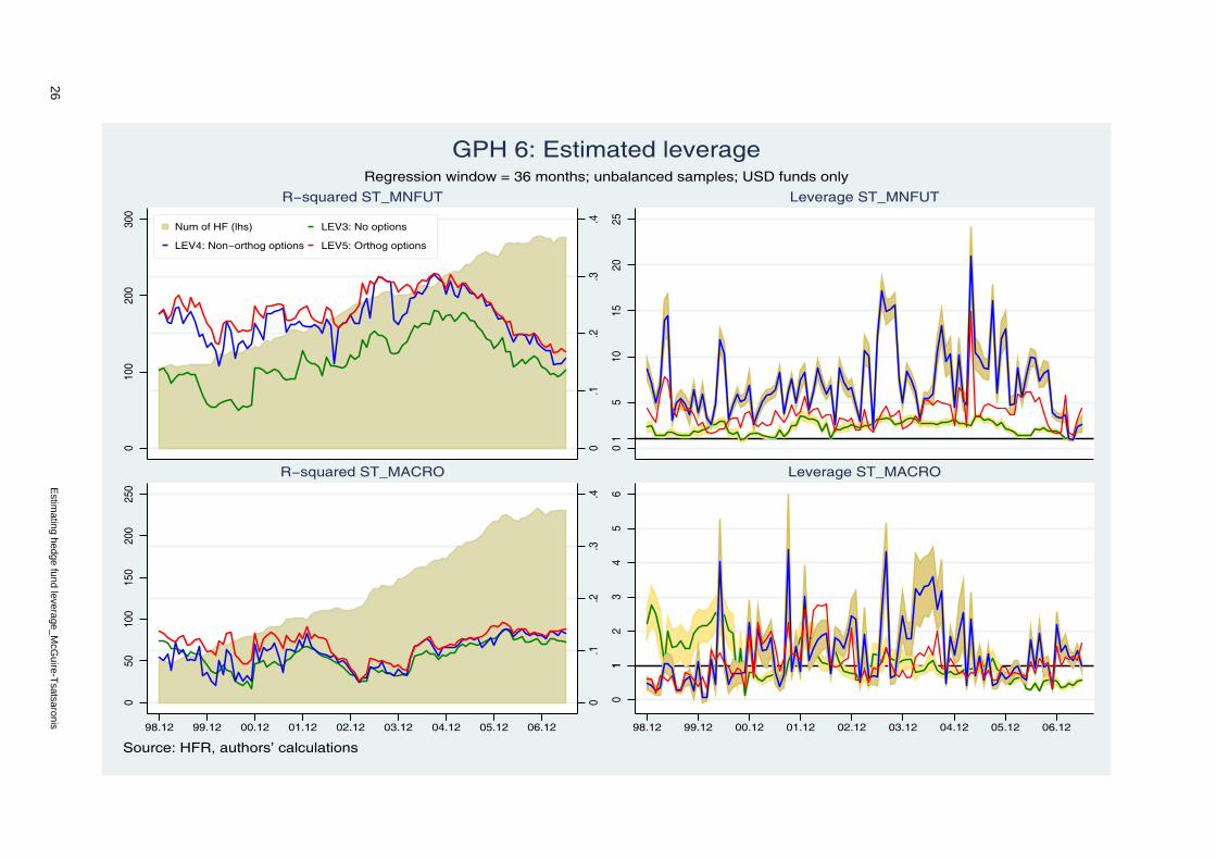
26

0.1

.2.3

.4

010

020

030

0



R−squared ST_MNFUT

05

1015

2025

1

Leverage ST_MNFUT

0.1

.2.3

.4

050

100

150

200

250

98.12 99.12 00.12 01.12 02.12 03.12 04.12 05.12 06.12

R−squared ST_MACRO

01

23

45

61

98.12 99.12 00.12 01.12 02.12 03.12 04.12 05.12 06.12

Leverage ST_MACRO




Estim


uire-Tsatsaronis

Estim


uire-Tsatsaronis

0.1

.2.3

.4

050

100

150

200

250



R−squared ST_RVALARB

0.5

11.

52

2.5

31

Leverage ST_RVALARB

0.1

.2.3

.4

010

020

030

0

98.12 99.12 00.12 01.12 02.12 03.12 04.12 05.12 06.12

R−squared ST_FXINC

0.5

11.

52

1

98.12 99.12 00.12 01.12 02.12 03.12 04.12 05.12 06.12

Leverage ST_FXINC




27

28

.1.1

5.2

.25

0.0

2.0

4.0

6.0

8.1

Ave Returns (lhs)

Ave Volatility (rhs)

Performance ST_FOF

0.2

.4.6

0020

040

060

080

00

Num of HFs (lhs)

LEV3 R2 (rhs)

R−squared and sample size ST_FOF

.4.6

.81

1.2

1.4

1.6

1

LEV3

Leverage ST_FOF

.2.3

.4.5

.6.7

0.0

5.1

.15

.2

98.12 99.12 00.12 01.12 02.12 03.12 04.12 05.12 06.12

Performance ST_EQHED

0.1

.2.3

.400

200

400

600

800

0

98.12 99.12 00.12 01.12 02.12 03.12 04.12 05.12 06.12

R−squared and sample size ST_EQHED

.51

1.5

22.

51

98.12 99.12 00.12 01.12 02.12 03.12 04.12 05.12 06.12

Leverage ST_EQHED


Thick lines: funds which report using leverage; Thin lines: funds which report using no leverage

GPH 8: Estimated and reported leverage

Estim


uire-Tsatsaronis

Estim


uire-Tsatsaronis

.3.4

.5.6

0.0

5.1

.15

Ave Returns (lhs)


Performance ST_MNFUT

0.0

5.1

.15

.2.2

500

5010

015

020

00

Num of HFs (lhs)

LEV3 R2 (rhs)

R−squared and sample size ST_MNFUT

01

23

41

LEV3

Leverage ST_MNFUT

.25

.3.3

5.4

.45

.5

0.0

5.1

.15

98.12 99.12 00.12 01.12 02.12 03.12 04.12 05.12 06.12

Performance ST_MACRO

0.0

5.1

.15

0050

100

150

200

0

98.12 99.12 00.12 01.12 02.12 03.12 04.12 05.12 06.12

R−squared and sample size ST_MACRO

0.5

11.

52

2.5

1

98.12 99.12 00.12 01.12 02.12 03.12 04.12 05.12 06.12

Leverage ST_MACRO




29

30

.3.4

.5.6

.7.8

−.1

0.1

.2

Ave Returns (lhs)


Performance ST_EQNOHED

0.2

.4.6

0020

4060

800

Num of HFs (lhs)

LEV3 R2 (rhs)

R−squared and sample size ST_EQNOHED

.81

1.2

1.4

1.6

1.8

1

LEV3

Leverage ST_EQNOHED

.15

.2.2

5.3

.35

0.0

5.1

.15

98.12 99.12 00.12 01.12 02.12 03.12 04.12 05.12 06.12

Performance ST_EVNTDRV

0.2

.4.6

0050

100

150

200

0

98.12 99.12 00.12 01.12 02.12 03.12 04.12 05.12 06.12

R−squared and sample size ST_EVNTDRV

0.5

11.

52

1

98.12 99.12 00.12 01.12 02.12 03.12 04.12 05.12 06.12

Leverage ST_EVNTDRV




Estim


uire-Tsatsaronis

Estim


uire-Tsatsaronis .11

.12

.13

.14

0.0

2.0

4.0

6.0

8

Ave Returns (lhs) Ave Volatility (rhs)

Performance ST_FOF

0.2

.4.6

.800

5010

015

020

025

00



R−squared and sample size ST_FOF

02

46

81

Leverage ST_FOF

.25

.3.3

5.4

.45

.5

0.0

5.1

.15


Performance ST_EQHED

0.1

.2.3

.400

5010

015

020

00



R−squared and sample size ST_EQHED

01

23

45

1

Leverage ST_EQHED

.35

.4.4

5.5

.55

0.0

5.1

.15

02.12 03.12 04.12 05.12 06.12 07.06


Performance ST_MNFUT

0.1

.2.3

.400

2040

6080

0

02.12 03.12 04.12 05.12 06.12 07.06



R−squared and sample size ST_MNFUT

05

1015

201

02.12 03.12 04.12 05.12 06.12 07.06

Leverage ST_MNFUT


Regression window = 36 months, USD funds only, samples balanced from Jan 2000 to June 2007

GPH A2.1: Estimated leverage, balanced samples

31

32

−.2

−.1

0.1

.2.3

−.2

−.1

0.1

.2.3

LEV3: No options (lhs)

LEV4: Non−orthog options (lhs)

Sensitivity to SMB

−.15

−.1

−.05

0.0

5.1

.15

.2.2

5

−.15

−.1

−.05

0.0

5.1

.15

.2.2

5

Sensitivity to 3M_fjp_tnz

−1−.

50

.51

−1−.

50

.51

Sensitivity to FRB_MC

−.04

−.03

−.02

−.01

0.0

1.0

2.0

3.0

4

−.6

−.4

−.2

0.2

.4.6

98.12 99.12 00.12 01.12 02.12 03.12 04.12 05.12 06.12

LEV4: Synthetic Call (rhs)

LEV4: Synthetic Put (rhs)

Sensitivity to SP500

−.08

−.06

−.04

−.02

0.0

2.0

4.0

6.0

8

−3−2

−10

12

34

98.12 99.12 00.12 01.12 02.12 03.12 04.12 05.12 06.12

Sensitivity to SBWGBIUSD

−.1

−.05

0.0

5.1

−2−1

.5−1

−.5

0.5

11.

52

98.12 99.12 00.12 01.12 02.12 03.12 04.12 05.12 06.12

Sensitivity to GSCOM

Source: Authors’ calculations

Coefficient estimates on various risk factors, estimated using models LEV3 (red) and LEV4 (blue), USD funds only

GPH A3.1: ST_FOF Sensitivity to risk factors

Estim


uire-Tsatsaronis

Estim


uire-Tsatsaronis

0.0

5.1

.15

.2.2

5.3

.35

.4

0.0

5.1

.15

.2.2

5.3

.35

.4



Sensitivity to SMB

−.15

−.1

−.05

0.0

5.1

.15

.2

−.15

−.1

−.05

0.0

5.1

.15

.2


−1−.

8−.

6−.

4−.

20

.2.4

−1−.

8−.

6−.

4−.

20

.2.4


−.04

−.03

−.02

−.01

0.0

1.0

2.0

3.0

4

−.8

−.6

−.4

−.2

0.2

.4.6

.8

98.12 99.12 00.12 01.12 02.12 03.12 04.12 05.12 06.12




−.08

−.06

−.04

−.02

0.0

2.0

4.0

6.0

8

−4−3

−2−1

01

23

4

98.12 99.12 00.12 01.12 02.12 03.12 04.12 05.12 06.12


−.06

−.04

−.02

0.0

2.0

4.0

6

−1.5

−1−.

50

.51

1.5

98.12 99.12 00.12 01.12 02.12 03.12 04.12 05.12 06.12




GPH A3.2: ST_EVNTDRV Sensitivity to risk factors

33

34

0.1

.2.3

.4.5

.6.7

0.1

.2.3

.4.5

.6.7



Sensitivity to SMB

−.2

−.1

0.1

.2.3

.4

−.2

−.1

0.1

.2.3

.4


−1−.

50

.51

1.5

−1−.

50

.51

1.5


−.04

−.03

−.02

−.01

0.0

1.0

2.0

3.0

4

−.8

−.6

−.4

−.2

0.2

.4.6

.8

98.12 99.12 00.12 01.12 02.12 03.12 04.12 05.12 06.12




−.1

−.05

0.0

5.1

−6−4

−20

24

6

98.12 99.12 00.12 01.12 02.12 03.12 04.12 05.12 06.12


−.08

−.06

−.04

−.02

0.0

2.0

4.0

6.0

8

−2−1

.5−1

−.5

0.5

11.

52

98.12 99.12 00.12 01.12 02.12 03.12 04.12 05.12 06.12




GPH A3.3: ST_EQHED Sensitivity to risk factors

Estim


uire-Tsatsaronis

0.1

.2.3

.4.5

0.1

.2.3

.4.5



Sensitivity to SMB

−.2

−.1

0.1

.2.3

.4

−.2

−.1

0.1

.2.3

.4


−.7

−.6

−.5

−.4

−.3

−.2

−.1

0

−.7

−.6

−.5

−.4

−.3

−.2

−.1

0


−.05

0.0

5

−1−.

50

.51

98.12 99.12 00.12 01.12 02.12 03.12 04.12 05.12 06.12




−.05

0.0

5

−3−2

−10

12

34

98.12 99.12 00.12 01.12 02.12 03.12 04.12 05.12 06.12


−.03

−.02

−.01

0.0

1.0

2.0

3

−.6

−.4

−.2

0.2

.4.6

.8

98.12 99.12 00.12 01.12 02.12 03.12 04.12 05.12 06.12




GPH A3.4: ST_EQNOHED Sensitivity to risk factors

Estim


uire-Tsatsaronis 35

BIS Working Papers · funds of funds, macro funds, equity funds, etc) yields time-varying estimates...

Documents

Transcript of BIS Working Papers · funds of funds, macro funds, equity funds, etc) yields time-varying estimates...