Biostatistics

Lecture 12 5/11 & 5/12/2015

Ch 10 – Hypothesis Testing

Introduction

• CI (confidence interval) provides a way of estimating whether our sample is good enough to provide a realistic statistics to the real population.

• In many of our examples mentioned earlier, we tried to find whether the mean the mean value of a sample (of limited size)value of a sample (of limited size) is realistic to represent the true mean the true mean value of the population (much larger value of the population (much larger size)size).

Cont’d

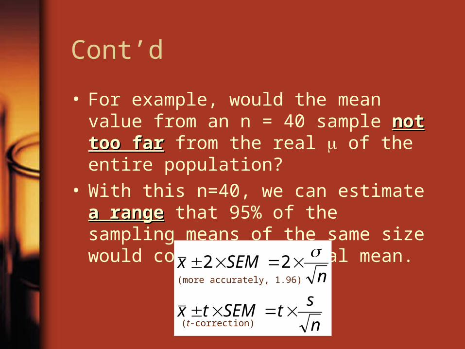
• For example, would the mean value from an n = 40 sample not too farnot too far from the real of the entire population?

• With this n=40, we can estimate a rangea range that 95% of the sampling means of the same size would contain the actual mean.

n

stSEMtx

nSEMx

22(more accurately, 1.96)

(t-correction)

Hypothesis Testing

• The other wayThe other way of making sure whether your collected sample (of limited sample size) is good enough (to represent the true statistics of the population) is to do a hypothesis testinghypothesis testing ((假說檢定假說檢定 )).

• How would we conclude that a How would we conclude that a computed mean value computed mean value (previously we (previously we called it called it x̅� x̅� ) would be ) would be acceptableacceptable to act to act as the actual mean of the population as the actual mean of the population (previously we called it (previously we called it )?)?

Cont’d

• To perform such a test, we begin by claiming that the population mean equalsequals to some postulated (假定的 ) value 0.

• We will have two hypotheses:

– one called a null hypothesisnull hypothesis, or H0,

– the other called alternative alternative hypothesishypothesis, or HA.

Cont’d

• For example, HH00 : : = = 00 = 211 = 211 is a null hypothesis that we thinkthink the computed sample mean would be the same as the actual mean.

• The second statement that contradictscontradicts

((矛盾矛盾 )) H0 , would be HHAA : : 211 211.

• One of the two statements One of the two statements must be true.must be true.

Cont’d

• We would rejectreject the null hypothesis, if

there is not enough evidencenot enough evidence to show that the computed sample mean would be the same as the actual mean.

• So it is a matter of So it is a matter of ““to rejectto reject”” or or

““not to rejectnot to reject”” the null the null hypothesis.hypothesis.

Implementation

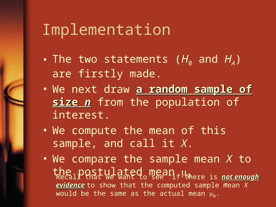
• The two statements (H0 and HA) are firstly made.

• We next draw a random sample of size a random sample of size nn from the population of interest.

• We compute the mean of this sample, and call it X.

• We compare the sample mean X to the postulated mean 0

Recall that we want to see “if there is not enough evidencenot enough evidence to show that the computed sample mean X would be the same as the actual mean 0.”

Cont’d

• Specifically, we want to know whether the whether the differencedifference between these two means ( between these two means (XX and and 00) is too large to be attributed to ) is too large to be attributed to

chance alone (chance alone (純屬巧合純屬巧合 )). [If so, then . [If so, then many other sample means would not be many other sample means would not be that far off the actual mean.]that far off the actual mean.]

• The other way of saying this is to see if The other way of saying this is to see if their difference is their difference is not likely to be bignot likely to be big.

• In these cases, we DO NOT REJECT the null hypothesis. That is, we think the presented sample mean is good.

A brief summary

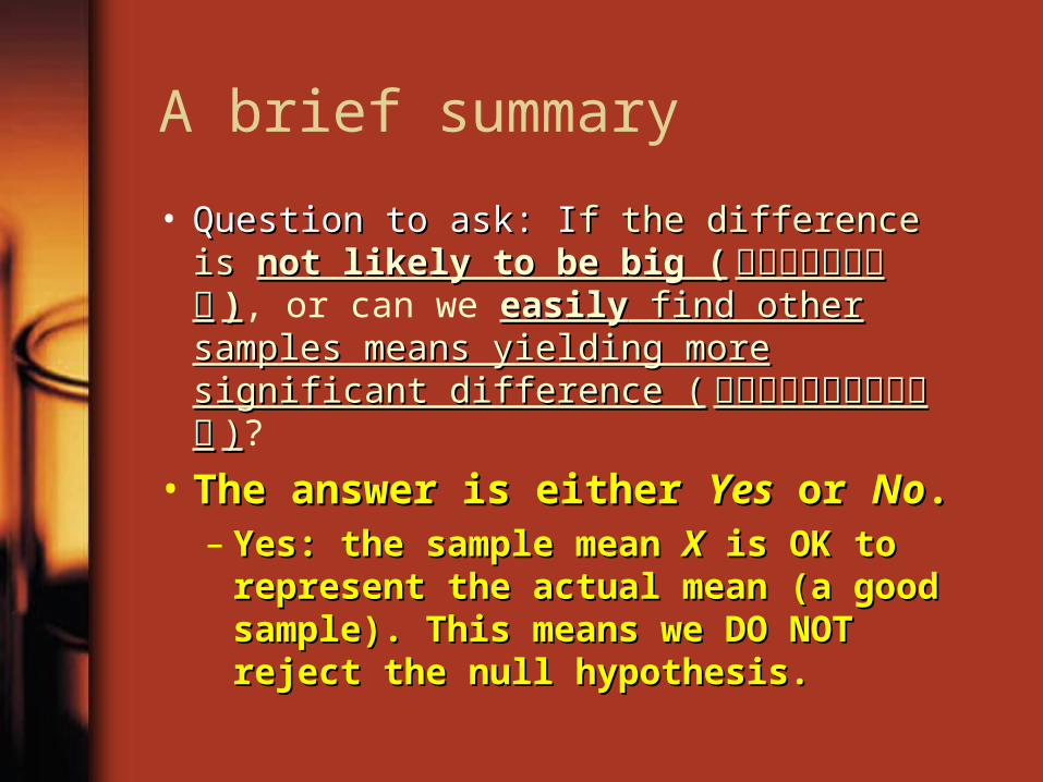
• Question to ask: IQuestion to ask: If the difference is f the difference is not not likely to be big (likely to be big ( 差異大的機率很低差異大的機率很低 )), or can we easilyeasily find other samples means find other samples means yielding more significant difference (yielding more significant difference ( 容易容易找到差異更大的例子找到差異更大的例子 ))?

• The answer is either The answer is either YesYes or or NoNo..– Yes: the sample mean Yes: the sample mean XX is OK to is OK to

represent the actual mean (a good represent the actual mean (a good sample). This means we DOsample). This means we DO NOT NOT reject the null hypothesis.reject the null hypothesis.

(1) (1) RejectingRejecting the Hypothesis

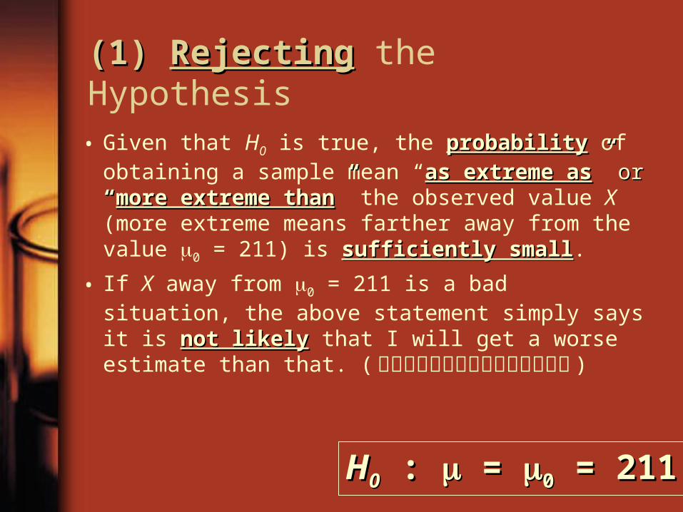
• Given that H0 is true, the probabilityprobability of obtaining a sample mean “as extreme asas extreme as”” or or ““more extreme thanmore extreme than”” the observed value X (more extreme means farther away from the value 0 = 211) is sufficiently smallsufficiently small.

• If X away from 0 = 211 is a bad situation, the above statement simply says it is not likelynot likely that I will get a worse estimate than that. (不太可能再得到這麼極端的平均值 )

HH00 : : = = 00 = 211 = 211

Cont’d

• In this case, the data are not compatiblenot compatible with the null hypothesis, where we think our sample mean would be equal to the actual mean. So we rejectreject the hypothesis.

• The result would now be more supportivesupportive to HA. That is, our sampling is not likely to get a mean that is close to the actual mean value.

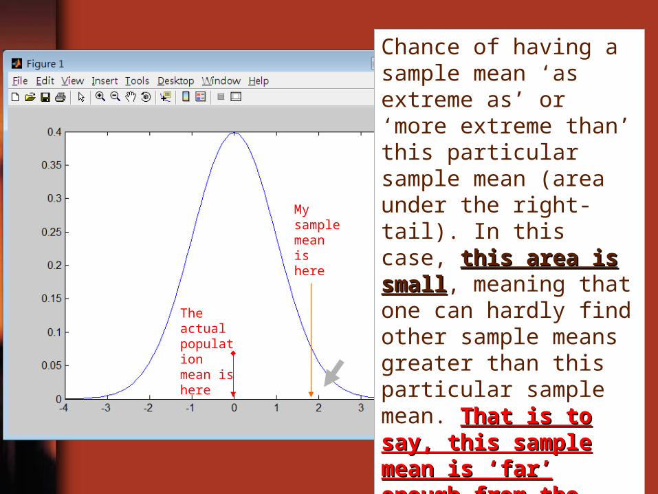
The actual population mean is here

My sample mean is here

Chance of having a sample mean ‘as extreme as’ or ‘more extreme than’ this particular sample mean (area under the right-tail). In this case, this area is smallthis area is small, meaning that one can hardly find other sample means greater than this particular sample mean. That is to say, this That is to say, this sample mean is ‘far’ sample mean is ‘far’ enough from the actual enough from the actual mean, and we would fail mean, and we would fail to satisfy the null to satisfy the null hypothesis.hypothesis.

(2) (2) Not RejectingNot Rejecting the Hypothesis

• If there is not enough evidence to doubtnot enough evidence to doubt the validity of the null hypothesis (a ‘not-so-small’ tail in previous slide, for example), we cannotcannot reject this claim.

• However, we do not say we accept HHowever, we do not say we accept H00. The . The test does not “prove” the null hypothesis. test does not “prove” the null hypothesis.

• It is still very likely that the actual mean value would not be 211. For example, when the sample size is too small, we may not be able to easily prove the sample mean is far from the actual mean.

Analogy with the Justice System (司法系統 )

Court of Law1. Start with premise that person

is innocent. (Opposite is guilty.)

2. If enough evidence is found to show beyond reasonable doubt that person committed crime, reject premise. (Enough evidence that person is guilty.)

3. If not enough evidence found, we don’t reject the premise. (Not enough evidence to conclude a person guilty.)

Statistical Hypothesis Test1. Start with null hypothesis.

(Opposite is alternative hypothesis.)

2. If a significant amount of evidence is found to refute( 駁斥 ) null hypothesis, reject it. (Enough evidence to conclude alternative is true.)

3. If not enough evidence found, we don’t reject the null. (Not enough evidence to disprove null.)

How “Small” is Sufficiently “Small”?• In most cases, 0.050.05 is considered a small

probability.• Thus we reject the null hypothesis when

the chance that the sample could have come from a population with mean = 0 = 211 is less than or equal to 5%. (The sample is not significantnot significant, or too too insignificantinsignificant to represent the whole population.)

Cont’d

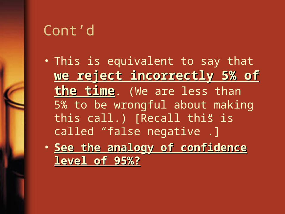
• This is equivalent to say that we reject we reject incorrectly 5% of the timeincorrectly 5% of the time. (We are less than 5% to be wrongful about making this call.) [Recall this is called “false negative”.]

• See the analogy of confidence level of See the analogy of confidence level of 95%?95%?

Significant Level of the Test

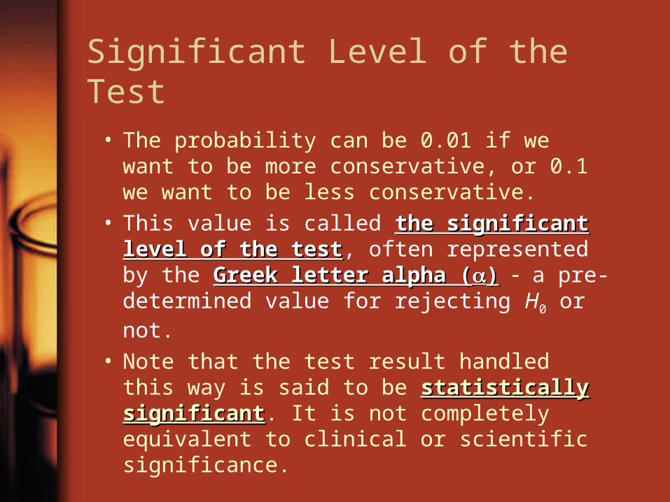
• The probability can be 0.01 if we want to be more conservative, or 0.1 we want to be less conservative.

• This value is called the significant level the significant level of the testof the test, often represented by the Greek letter alpha (Greek letter alpha ()) a pre-determined value for rejecting H0 or not.

• Note that the test result handled this way is said to be statistically significantstatistically significant. It is not completely equivalent to clinical or scientific significance.

P-value

• The probability of obtaining a mean as as extreme or more extremeextreme or more extreme than the observed sample mean X, given that the null hypothesis is truenull hypothesis is true, is called the p-value. (the area under the tail(s))

• If p is equal to or smaller than the pre-determined significance level , we rejectreject the hypothesis.

• If not, we do not rejectdo not reject the hypothesis. (Recall that we don’t reject it does not mean we accept it.)

Example 1

• An experiment is performed to determine whether a coin flip is fair (50% chance of landing on heads or tails) or unfairly biased, either toward heads (> 50% chance of landing heads) or toward tails (< 50% chance of landing heads). (A bent coin produces biased results.)

• Since we consider both biased alternatives, a two-tailed testtwo-tailed test is performed.

• The null hypothesis is that the coin is The null hypothesis is that the coin is fairfair.

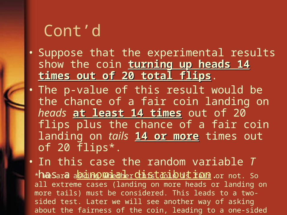
Cont’d• Suppose that the experimental results show the

coin turning up heads 14 times out of 20 total turning up heads 14 times out of 20 total flipsflips.

• The p-value of this result would be the chance of a fair coin landing on heads at least 14 timesat least 14 times out of 20 flips plus the chance of a fair coin landing on tails 14 or more14 or more times out of 20 flips*.

• In this case the random variable T has a binomial distribution.

* We are asking whether this coin is fair or not. So all extreme cases (landing on more heads or landing on more tails) must be considered. This leads to a two-sided test. Later we will see another way of asking about the fairness of the coin, leading to a one-sided test.

Cont’d

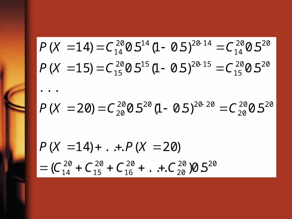
• Recall that in binomial distribution (in chapter 7) we have the formula

• In this case, In this case, n n = 20, and = 20, and p p = 0.5. So for = 0.5. So for the probability of showing 14 or more the probability of showing 14 or more heads for 20 clips, we’d like to heads for 20 clips, we’d like to compute compute PP((XX=14)+ =14)+ PP((XX=15)+ =15)+ PP((XX=16)+=16)+… … PP((XX=20).=20).

xnxnx ppCxXP )1()(

202020

2016

2015

2014

202020

2020202020

202015

1520152015

202014

1420142014

5.0)...(

)20(...)14(

5.0)5.01(5.0)20(

...

5.0)5.01(5.0)15(

5.0)5.01(5.0)14(

CCCC

XPXP

CCXP

CCXP

CCXP

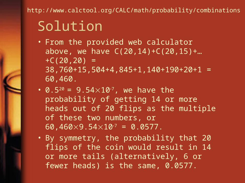
Solution• From the provided web calculator above, we

have C(20,14)+C(20,15)+…+C(20,20) = 38,760+15,504+4,845+1,140+190+20+1 = 60,460.

• 0.520 = 9.54107, we have the probability of getting 14 or more heads out of 20 flips as the multiple of these two numbers, or 60,4609.54107 = 0.0577.

• By symmetry, the probability that 20 flips of the coin would result in 14 or more tails (alternatively, 6 or fewer heads) is the same, 0.0577.

http://www.calctool.org/CALC/math/probability/combinations

MATLAB’s binopdf

>>binopdf(1414,20,0.5)+binopdf(1515,20,0.5)+binopdf(1616,20,0.5)+binopdf(1717,20,0.5)+binopdf(1818,20,0.5)+binopdf(1919,20,0.5)+binopdf(2020,20,0.5)

ans = 0.0577

>>

BINOPDF Binomial probability density function.

Y = BINOPDF(X,N,P) returns the binomial probability density function with parameters N and P at the values in X. Note that the density function is zero unless X is an integer.

MATLAB’s binocdf

>>1-binocdf(13,20,0.5)ans = 0.0577>>

Similar to other cumulative density functions (CDFs), one can easily use BINOCDF to compute for the answer from previous slide:

Cont’d

• Thus, the p-value for the coin turning up the same face (either head or tail)14 times out of 20 total flips is 0.0577 + 0.0577 = 0.11540.1154.

• The calculated p-value exceeds 0.05The calculated p-value exceeds 0.05, so the observation is consistent with the null hypothesis — that the observed result of 14 heads out of 20 flips can be ascribed to chance alonechance alone — as it falls within the range of what would happen 95% of the time.

Cont’d

• In our example, we fail to rejectfail to reject the null hypothesis at the 5% level.

• Although the coin did not fall evenly, the deviation from expected outcome is just small enough to be reported as being "not statistically significant at the 5% level".

• Of course, like we said earlier, "not statistically significant at the 5% level“ does not necessarily mean it is a fair coin.

Cont’d

• However, had a single extra head been obtained, the resulting p-value (two-tailed) would be 0.0414 (4.14%). [Try this for [Try this for yourself…]yourself…]

• This time the null hypothesis - that the observed result of 15 heads out of 20 flips can be ascribed to chance alone - is rejectedrejected.

• Such a finding would be described as being "statistically significant at the 5% level".

Comments

• Although we said that doing hypothesis testing at the significant level of 0.05 is equivalent of estimating a 95% CI, it is apparent in this case that one cannot really compute the CI in this coin-flipping scenario. (We do not have needed parameters such as mean value, standard deviations, etc. as we did in previous chapter.)

10.2 Two-sided Tests

• We have already seen, from the previous coin-flipping example, to determine whether a coin is fair or not.

• In that case, a two-tailed test is performed, meaning that we consider the we consider the sum of the two tailed-areas under the sum of the two tailed-areas under the binomial distribution as the p-valuebinomial distribution as the p-value.

• This is exactly what a two-sided test means.

Z-test

• Assume that a continuous random variable X has mean 0 and known known

standard deviation standard deviation .• According the central limit theorem, the

following normalization would give the variable Z a standard normal distribution if n is large enough.

n

XZ

/0

Cont’d

• We may now consider a value of Z that is as extremeas extreme or more extreme thanmore extreme than the one observed, say, a mean value X, to set up a null hypothesis and to test on it just like we did in the coin flipping example.

• Because it relies on the standard Because it relies on the standard normal distribution, a test of this kind is normal distribution, a test of this kind is called a called a zz-test.-test.

t-test

• When the real standard deviation (for the general population) is not known, we would substitute the sample value sample value standard deviation standard deviation ss for . This alternatively gives the following formula.

• If the underlying population is normally distributed, the random variable t has a t distribution with n1 degree of freedom.

ns

Xt

/0

Cont’d

• Based on this value of t on the t distribution (similar to the value of z on the standard normal distribution, and recall that a t distribution is a “stepped-on” standard normal distribution), again, we may test whether the probability of obtaining a sample mean that is more extreme than the one observed.

• This procedure is known as a t-test.

Example 2

• Given distribution of serum cholesterol levels for adult males in US who are hypertensive and smokinghypertensive and smoking, with = 46.

• The null hypothesis to be tested is

H0: = 211,

where 0 = 211 is the mean for allall 20- to 74-yr-old males.

Note that the subjects under investigation (hypertensive & smoking) are apparent different than all 20- to 74-yr-old males.

Why would we like to establish this null hypothesis? What are we ex̅pecting to see?

Example 2 – cont’d

• We now have a group of 12 hypertensive smokers of mean x=217.

• Is it likely that this sample mean Is it likely that this sample mean (hypertensive) would be any (hypertensive) would be any different than the mean of 211 from different than the mean of 211 from all adult males?all adult males? – What will be concluded if the answer is

Yes? What will be if the answer is No?

• Should this be a z-test or t-test? One-sided or two-sided?

Solution

• This should be a z-test, since the population STD is known as 46.

• This should be a two-sided test, since much greater than 211 or much smaller than 211 are both being considered as “different than 211”.

Solution

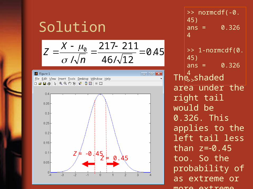
45.012/46

211217

/0

n

XZ

Z = 0.45

The shaded area under the right tail would be 0.326. This applies to the left tail less than z=0.45 too. So the probability of as extreme or more extreme, or the p-value, is 0.6520.652.

Z = 0.45

>> normcdf(-0.45)ans = 0.3264

>> 1-normcdf(0.45)ans = 0.3264>>

Cont’d

• So the p-value is 0.625, which is far bigger than the ordinary 0.05 threshold.

• Therefore we do not rejectdo not reject the null hypothesis.

• The evidence is not sufficient to conclude that the serum cholesterol level of the population of hypertensive smokers is different from 211, which is the mean value from the whole 20- to -74-yr-old US males. [Cannot say the difference is significant!]

Cont’d

• In other words, we CANNOT say, from this 12-person sampling and statistics, that being hypertensive and smoking would cause the raise of serum cholesterol level.

Analogy to CI

• In fact, we already learned that the area beyond two tails is 5% when z=±1.96.

• That is, this often used 0.05 statistically significant level is mathematically equivalent to the 95% confidence interval from z=1.96 to z=1.96.

• In other words, hypothesis testing and hypothesis testing and CI estimation are basically the same CI estimation are basically the same concept in judging how good the concept in judging how good the sample statistics are comparing with sample statistics are comparing with the population statistics.the population statistics.

Cont’d

• Following the previous example, 95% the conference interval is found to be 217±1.96*46/sqrt(12)=217±26=(191, 243).

• The mean serum cholesterol level from all US males is 211, which is within 95% CI.

• Therefore, we do not reject the null hypothesis that these two mean values are “close”.

• Mean cholesterol levels from both groups are comparable.

Summary

• Although CI and tests of hypotheses both lead us to the same conclusion, the information they provided is somewhat different.

• CI supplies a range of reasonable values for the mean value , and tells us something about the uncertainty in our point estimate x[ .

• The hypothesis test helps to decide whether the postulated mean value 217 is likely to be correct or not (to 211), with a specific p-value.

Example 3

• Given two populations – all infants receiving antacids that contain aluminum, and all infants not receiving antacids.

• Their plasma aluminum levels were recorded.

• All infants receiving antacids have no known and . For those infants receiving no antacids, = 4.13.

Cont’d• 10 children were selected from all infants

receiving antacids, with plasma aluminum level x̅! =37.20 and s=7.13.

• Note that the two means are very different (37.20 vs 4.13). However, STD=7.13, which may not be small enough to justify the two means are very different.

• Is it likely that the data in our sample could have come from a population with =4.13? That is, we want to test the null hypothesis

HH00 : : = = 00 = 4.13 = 4.13

Cont’d

• 2-sided test with =0.05.• t-test is used rather than z-test.

• t=2.2622 to give 5% of the two tails in a t-distribution with df=10-1=9. Our computed t=14.67 is much going into the tail end.

• A very small p-value is expected.

67.1410/13.7

13.42.37

/0

ns

xt

>> tinv(0.975,9)ans = 2.2622>>

Cont’d

• The computed p-value is smaller than prescribed =0.05.

• We therefore reject the null hypothesis. • That is, the “mean plasma aluminum level

of children receiving antacids” is NOT EQUAL TO the “mean plasma aluminum level of children who do not receive them”.

• Taking antacids will result in different plasma aluminum level for children.

>> 2*(1-tcdf(14.67, 9))ans = 1.3683e-007>>

Comments

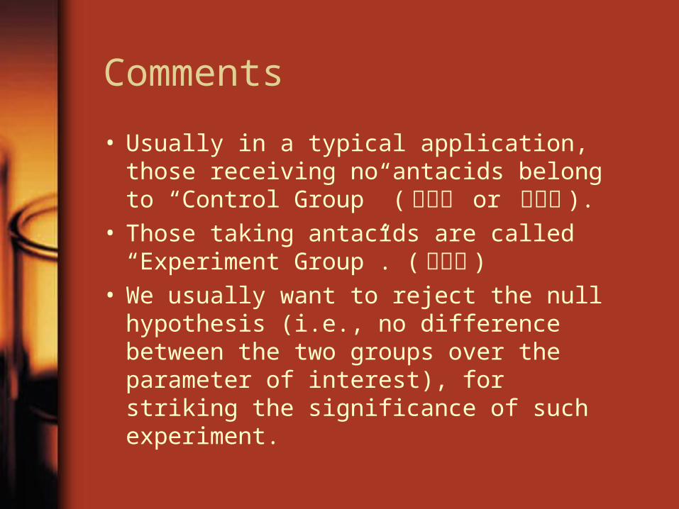
• Usually in a typical application, those receiving no antacids belong to “Control Group” ( 控制組 or 對照組 ).

• Those taking antacids are called “Experiment Group”. ( 實驗組 )

• We usually want to reject the null hypothesis (i.e., no difference between the two groups over the parameter of interest), for striking the significance of such experiment.

10-3 One-sided Tests

• Similar to what’s learned from estimating a confidence interval, here we also have one-sided tests of hypothesis.

• One such example would be to test whether a coin is biased towards headsis biased towards heads – only large numbers of heads would be significant.

Example 4

• Tossing a coin 5 times and all landed on head.

• Is this enough to say the coin is biased to show more heads?

• Statistically, we are asking whether this coin is biased towards heads at a level of =0.05?

• The null hypothesis would be that the coin is not biased towards heads (note that it is allowed to be biased towards tails, though).

Solution• What is the probability of having 5 or more heads?

• This p-value is significant (less than 0.05) in rejecting the null hypothesis.

>> binopdf(5,5,0.5)ans = 0.0313>>

Comments

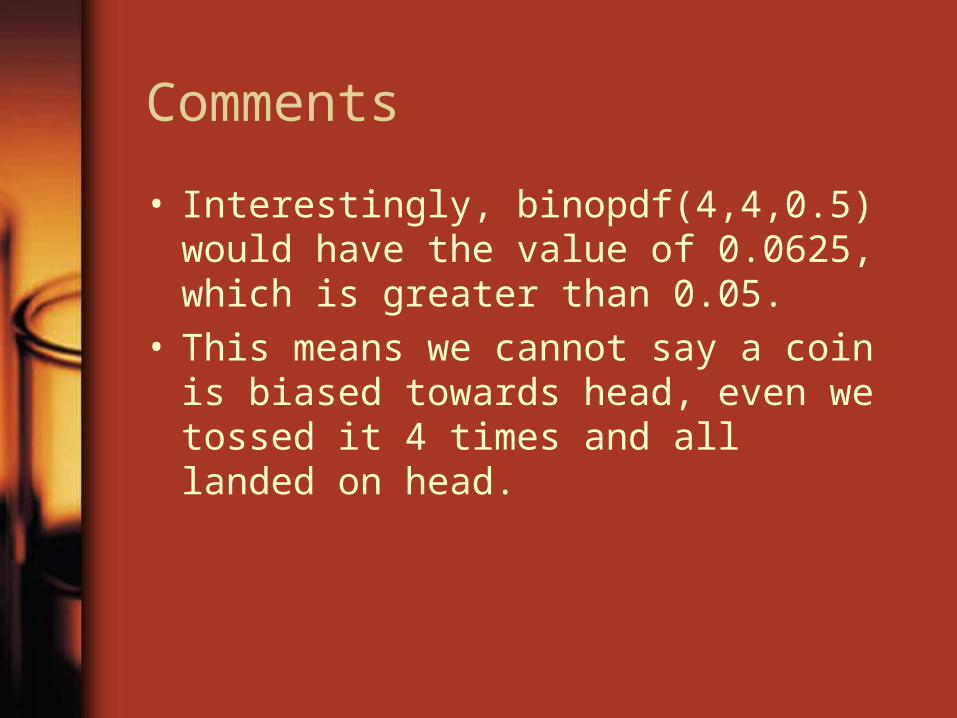
• Interestingly, binopdf(4,4,0.5) would have the value of 0.0625, which is greater than 0.05.

• This means we cannot say a coin is biased towards head, even we tossed it 4 times and all landed on head.

10.4 Types of Error

• Two types of errors occur when a hypothesis test is conducted.

• Type I errorType I error (or rejection error, or error)

• Type II errorType II error (or acceptance error, or error)

= P(reject H0 | H0 is true)

= P(do not reject H0 | H0 is false)

Cont’d

• Apparently, type I error is equivalent to earlier mentioned “False Negative (FN)” (if you consider rejecting the null hypothesis is negative), and type II error is indeed “False Positive (FP)”.

Result of Test

Postulation

= 0 ≠ 0

Do Not Reject

Correct (TP or 1 － )

Type II Error (FP or )

RejectType I Error

(FN or )Correct (TN or 1 － )

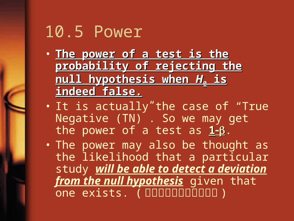
10.5 Power• The power of a test is the probability of The power of a test is the probability of

rejecting the null hypothesis when rejecting the null hypothesis when HH00 is indeed false.is indeed false.

• It is actually the case of “True Negative (TN)”. So we may get the power of a test as 11.

• The power may also be thought as the likelihood that a particular study will be able to detect a deviation from the null hypothesis given that one exists. ( 可正確偵測出差異的能力 )

Example 5• Considering the serum cholesterol level for 20-20- to 74-to 74-

year-oldyear-old US males. This distribution has =46 with =211.

• Assuming that we do not know Assuming that we do not know =211=211. Instead, we have the data from 20- to 24-year-old20- to 24-year-old US males, and their =180.

• Since old men tend to have higher level than young men, we would expect be greater than 180 for 20- to 74-year-old US males.

• That is, we think there exists a difference we think there exists a difference between 180 and the actual mean cholesterol level of 20- to 74-year-old US males.

Cont’d

• We’d like to conduct a one-sidedone-sided test of the null hypothesis

against the alternative hypothesis

• We’d expect H0 to be rejected. (Because old people tend to have higher cholesterol level).

• If we should reject but failed to reject, If we should reject but failed to reject, then we have a type II error (or false then we have a type II error (or false positive). positive).

HH00 : : 180≦ 180≦

HHAA : : ＞＞ 180180

Wrongfully think that old men would have comparable cholesterol level than young men.

Cont’d

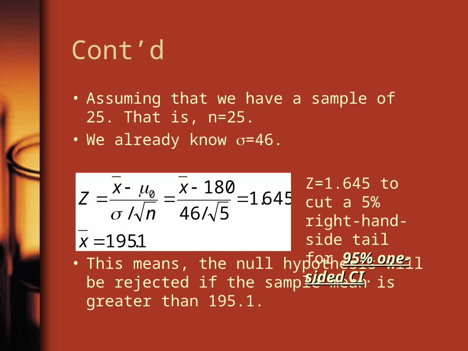
• Assuming that we have a sample of 25. That is, n=25.

• We already know =46.

• This means, the null hypothesis will be rejected if the sample mean is greater than 195.1.

1.195

645.15/46

180

/0

x

x

n

xZ

Z=1.645 to cut a

5% right-hand-side tail for 95% 95% one-sided CIone-sided CI.

>> x=[140:250];>> y1=normpdf(x,180,46/546/5);>> plot(x,y1)

x=195.1

The area under the tail is 0.05.

20- to 24-year-old US males

>> norminv(0.95)ans = 1.6449>> 180+ans*46/5ans = 195.1327>>

Note to use 46/sqrt(25) rather than simply 46. This is the sampling distribution of the means for n=25.

A brief summary

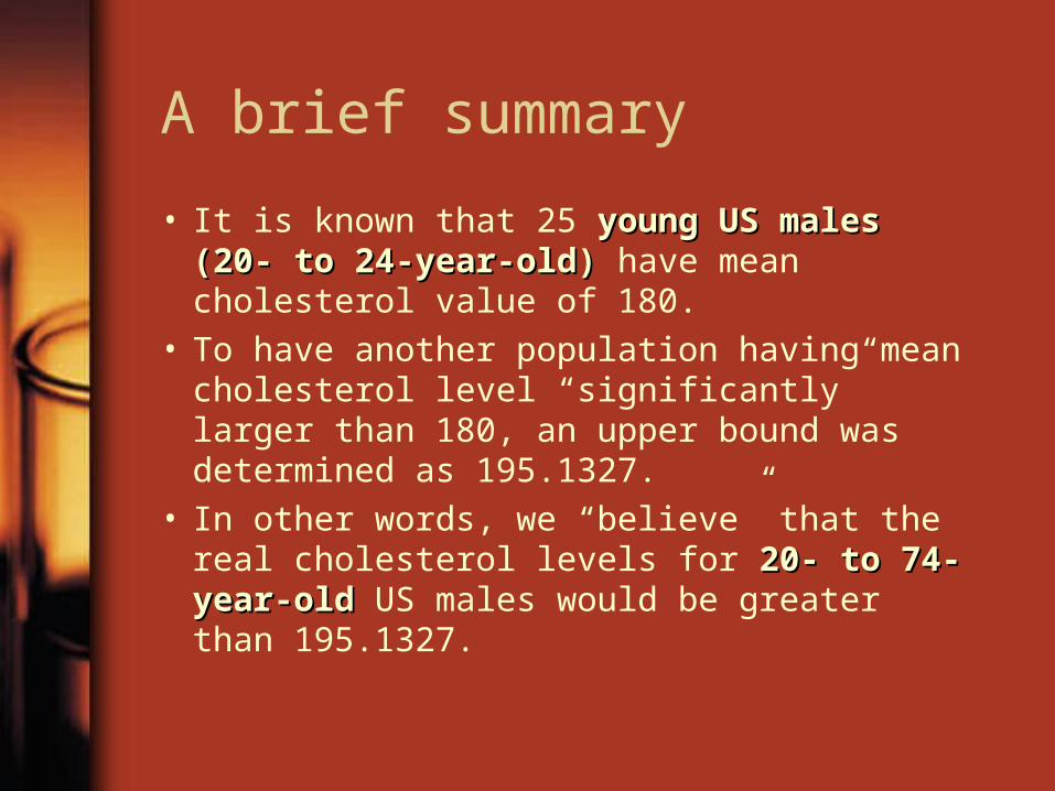
• It is known that 25 young US males (20- young US males (20- to 24-year-old)to 24-year-old) have mean cholesterol value of 180.

• To have another population having mean cholesterol level “significantly” larger than 180, an upper bound was determined as 195.1327.

• In other words, we “believe” that the real cholesterol levels for 20-20- to 74-year-oldto 74-year-old US males would be greater than 195.1327.

• Consider the distribution centered at =211, the realreal one representing serum cholesterol level of 20- to 74-year-old US males.

• This should be the correct distribution, which is shifted to the right of the previous distribution for 20- to 24-year-old US males.

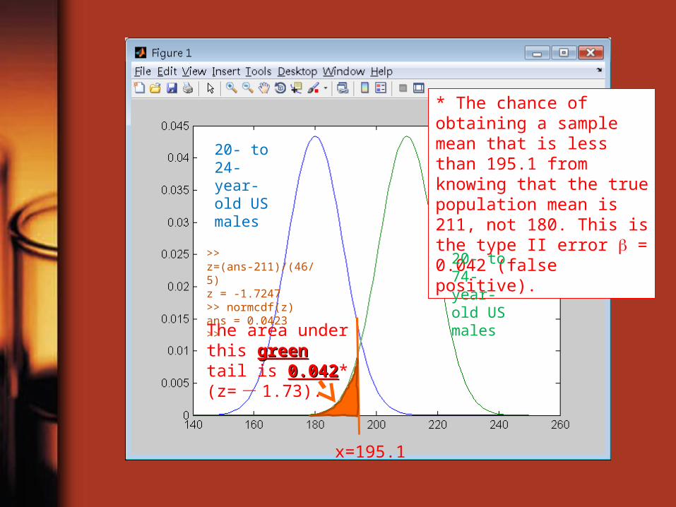
x=195.1

The area under this greengreen tail is 0.0420.042* (z= － 1.73).

* The chance of obtaining a sample mean that is less than 195.1 from knowing that the true population mean is 211, not 180. This is the type II error = 0.042 (false positive).

20- to 24-year-old US males

20- to 74-year-old US males

>> z=(ans-211)/(46/5)z = -1.7247>> normcdf(z)ans = 0.0423>>

Cont’d

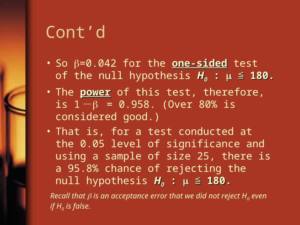
• So =0.042 for the one-sidedone-sided test of the null hypothesis HH00 : : 180.≦ 180.≦

• The powerpower of this test, therefore, is 1 － = 0.958. (Over 80% is considered good.)

• That is, for a test conducted at the 0.05 level of significance and using a sample of size 25, there is a 95.8% chance of rejecting the null hypothesis HH00 : : 180. ≦ 180. ≦

Recall that is an acceptance error that we did not reject H0 even if H0 is false.

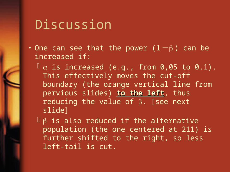
Discussion

• One can see that the power (1 － ) can be increased if: is increased (e.g., from 0,05 to 0.1). This

effectively moves the cut-off boundary (the orange vertical line from pervious slides) to to the leftthe left, thus reducing the value of . [see next slide]

is also reduced if the alternative population (the one centered at 211) is further shifted to the right, so less left-tail is cut.

>> norminv(0.90)ans = 1.2816>> 180+ans*46/5ans = 191.7903191.7903

The area under this greengreen tail is 0.01840.0184* (z= － 2.088).

* The chance of obtaining a sample mean that is less than 191.8 from knowing that the true population mean is 211, not 180. This is the type II error = 0.0184 (false positive).

20- to 24-year-old US males

20- to 74-year-old US males

>> z=(ans-211)/(46/5)z = -2.0880>> normcdf(z)ans = 0.0184>>

Conclusion

• This trade-off between and is similar to that observed between sensitivity and specificity. (Increasing sensitivity may deteriorate specificity)

• The balance between and , however, is a delicate one.

IT IS BETTER THAT 100 IT IS BETTER THAT 100 GUILTY PERSONS SHOULD GUILTY PERSONS SHOULD ESCAPE THAN THAT ONE ESCAPE THAN THAT ONE INNOCENT PERSON INNOCENT PERSON SHOULD SUFFERSHOULD SUFFER

Benjamin FranklinBenjamin Franklin

2nd Midterm Exam

• May 18 (Monday) 2:10~4 pm

• Covering Chapters 7 to 10:– Theoretical probability distributions– Sampling distribution of the mean– Confidence interval– Hypothesis testing