Biostatistics 201A, Midterm Practice Problems With...

Biostatistics 201A, Midterm Practice Problems With Solutions

Inference, Including Estimzation, CIs, Tests and Power

(1) Charity Donations: A charity suspects one of its volunteers of stealing donations. Thevolunteer is going door to door asking for contributions. Past experience shows that honest volun-teers collect on average $3 per household. However, obviously, the actual amount varies for eachhousehold. In the last week the volunteer visited 500 households and the end of the week reportedhis total donations as $1149 with a standard deviation of the amount collected from each personof s = 5.

(a) What is your best estimate of the volunteers average donation per household during this period?

Solution: The best average of the mean is the sample mean. Here we have a total of $1149 indonations from n = 500 houses so we have X = 1149/500 = $2.298 per household. This is certainlya fair percentage lower than previous volunteers. The question is whether it is so much lower as tobe statistically significant (not likely to have happened by chance.)

(b) Find a 95% confidence interval for this volunteer’s average donation based on the data fromthe past week. Based on this interval does the volunteer appear to be typical? Discuss.

Solution: A confidence interval for a single mean is given by

X ± tα/2,n−1s√n

Here we have n = 500 and s = 5. A t-distribution with 500 degrees of freedom is essentially a Zdistribution so we have t.−25,4991.96 and the resulting confidence interval is

2.298± (1.96)5√500

= [1.860, 2.736]

This interval tells us that if we follow this volunteer around for a long time their mean donation perhousehold should be somewhere between $1.86 and $2.74. Since the interval lies entirely below thevalue of $3.00 per household that is typical for this organization the volunteer does NOT appearto be typical. He is taking in less money epr household.

(c) Conduct the hypothesis test an investigator would use to prove the volunteer is stealing. Becareful to state the null and alternative hypotheses, both mathematically and in English, with ajustification and explain your final conclusion. Use α = .025. and compare your result to that ofpart (b).

Solution: Since we specifically want to show the volunteer is stealing we would want to prove thatthey are giving us LESS money than they should. (There is a presumption here that the volunteercollects a normal amount of money, keeps some for himself, and gives us the rest hoping we won’t

1

notice.) Since what we want to prove is the alternative hypothesis we have

H0 : µ ≥ 3–our volunteer turns in as much per household or more than a typical volunteer for thischarity.HA : µ < 3–this volunteer is turning in less money epr household than a typical volunteer.

Our test statistic is

tobs =2.298− 35/√

500= −3.14

Since this is a 1-sided test, our p-value is

P (t499 < −3.14) = P (t.499 > 3.14) = .000895

I got the exact p-value from STATA. During an exam you could approximate it using a t (or forthat matter Z) table as approximately .001. In any case it is smaller than α = .025 so we reject thenull hypothesis and conclude the volunteer is turning in less money than is typical of our volunteers.

(d) Why did I say to use α = .025 in part (c) when you computed a 95% CI in part (b)?

Solution: A confidence interval is a 2-sided quantity. If you have a 95% confidence interval thereis a 2.5% that it misses the true mean by being too high and a 2.5% chance it misses the true meanby being too low. Thus if we want to do a 1-sided test where we care only about low values andwant it to have a comparable value to a 95% CI we need to use α = .− 25 = 2.5%.

(e) Do the results of parts (b) and (c) prove the volunteer is stealing? Give two possible alternativeexplanations.

Solution: The results of (c) and (d) suggest the volunteer is giving us less money than our typ-ical volunteers. However this is NOT the same as proof of stealing!! One possibility is that thisis simply an unlucky sample and the volunteers’s meant ake per household is really higher thanthis. (This doesn’t seem too likely since our p-value was so small but remember that the p-valueisn’t the probability the null is true, it is just the probability of our data ASSUMING the null istrue which is a slightly different thing.) Another possibility is that this volunteer is just incompe-tent and can’t convince people to make donations. Not all volunteers are created equal and average!

(f) What is the effect size for the difference between the volunteer being studied and the agenciestypical volunteers? How big would you consider this effect to be?

Solution: The effect size for a one-sample t-test is simply the difference between the estimatedmean and the hypothesized mean divided by the standard deviation:

d =X − µH0

s=

2.298− 35

= −.14

This is a very small effect size by the standards we learned in class. (Note that as a percentageof the average the effect is pretty big but the standard deviation is very large compared to the

2

mean.) The only reason we have been able to detect this effect so convincingly is that the samplesize (number of houses) is extremely large.

(g) What is the minimum detectable effect size for this study for a two-sided test with α = .05 and80% power? (Note–you need to use STATA to do this as stated. On an exam I would have to giveyou a printout to interpret.) In general do you consider the power here to be high? Discuss.

Solution: I did the calculation on STATA (see results below). The minimum detectable effectsize is d = .13 SDs I also got the minimum detectable effect size for a 1-sided test which is d =.11, slightly smaller. Since the n is so large we could actually do all calculations using Z and couldcompute the power analytically (though I would consider that a hard bonus problem for this class.)The smallest effect size we can detect is very small indeed meaning that our power is excellent.The smaller the effect you can see the stronger the information you have is.

Two-sided test:

. sampsi 0 .13, sd(1) n(500) onesample

Estimated power for one-sample comparison of meanto hypothesized value

Test Ho: m = 0, where m is the mean in the population

Assumptions:

alpha = 0.0500 (two-sided)alternative m = .13

sd = 1sample size n = 500

Estimated power:

power = 0.8282

One-sided test:. sampsi 0 .11, sd(1) n(500) onesample onesided

Estimated power for one-sample comparison of meanto hypothesized value

Test Ho: m = 0, where m is the mean in the population

Assumptions:

3

alpha = 0.0500 (one-sided)alternative m = .11

sd = 1sample size n = 500

Estimated power:

power = 0.7924

(h) Suppose instead of comparing the volunteer from the previous parts of this problem to pre-vious population values we instead had two volunteers, one of whom was the the one above andthe second a volunteer who had averaged X = $3 per donation with s = 4 for 25 donations. (i)Find a confidence interval for the difference in means between the two volunteers. (ii) Perform anappropriate hypothesis test to see if the amounts they collect are different (iii) Give an estimate ofthe effect size for the difference in their average collections.

Solution: The first thing we need to do is find the pooled estimate of the standard deviation. Thisis given by

spooled =

√(n1 − 1)s2

1 + (n2 − 1)s22

n1 + n2 − 2=

√499(52) + 24(42)

523= 4.959

Since the bigger part of the sample had a standard deviation of 5 this is not too surprising. Theconfidence interval is

X2 − X1 ± tα/2,n1+n2−2spooled

√1/n11 + 1/n2

or

3− 2.298± (1.96)(4.959)√

1/500 + 1/25 = [−1.29, 2.69]

This says that the true difference in mean donation per household between the two volunteerscould be anywhere from the first colunteer making $1.29 per house more to the second volunteermaking $2.69 per house more. The interval includes 0 or equivalently has values that correspond toeither of the volunteers making more money so we can’t be sure there is a difference between them.This is a result of the relatively large standard deviation and small sample size for the second vo-luteer. Note that when we were treating this number as a population value it had no variance at all!

The equivalent test has

H0 : µ1 = µ2–there is no difference in average donation between the two volunteers.HA : µ1 6= µ2–there is a difference in average donation between the two volunteers.

The test statistic

4

tobs =X2 − X1

spooled

√1/n1 + 1/n2

=.7021.016

= .69

Under the null hypothesis this has a t-distribution with 523 degrees of freedom (essentially a Zdistribution) and the corresponding p-value is

2P (t523 ≥ .69) = .490

Again I got the exact p-value off of STATA. However even just with a t-table it would be veryobvious that the p-value is large and we fail to reject the null hypothesis. We do not have enoughevidence to say there is a difference in average donation per household between the volunteers.

Finally, we are asked for the effect size corresponding to this comparison which is just the differencein means divided by the pooled estimate of the standard deviation. We have

d =X2 − X1

spooled=

.7024.959

= .142

This is actually if anything a slightly bigger effect than what we saw abiove (though it is still verysmall) but the sample size for the second group is so small that it does not appear significant.

Classical ANOVA

(1) Honey I Shrunk the Tumor: Dr. Clever is studying a rare form of cancer. People whohave this form of cancer have traditionally received either standard chemotherapy (C) or aggres-sive chemotherapy (AC). Dr. Clever has himself developed a new medication (I) that is injecteddirectly into the tumor site. Dr. Clever is interested in knowing how much the different treatmentsshrink people’s cancer tumors. He has collected data on tumor size before and after treatmentfor 13 subjects who have received standard chemotherapy, 25 subjects who have received agressivechemotherapy and 25 subjects who have received his new injectable treatment. For each person hehas calculated the percentage reduction in tumor size, Y. For instance, Y = 50 corresponds to a50% reduction in tumor size. An ANOVA printout for his data is shown below.

. oneway PercentShrunk Treatment, tabulate

| Summary of PercentShrunkTreatment | Mean Std. Dev. Freq.

------------+------------------------------------C | 37 20 13AC | 38 20 25I | 50 10 25

------------+------------------------------------Total | 42.56 17.55 63

5

Number of obs = 63 R-squared = 0.121Root MSE = 16.73 Adj R-squared = 0.091

Analysis of VarianceSource SS df MS F Prob > F

------------------------------------------------------------------------Between groups 2305.56 2 1152.78 4.12 0.021Within groups 16800.00 60 280.00------------------------------------------------------------------------

Total 19105.56 62 308.15

(a) Based on this data is there evidence the different treatments shrink the tumors by differentaverage amounts? Justify your answer by performing an appropriate overall hypothesis test. Statethe mathematical hypotheses in the classical ANOVA framework, give the p-value, and your real-world conclusions.

Solution: We need to perform an overall F test. The hypotheses in the classical ANOVA (asopposed to regression) framework are

H0 : µC = µAC = µI–the three treatment groups have the same average tumor shrinkage.HA : At least two of the µ′s differ–the three groups do not all have the same average tumor shrinkage.

You only had to give the mathematical hypotheses but I included the statement in words for com-pleteness. From the printout the p-value for the overall F test is .021 which is less than our defaultsignificance level of α = .05 so we reject the null hypothesis and conclude that the amount of tumorshrinkage differs by treatment group.

The test statistics and p-values for pairwise comparisons of the group means in this ANOVA aregiven below. Use them to answer parts (b)-(d).

Pair tobs p-valueC vs AC .175 0.862C vs I

AC vs I 2.536 0.0138(b) One of the rows is blank. Write down the mathematical null and alternative hypothesis corre-sponding to the missing test, compute the test statistic and give as close an approximation as youcan to the p-value.

Solution: Here we are performing a t-test for whether two specific treatment groups have the samemean tumor shrinkage. The hypotheses are

H0 : µC = µI or µI − µC = 0–the standard chemotherapy and the injection groups have the sameaverage tumor shrinkage.

6

HA : µC 6= µI or µI − µC 6= 0–the two groups do not have the same average tumor shrinkage.

Note that as in (a) you only had to give the mathematical hypotheses for credit. In an ANOVAthe test statistic for a comparison of means is

tobs =YI − YC√

MSW ( 1nI

+ 1nC

)=

50− 37√280( 1

25 + 113)

= 2.272

We can’t get the exact p-value from the t-table. However we can get a good approxximation asfollows. There are 60 degrees of freedom associated with MSW and therefore with our t-statistic inthis ANOVA. From the t-table we see that tobs is between t60,.025 = 2 and t60,.01 = 2.39. Thus theone-sided p-value associated with this test statistic must be between .01 and .025. However, sincewe want a two-sided p-value we have to double this so the p-value for our test must be between .02and .05. (Note that this is means we would be able to reject the null hypothesis and conclude thatthese groups are different using our standard significance level of α = .05.)

(c) Based on the ANOVA printout, the table and your answer to part (b), order the three treat-ments from most to least effective (in terms of percentage shrinkage of the tumor), clearly indicatingwhich differences are significant and which are not at α = .05.Solution: From the ANOVA printout we see that the injection treatment has the greatest averagetumor shrinkage (is most effective) at 50%, followed by the agressive chemotherapy group whichhas an average shrinkgae of 38%. The standard chemotherapy treatment has the smallest averageshrinkage at 37%. From part (b) and the table preceeding it we see that the differences betweenthe injection group and each of the other two groups are significant at α = .05 (p-value .0138 vsagressive chemotherapy and somewhere between .02 and .05 versus standard chemotherapy). How-ever the difference between the two chemotherapy treatments is not statistically significant (p-value.862). Note that you can still give your BEST ESTIMATE of the ordering of the three categorieseven if you can’t be 95% sure of that ordering based on significant differences.

(d) Suppose you used the Bonferroni correction to adjust for the multiple comparisons in part (c).Say what the new significance level, α∗, for the individual tests would be and indicate how youranswer to (c) would change (if at all).

Solution: The Bonferroni method says to divide the desired overall significance level α by thenumber of tests being performed. Thus our new significance level for the individual pairwise testsis α∗ = .05/3 = .0167. The difference between the two chemotherapy treatments was not significantat α = .05 so it certainly isn’t at the new significance level. The difference between the injectionand agressive chemotherapy groups is still significant since its p-value of .0138 is less than ournew α∗. However the difference between the injection and standard chemotherapy groups is nolonger significant since its p-value is at least .02 which is greater than α∗. Thus after adjusting formultiple comparisons we no longer have enough evidence to be sure that the injection group andthe standard chemotherapy group have different average tumor shrinkage.

(e) Dr. Clever is interested in proving that his new injection therapy works better than either ofthe chemotherapy treatments.

7

(i) Write down an appropriate linear combination, LC, for the comparison he wishes to do. (Youmay assume that the two chemotherapy treatments are equally common in the population of inter-est.)

Solution: The linear combination is

LC = µI −12(µC + µAC)

This represents the difference between the injection group and the average of the other two groups–what we would get as the mean if we put all chemotherapy subjects together and assumed thatthese treatments were equally common. We could reverse the order as well:

LC =12(µC + µAC)− µI

All this would do is change the sign.

(ii) Give your best estimate of LC and the corresponding standard error.

Solution: We get our best estimate of the linear combination by substituting the sample groupmeans for the population values in the equation:

LC = YI −12(YC + ¯YAC) = 50− 1

2(37 + 38) = 12.5

This says that on average tumors of people in the injection group shrink 12.5% MORE than thoseof people who receive chemotherapy. This sounds good but we need to know how much uncertaintythere is in this estimate. Of course if we reversed the order of the linear combination we wouldget -12.5 meaning that the tumors in the chemotyherapy group shrink 12.5% LESS than those ofpeople in the injection group which is equivalent.

The standard error of the linear combination is given by

se(LC) =

√MSW (

∑ c2j

nj) =

√MSW (

1nI

+(.5)2

nC+

(.5)2

nAC) =

√280(

125

+.2513

+.2525

) = 4.40

(iii) Use these numbers to compute a 90% confidence interval for the linear combination andgive a brief interpretation of it. Your interpretation should incorporate the numerical values ofboth ends of the interval and also address the question of interest to Dr. Clever.

Solution: For a 90% confidence interval we need the critical value t60,.05 = 1.671 from the t-table.The resulting confidence interval is

12.5± (1.671)(4.4) → [5.14, 19.86]

This means that the injection treatment shrinks the tumors between 5.14% and 19.86% more onaverage than chemotherapy. Since this interval is entirely above 0, Dr. Clever can be 90% (re-ally 95%) sure that his injection therapy is more effective than the average chemotherapy treatment.

8

(f) Optional Bonus Dr. Clever’s graduate student, Denny Dull, suggests that instead of lookingat the percentage shrinkage of the tumors Dr. Clever should do an ANOVA with 6 groups givingthe mean tumor sizes before and after treatment for each of the 3 treatment groups. (i) Explainwhat regression assumption would be violated if Dr. Clever performed the analysis this way and(ii) give one other potential problem with this approach.

Solution: If we have a before and after measurement for each subject in the ANOVA then theassumption of independence will be violated. People who start with larger tumors probably stillhave larger tumors after treatment than people who start with smaller tumors. Another issue isthat if the tumors in the different groups did not start out at the same time these raw sizes willbe hard to compare. By looking at percent shrinkage we have a number that is comparable acrossboth individuals and groups. This may well be an issue since Dr. Clever didn’t randomize people tothe different treatment groups and it seems likely that sicker people (i.e. people with larger/moreserious tumors) would have been given the more aggressive treatments.

(g) Optional Bonus) Suppose, continuing part (e) that Dr. Clever wants to prove his injectiontherapy shrinks the cancer tumors by at least 5% more than the average of the chemotherapytreatments. Write down the hypotheses for this test mathematically and in words, compute thetest statistic, and give an approximate p-value and real-world conclusions using α = .05.

Solution: There were two reasonable ways to interpret this problem. Since the units of the out-come measure are percentage tumor shrinkage what I had in mind was the following:

H0 : µI − .5(µC + µAC) ≤ 5–the injection treatment does not shirnk the tumors by at least 5%more than the chemotherapy treatments.HA : µI − .5(µC + µAC) > 5–the injection treatment does shrink the tumors by at least 5% moreon average (what Dr. Clever is trying to prove so it is the alternative hypothesis).

Using these hypotheses we are testing the same linear combination as in in part (f) but ratherthan testing whether the linear combination is 0 we are testing whether it is greater than 5. Theresulting test statistic is

tobs =12.5− 5

4.40= 1.70

We can use the t-table to get an approcimate p-value. Looking in the row for 60 degrees of freedomwe see that the one-sided p-value, which is what we want, is between .025 and .05, probably closerto .05 since t60,.05 = 1.671. Thus we are able to reject the null hypothesis and conclude that Dr.Clever’s treatment has the desired level of superiority though it is fairly close.

Some people instead of interpreting the 5% improvement in treatment shriankage as an absolutenumber interpreted it as a fraction of the actual chemotherapy treatment effect. This is perfectlyreasonable from the way the problem is stated and results in the following hypotheses:

H0 : muI ≤ 1.05 ∗ (.5(µC + µAC))HA : µI > 1.05 ∗ (.5(µC + µAC))

9

If you do the problem this way you have to re-estimate the linear combination and its standarderror since the constants have changed slightly but the procedure is the same as before.

(2) Fun with Genetic Testing: You are studying whether a group of genes is associated withan elevated risk of breast cancer. For each person you record X, and indicator of whether or notthe person got breast cancer and Yj , the expression level (a continuous measure) associated withgene j for a large number of different genes.

(a) Explain what methods we have learned could be used to tell with expression level of a givengene is associated with breast cancer.

Solution: Since we are comparing the mean of a continuous variable (expression level) for twogroups (cancer vs no cancer) we could use either a two-sample t-test or an ANOVA. Actually wecould also use a simple linear regression with Y = expression level and X as an indicator of whetheryou have cancer.

(b) Imagine that you wanted to identify the subset of genes tested that were actually related tocancer. Suppose you were testing 10 genes (so j = 1, 2, . . . , 10), what approaches could you use toensure the overall accuracy of your answers?

Solution: Here most of the multiple comparison methods we learned would work reasonably. EvenBonferroni would only require us to use a p-value of .005 for the individual tests which is not too bad.

(c) Now imagine that instead of the 10 genes in part (a) you were testing 10,000 genes. Now whatwould be a reasonable approach to ensuring overalla ccuracy? Discuss.

Solution: In this scenario, Bonferroni is no longer practical. We would need to use α = .000005which is getting to be an extremely small p-value. Instead we would probably use either the falsediscovery rate procedure which limits the number of false positive results to a certain fraction ratherthan insisting we have a high probability of having NO false positives. Alternatively we could usethe omninibus approach were we do each test at the original significance level but then count howmany false positives we would expect to have with this many tests (here .05*10000 = 500). If we hadmore significant tests than that we could be fairly sure that at least some of our results were correct.

Simple Linear Regression

(1) Mostly Mozart: Dr. Smart believes that the mother’s drinking during pregancy will have along term negative effect on child’s mental development while listening to classical music will havea positive effect. She has therefore conducted a study in which she followed 102 pregnant womanand recorded both X1, the average number of drinks they had each day during the pregnancy andX2, the number of minutes they listened to classical music each day. She then went back when thechildren were 7 years old and recorded their scores, Y, on a standard IQ test. (For reference, anaverage IQ score is around 100 while scores below 70 correspond to mental retardation and scoresaround 160 are thought to represent genius.) Dr. Smart planned to perform two simple linear

10

regressions, one of IQ on mother’s alcohol consumption and one of IQ on mother’s music listening,along with corresponding correlation and covariance calculations. The STATA printouts for themusic analysis are given below. However those for the alcohol analysis seem to have been lost andall that is available are some summary statistics. Use this information to answer the questions onthe following pages.

Overall: n = 102, Y = 95

For the Alcohol Analysis: X1 = 1, SCP = −2000, SSX = 400, SST = SSY = 20000

For the Music Analysis:

Correlation: Covariance. corr IQ Music .corr IQ Music, c(obs = 1-2)

| IQ Music | IQ Music-------------+------------------ -------------+------------------

IQ | 1.0000 IQ | 198.02Music | 0.3000 1.0000 Music | 356.40 7128.7

Regression:. reg IQ Music

Source | SS df MS Number of obs = 102-------------+------------------------------ F( 1, 100) = 9.89

Model | 1800 1 1800 Prob > F = 0.002Residual | 18200 100 182 R-squared = 0.090

-------------+------------------------------ Adj R-squared = 0.081Total | 20000 101 198.02 Root MSE = 13.49

------------------------------------------------------------------------------IQ | Coef. Std. Err. t P>|t| [95% Conf. Interval]

-------------+----------------------------------------------------------------Music | 0.05 0.016 3.145 0.001 0.0185 0.0815_cons | 93.50 1.418 65.924 0.000 90.6861 96.3139

------------------------------------------------------------------------------

(a) Which is stronger, the relationship between IQ score and maternal alcohol consumption or therelationsip between IQ score and maternal music listening? Explain your reasoning and show anynecessary calculations.

Solution: To tell the strength of a relationship we look at the correlation. From the STATAprintout the correlation of IQ with maternal music listening is r = ρ = .3 (marker with a * onthe printout above). To get the correlation for of IQ and alcohol consumption we do the followingcalculation using the numbers given above:

11

Corr(X, Y ) =Cov(X, Y )

SD(X)SD(Y )=

SCP√SSX ∗ SSY

=−2000√

400 ∗ 20000= −.707

The strength of the correlation is determined by how close it is to ±1. Here the correlation of IQwith alcohol use has the higher absolute magnitude (.7 vs .3) so it is the stronger correlation. Notethat the sign has nothing to do with the strength of the relationship. It is better to use the corre-lation than the covariance here because the covariance has units attached and the two X variablesare not comparable. In fact, if you calculate the covariances, the one between IQ and music isMUCH bigger because the listening is measured in minutes of which a person may do many dozenper day while the alcohol consumption is in drinks and shouldn’t be more than a few a day (reallyANY during a pregnancy!) The fact that alcohol has a stronger relationship is not surprising. Itcan have a severe chemical effect on the baby’s developing brain, going through the placenta, whilethe music effect is more indirect. Some people said the music correlation was very weak. Howeverin this context, considering the many things that affect mental development, I think it’s prettyimpressive the correlation with music is even that high.

(b) Find b0 and b1, the estimates for the intercept and slope, of the simple linear regression of IQ(Y) on maternal alcohol consumption (X1) based on these data.

Part b (6 points)

Find b0 and b1, the estimates for the intercept and slope, of the simple linear regression of IQ (Y)on maternal alcohol consumption (X1) based on these data.

Solution: We use our basic hand formulas for the slope and intercept:

b1 =SCP

SSX=−2000400

= −5

b0 = Y − b1X = 95− (−5)(1) = 95 + 5 = 100

Don’t forgetthe double negative sign in calculating the intercept. You weren’t asked for it, butfor completeness, these values tell us that on average every extra drink the mom has (per day) isassociated with a 5 point drop in her child’s IQ score. This seems rational–a drink per day duringpregancy is quite a bit and alcohol is expected to have negative effects. The intercept tells usthat babies whose moms do not drink at all during pregnancy have an average IQ of 100–which isexactly a normal IQ. This also makes sense.

(c) Give the units and real-world interpretations of b0 and b1 for the regression of IQ (Y) on mater-nal music listening (X2) and say briefly whether they make real-world sense. Your answer shouldincorporate the actual numerical values of the coefficients.

Solution: From the STATA printout, for the music model we have b0 = 93.5 and b1 = .05. Asnoted above for the alcohol coefficients, the intercept is the average value of Y when X=0. Here Xis music listening, so b0 = 93.5 means that the average IQ of children whose mothers spent no timelistening to classical music during their pregnancies is 93.5, a little below the average IQ of 100

12

but well within the normal range. This seems plausible. Music may heop so maybe children whosemothers didn’t listen at all would be a little worse off on average but the effect shouldn’t be toobig for the reasons discussed above. The slope gives the average change in Y associated with a 1unit change in X. Here this means every extra minute per day of music listening is associated withan average increase in IQ of .05 points, or to put it on a more interpretable scale, every additionalhour is associated with a 60*.05 = 3 point gain. Again this seems reasonable. The music is havingthe expected positive effect but it’s magnitude is not that large. Many people forgot to commenton whether the values made real-world sense. Do make sure you answer all parts of the questions!

(d) Silly Sally, a graduate student at the University of the Statistically Challenged, who is pregnantwith her first child, decides on the basis of this study that she will have classical music playing inher house 24 hours a day, 7 days a week. According to the IQ-music regression model what is thepredicted IQ for her child? Do you think this prediction is reliable? Explain.

Solution: To make the prediction we simply have to plug the correct value of X2 into the regressionequation. We know that X2 is measured in minutes per day. Since an hour has 60 minutes, ifSally is listening 24-7 for the whole pregnancy she is listening 24*60 = 1440 minutes per day. Youneed to be careful about the units. You do not multiply this number by 7 since X2 is not measuredin minutes per week. The 7 days a week was just there to tell you she was doing it every day.Plugging in this value we get

Y = 93.5 + (.05)(1440) = 165.5

According to the problem statement an IQ of 165.5 puts you in the genius range. It seems intu-itively unlikely that just listening to classical music constantly can make into a genius. Models areonly reliable in or near the range of values in the data set used to develop them. It seems highlyunlikely that many women in Dr. Smart’s study were listening anything like this much since amongother things they should have been getting lots of sleep! Therefore we are probably extrapolatingtoo far beyond the range of the data and this prediction is not reliable. (In point of fact, whetherthe value seemed realistic or not the prediction would not be reliable if the X value were too faroutside the range of the data.)

(e) What is Sally assuming when she makes the decision to play non-stop classical music? Is herassumption justified? If so, explain why and if not give an appropriate example (in the context ofthis problem!) to back up your argument.

Solution: People had more trouble than I expected with this part of the question. In particular,many just repeated the answer to part (d), that Sally was assuming the model would be reliable forall values of X but that realistically the linearity would not continue forever–there would be somelimit to how much benefit you could get from the music and after that point the relationship wouldlevel off (or even get worse since listening too much could take away from sleep!) This is true butit’s not actually the main point (and it’s very unlikely I would ask the same exact question twice.)The reason Sally is deciding to listen a lot is she believes the study shows listening to classical musicis good for her baby’s mental development, i.e. that the more she listens the higher her child’s IQwill be. This assumes a causal relationship–that she can actually make the IQ go up by listeningmore. All the data shows is that there is an association between maternal music listening and IQ,

13

i.e. that on average children whose mom’s listened a lot had higher IQs than those who didn’t.But correlation is not causation. It could be that mom’s who listened a lot to classical musicwere more highly educated, of higher socioeconomic status, or otherwise paying more attention tohaving the best possible prenatal environment for the baby (e.g. not drinking, nutrition, doctor’svisits, etc.) and that it was those factors that were driving the higher IQ scores, not the music.Note that regardless of what the shape of the relationship is, this argument about causality applies.We gave a fair amount of partial credit for the extrapolation argument but to get full credit youdid need to talk about causality/confounders. There is another point that it is important to makehere, which is what is meant by a confounder. As mentioned in Problem 1, to be a confounder avariable here would have to be related to BOTH how much the mom listens to music AND to herchild’s IQ.

(f) Suppose instead of fitting two simple linear regressions we fit a single model that used bothalcohol consumption and music listening to predict IQ. Relative to their values in the simple linearregression, indicate (by circling your choice) whether you would expect SST, SSR and SSE in thenew model to be larger, smaller or stay the same. Briefly explain your reasoning.

SST Stay the SameSSR IncreaseSSE Decrease

Solution: SST represents the total variability in Y, our outcome variable which here is the chil-dren’s IQ score. Since we are using the exact same data (just using both X variables at the sametime), SST will not change. Note that SST has NOTHING to do with the X variables so it is noteffected by how many are in the model. Now we have seen from the earlier parts of the problemthat both alcohol consumption and music listening provide information about or have a relationshipwith IQ (albeit the alcohol relationship is stronger). This means that by including them both inthe model I should be able to make BETTER predictions than if I use just one of them. Thismeans that SSR, the amount of variabilty explained, should go up. Similarly, SSE is the amount ofvariability that is not explained by the model. It can be thought of as the variability attributableto factors not included in the model. Since there are now fewer factors unaccounted for, the pre-dictions should be better and SSE lower. Alternatively you can argue that since SST is the same,SSR has gone up and SST=SSR+SSE that SSE must correspondingly have dropped. Some peopletried to argue that because the relationship between music and IQ was positive and that betweenalcohol and IQ was negative the two variables would cancel each other out and so SSR would godown and SSE up. You need to distinguish between the “variability explained” which is what SSRand SSE represent (and which is not affected by the sign of the coefficients) and the Y value whichis effected by the signs of the slopes. It is perfectly true that if you have a mother who listens tomusic and drinks, the positive effects of the music will be cancelled out by the negative effects ofthe drinks. But this still leads to a more ACCURATE prediction of the child’s IQ than just usingthe music listening and ignoring the drinking (which results in too high a predicted IQ) or thanjust using the alcohol use and ignoring the music (which leads to too low a prediction).

14

(2) Fast Stats on Fast Food: Dr. Nutts has selected n=62 children from urban neighbor-hoods in the city of Los Seraphim. For each child she has recorded Y, the average amount thechild eats each day in hundreds of calories, and X, the number of fast food restaurants within 3miles of the child’s house. Some data and a simple linear regression printout from her study aregiven below, although a few values seem to be missing. If you need a missing value and can’t fig-ure out how to compute it, simply explain how you would use it to answer the question if you had it.

Y = 21.2 X = 5 SSX = 202 n = 62

. regress Calories Restaurants


Model | 70.2 1 70.2 Prob > F = 0.00000004Residual | 113.6 60 1.9 R-squared = ?

-------------+------------------------------ Adj R-squared = ?Total | 183.8 61 3.0 Root MSE = 1.376

------------------------------------------------------------------------------Calories | Coef. Std. Err. t P>|t| [95% Conf. Interval]

-------------+----------------------------------------------------------------Restaurants | .590 .097 6.09 0.00000004 .396 .783

_cons | 18.251 .518 35.26 0.00000000 17.215 19.286------------------------------------------------------------------------------

(a) Is there a significant positive linear relationship between the number of fast food restaurantsin a child’s neighborhood and the number of calories they consume? Give the the p-value and yourreal world conclusions for an appropriate test using α = .05. (You do NOT need to write out allthe details of the test.)

Solution: Since we are asked to show that there is a positive relationship this is a 1-sided test.Though you didn’t need to I include the hypotheses for completeness:

H0 : β1 ≤ 0–there is a negative or no relationship between number of fast food retaurants in achild’s neighborhood and the number of calories the child consumes.HA : β1 > 0–there is a postive relationship between number of retaurants and calorie consumption.This is what we are trying to prove so it is the alternative hypothesis.

Since this is a simple linear regression we can use either the F test or the t-test to answer thequestion but STATA gives the two sided p-values for these tests and we want the 1-sided one. Sincethe data (sample slope of +.590) supports the alternative hypothesis we get the p-value by dividingSTATA’s two-sided p-value in half, getting .00000002. Since this is much smaller than α = .05we reject the null hypothesis and conclude that there is a significant positive linear relationshipbetween number of fast food retaurants and calorie consumption.

15

Note: There seems to be ongoing confusion about the difference between the hypotheses for theF test in a simple linear regression, which are 2-sided or non-directional, and the test statisticwhich is one sided with only large values of F making you reject. It is the hypotheses that matteras the p-value is given for a particular set of hypotheses, not for the test statistic. The test statisticis just an intermediate step to get the p-value. Here with F we’ve squared everything to expressthe model’s performance in terms of variability so F can only be positive but that doesn’t makethe hypotheses directional. Thus you really do have to divide the p-value for the F test in half.Another way to see that is to note that the p-value for the F test is the same (in SLR) as thep-value for the t-test for β1 which you know STATA gives as 2-sided.

(b) Does number of fast food retaurants explain a high percentage of the variability in numberof calories consumed? Explain briefly, showing any necessary calculations. (You do NOT need touse more than one number to justify your interpretation.)

Solution: The percentage of variability explained is R2 or R2adj . Technically R2

adj is better since ittakes degrees of freedom into account and therefore gives an unbiased estimate of the explanatorypower of the model in the population. However in simple linear regression, with only one predictor,there is very little difference between the two unless the sample size is tiny. We therefore acceptedeither value. Since these quantities are missing from the printout we have to compute them usingthe values in the regression ANOVA table:

R2 =SSR

SST=

70.2183.8

= .3819 = 38.19%

R2adj = 1− MSE

MST= 1− 1.9

3.0= .3667 = 36.67%

We explain a bit over a third of the variability in calorie consumption using just the number ofneighborhood fast food restaurants as a predictor. While this may not seem that high (compared toa maximum value of 100%) there are many factors that would seem to be much more important forpredicting calorie intake such as what the child actually eats, how large they are, how much energythey expend and so on. I therefore think it’s pretty good that just the number of area retaurantsexplains this much of the variability. However if you said this was not a particularly large R2 valueand explained your reasoning we gave credit for it as it is a judgement call.

(c) Does the number of fast food retaurants in their neighborhood do a good job of predictingthe number of calories a child consumes? Carefully justify your answer.

Solution: To judge whether a model makes good predictions (on average) we look at the RMSE,our typical error in predicting the values in our sample, and compare it to Y , the typical Y valuewe are trying to predict. Here RMSE = 1.376. Since Y is in hundreds of calories this means ourtypical error (or if you prefer average distance from the true value to the value predicted by theregression line) is 137.6 calories. According to the problem the average calorie consumption forkids in this sample is Y = 21.2 = 2120 calories. In percentage terms we typically make about a1.367/21.2 = 6.45% error. Again, considering all the other important factors in a child’s diet, thisseems fairly impressive to me. An extra hundred or so calories is roughly equivalent to a glass ofskim milk. However if you argued that an extra 137 calories a day could cumulatively be a big deal

16

in terms of gaining or losing weight or something similar we accepted that answer.

(d) Find an interval which you can be 95% sure contains the average calorie consumption of chil-dren in a neighborhood with 10 fast food restaurants. Show your work.

Solution: Since we want the average value of Y (calorie consumption) at a given X (number ofrestaurants) rather than a particular person’s Y value we need a confidence interval for Y. Thebasic formula is

Y0 ± tα/2,n−2sY0

We have Y0 = b0 + b1X0 = 18.251 + .590(10) = 24.151. Since we want a 95% interval the value oft is t.025,60 = 2. Finally the standard error is

sY0= RMSE

√1n

+(X0 − X)2

SSX= 1.376

√162

+(10− 5)2

202= .511

Putting this all together we get 24.151 ± 2(.511) or [23.122, 25.180] hundreds of calories or [2312,2518] calories as the range of possible values for the average caloric intake of children in a neigh-borhood with 10 fast food retaurants.

(e) Standard guidelines suggest that very active children aged 9-13 need approximately 2200 calo-ries per day, while less active children need fewer calories. Based on this and your answer to part(d) does it seem that children in neighboorhoods with 10 fast food restaurants have unhealthy dietson average? Explain briefly.

Solution: The interval from part (d) lies entirely above the recommended daily calorie count forvery active children and these are the children who need the most calories. This implies that theaverage calorie consumption of kids in such neighborhoods is too high for any sort of child. If byan unhealthy diet you mean the children eating more calories than are good for them (which iscertainly one important factor) we are more than 95% sure that the children in these neighborhoodshave unhealthy diets.

(f) Optional Bonus Suppose you had measured Y in calories and X in dozens of restaurants.What would the resulting regression equation have been? Show your work.

Solution: First let’s convert the units for the coefficient of the restaurant variable. Let X be theoriginal variable, number of restaurants, and let X∗ be the new variable, dozens of restaurants.The slope, b1 = .590 means for every extra retaurant (change of 1 in X) the calorie consumptiongoes up by .590 hundreds (or 59 calories). Thus for every extra dozen restaurants (1 unit changein X∗) the number of calories consumed must go up 12*.590 = 7.08 hundreds of calories. Basically,when we plug in a change of 1 in dozens of restaurants, it’s like having a change of 12 in the numberof restuarants, and the slope which gives the change in Y associated with a 1 unit change in thepredictor must reflect this. Thus the equation at this step becomes

Y = b0 + b∗1X∗ = 18.251 + 7.08X∗

17

Now this equation gives everything in hundreds of calories. If we want to convert to just plaincalories we need to multiply Y (and thus also the right hand side of the equation which is equal toY) by 100. For instance an old Y = 10 means 10 hundred calories which corresponds to Y ∗ = 1000calories in the new units. Thus our final equation is

Y ∗ = 1825.1 + 708X∗

(3) Television Ads: You own a chain of stores that sells television sets and you want to knowwhether your advertising is increasing your sales. Let Y be the number of TVs you sell in a givenmonth, and let X be the amount of money you spend on advertising in a given month in thousandsof dollars. You have data on advertising expenditures and sales for n=42 months and have fit asimple linear regression of Y on X. The printout for this regression is given below along with a fewuseful summary statistics. Use it to answer the following questions:

The regression equation isTV Sales = 48.4 + 10.2 Ad-Spending

Parameter Estimates

Predictor Coef Stdev t-ratio pConstant 48.40 17.61 2.75 0.009Ad Spending 10.2457 0.5224 19.61 0.000

Root MSE = 38.54 R-sq = 90.6% R-sq(adj) = 90.3%

Analysis of Variance

SOURCE DF SS MS F pRegression 1 571411 571411 384.70 0.000Error 40 59413 1485Total 41 630824********************Summary Statistics For Number of Televisions Sold Per Month

N MEAN MEDIAN STDEV MIN MAXTV Sales 42 373.5 363.0 124.0 146.0 609.0

(a) What percentage of variability in television sales is explained by advertising expenditures?Does the model do a good job in this respect? Explain.

Solution: The percentage of variability explained is given by R2 = 90.6% or R2adj = 90.3% from

the printout above. The second number is more accurate since it takes the degrees of freedominto account. However, we accepted either one. They are actually very similar in this case–theregression has explained just over 90% of the variability in television sales. Since the maximumis 100% this seems like a pretty high amount. I would say the regression is doing a good job ofexplaining the variability in sales.

18

(b) Do advertising expenditures give good predictions for the number of television sales? Brieflyjustify your answer using appropriate numbers from the printouts.

Solution: The key to answering this question is to compare the average error we are making inour predictions with the values we are trying to predict. The average error is given by RMSE =38.54. Since Y is television sales, this means that when we try to predict the number of TVs soldeach month we are off by about 38 sets. On average (see the “Summary Statistics Table” on theprintout) we sell around 373.5 TVs per month with a low one month of 146 and a high anothermonth of 609. So it looks like typically we make an error of around 10% (38.54/373.5) in ourpredictions. Personally I think this is a fairly big error–I am off by several dozen TVs–but we gavecredit for saying it wasn’t a big error as long as you made it clear you understood that you neededto compare RMSE to the Y values. We gave a small amount of partial credit for certain otheranswers (such as p-values). However, remember that R2, SSR, etc. do NOT tell you whether theregression gives good predictions–they simply say whether you have explained a lot. Even if youexplain a lot the remaining error may be significant.

(c) Is there a significant linear relationship between sales, Y, and advertising, X? Justify youranswer by performing either a T test or an F test (your choice), making sure to give the null andalternative hypotheses both mathematically and in words. Also give the test statistic, the p-value,say whether or not you reject the null hypothesis and why, and state your real world conclusions.(Use α = .005)

Solution: To answer this question we need to test whether or not β1 = 0. This is because a slopeof 0 corresponds to X being useless for predicting Y. Our hypotheses, regardless of whether we aredoing a t or an F test, are

H0 : β1 = 0 There isn’t a significant linear relationship between advertising expenditures and tele-vision sales. (Or advertising costs do not help explain television sales or any of the other ways wehad of writing this.)HA : β1 6= 0 There is a significant linear relationship between advertising expenditures and televi-sions sales. How much you spend on advertising does help explain how many TVs you sell, etc.

Our t statistic would be tobs = b1−0sb1

= 19.61 from the printout. The F statistic would be

Fobs = MSRMSE = 384.70. The corresponding p-value can be read off the printout either from the

predictor table or the ANOVA table as .000. This is certainly smaller than α = .005 so we rejectthe null hypothesis. We conclude that there is a significant linear relationship between advertis-ing expenditures and television sales. Knowing how much you spend on advertising does tell yousomething about what your sales will be like. In fact, the relationship is positive so spending moreon ads is associated with higher sales, just as we would hope.

(d) Find a 99% confidence interval for β1, the slope of the regression line, and briefly explain whatit tells you about the relationship between advertising and television sales.

Solution: The general formula for a confidence interval for β1 in a simple linear regression is

19

b1 ± tα/2,n−2sb1

From the printout b1 = 10.2457 and sb1 = .5224. We have n=42 months worth of data andα/2 = .005 for a 99% interval so we need t.005,40 = 2.704. The resulting confidence interval is [8.83,11.66]. This means that we are 99% sure that β1 is between 8.83 and 11.66. What does that mean?It means for every extra $1000 we spend on advertising we sell between 8.83 and 11.66 more TVson average. This uses the definition that β1 gives the change in Y (here TV sales) associated witha one unit change in X (here $1000 more spent on advertising.)

(e Suppose your company makes a $100 profit per television sold BEFORE taking advertising costsinto account. According to your best estimate, do the ads appear to be paying for themselves?Can you be 99% (really 99.5%) sure? Explain briefly.

Solution: Our best estimate is that β1 = 10.2457. In other words, for every extra $1000 spenton advertising we sell an extra 10.2457 TVs. Since we make a profit of $100 per TV before ad-vertising expenses this means every $1000 we spend on advertising results in an extra $1024.57in TV sales. The sales exceed the costs of the ads–barely!–so our best guess is that the ads arepaying for themselves. However, we are NOT 99% sure the ads are paying for themselves. Frompart (e) all we can say is that we are 99% sure that we have increased our sales between $883and $1151 for each $1000 spent on ads. The values at the low end of the interval do NOT coverthe advertising costs. In fact we might lose over $100 for every $1000 spent on ads! For those ofyou keeping track of the exact percentages, we can be 99.5% sure of generating AT LEAST $883in additional sales (there is a .5% chance of above $1166) which is why I worded the question as I did.

(4) Leaping Into the Future

In the modern Olympic era, performances in track and field have been steadily improving. Thetable below gives the winning distance (in inches) for the Olympic long jump from 1952 to 1984.Below is a regression printout for a simple regression of distance on year. Use the printout toanswer the following questions.

Year Distance1952 2981956 308.251960 319.751964 317.751968 350.51972 324.51976 328.51980 336.251984 336.25

Scatterplot

-

20

Distance- x--

340+- x x-- x- x

320+ x- x-- x-

300+ x----------+---------+---------+---------+---------+--------Year

1956.0 1962.0 1968.0 1974.0 1980.0

Regression Analysis

. reg Distance Year


Model | 1137.52604 1 1137.52604 Prob > F = 0.0190Residual | 864.973958 7 123.567708 R-squared = 0.5681

-------------+------------------------------ Adj R-squared = 0.5063Total | 2002.5 8 250.3125 Root MSE = 11.116

------------------------------------------------------------------------------Distance | Coef. Std. Err. t P>|t| [95% Conf. Interval]

-------------+----------------------------------------------------------------Year | 1.088542 .3587706 3.03 0.019 .2401839 1.936899

_cons | -1817.833 706.0703 -2.57 0.037 -3487.424 -148.2423------------------------------------------------------------------------------

(a) Give the units and interpretation of b1 in the simple regression model.

Solution: The regression coefficient b1 always gives than change in Y associated with a one unitchange in X. Since b1 must convert from X units to Y units, the units of b1 are the units of Ydivided by the units of X. In this problem, X is in years and Y is distance in inches, so the units ofb1 are inches per year. Since b1 = 1.08854, a one unit change in year is associated with a 1.08854inch change in distance, i.e. the winning long jump distance increases by 1.08854 inches per year.

21

Naturally, since the Olympics are only held every four years, this really means that the winningdistance increases by about 4.35 inches every Olympiad.

(b) What proportion of the variability in distance is explained by year using the simple linearregression model? Does the model do a good job in this respect?

Solution: The proportion or percentage of variability explained by the regression is given byR2 = 56.8%, or, if we want an unbiased estimate, by R2

adj = 50.6. Whichever number you use,the regression is explaining barely over half the variability and leaving nearly half the variabilityunexplained. This is not very good, though it is certainly better than nothing.

(c) Does the simple linear regression model do a good job of predicting the Y values? Make sureyou justify your answer.

Solution: This was one of the most frequently missed questions on the exam on which it appeared.In order to tell whether a regression makes good predictions, you need to know how big the errorsmade by the regression are. One way of evaluating this is to look at the typical distance fromthe points to the regression line. This number is estimated by sY |X =

√MSE. This number can

be found as Root MSE on the printout, or by taking the square root of MSE from the ANOVAtable. Here RMSE =

√123.57 = 11.1161. To tell whether this means the errors are large, we

must compare RMSE to the Y values we are trying to predict. The Y values in this problem rangefrom 298 to 336. Thus we are making an error of roughly 3-4%. This seems pretty good. However,we really should consider the context of the problem. The errors we are making are on the orderof 11 inches–nearly a foot. Long jump competitions are usually decided by much less than this soour errors, in context, are still rather large. Note: Many people tried to use R2 or an F test to saywhether the model is a good predictor. These values try to get at whether the model explains alot of variability. You can explain quite a lot of variability and still have bad predictions.

(d) Is there a significant linear relationship between years and distance? Justify your answer usingan appropriate test.

Solution: We could use either a t test or an F test since they are the same for simple linearregression. Our null and alternative hypotheses are

H0 : β1 = 0–i.e. there is not a significant relationshipHA : β1 6= 0–i.e. there is a significant relationship between the year and the distance of the winninglong jump.

From the printout, the test statistics are tobs = 3.03 for the t test, and F = 9.2057 for the F test.In both cases, the p-value for the test is .0190 which is much less than α = .05. Therefore, wereject the null hypothesis and conclude that there is a significant linear relationship between yearand the winning long jump distance. To get full credit, you only needed to quote the p-value andexplain your conclusions.

(e) In 1968, the Olympics were held in Mexico City, and many records were set, probably due to

22

the high altitude. A point like this is called an outlier. Explain what would happen to your answersto (b)-(d) if this point were removed.

Solution: If the point is removed, the regression line will go right through the middle of the rest ofthe points. Thus the amount of unexplained variability will be smaller and the amount of explainedvariability will be higher. This will cause R2 to go up, sY |X to go down (and hence we will getbetter predictions), and F to increase (resulting in a lower p-value for our test).(5) Computer Chaos:

You have been hired as a statistical consultant by a large hardware store. They are interested inknowing how their sales of fans depend on the weather. They have presented you with data fromthe previous summer. Their data consists of two variables, Y, the number of fans sold in eachweek, and X the hottest temperature during that week. They have given you data for n=12 weeks.During those weeks the average temperature was found to be X = 80 and the average numberof fans sold per week was Y = 160. You have further managed to calculate from your data thatSCP = 200, SSX = 100, and RMSE = 4. You have gotten sick of doing the calculations byhand and decided to use a computer. Unfortunately (what a shock) the program is malfunctioningand your printout has a lot of blanks. In this problem you will fill in the blanks and answer somequestions for the hardware store. Note: It is possible to completely answer parts (b)-(g) even ifyou can’t fill in a single number in the printout, so don’t give up on them!!

(a) Below is a printout given by your computer. Fill in the blanks ( ) with the appropriatenumbers using the information given above. I have left a blank page after this one on which toshow your work and a suggested order for doing the calculations. Give at least a brief indication,either in formulas or words, of how you got the numbers. If there is a number you can’t figure out,put in a symbol for it and show how you would get all the other numbers using the symbol.

The regression equation is

Fans = _____ + ______Temperature

Predictor Coef SE Coef T P

Constant ____ 15 _______ 1.000

Temperature ____ ____ _______ .000

RMSE = _____ R-sq = ____ R-sq(adj) = .6857


23

SOURCE DF Sum Squares Mean Squares F P

Regression ___ ____ _____ _____ _____

Error ___ ____ _____

Total ___ 560

(1) Find the estimated regression equation.(2) Fill in the table below the regression equation.(3) Fill in RMSE and MSE.(4) Fill in the degrees of freedom in the ANOVA table, and then the rest of the ANOVA table.(Note: No calculations are needed for the p-value!)(5) Fill in R2.

Solution: I give the filled in printout below. I got the numbers in this order. First,

b1 =SCP

SSX=

200100

= 2

Second,b0 = Y − b1X = 160− (2)(80) = 0

This lets us fill in the regression equation and the Coef column of the table below it. To get themissing entry in the SE Coef column we need to compute

sb1 =RMSE√

SSX=

4√100

= .4

Then we get the t ratios by dividing the Coef column values by the SE Coef column values to get0 and 5.

We are given that RMSE= 4. Also, MSE = s2Y |X = 42 = 16 in the ANOVA table. Then we can

fill in the degrees of freedom. In a simple regression we have 1 degree of freedom for regression, n-2= 12-2 = 10 for error, and n-1=12-1 = 11 for total.

Now we can fill in the various sums of squares. We know MSE = 16 and has 10 degrees of freedom.Since MSE = SSE/n-2 we must have SSE = 16*10 = 160. Next, we note that SSR + SSE = SSTand we know SST = 560 from the table. Thus SSR = 400. MSR = SSR/1 for simple regressionso MSR = 400 also. F = MSR/MSE = 400/16 = 25. The p-value for the F test in a simple lin-ear regression is the same as that for the t-test of β1 so we fill in 0. This completes the ANOVA table.

Finally we must obtain R2. From the ANOVA table, R2 = SSR/SST = 400/560 = 71.43%. Thecomplete printout is below.

24

The regression equation is

Fans = 0 + 2Temperature

Predictor Coef SE Coef T PConstant 0 15 0.00 1.00Temperature 2 .4 5.00 0.00

RMSE = 4 R-sq = 71.43% R-sq(adj) = 68.57%


SOURCE DF SS MS F pRegression 1 400 400 25 .000Error 10 160 16Total 11 560

(b) Give the units and real-world interpretations of the regression coefficients β0 and β1. (Note:You do not need to quote the numbers to do this, though it may be helpful to do so if you knowthem.)

Solution: This question, especially the part about units, created some difficulties so take carefulnote of my answers. First, β0 is the average value of Y when X=0. In real world terms thismeans that β0 represents the number of fans sold by the store WHEN THE TEMPERATURE IS0 DEGREES. Since β0 is in essence a Y value it must have the same units as Y, in this case, fansper week. It was necessary to say this explicitly! (Note that we found b0 = 0 meaning we estimatethat on average the store sells 0 fans when the temperature is 0 degrees. This makes perfect sense!)β1 is the slope of the regression line and represents the change in Y associated with a one unitchange in X. Here that means that β1 tells us how many extra fans we sell for each 1 degree thatthe temperature increases. Our best estimate is b1 = 2 meaning that we sell, on average, 2 extrafans for every additional degree of temperature. The units of b1 are always the units of Y dividedby the units of X. This is because we must multiply X by b1 and come out with a Y value. Herethose units are fans per week per degree.

(c) Is there a significant linear relationship between temperature and the number of fans sold bythe store? Answer this question by performing a t test. You must state the null and alternativehypotheses, both mathematically and in words, quote the p-value, and give your conclusions. Youdo not need to quote the test statistic and no calculations are required. Use α = .05.

Solution: Testing whether there is a significant relationship between fan sales and temperature isequivalent to testing whether β1 = 0. Our hypotheses are

H0 : β1 = 0–there is not a significant relationship between fan sales and temperature, or equiva-lently, temperature does not help explain the variability in fan sales.HA : β1 6= 0–i.e. there is a significant linear relationship between temperature and fan sales, orequivalently temperature does help explain the variability in fan sales.

25

From the printout in (a) the p-value for the t-test is .000. This is much smaller than α = .05 sowe reject the null hypothesis and conclude that there is a significant linear relationship betweenfan sales and temperature. Knowing how warm it is does tell the store something about how manyfans they will sell. This is hardly a surprise. However, knowing b1 does give them an idea of howmany fans they should stock at any given time. Note that we could also have used an F test forthis problem if I hadn’t specified the t test!

(d) Calculate a 95% confidence interval for β0. Based on your interval, is β0 different from 0?Explain. (Note: If you couldn’t get b0 in part (a), you may assume it is 1 for this part of theproblem.) What does this interval tell you?

Solution: The formula for a confidence interval for β0 is

b0 ± tα/2,n−2sb0

Here we found b0 = 0 in part (a), and sb0 = 15 from the printout in part (a). We have n=12data points and want a 95% confidence interval so we use t.025,10 = 2.228. The resulting confidenceinterval is 0± (2.228)(15) or [-33.42, 33.42]. Since this interval includes 0 we cannot conclude thatβ0 is different from 0. In fact, since b0 was exactly 0 it is obvious that our data are consistent withβ0 being 0! This makes perfect sense. β0 is the number of fans the store sells when the temperatureoutside is 0. Obviously if it is below freezing the store won’t be selling any fans!

(e) Is temperature a good predictor of fan sales? Quote the number that you use to determinethis and briefly explain your reasoning.

Solution: This was one of the most frequently missed questions on the exam. Take careful note!!To tell if the regression is making good predictions we must look at RMSE. This quantity tells usthe average distance from the data points to the regression line and can be roughly interpreted asthe average error we are making in guessing Y. If this value is small we are doing a good job andif it is large we are doing a bad job. Here RMSE = 4 which means our predictions are typicallyoff by about 4 fans per week. We are told that the store sells Y = 160 fans in an average week,so only being off by 4 fans is very good–an error of about 2.5%. Note that we MUST compareRMSE to the Y values to tell if our predictions are good! An error of 4 is very small compared tosales of 160 but would be very large if we were only selling 5 fans a week! Also note that a highR2 does NOT prove our predictions are good. It says we have explained a high percentage of thevariability in Y but even a small percentage of unexplained variability can result in large errorsfrom a practical point of view. Similarly, a very small p-value does not prove our predictions aregood. It says our X variable is useful–that our predictions are much BETTER than if we didn’t useX–but it doesn’t prove they are right. For an example simply see the homework warmup problemon electricity usage. We had a p-value of 0 but horrible predictions! Of course in that case we alsohad the wrong model, but the basic idea still holds....

(f) What percentage of the variability in fan sales is explained by the regression on tempera-ture? Quote the number that you use too determine this and say whether you think the regressionis doing a good job in this respect.

26

Solution: We use R2 or R2adj to find the percentage of variability explained by the regression.

They have the same intuitive meaning but R2adj is a little more accurate because it takes degrees

of freedom into account. We have R2adj = 68.57%, so the regression explains roughly two thirds

of the variability in fan sales out of a possible 100%. This is pretty good–well over half–but notfabulous–values in the 80’s or 90’s are usually considered very high.

(g) A weather forecast says next week’s temperature will soar to 100! Predict the number of fansyou will sell next week. Suppose you want a range of possible values for the number of fans youwill sell. Calculate the appropriate interval and explain your reasoning. (Use α = .05) How manyfans should you stock to be sure you have enough on hand?

Solution: For the prediction we simply plug X=100 into the regression equation and find that weexpect to sell Y = 0+2(100) = 200 fans. For the interval, since we are dealing with a single specificY, namely next week’s sales, rather than average sales when it is 100 degrees, we want a predictioninterval. The basic formula for a prediciton interval is

Y0 ± tα/2,n−2sY |X

√1 +

1n

+(X0 − X)2

SSX

We have t.025,10 = 2.228, s = 4, n = 12, X0 = 100, X = 80, SSX = 100. The resulting interval is[194.98, 205.02]. To be sure we have enough fans in stock we should have 106, using the high endof the interval to be safe since this is the maximum number we could sell and rounding up sincewe can’t sell part of a fan and 205 could be slightly too low.

Multiple Regression

(1) Harry Potter and the Sorcerer’s Statistic: Polygon Pictures, the film-making branch ofMathematical Media Incorporated, is interested in knowing what factors contribute to the prof-itability of their movies. For their last n=27 films they have recorded Y, the box-office sales (inmillions of dollars), X1, the production costs for the film (in millions of dollars), X2, the numberof theaters in which the film was shown, X3 the advertising budget for the film (in millions ofdollars), and X4 which is 1 if the movie featured a big name star and 0 if it didn’t. They have alsoclassified the films as action/adventure (X5 = 1, X6 = 0), comedy (X5 = 0, X6 = 1), or romance(X5 = 0, X6 = 0). A multiple regression printout for their data is shown below along with somepossibly helpful statistics. Use this information to answer the following questions.

Correlations:Box Theaters Ads

Theaters 0.900Ads 0.925 0.889Cost 0.950 0.912 0.927**********************************Summary N MEAN MEDIAN STDEVBox 27 35.00 25.00 14.78

27

MIN MAX Q1 Q3Box 5.00 70.00 20.00 40.00***********************************The regression equation isBox = - 0.842 + 1.84 Cost + 0.0025 Theaters - 0.628 Ads + 5.47 Star

+ 4.59 Action - 5.14 Comedy

Predictor Coef Stdev t-ratio pConstant -0.8423 0.9715 -0.87 0.396Cost 1.8365 0.1339 13.71 0.000Theaters 0.0025 0.001455 1.71 0.102Ads -0.6282 0.5574 -1.13 0.273Star 5.4713 0.7191 7.61 0.000Action 4.5880 0.6523 7.03 0.000Comedy -5.1441 0.6412 -8.02 0.000

RMSE = 0.8970 R-sq = 99.7% R-sq(adj) = 99.6%


SOURCE DF SS MS F pRegression 6 5665.32 944.22 1173.54 0.000Error 20 16.09 0.80Total 26 5681.41

(a) Is the regression overall useful for explaining the box-office take of the movies? Justify youranswer with an appropriate hypothesis test using α = .05. You do not need to write out all thedetails here–just explain your basic reasoning–but on the exam you should be prepared to give thefull details!

Solution: To check whether the regression as a whole is useful we use an overall F test. Ourhypotheses are

H0 : β1 = β2 = β3 = β4 = β5 = β6 = 0–None of the variables production costs, advertisingexpenses, type of film, etc. is useful for explaining box office sales.HA : At least one of the β′

is 6= 0–At least one of the variables listed above is useful for explainingvariability in box office sales. The regression as a whole is useful for explaining sales.

For an F test, our test statistic is the F value from next to the ANOVA table, here F = 1173.54and the corresponding p-value is 0.000. (Note that we can’t use any of the t statistics or theircorresponding p-values. Since this is a multiple regression, testing for a single variable–as the t testdoes–is not equivalent to testing whether the regression is useful overall.) Since our p-value is lessthan our significance level α = .05 we reject the null hypothesis and conclude that at least one ofthe variables production cost, advertising expenses, etc. IS useful for explaining variability in boxoffice sales. This is hardly a surprise! All you needed to do was quote the appropriate p-value andstate your conclusions.

28

(b) What percentage of the variability in box-office take is explained by the variables in this model?What value should you use to check this and why?

Solution: From the regression printout R2adj = 99.6% so we have explained nearly all of the vari-

ability in box office take. Note that we use R2adj since this is a multiple regression and we want to

avoid overfitting. R2adj will penalize us for adding useless variables to the model because it takes

the number of predictor variables into account.

(c) Does the model do a good job of predicting box-office take? Briefly justify your answer.

Solution: To judge whether a model does a good job of prediction we look at RMSE and compareit to the Y values. Here we have RMSE = .8970 which means we make an average error of $897,000in predicting the box office take of movies. The box office take of movies in our sample ranged from$5 million to $70 million with a mean of $35 million. For the movies at the low end we are makinga pretty big error but overall in my judgment we are doing a pretty good job based on how difficultit is to predict the success of films! (Also note, that it is possible the errors the model makes getbigger as the box office take of the film increases. We would need a residual or scatterplot to tellthis for sure.)

(d) Find a 95% confidence interval for β4, the coefficient of the big name star variable, and give abrief real-world interpretation of your interval.

Solution: The general formula for the confidence interval of a multiple regression coefficient isgiven by

bi ± tα/2,n−k−1sbi

From the regression printout, b4 = 5.4713 and sb4 = .7191. We have n=27 data points and k=6predictor variables and we want a 95% confidence interval so we need t.025,20 = 2.086. The resultingconfidence interval is 5.4713± (2.086)(.7191) or [3.9713, 6.9713].

Now β4 is the coefficient of an indicator variable so it gives the difference in box office sales betweenequivalent films (production costs, ads, etc.) one of which has a big name star and the other ofwhich does not. Thus the confidence interval says that we are 95% sure that having a big namestart in our film adds between $3.97 million and $6.97 million to the box office sales of a film, allother things being equal.

(e) Suppose Polygon Pictures gets 50% of the box office take. What is the maximum amount theycould pay a big name star and be 95% (really 97.5%) sure it was economically worthwhile?

Solution: If Polygon only gets 50% of the box office take, then multiplying the CI from part (f)by .5 we see that having a big name star in a film adds somewhere between $1.985 million and$3.485 million to Polygon’s profits, all other variables being held fixed. To be 95% sure (actually97.5%) that they make money by using a star, Polygon cannot afford to pay more than the lowend of this interval or $1.985 million. Many people tried to use the high end of the interval. But

29

$3.485 million is the MOST Polygon can benefit by having the star so they can’t possibly make aprofit on the deal if they pay the star that much!

(f) Polygon Pictures is about to begin filming Harry Potter and the Sorcerer’s Statistic, an ad-venture film that they plan to release in 3000 theaters with an advertising budget of $2 million,production costs of $30 million, and no big name stars. What is the predicted box office sales forthis film?

Solution: All we have to do is plug in the values of the X variables to our estimated regressionequation, being careful of our units. X1 is production costs for the film in millions of dollars, andso from the problem statement X1 = 30. The number of theaters is X2 = 3000. The advertisingexpenses are recorded in millions of dollars so X3 = 2, the movie has no big name star so X4 = 0and the movie is an adventure film so X5 = 1 and X6 = 0. Thus our predicted box office sales are

Y = −.8423 + 1.8365(30) + .0025(3000)− .6282(2) + 5.4713(0) + 4.5880(1)− 5.1441(0) = 65.0843

In other words the studio can expect to make a little over $65 million on the Harry Potter film.(Note: If you round and use the coefficients given at the start of the printout you get 65.192. Weaccepted either answer.)

(g) Suppose the Polygon CEO wants an interval which is 95% certain to contain the true box-officetake of the Harry Potter film. What type of interval should she use, a confidence interval or aprediction interval? Explain briefly.

Solution: Since they want an interval which will contain the sales figures for a single film, namelyHarry Potter, Polygon should use a prediction interval. A confidence interval would only beused if they wanted to learn about the average sales of all films with the same production costs,advertising expenses, and so on as the Harry Potter film.

(h) What would be the difference in box-office sales if Polygon decreased the overall productioncosts by $1 million but added a big name star to the cast? Does this seem like a good move? Brieflyjustify your answer. Note that you should NOT need to make an entirely new prediction of sales.

Solution: We know that the coefficient of production costs is estimated by b1 = 1.84. Therefore,reducing the overall production costs by $1 million will, on average, be associated with $1.84 mil-lion LESS in box office sales. On the other hand b4 = 5.47 so on average, adding a big name staris associated with additional revenue of $5.47 million. The expected net difference in box officesales under the proposed change is 5.47 - 1.84 = 3.63 or $3.63 million in additional profit. Sincethe studio increases its box office take without a net increase in expenses (production costs werebrought down, even including the new star!) this definitely seems like a good move if it is possible.Note that it is NOT necessary to completely redo the prediction–you can get the answer just bylooking at the coefficients of the variables that have changed.

(i) Which type of film is generally most profitable, all other things being equal? An action/adventurefilm, a comedy, or a romance? Explain briefly.

30

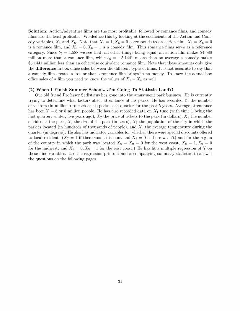
Solution: Action/adventure films are the most profitable, followed by romance films, and comedyfilms are the least profitable. We deduce this by looking at the coefficients of the Action and Com-edy variables, X5 and X6. Note that X5 = 1, X6 = 0 corresponds to an action film, X5 = X6 = 0is a romance film, and X5 = 0, X6 = 1 is a comedy film. Thus romance films serve as a referencecategory. Since b5 = 4.588 we see that, all other things being equal, an action film makes $4.588million more than a romance film, while b6 = −5.1441 means than on average a comedy makes$5.1441 million less than an otherwise equivalent romance film. Note that these amounts only givethe difference in box office sales between the different types of films. It is not accurate to say thata comedy film creates a loss or that a romance film brings in no money. To know the actual boxoffice sales of a film you need to know the values of X1 −X4 as well.

(2) When I Finish Summer School....I’m Going To StatisticsLand?!Our old friend Professor Sadisticus has gone into the amusement park business. He is currently

trying to determine what factors affect attendance at his parks. He has recorded Y, the numberof visitors (in millions) to each of his parks each quarter for the past 5 years. Average attendancehas been Y = 5 or 5 million people. He has also recorded data on X1 time (with time 1 being thefirst quarter, winter, five years ago), X2 the price of tickets to the park (in dollars), X3 the numberof rides at the park, X4 the size of the park (in acres), X5 the population of the city in which thepark is located (in hundreds of thousands of people), and X6 the average temperature during thequarter (in degrees). He also has indicator variables for whether there were special discounts offeredto local residents (X7 = 1 if there was a discount and X7 = 0 if there wasn’t) and for the regionof the country in which the park was located X8 = X9 = 0 for the west coast, X8 = 1, X9 = 0for the midwest, and X8 = 0, X9 = 1 for the east coast.) He has fit a multiple regression of Y onthese nine variables. Use the regression printout and accompanying summary statistics to answerthe questions on the following pages.

31

Correlations:Attendance Price Rides Size

Price -.7Rides .8 .5Size .7 .4 .9Population .7 -.1 .1 .2***************************************************************************The regression equation is

Attendance = 2 + .25Time - .2Price + .01Rides - .001Size + .05Population +.1Temperature + 1Discount -2Midwest - East

Predictor Coef SE Coef T PConstant 2.000 .500 4.00 .0001Time .250 .100 2.50 .0142Price -.200 .050 -4.00 .0001Rides .010 .004 2.50 .0142Size -.001 .002 - .50 .6180Population .050 .025 2.00 .0480Temperature .100 .048 2.08 .0396Discount 1.000 .400 2.50 0142Midwest -2.000 1.000 -2.00 .0480East -1.000 1.000 -1.00 .3196

RMSE = .200 R-Sq = 95.6% R-Sq(adj) = 95.24%


Source DF SS MS F PRegression 9 95.60 10.62 265.5 0.000Residual Error 110 4.40 .04Total 119 100.00

Note: EXCEPT WHERE INDICATED OTHERWISE YOU SHOULD USE α = .05FOR ALL HYPOTHESIS TESTS ON THIS EXAM

(a) Does the model as a whole do a good job of explaining attendance at StatisticsLand parks?Answer this question by performing an appropriate hypothesis test. State the null and alternativehypotheses both mathematically and in words, give the test statistic and p-value, and explain yourreal-world conclusions.

Solution: To test whether the model as a whole is useful we need an overall F test. Our hy-potheses are

32

H0 : β1 = β2 = · · ·β9 = 0–None of time, price, etc. are helpful for explaining the attendence atStatisticsLand parks.HA : At least one βi 6= 0–At least one of time, price, etc. is useful for explaining attendence. Themodel as a whole does a good job of explaining the number of visitors at the theme parks.

Our test statistic is Fobs = 265.5 and the corresponding p-value from the ANOVA table is 0. Sincethis is less than our significance level of α = .05 we reject the null hypothesis. We conclude (notsurprisingly) that at least one of the nine variables does help explain the attendence at the parks.

(b) Does this model do a good job of predicting attendance at StatisticsLand parks? Carefullyjustify your answer.

Solution: To decide whether a model makes good predictions we must look at our typical error,RMSE and compare it to the Y values we are trying to predict. Here RMSE = .2, meaning thatwe typically are off by about 200,000 people when we try to predict the number of visitors to aStatisticsLand park in a given quarter. Since we average Y = 5 or 5 million visitors(c) Give the real-world interpretations of b3 and b7 in this model. Your answer should include theactual numerical values and units as appropriate.

Solution: The coefficient for the Rides variable is b3 = .01. This means for every additional ridethere is at the park, attendance goes up by .01 million = 10,000 people assuming all the othervariables are held fixed. The coefficient for the discount variable is b7 = 1. This tells us that onaverage, when there is a discount being offered 1 million mode people come to the park per quarterthan when there isn’t a discount, assuming all other variables are held fixed.

(d) Based on the correlation table given above the regression printout, should X4, the size of thepark, be a good predictor of attendance? Should it’s coefficient, β4, be positive or negative? Ex-plain briefly in each case.

Solution: The size variable has a quite strong correlation with attendence, Y, so it should by itselfbe a good predictor. Since the correlation is positive we would expect b4 to be positive as well,indicating that as size increases so does attendance. This makes real-world sense. The bigger thepark is the more people it can hold.

(e) Are b4, the estimated regression coefficient for X4, and its p-value consistent with your expec-tations from part (e)? Justify your answer, and, if there is a lack of consistency, say what has gonewrong, giving evidence from the data to support your argument.

Solution: No, the coefficient b4 is negative and it’s p-value of .6180 is well above .05 suggestingthat this variable is not useful WHEN ALL THE OTHER VARIABLES ARE IN THE MODEL.This is probably a multicollinearity issue. From the correlation table we see that Size is also highlycorrelated with the number of rides (.9)–not a surprise since to have a lot of rides you need to havea lot of space! Since the rides variable is more highly correlated with attendance this is the onethat has stayed significant in the model.

33

(f) Does it appear that there are statistically significant differences in park attendance in the threeregions of the country? If so, in which region(s) is attendance the highest? Briefly justify youranswers.

Solution: We need to look at the p-values for the indicator variables for the different regions. TheWest is our reference region. The Midwest indicator has a p-value of .048 meaning attendance thereis significantly different than in the west. From the coefficient of -2 we see that on average atten-dance there is 2 million people lower per quarter. However, the p-value for the East regio is .3196so there is insufficient evidence to show that attendence is different in the East than in the West.Thus we conclude that the West and East have the highest attendence. it appears since East’s coef-ficient is negative that West is the highest but we do not have sufficient evidence to say this for sure.

(g) On average, how much would you expect attendance at a theme park to decrease in a quar-ter if you raised the ticket prices by $5, all other things being equal? Briefly explain your reasoning.

Solution: The coefficient for the price is -.2 meaning that for every extra dollar charged we get adecrease in attendance of 200,000 people, all else being equal. Thus a 5 dollar raise would corre-spond to a loss of 1 million people.

Part i

Find the predicted attendance for the Los Seraphim theme park this summer (that is, summer ofthe first year after the recorded data.) Los Seraphim is a west coast city with a population of 5million people, and an average summer temperature of 70 degrees. You may assume that the parkhas 50 rides, has 50 acres of space, that admission is $45, and that there are currently no discountsbeing offered.

Solution: We just plug into the regression equation being careful of our units. We know the datahas been measured quarterly for 5 years so there have been 20 time points before this year. Summeris the 3rd quarter of the year (winter, spring, summer, fall) so this must be time point 23. Thepopulation is measured in hundreds of thousands of people so we have X5 = 50 for 5 million people.There is no discount offered so X7 = 0 and the park is in the west so X8 = X9 = 0. The rest ofthe numbers can be plugged in as they are given yielding

Y = 2 + .25(23)− .2(45) + .01(50)− .001(50) + .05(50) + .1(70) + 0− 2(0)− 1(0) = 8.7

Thus we predict the park will have 8.7 million customers this summer.

(j) Professor Sadisticus is planning to open a new theme park in the city of Hollybrick. He knowsit will take a while for the park to become profitable but would like to be 95% sure that in totalover the next 10 years attendance will be high enough so that he does not lose money on it. (i)What sort of interval should he use when predicting quarterly attendance at the park to find hisprojected profits over this period? (ii) Do you see any potential problems with the predictions he

34

is making? Briefly explain your reasoning in each case. No calculations are required.

Solution: Prof. Sadisticus should use a confidence interval, not a prediction interval. He isn’tinterested in what happens in one particular quarter–he wants to know on average over the longhaul how much money he will make. The problem with his predictions is that he is extrapolating10 years into the future, way outside the range of his data. There is no guarantee his parks willcontinue to grow at the same rate for such a long time.

(k) Professor Sadisticus has a theory that as it gets hotter more people come to his theme parks.Because of this he is considering adding a new water ride, the Random Splatter, and setting upice-cream stands on hot days, but before the does this he wants to be sure that his theory is correct.Perform the appropriate hypothesis test to prove Professor Sadisticus’ theory. Be sure you stateyour null and alternative hypotheses both mathematically and in words with a justification of yourchoice, give the test statistic and p-value, and explain your real-world conclusions.

Solution: Here we are being asked to do a 1-sided test because he wants to prove as temperaturegoes up attendance goes up. This must be our alternative hypothesis so we have

β6 ≤ 0–Once the other variables have been taken into account terperature has a negative or norelationship with attendance.β6 > 0–After accounting for the other factors, temperature has a positive relationship with atten-dance.

Our test statistric is tobs = 2.08. Since the test is 1-sided we have to divide the p-value from theprintout in half yielding .0198. Since this is less than our significance level of .05 we reject the nullhypothesis and conclude that higher temperatures are associated with higher attendance even afteraccounting for all the other variables.

(l) Silly Sally, a summer intern at StatisticsLand, is very excited by the results of your test in part(j). She concludes that hotter weather causes people to visit your theme parks and proposes thatnew parks should be opened in desert areas like Arizona or Saharan Africa. Explain what is wrongwith (i) Sally’s conclusion and (ii) her proposal. Your answer should include an example of whySally’s conclusion might be wrong.

Solution: Sally is making several mistakes. First, correlation is not necessarily causation. Peoplemay be visiting the parks because it is summer and that is when they are on vacation, not becauseit is hot outside. Her proposal is bad because even if warm weather brought people to the parks,extreme heat as in the desert might not. Models are only useful for making predictions about sit-uations similar to the data on which they were built. Saharan Africa for instance is very differentfrom any of the places in the US that Prof. Sadisticus has his parks and our model will not bereliable there. In fact, probably attendance at parks in such an area would be very low.

35

Biostatistics 201A, Midterm Practice Problems With...

Documents

Transcript of Biostatistics 201A, Midterm Practice Problems With...