Biostat 200 Lecture 8 1. Hypothesis testing recap Hypothesis testing – Choose a null hypothesis,...
55
Biostat 200 Lecture 8 1
-
Upload
virginia-stokes -
Category
Documents
-
view
218 -
download
2
Transcript of Biostat 200 Lecture 8 1. Hypothesis testing recap Hypothesis testing – Choose a null hypothesis,...
Biostat 200 Lecture 8
1

Hypothesis testing recap
• Hypothesis testing– Choose a null hypothesis, one-sided or two sided
test– Set , significance level, to set the probability of a
Type I error ( P(reject H0 | H0 )
– For a given test, a test statistic is calculated, e.g. for a two-sample t-test the test statistic is:
2
11
)()(
212
2121
nns
xxt
p
stat
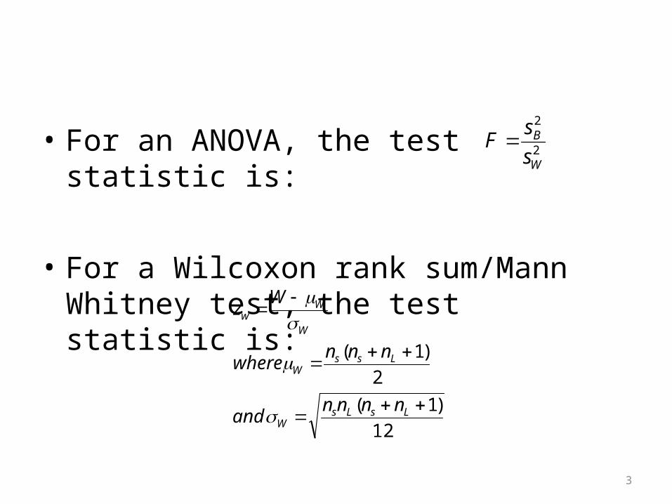
• For an ANOVA, the test statistic is:
• For a Wilcoxon rank sum/Mann Whitney test, the test statistic is:
3
2
2
W
B
s
sF
12
)1(
2
)1(
LsLsW
LssW
W
Ww
nnnnand
nnnwhere
Wz
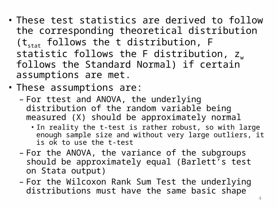
• These test statistics are derived to follow the corresponding theoretical distribution (tstat follows the t distribution, F statistic follows the F distribution, zw follows the Standard Normal) if certain assumptions are met.
• These assumptions are: – For ttest and ANOVA, the underlying distribution of the
random variable being measured (X) should be approximately normal
• In reality the t-test is rather robust, so with large enough sample size and without very large outliers, it is ok to use the t-test
– For the ANOVA, the variance of the subgroups should be approximately equal (Barlett’s test on Stata output)
– For the Wilcoxon Rank Sum Test the underlying distributions must have the same basic shape 4

• One hypothesis test will be “more conservative” than another if that test is less likely to reject the null– A test with a lower level of is more conservative,
e.g. =0.01, sometimes used in clinical trials– A two-sided test is more conservative than a one-
sided test, because even though you are using the same total level, it is divided between the two tails
– If the assumptions of a parametric test are met or are not grossly violated, then a non-parametric test is more conservative than the corresponding parametric test
5

ANOVA and t-test for 2 groups. ttest extot, by( sex)
Two-sample t test with equal variances------------------------------------------------------------------------------ Group | Obs Mean Std. Err. Std. Dev. [95% Conf. Interval]---------+-------------------------------------------------------------------- male | 295 114.9458 7.258138 124.6626 100.6613 129.2303 female | 237 152.1498 11.27012 173.5014 129.9469 174.3527---------+--------------------------------------------------------------------combined | 532 131.5197 6.478136 149.419 118.7938 144.2457---------+-------------------------------------------------------------------- diff | -37.20403 12.94578 -62.63536 -11.77269------------------------------------------------------------------------------ diff = mean(male) - mean(female) t = -2.8738Ho: diff = 0 degrees of freedom = 530
Ha: diff < 0 Ha: diff != 0 Ha: diff > 0 Pr(T < t) = 0.0021 Pr(|T| > |t|) = 0.0042 Pr(T > t) = 0.9979
. oneway extot sex
Analysis of Variance Source SS df MS F Prob > F------------------------------------------------------------------------Between groups 181902.478 1 181902.478 8.26 0.0042 Within groups 11673228.1 530 22024.9586------------------------------------------------------------------------ Total 11855130.5 531 22326.0462
Bartlett's test for equal variances: chi2(1) = 28.7299 Prob>chi2 = 0.0006
When there are 2 groups, the F-statistic equals the t-statistic squared

Wilcoxon rank sum Kruskal Wallis. ranksum extot, by(sex)
Two-sample Wilcoxon rank-sum (Mann-Whitney) test
sex | obs rank sum expected-------------+--------------------------------- male | 295 74838.5 78617.5 female | 237 66939.5 63160.5-------------+--------------------------------- combined | 532 141778 141778
unadjusted variance 3105391.25adjustment for ties -37529.45 ----------adjusted variance 3067861.80
Ho: extot(sex==male) = extot(sex==female) z = -2.158 Prob > |z| = 0.0310
. kwallis extot, by(sex)
Kruskal-Wallis equality-of-populations rank test
+-------------------------+ | sex | Obs | Rank Sum | |--------+-----+----------| | male | 295 | 74838.50 | | female | 237 | 66939.50 | +-------------------------+
chi-squared = 4.599 with 1 d.f.probability = 0.0320
chi-squared with ties = 4.655 with 1 d.f.probability = 0.0310
7
When there are two groups, the chi-square statistic is equal to the z statistic squared (here slightly different because of ties)

More on categorical outcomes
• With the exception of the proportion test, all the previous tests were for comparing continuous outcomes and categorical predictors– E.g., CD4 count by alcohol consumption– Minutes of exercise by sex
• We often have dichotomous outcomes and predictors– E.g. Had at least one cold in the prior 3 months by
sex8
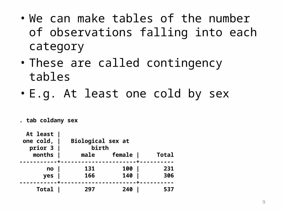
• We can make tables of the number of observations falling into each category
• These are called contingency tables• E.g. At least one cold by sex
. tab coldany sex
At least | one cold, | Biological sex at prior 3 | birth months | male female | Total-----------+----------------------+---------- no | 131 100 | 231 yes | 166 140 | 306 -----------+----------------------+---------- Total | 297 240 | 537
9

Contingency tables• Often summaries of counts of disease versus no disease and
exposed versus not exposed• Frequently 2x2 but can generalize to n x k
– n rows, k columns• Note that Stata sorts on the numeric value, so for 0-1
variables the disease state will be the 2nd row
Exposure
+ - Total
Disease + a b a+b
- c d c+d
Total a+c b+d n=a+b+c+d
Pagano and Gavreau, Chapter 15 10

Contingency tables• Contingency tables
are usually summaries of data that originally looked like this.
Example of data set
Obs. Exposure (1=yes; 0=no)
Disease (1=yes; 0=no)
1 1 1
2 1 0
3 1 1
4 0 0
5 1 1
6 1 0
7 0 0
… … …
n 0 0
Pagano and Gavreau, Chapter 15 11

. list coldany sex
+------------------+
| coldany sex |
|------------------|
1. | yes male |
2. | no male |
3. | yes female |
4. | yes female |
5. | no male |
|------------------|
6. | no male |
7. | no male |
8. | yes male |
9. | yes male |
10. | yes male |
|------------------|
11. | no female |
12. | yes male |
13. | no male |
14. | yes female |
15. | no female |
|------------------|
16. | yes female |
. list coldany sex, nolabel
+---------------+
| coldany sex |
|---------------|
1. | 1 0 |
2. | 0 0 |
3. | 1 1 |
4. | 1 1 |
5. | 0 0 |
|---------------|
6. | 0 0 |
7. | 0 0 |
8. | 1 0 |
9. | 1 0 |
10. | 1 0 |
|---------------|
11. | 0 1 |
12. | 1 0 |
13. | 0 0 |
14. | 1 1 |
15. | 0 1 |
|---------------|
16. | 1 1 |
12

• We want to know whether the incidence of colds varies by gender.
• We could test the null hypothesis that the cumulative incidence of ≥1 cold in males equals that of females. The cumulative incidence is a proportion.
H0: pmales= pfemales HA: pmales≠ pfemales
13

. prtest coldany, by(sex)
Two-sample test of proportion male: Number of obs = 297
female: Number of obs = 240
------------------------------------------------------------------------------
Variable | Mean Std. Err. z P>|z| [95% Conf. Interval]
-------------+----------------------------------------------------------------
male | .5589226 .0288108 .5024545 .6153907
female | .5833333 .0318234 .5209605 .6457061
-------------+----------------------------------------------------------------
diff | -.0244108 .0429278 -.1085476 .0597261
| under Ho: .042973 -0.57 0.570
------------------------------------------------------------------------------
diff = prop(male) - prop(female) z = -0.5680
Ho: diff = 0
Ha: diff < 0 Ha: diff != 0 Ha: diff > 0
Pr(Z < z) = 0.2850 Pr(|Z| < |z|) = 0.5700 Pr(Z > z) = 0.7150
14
• There are other methods to do this (chi-square test)
• Why?– These methods are more general – can be used
when you have more than 2 levels in either variable
• We will start with the 2x2 example however
15

• Overall, the cumulative incidence of least one cold in the prior 3 months is 306/537=.569. This is the marginal probability of having a cold
• There were 297 males and 240 females• Under the null hypothesis, the expected
cumulative incidence in each group is the overall cumulative incidence
• So we would expect 297*.569=169.2 with at least one cold in the males, and 240*.569=136.8 with at least one cold in the females
16
At least | one cold, | Biological sex at prior 3 | birth months | male female | Total-----------+----------------------+---------- no | 131 100 | 231 yes | 166 140 | 306 -----------+----------------------+---------- Total | 297 240 | 537

• We can also calculate the expected number with no colds under the null hypothesis of no difference– Males: 297*(1-.569) = 127.8– Females: 240*(1-.569) = 103.2
• We can make a table of the expected counts
17
Observed data
At least | one cold, | Biological sex at prior 3 | birth months | male female | Total-----------+----------------------+---------- no | 131 100 | 231 yes | 166 140 | 306 -----------+----------------------+---------- Total | 297 240 | 537
EXPECTED COUNTS UNDER THE NULL HYPOTHESIS
At least | one cold, | Biological sex at prior 3 | birth months | male female | Total-----------+----------------------+---------- no | 127.8 103.2 | 231 yes | 169.2 136.8 | 306 -----------+----------------------+---------- Total | 297 240 | 537
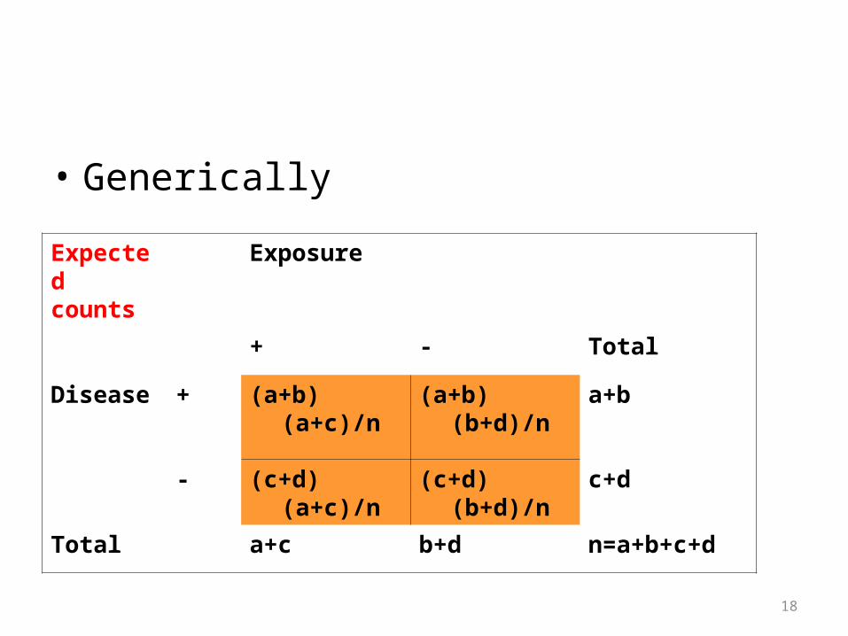
• Generically
18
Expected counts
Exposure
+ - Total
Disease + (a+b)(a+c)/n (a+b)(b+d)/n a+b
- (c+d)(a+c)/n (c+d)(b+d)/n c+d
Total a+c b+d n=a+b+c+d
• The Chi-square test compares the observed frequency (O) in each cell with the expected frequency (E) under the null hypothesis of no difference
• The differences O-E are squared, divided by E, and added up over all the cells
• The sum of this is the test statistic and follows a chi-square distribution
19
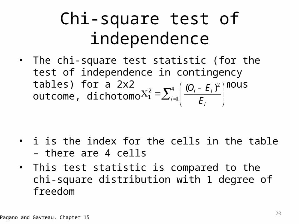
Chi-square test of independence
• The chi-square test statistic (for the test of independence in contingency tables) for a 2x2 table (dichotomous outcome, dichotomous exposure)
• i is the index for the cells in the table – there are 4 cells• This test statistic is compared to the chi-square distribution
with 1 degree of freedom
4
1
221
)(i
i
ii
E
EO
Pagano and Gavreau, Chapter 1520

Chi-square test of independence
• The chi-square test statistic for the test of independence in an nxk contingency table is
• This test statistic is compared to the chi-square distribution• The degrees of freedom for the this test are (n-1)*(k-1), so for
a 2x2 there is 1 degree of freedom– n=the number of rows; k=the number of columns in the nxk table– The chi-square distribution with 1 degree of freedom is actually the
square of a standard normal distribution• Expected cell sizes should all be >1 and <20% should be <5• The Chi-square test is for two sided hypotheses
Pagano and Gavreau, Chapter 1521
nk
ii
iikn E
EO1
22
)1(*)1(
)(
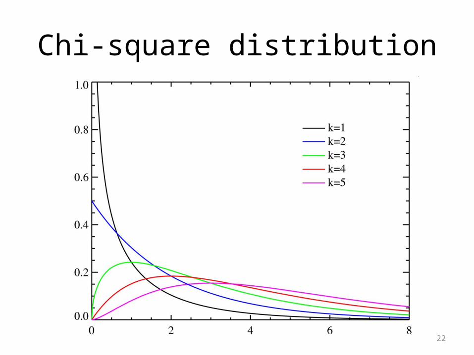
Chi-square distribution
22

Chi-square distribution
23
Chi-square test of independence
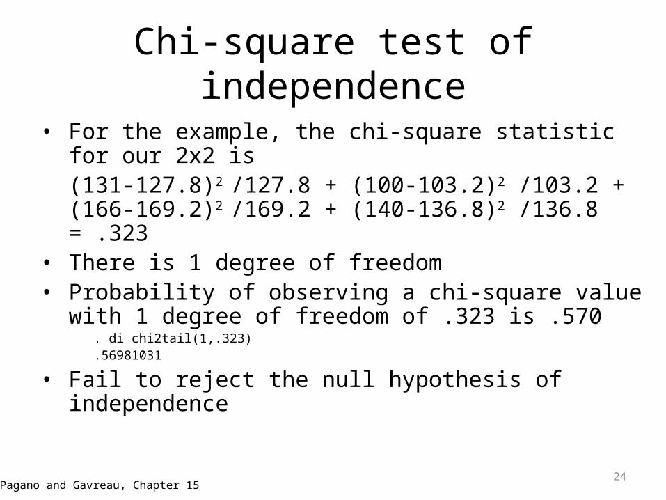
• For the example, the chi-square statistic for our 2x2 is (131-127.8)2 /127.8 + (100-103.2)2 /103.2 + (166-169.2)2 /169.2 + (140-136.8)2 /136.8 = .323
• There is 1 degree of freedom• Probability of observing a chi-square value with 1
degree of freedom of .323 is .570. di chi2tail(1,.323).56981031
• Fail to reject the null hypothesis of independence
Pagano and Gavreau, Chapter 1524

. tab coldany sex, chi
At least |
one cold, | Biological sex at
prior 3 | birth
months | male female | Total
-----------+----------------------+----------
no | 131 100 | 231
yes | 166 140 | 306
-----------+----------------------+----------
Total | 297 240 | 537
Pearson chi2(1) = 0.3227 Pr = 0.570
25
Test statistic (df)p-value
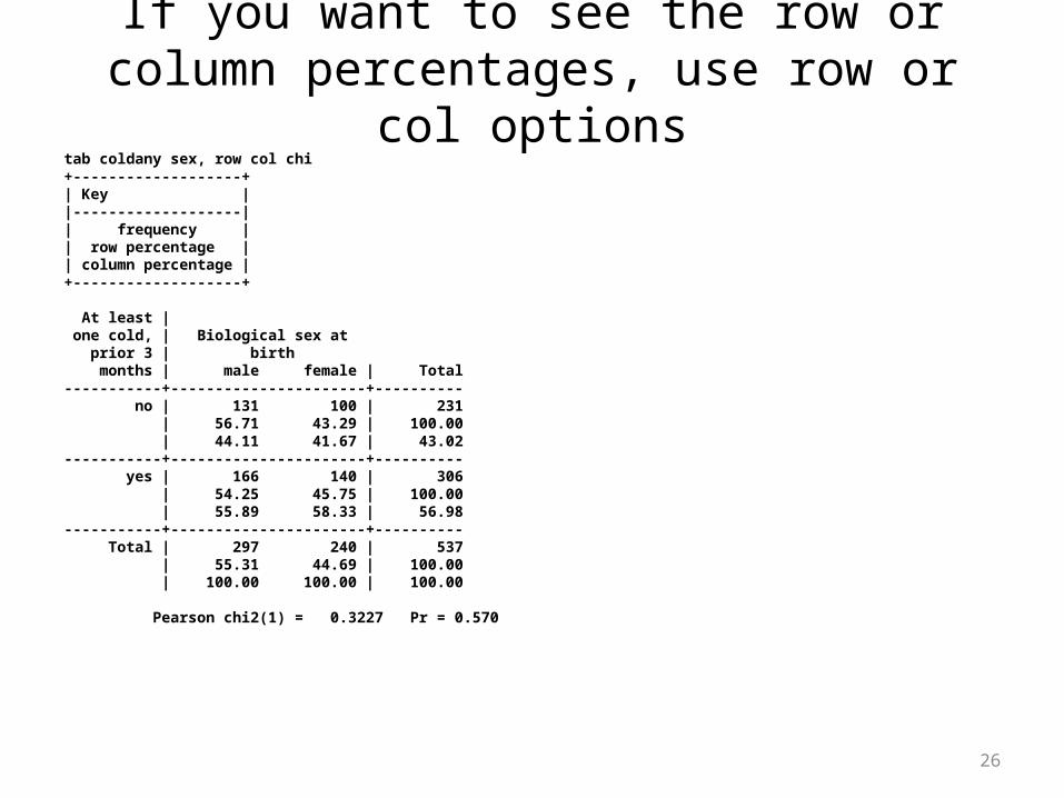
If you want to see the row or column percentages, use row or col options
tab coldany sex, row col chi+-------------------+| Key ||-------------------|| frequency || row percentage || column percentage |+-------------------+
At least | one cold, | Biological sex at prior 3 | birth months | male female | Total-----------+----------------------+---------- no | 131 100 | 231 | 56.71 43.29 | 100.00 | 44.11 41.67 | 43.02 -----------+----------------------+---------- yes | 166 140 | 306 | 54.25 45.75 | 100.00 | 55.89 58.33 | 56.98 -----------+----------------------+---------- Total | 297 240 | 537 | 55.31 44.69 | 100.00 | 100.00 100.00 | 100.00
Pearson chi2(1) = 0.3227 Pr = 0.570
26

• Because we using discrete cell counts to approximate a chi-squared distribution, for 2x2 tables some use the Yates correction
• Not computed in Stata
27
4
1
221
)5.0|(|i
i
ii
E
EO
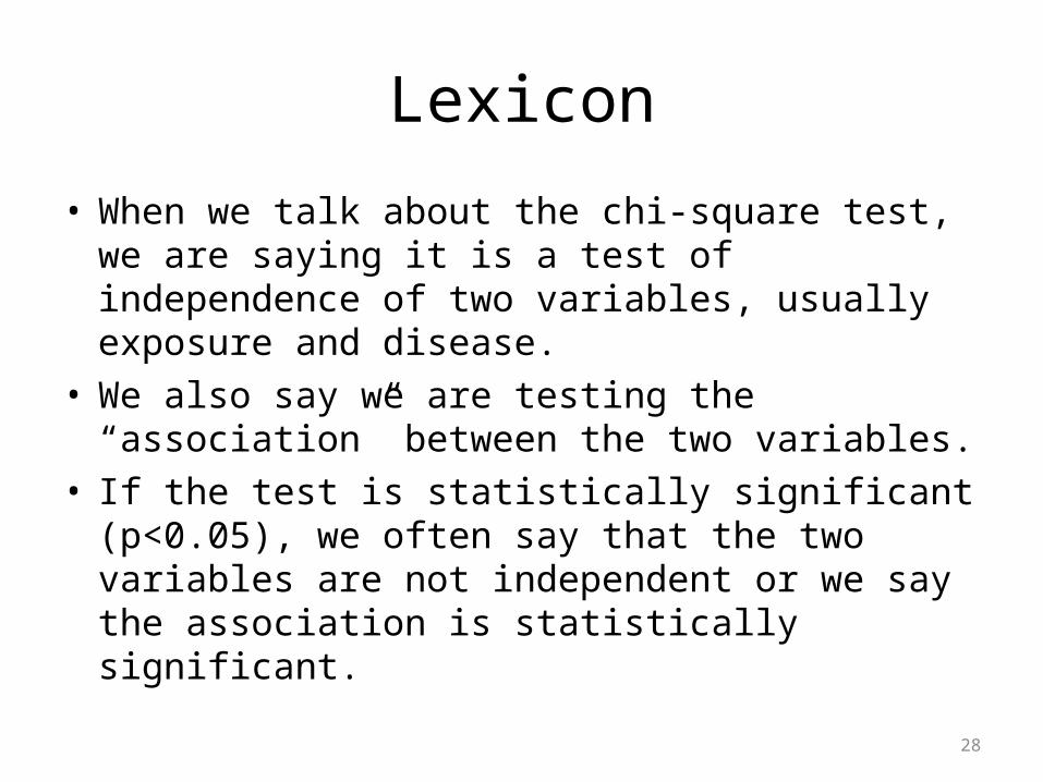
Lexicon
• When we talk about the chi-square test, we are saying it is a test of independence of two variables, usually exposure and disease.
• We also say we are testing the “association” between the two variables.
• If the test is statistically significant (p<0.05), we often say that the two variables are not independent or we say the association is statistically significant.
28

Test of independence• For small cell sizes in 2x2 tables, use the Fisher exact test• It is based on a discrete distribution called the hypergeometric
distribution• For 2x2 tables, you can choose a one-sided or two-sided test
. tab coldany sex, chi exact
At least |
one cold, | Biological sex at
prior 3 | birth
months | male female | Total
-----------+----------------------+----------
no | 131 100 | 231
yes | 166 140 | 306
-----------+----------------------+----------
Total | 297 240 | 537
Pearson chi2(1) = 0.3227 Pr = 0.570
Fisher's exact = 0.599
1-sided Fisher's exact = 0.316
Pagano and Gavreau, Chapter 1529
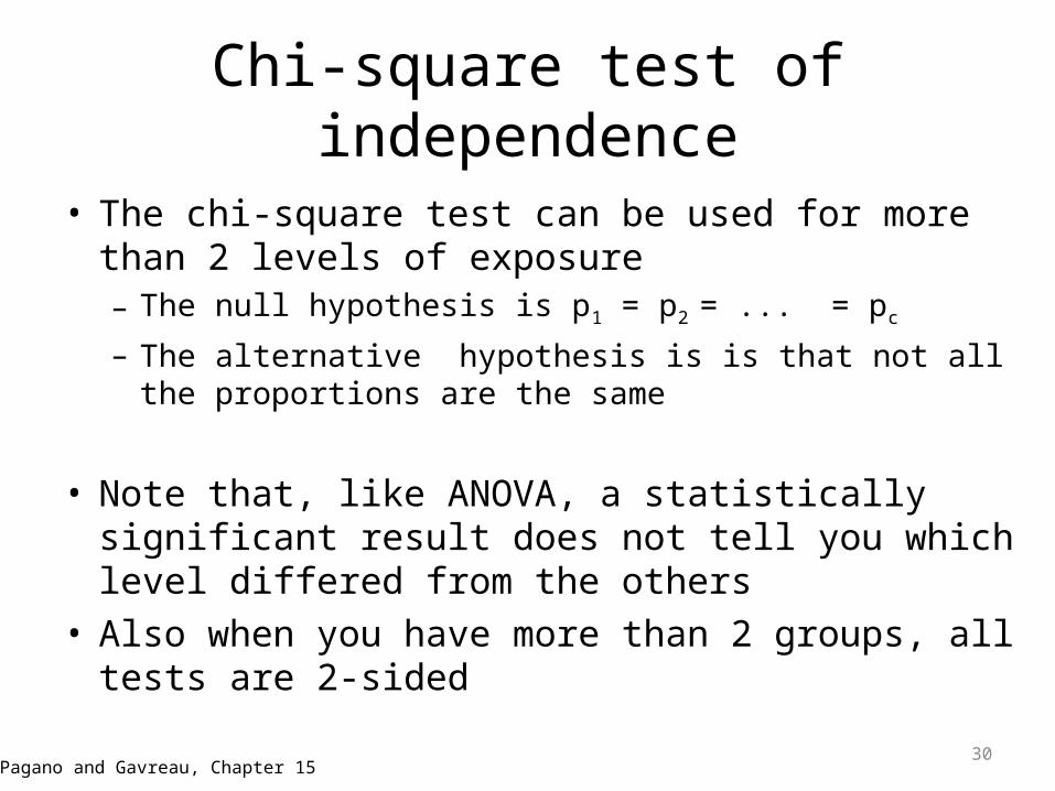
Chi-square test of independence
• The chi-square test can be used for more than 2 levels of exposure– The null hypothesis is p1 = p2 = ... = pc
– The alternative hypothesis is is that not all the proportions are the same
• Note that, like ANOVA, a statistically significant result does not tell you which level differed from the others
• Also when you have more than 2 groups, all tests are 2-sided
Pagano and Gavreau, Chapter 1530

Chi-square test of independence tab coldany racegrp, chi col
+-------------------+| Key ||-------------------|| frequency || column percentage |+-------------------+
At least | one cold, | prior 3 | racegrp months | White, Ca Asian/PI Other | Total-----------+---------------------------------+---------- no | 132 71 30 | 233 | 42.31 44.65 44.12 | 43.23 -----------+---------------------------------+---------- yes | 180 88 38 | 306 | 57.69 55.35 55.88 | 56.77 -----------+---------------------------------+---------- Total | 312 159 68 | 539 | 100.00 100.00 100.00 | 100.00
Pearson chi2(2) = 0.2614 Pr = 0.877
Pagano and Gavreau, Chapter 1531

• Another way to state the null hypothesis for the chi-square test:– Factor A is not associated with Factor B
• The alternative is– Factor A is associated with Factor B
• For more than 2 levels of the outcome variable this would make the most sense
32
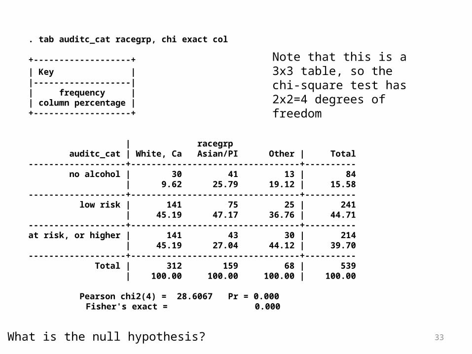
. tab auditc_cat racegrp, chi exact col
+-------------------+
| Key | |-------------------|| frequency || column percentage |+-------------------+
| racegrp auditc_cat | White, Ca Asian/PI Other | Total-------------------+---------------------------------+---------- no alcohol | 30 41 13 | 84 | 9.62 25.79 19.12 | 15.58 -------------------+---------------------------------+---------- low risk | 141 75 25 | 241 | 45.19 47.17 36.76 | 44.71 -------------------+---------------------------------+----------at risk, or higher | 141 43 30 | 214 | 45.19 27.04 44.12 | 39.70 -------------------+---------------------------------+---------- Total | 312 159 68 | 539 | 100.00 100.00 100.00 | 100.00
Pearson chi2(4) = 28.6067 Pr = 0.000 Fisher's exact = 0.000
33
Note that this is a 3x3 table, so the chi-square test has 2x2=4 degrees of freedom
What is the null hypothesis?

Paired data?
• Matched pairs– Matched case-control study– Before and after data
• E.g. Self-reported alcohol consumption before and after being consented for alcohol biomarker specimen collection
34
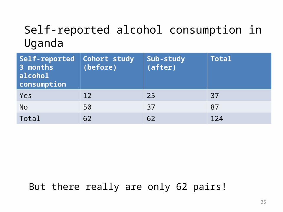
Self-reported 3 months alcohol consumption
Cohort study (before)
Sub-study (after) Total
Yes 12 25 37
No 50 37 87
Total 62 62 124
35
But there really are only 62 pairs!
Self-reported alcohol consumption in Uganda

McNemar’s test – correct table
36
• Null hypothesis: The groups change their self-reported alcohol consumption equally; there is no association between self-reported alcohol consumption and before versus after measures
• The concordant pairs provide no information
After measure Before measure Total
Alcohol consumption prior 3 months Yes No
Yes 12 13 25
No 0 37 37
Total 12 50 62
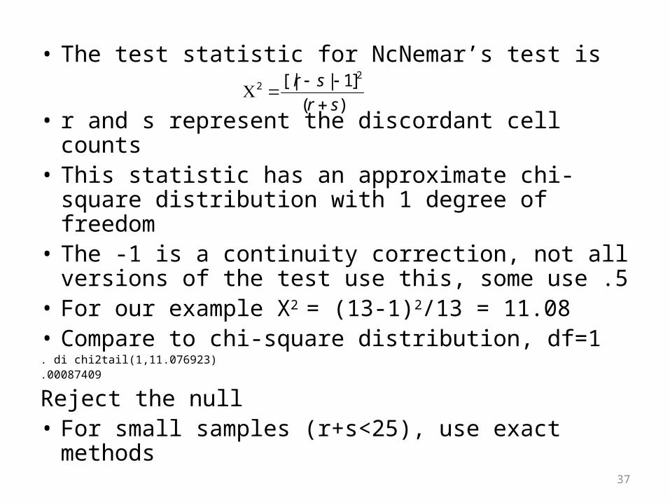
• The test statistic for NcNemar’s test is
• r and s represent the discordant cell counts• This statistic has an approximate chi-square
distribution with 1 degree of freedom• The -1 is a continuity correction, not all versions
of the test use this, some use .5• For our example Χ2 = (13-1)2/13 = 11.08• Compare to chi-square distribution, df=1. di chi2tail(1,11.076923).00087409
Reject the null• For small samples (r+s<25), use exact methods
37
)(
]1|[| 22
sr
sr
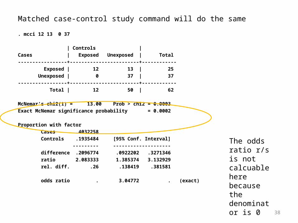
Matched case-control study command will do the same
. mcci 12 13 0 37
| Controls |
Cases | Exposed Unexposed | Total
-----------------+------------------------+------------
Exposed | 12 13 | 25
Unexposed | 0 37 | 37
-----------------+------------------------+------------
Total | 12 50 | 62
McNemar's chi2(1) = 13.00 Prob > chi2 = 0.0003
Exact McNemar significance probability = 0.0002
Proportion with factor
Cases .4032258
Controls .1935484 [95% Conf. Interval]
--------- --------------------
difference .2096774 .0922202 .3271346
ratio 2.083333 1.385374 3.132929
rel. diff. .26 .138419 .381581
odds ratio . 3.04772 . (exact)
38
The odds ratio r/s is not calcuable here because the denominator is 0

Case-control study
39
Controls Total
Cases
Alcohol consumption prior 3 months?
Yes (exposed) No (not exposed)
Yes (exposed) 4 9 13
No (not exposed) 3 11 14
Total 7 20 27
•Cases: Treatment failure: HIV viral load after 6 months of ART >400•Controls: HIV viral load <400Matched on sex, duration on treatment, and treatment regimen class
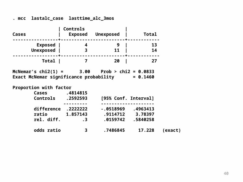
. mcc lastalc_case lasttime_alc_3mos
| Controls |Cases | Exposed Unexposed | Total-----------------+------------------------+------------ Exposed | 4 9 | 13 Unexposed | 3 11 | 14-----------------+------------------------+------------ Total | 7 20 | 27
McNemar's chi2(1) = 3.00 Prob > chi2 = 0.0833Exact McNemar significance probability = 0.1460
Proportion with factor Cases .4814815 Controls .2592593 [95% Conf. Interval] --------- -------------------- difference .2222222 -.0518969 .4963413 ratio 1.857143 .9114712 3.78397 rel. diff. .3 .0159742 .5840258
odds ratio 3 .7486845 17.228 (exact)
40

Comparison of disease frequencies across groups
• The chi-square test is a test of independence• It does not give us an estimate of how much the two
groups differ, i.e. how much the disease outcome varies by the exposure variable
• We use odds ratios (OR) and relative risks (RR) as measures of ratios of disease outcome
• The odds ratio and the relative risk are just two examples of “measures of association”
41

Comparison of disease frequencies – relative risk
Exposure
Disease + - Total
+ a b a+b
- c d c+d
Total a+c b+d n=a+b+c+d
Risk ratio (or relative risk or relative rate) = P (disease | exposed) / P(disease | unexposed)= Re / Ru = a/(a+c) / b/(b+d)
42
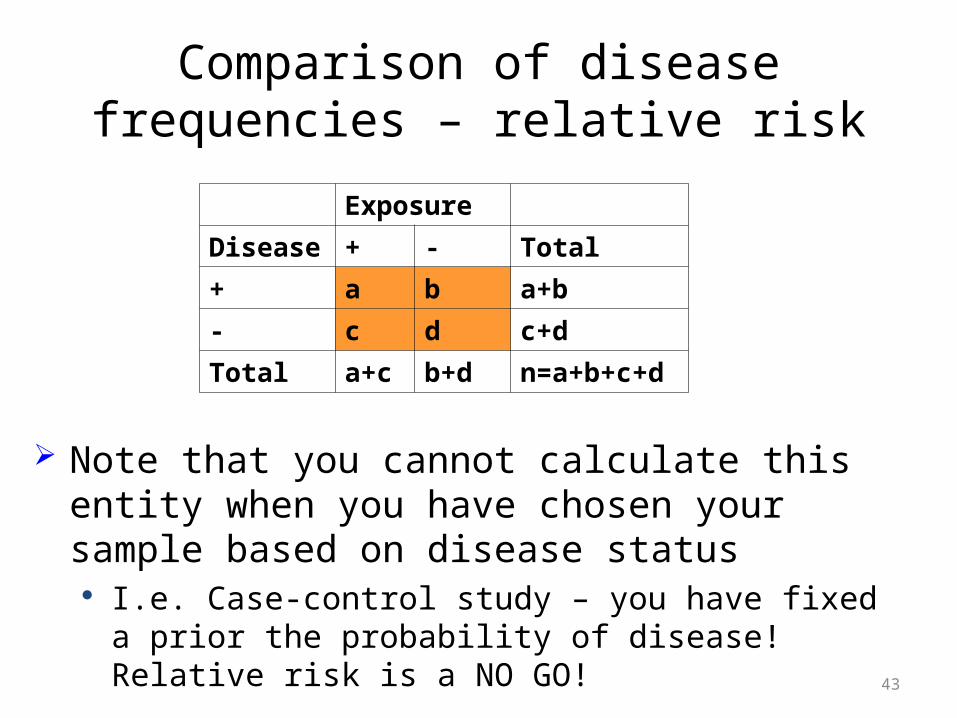
Comparison of disease frequencies – relative risk
Note that you cannot calculate this entity when you have chosen your sample based on disease status
I.e. Case-control study – you have fixed a prior the probability of disease! Relative risk is a NO GO!
Exposure
Disease + - Total
+ a b a+b
- c d c+d
Total a+c b+d n=a+b+c+d
43
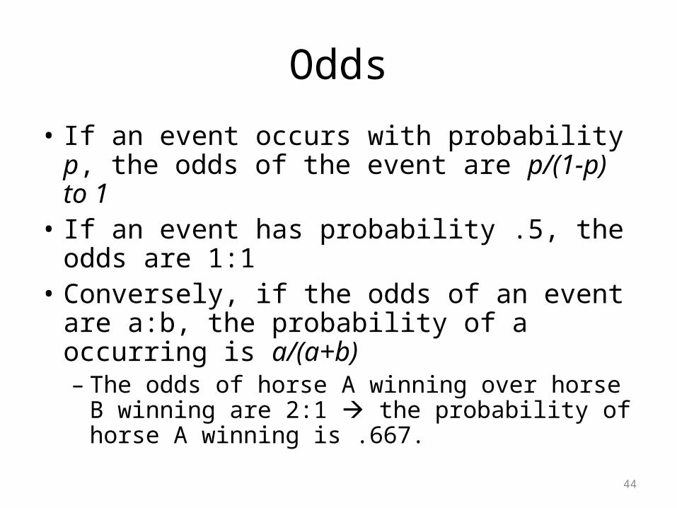
Odds
• If an event occurs with probability p, the odds of the event are p/(1-p) to 1
• If an event has probability .5, the odds are 1:1• Conversely, if the odds of an event are a:b, the
probability of a occurring is a/(a+b)– The odds of horse A winning over horse B winning
are 2:1 the probability of horse A winning is .667.
44

Odds ratio
Odds of disease among the exposed persons = P(disease | exposed) / (1-P(disease | exposed))= [ a / (a + c) ] / [ c / (a + c) ] = a/c
Odds of disease among the unexposed persons = P(disease | unexposed) / (1-P(disease | unexposed))
= [ b / (b + d) ] / [ d / (b + d) ] = b/d Odds ratio = a/c / b/d = ad/bc
Exposure
Disease + - Total
+ a b a+b
- c d c+d
Total a+c b+d n=a+b+c+d
45

Odds ratio note
• Note that the odds ratio is also equal to [ P(exposed | disease)/(1-P(exposed |disease) ] / [ P(exposed | no disease)/(1-P(exposed | no disease) ]
• This is needed for case-control studies in which the proportion with disease is fixed (so you can’t calculate the odds of disease)
46

Interpretation of ORs and RRs
• If the OR or RR equal 1, then there is no effect of exposure on disease.
• If the OR or RR >1 then disease is increased in the presence of exposure. (Risk factor)
• If the OR or RR <1 then disease is decreased in the presence of exposure. (Protective factor)
47
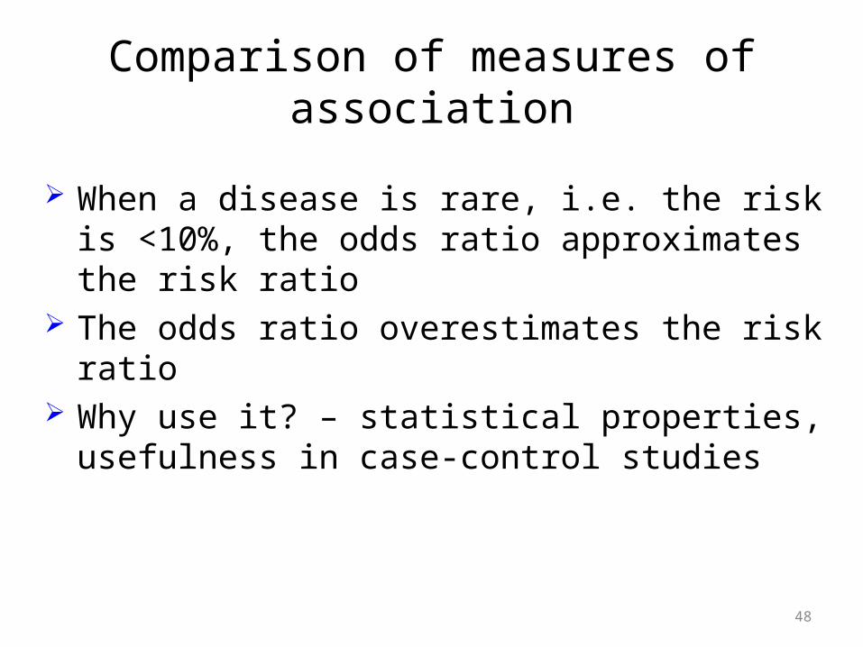
Comparison of measures of association
When a disease is rare, i.e. the risk is <10%, the odds ratio approximates the risk ratio
The odds ratio overestimates the risk ratio Why use it? – statistical properties, usefulness in case-
control studies
48
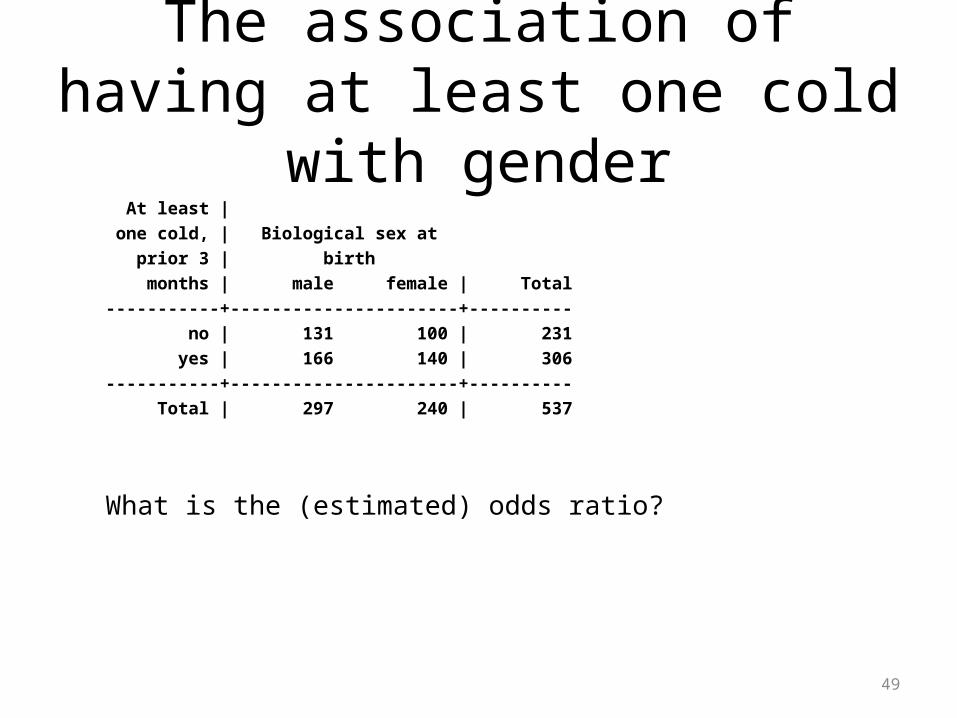
The association of having at least one cold with gender
At least |
one cold, | Biological sex at
prior 3 | birth
months | male female | Total
-----------+----------------------+----------
no | 131 100 | 231
yes | 166 140 | 306
-----------+----------------------+----------
Total | 297 240 | 537
What is the (estimated) odds ratio?
49

95% Confidence interval for an odds ratio
• Remember the 95% confidence interval for a mean µLower Confidence Limit: Upper Confidence Limit:
• The odds ratio is not normally distributed (it ranges from 0 to infinity)– But the natural log (ln) of the odds ratio is approximately normal– The estimate of the standard error of the estimated ln OR is
– This is based on a Taylor series approximation
nX /96.1_
nX /96.1_
dcbaORSE
1111)(ln(
50

95% Confidence interval for an odds ratio
• We calculate the 95% confidence interval for the log odds
• Then exponentiate back to obtain the 95% confidence interval for the OR
51
dcba
ORdcba
OR1111
96.1ln,1111
96.1ln
dcbaOR
dcbaOR
ee1111
96.1ln1111
96.1ln
,
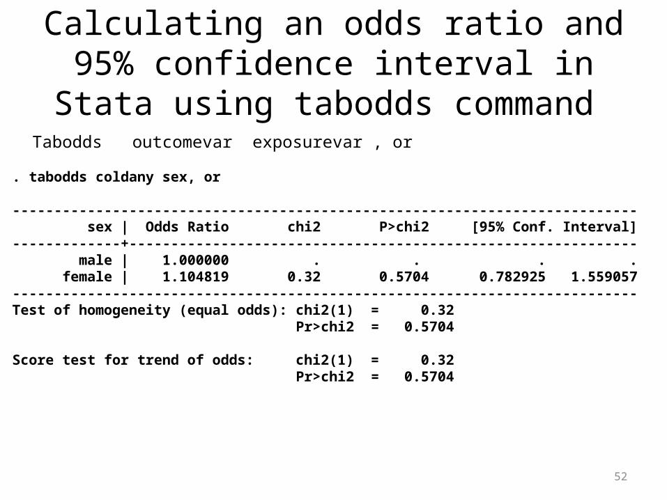
Calculating an odds ratio and 95% confidence interval in Stata using tabodds
command
se ln OR1a
1b
1c
1d
Tabodds outcomevar exposurevar , or
. tabodds coldany sex, or
--------------------------------------------------------------------------- sex | Odds Ratio chi2 P>chi2 [95% Conf. Interval]-------------+------------------------------------------------------------- male | 1.000000 . . . . female | 1.104819 0.32 0.5704 0.782925 1.559057---------------------------------------------------------------------------Test of homogeneity (equal odds): chi2(1) = 0.32 Pr>chi2 = 0.5704
Score test for trend of odds: chi2(1) = 0.32 Pr>chi2 = 0.5704
52

Calculating an odds ratio and 95% confidence interval in Stata using cc
command
se ln OR1a
1b
1c
1d
cc coldany sex Proportion | Exposed Unexposed | Total Exposed-----------------+------------------------+------------------------ Cases | 140 166 | 306 0.4575 Controls | 100 131 | 231 0.4329-----------------+------------------------+------------------------ Total | 240 297 | 537 0.4469 | | | Point estimate | [95% Conf. Interval] |------------------------+------------------------ Odds ratio | 1.104819 | .7719549 1.582124 (exact) Attr. frac. ex. | .0948746 | -.2954124 .3679383 (exact) Attr. frac. pop | .0434067 | +------------------------------------------------- chi2(1) = 0.32 Pr>chi2 = 0.5700
53
Exact confidence intervals use the hypergeometric distribution

Odds ratio for matched pairs
• The odds ratio is r/s• The standard error of ln(OR) is
• So the 95% confidence interval for the estimated OR is
54
rs
srORSE
])(ln[
rs
srOR
rs
srOR
ee96.1ln96.1ln
,

For next time
• Read Pagano and Gauvreau
– Pagano and Gauvreau Chapter 15 (review)– Pagano and Gauvreau Chapter 16