BIOSAND FILTRATION OF HIGH TURBIDITY WATER: MODIFIED FILTER DESIGN AND

SAFE FILTRATE STORAGE

by

Clair Collin

B.E. (Chemical) University of Sydney

Submitted to the Department of Civil and Environmental Engineering in partial fulfilment of the requirements for the degree of

Master of Engineering in Civil and Environmental Engineering

at the MASSACHUSETTS INSTITUTE OF TECHNOLOGY

June 2009

© 2009 Clair Collin. All rights reserved.

The author hereby grants to MIT permission to reproduce and to distribute publicly paper and electronic copies of this thesis document in whole or in part in any medium now known or

hereafter created.

Signature of Author:_____________________________________________________________ Clair Collin

Department of Civil and Environmental Engineering May 15, 2009

Certified by:___________________________________________________________________

Susan Murcott Senior Lecturer of Civil and Environmental Engineering

Thesis Supervisor

Accepted by:___________________________________________________________________ Daniele Veneziano

Chairman, Departmental Committee for Graduate Students

BIOSAND FILTRATION OF HIGH TURBIDITY WATER: MODIFIED FILTER DESIGN AND

SAFE FILTRATE STORAGE by

Clair Collin

Submitted to the Department of Civil and Environmental Engineering on May 15, 2009 in Partial Fulfilment of the Requirements for the Degree of

Master of Engineering in Civil and Environmental Engineering

Abstract Unsafe drinking water is a major cause of water-related diseases that predominantly affect people living in developing countries. The most prevalent water-related disease is diarrhoea, estimated to kill 1.8 million children every year and the second largest cause of childhood death. Today there are many technologies available to treat unsafe water; however, most of these are suited for use with low turbidity source water. The treatment of high turbidity water (>50 NTU) is a challenge that was investigated in this research.

Biosand filters, based on an intermittent slow sand filtration process, are an established household scale water treatment technology widely used in developing countries to treat low turbidity drinking water. This research investigates modifications to the biosand filter design to promote effective pathogen and turbidity reduction in high turbidity water. During field tests conducted in Ghana, a modified biosand filter with dual sand layers for added filtration achieved the greatest pathogen and turbidity removals. This design was then optimised through laboratory studies at MIT.

The dual sand layer biosand filter supports straining and sedimentation of particulate matter from the feed water in a 3-7 cm deep raised upper sand layer prior to biological treatment and further filtration of the water in a 15-16 cm deep lower sand layer. Field testing of the dual sand layer biosand filter showed this filter achieved 59% turbidity reduction, 38% higher than an unmodified control filter; and at least 85% E. coli and 95% total coliform reductions, comparable in performance to unmodified control filters. Laboratory testing demonstrated minimum average reductions of 93% turbidity, 97% E. coli and 71% total coliform after filter maturation, comparable to unmodified control filter results. Dissolved oxygen concentration profiling in the laboratory indicated sufficient oxygen diffused through the upper sand layer to the lower sand layer to support biological activity in the lower sand layer. Recommendations for future studies and design optimisation have been made.

Recontamination of treated water is also a major concern and it is recommended that the biosand filter be used only as required and filtrate collected in a dedicated container with tight fitting lid and tap dispenser.

Thesis Supervisor: Susan Murcott Title: Senior Lecturer of Civil and Environmental Engineering

Acknowledgements I would like to convey my thanks to those who have assisted me to undertake and complete this master’s thesis:

To my supervisor, Susan Murcott, for all of her help and support throughout the year. Thank you for providing me with the opportunity to write this thesis and the opportunity to work on this thesis in Ghana.

To Pure Home Water in Tamale, Ghana, for constructing the biosand filters at the PHW house, helping out with water collection and for supporting the field work conducted as part of this thesis.

To the MIT Ghana team: Sara, Dave and Derek for good times in Ghana and throughout the project.

To all of the MIT CEE 2009 class, Eric, Pete and Susan for making my time at MIT so much fun and run smoothly. I’d like to give special thanks to everyone who helped out with the filters in the MIT laboratory, your help and support is very much appreciated.

Lastly, but certainly not least, thank you to my parents and family for all of their support over the year.

Table of Contents Abbreviations ............................................................................................................................................ 11 1. Introduction ...................................................................................................................................... 13

1.1 Project methodology.................................................................................................................. 13 2 Safe water supply ............................................................................................................................. 15

2.1 Water supply in developing countries ....................................................................................... 15 2.2 Household water treatment and safe storage ............................................................................. 16 2.3 Water supply in Tamale, Ghana ................................................................................................ 17

3. Biosand filtration process ................................................................................................................ 20 3.1 Slow sand filtration process....................................................................................................... 20 3.2 Biosand filtration system........................................................................................................... 21

3.2.1 Biosand filtration process...................................................................................................... 22 3.2.2 Biosand filter design ............................................................................................................. 24 3.2.3 Biosand filter performance.................................................................................................... 27

3.3 Use of the biosand filtration system .......................................................................................... 29 3.3.1 Global biosand filter use ....................................................................................................... 29 3.3.2 Biosand filter use in Tamale, Ghana ..................................................................................... 30

4. Household water storage ................................................................................................................. 32 4.1 Safe water storage...................................................................................................................... 32 4.2 Current household water storage practices ................................................................................ 32

4.2.1 Household water storage in developing countries................................................................. 32 4.2.2 Household water storage in northern Ghana ......................................................................... 33

5. Biosand filter design modification options..................................................................................... 34 5.1 Modified filter design ................................................................................................................ 34

5.1.1 Filtration process ................................................................................................................... 36 5.1.2 Filter filling cycle.................................................................................................................. 38

5.2 Modified BSF set up and operation........................................................................................... 39 5.2.1 Filter set up............................................................................................................................ 39 5.2.2 Filter design modifications.................................................................................................... 40

5.3 Field biosand filter tests and results .......................................................................................... 43 5.3.1 Test procedures ..................................................................................................................... 43 5.3.2 Source (dugout) water quality ............................................................................................... 44 5.3.3 Control filter operation efficiency......................................................................................... 47 5.3.4 Modified filter operation efficiency ...................................................................................... 54

5.4 Recommendations ..................................................................................................................... 62 6. Dual sand layer biosand filter design optimisation ....................................................................... 63

6.1 Dual sand layer BSF design....................................................................................................... 63 6.1.1 Filter cleaning........................................................................................................................ 63 6.1.2 Biological filtration process .................................................................................................. 64 6.1.3 Raised upper sand layer design ............................................................................................. 68

6.2 Dual sand layer BSF set up and operation................................................................................. 69 6.2.1 Filter set up............................................................................................................................ 69 6.2.2 Test procedures ..................................................................................................................... 70 6.2.3 Reproduction of dugout water............................................................................................... 71

6.2.4 Control filter operation efficiency......................................................................................... 73 6.2.5 Filter modifications ............................................................................................................... 74

6.3 BSF optimisation tests and results............................................................................................. 77 6.3.1 Feed water quality ................................................................................................................. 77 6.3.2 Test 1 results ......................................................................................................................... 78 6.3.3 Test 2 results ......................................................................................................................... 86 6.3.4 Test 3 results ......................................................................................................................... 94

6.4 Summary of optimisation test results ...................................................................................... 110 6.5 Discussion................................................................................................................................ 114

6.5.1 DSL BSF performance ........................................................................................................ 114 6.5.2 Estimated cost of DSL BSF ................................................................................................ 115 6.5.3 Recommendations ............................................................................................................... 116

7. Safe Storage for BSF Filtrate ........................................................................................................ 117 7.1 Filtrate quality monitoring in local storage vessels ................................................................. 117 7.2 Field observations of filtrate storage practices ........................................................................ 120 7.3 Safe filtrate storage options ..................................................................................................... 121 7.4 Recommendations for safe filtrate storage .............................................................................. 123

8. Conclusions ..................................................................................................................................... 125 9. References ....................................................................................................................................... 126

Appendix A Water-related diseases commonly found in developing countries Appendix B Test results of International Aid biosand filters in Batamyili Village, Ghana Appendix C Test results of International Aid biosand filters in Zuozugu Village, Ghana Appendix D Biosand filter pore volume calculations Appendix E Solubility of dissolved oxygen in water as a function of temperature

List of Figures Figure 2-1 Improved drinking water coverage 2006.................................................................................. 16 Figure 2-2 Map of Ghana........................................................................................................................... 18 Figure 3-1 Schematic layout of a slow sand filter...................................................................................... 21 Figure 3-2 Schematic layout of a biosand filter ......................................................................................... 22 Figure 3-3 BSFs: a) CAWST design, b) Kanchan™ design, and c) HydrAid filter .................................. 24 Figure 3-4 CAWST style BSF filter layout ............................................................................................... 26 Figure 5-1 Local plastic design biosand filter: design (top) and photo (bottom)....................................... 35 Figure 5-2 Biosand filter with superfine sand layer................................................................................... 37 Figure 5-3 Biosand filter with dual sand layers ......................................................................................... 38 Figure 5-4 Single sand layer biosand filters: a) local plastic design and b) concrete design..................... 39 Figure 5-5 Fuo Mwale, source water dugout ............................................................................................. 40 Figure 5-6 Biosand filter designs tested in Tamale, Ghana ....................................................................... 42 Figure 5-7 Fuo Mwale water turbidity....................................................................................................... 45 Figure 5-8 Fuo Mwale water microbial concentrations ............................................................................. 46 Figure 5-9 Tamale area dugout water quality ............................................................................................ 47 Figure 5-10 BSF filtrate turbidity profile with filtrate volume .................................................................. 49 Figure 5-11 BSF filtrate microbiological profile with filtrate volume....................................................... 49 Figure 5-12 BSF influent and effluent turbidity results, control tests........................................................ 50 Figure 5-13 E. coli counts in BSF influent and effluent, control tests....................................................... 52 Figure 5-14 Total coliform counts in BSF influent and effluent, control tests .......................................... 53 Figure 5-15 BSF influent and effluent turbidity, modified operation ........................................................ 56 Figure 5-16 E. coli counts in BSF influent and effluent, modified operation............................................ 58 Figure 5-17 Total coliform counts in BSF influent and effluent, modified operation ............................... 60 Figure 6-1 Field test dual sand layer biosand filter.................................................................................... 63 Figure 6-2 Oxygen diffusion pathway in a single sand layer BSF ............................................................ 65 Figure 6-3 Oxygen diffusion pathway in a dual sand layer BSF ............................................................... 66 Figure 6-4 Single sand layer biosand filter (BSF A).................................................................................. 74 Figure 6-5 Dual sand layer biosand filter (BSF B) .................................................................................... 75 Figure 6-6 BSF B set-up for dissolved oxygen concentration measurements ........................................... 76 Figure 6-7 DSL BSF upper sand layer and dissolved oxygen measurement ports .................................... 76 Figure 6-8 BSF flow rates, test 1 ............................................................................................................... 79 Figure 6-9 E. coli counts in BSF influent and effluent, test 1.................................................................... 80 Figure 6-10 Total coliform counts in BSF influent and effluent, test 1 ..................................................... 82 Figure 6-11 Dissolved oxygen concentrations at the top of the filters, test 1 ............................................ 84 Figure 6-12 Dissolved oxygen concentrations in the filtrate, test 1........................................................... 85 Figure 6-13 BSF flow rates, test 2 ............................................................................................................. 87 Figure 6-14 Effluent microbiological quality profile with filtrate volume ................................................ 88 Figure 6-15 E. coli counts in BSF influent and effluent, test 2.................................................................. 89 Figure 6-16 Total coliform counts in BSF influent and effluent, test 2 ..................................................... 90 Figure 6-17 Dissolved oxygen concentrations at the top of the filters, test 2 ............................................ 91 Figure 6-18 Dissolved oxygen concentrations in the filtrate, test 2........................................................... 92 Figure 6-19 BSF turbidity, test 3a.............................................................................................................. 95 Figure 6-20 E. coli counts in BSF influent and effluent, test 3a................................................................ 96 Figure 6-21 Total coliform counts in BSF influent and effluent, test 3a ................................................... 98 Figure 6-22 Dissolved oxygen concentrations at the top of the filters, test 3a ........................................ 100 Figure 6-23 Dissolved oxygen concentrations in the filtrate, test 3a ....................................................... 101 Figure 6-24 BSF turbidity, test 3a............................................................................................................ 103 Figure 6-25 E. coli counts in BSF influent and effluent, test 3b.............................................................. 105 Figure 6-26 Total coliform counts in BSF influent and effluent, test 3b ................................................. 107

Figure 6-27 Dissolved oxygen concentrations in the filtrate, test 3b....................................................... 109 Figure 7-1 Jerry cans used for water storage ........................................................................................... 117 Figure 7-2 Jerry can storage turbidity ...................................................................................................... 118 Figure 7-3 Jerry can storage E. coli concentrations ................................................................................. 119 Figure 7-4 Jerry can storage total coliform concentrations...................................................................... 120 Figure 7-5 BSF filtrate collection vessels: a) plastic bucket with lid and b) garawa .............................. 121 Figure 7-6 Community Water Solutions safe water storage bucket ........................................................ 123

List of Tables Table 3-1 Filter specifications of three BSFs: CAWST style, Kanchan™ style and HydrAid™.............. 25 Table 3-2 Biosand filter microbial reductions ........................................................................................... 27 Table 3-3 Biosand filter turbidity reductions ............................................................................................. 28 Table 3-4 BSF performance in Tamale, Ghana ......................................................................................... 31 Table 5-1 BSFs operated in Tamale, Ghana .............................................................................................. 42 Table 5-2 Fuo Mwale water turbidity ........................................................................................................ 44 Table 5-3 Fuo Mwale water microbiological statistics .............................................................................. 46 Table 5-4 BSF flow rates, control tests...................................................................................................... 48 Table 5-5 BSF turbidity removal, control tests.......................................................................................... 51 Table 5-6 BSF E. coli removal efficiency, control tests ............................................................................ 52 Table 5-7 BSF E. coli minimum and maximum removal efficiency, control tests.................................... 53 Table 5-8 BSF total coliform removal efficiency, control tests................................................................. 54 Table 5-9 BSF flow rates, modified design tests ....................................................................................... 55 Table 5-10 Change in flow rate after filter modifications.......................................................................... 55 Table 5-11 BSF turbidity removal, modified design tests ......................................................................... 57 Table 5-12 Change in filtrate turbidity after filter modifications .............................................................. 57 Table 5-13 Average BSF E. coli removal, modified design tests .............................................................. 59 Table 5-14 BSF E. coli minimum and maximum removal efficiency, modified design tests ................... 59 Table 5-15 Average BSF total coliform removal, modified design tests................................................... 61 Table 5-16 BSF total coliform minimum and maximum removal efficiency, modified design tests ........ 61 Table 5-17 Change in filtrate total coliform removal after filter modifications ........................................ 62 Table 6-1 DSL BSF upper sand layer design parameters .......................................................................... 69 Table 6-2 Charles River water quality ....................................................................................................... 71 Table 6-3 BSF flow rate and turbidity removal during control tests ......................................................... 73 Table 6-4 BSF optimisation tests ............................................................................................................... 77 Table 6-5 BSF Feed water characteristics, optimisation study, March 11 to May 4 ................................. 78 Table 6-6 BSF Feed water characteristics, optimisation study, May 4 to May 6 ...................................... 78 Table 6-7 BSF flow rates, test 1................................................................................................................. 79 Table 6-8 BSF E. coli removal efficiency, test 1 ....................................................................................... 81 Table 6-9 BSF E. coli removal efficiency, test 1, theoretical maximum ................................................... 81 Table 6-10 BSF total coliform removal efficiency, test 1.......................................................................... 82 Table 6-11 BSF total coliform removal efficiency, test 1, theoretical maximum...................................... 83 Table 6-12 Change in dissolved oxygen concentrations across the top of the filters, test 1...................... 84 Table 6-13 Change in dissolved oxygen concentrations across the BSF sand layers, test 1...................... 86 Table 6-14 BSF average flow rates, test 2 ................................................................................................. 87 Table 6-15 BSF E. coli removal efficiency, test 2 ..................................................................................... 89 Table 6-16 BSF total coliform removal efficiency, test 2.......................................................................... 90 Table 6-17 Change in dissolved oxygen concentrations across the top of the filters, test 2...................... 92 Table 6-18 Change in dissolved oxygen concentrations across the BSF sand layers, test 2...................... 93 Table 6-19 BSF average flow rates, test 3 ................................................................................................. 94 Table 6-20 BSF turbidity removal efficiency, test 3a ................................................................................ 95 Table 6-21 BSF E. coli removal efficiency, test 3a (old E. coli source).................................................... 97 Table 6-22 BSF E. coli removal efficiency, test 3a (fresh E. coli source)................................................. 97 Table 6-23 BSF total coliform removal efficiency, test 3a (old E. coli source) ........................................ 98 Table 6-24 BSF total coliform removal efficiency, test 3a (fresh E. coli source) ..................................... 99 Table 6-25 Change in DO concentration across the top of the filters, test 3a.......................................... 100 Table 6-26 Change in dissolved oxygen concentration across the BSF sand layers, test 3a ................... 101 Table 6-27 BSF turbidity removal efficiency, test 3b.............................................................................. 103 Table 6-28 Comparison of turbidity removal efficiencies in tests 3a and 3b .......................................... 104

Table 6-29 BSF E. coli removal efficiency, test 3b (old E. coli source).................................................. 105 Table 6-30 BSF E. coli removal efficiency, test 3b (fresh E. coli source)............................................... 106 Table 6-31 E. coli removal efficiencies in tests 3a and 3b (old E. coli source) ....................................... 106 Table 6-32 E. coli removal efficiencies in tests 3a and 3b (fresh E. coli source) .................................... 106 Table 6-33 BSF total coliform removal efficiency, test 3b (old total coliform source)........................... 107 Table 6-34 BSF total coliform removal efficiency, test 3b (fresh total coliform source)........................ 108 Table 6-35 Total coliform removal efficiencies in tests 3a and 3b (old total coliform source) ............... 108 Table 6-36 Total coliform removal efficiencies in tests 3a and 3b (fresh total coliform source) ............ 108 Table 6-37 Change in dissolved oxygen concentrations across the BSF sand layers, test 3b.................. 110 Table 6-38 Comparison of BSF turbidity removal efficiency for the three tests ..................................... 110 Table 6-39 Comparison of BSF E. coli removal efficiency for the three tests ........................................ 111 Table 6-40 Comparison of BSF total coliform removal efficiency for the three tests............................. 111 Table 6-41 Comparison of supernatant dissolved oxygen concentrations for the three tests .................. 112 Table 6-42 Change in dissolved oxygen concentration across DSL BSF upper sand layer .................... 113 Table 6-43 Change in dissolved oxygen concentration across BSF depth of sand.................................. 114 Table 6-44 Comparison of laboratory and field DSL BSF performance ................................................. 115 Table 6-45 Dual sand layer BSF estimated cost ...................................................................................... 115 Table 7-1 Recommendations for safe storage of BSF filtrate.................................................................. 124

Abbreviations Acronyms

BOD Biochemical Oxygen Demand

BSF Biosand Filter

CAWST Centre for Affordable Water and Sanitation Technology

CDC Centers for Disease Control

CEE Civil and Environmental Engineering Department

CWS Community Water Solutions

DO Dissolved Oxygen

DSL BSF Dual Sand Layer Biosand Filter

E. coli Escherichia coli

E.U. European Union

GDWQ World Health Organization Guidelines for Drinking-water Quality

HWTS Household Water Treatment and Safe Storage

JMP Joint Monitoring Programme

LPD BSF Local Plastic Design Biosand Filter

MF Membrane Filtration

MIT Massachusetts Institute of Technology

NGO Non-Government Organisation

PHW Pure Home Water

POU Point-of-Use

SODIS Solar Water Disinfection

TC Total Coliform

UNDP United Nations Development Programme

UNICEF United Nations Children’s Fund

USD United States Dollar

UV Ultraviolet

WHO World Health Organization

Units

atm Atmosphere

CFU Colony Forming Unit(s)

cm Centimetre

kg Kilogram

L Litre

m Metre

mg Milligram

min Minute

mL Millilitre

NTU Nephelometric Turbidity Unit

s second

TU Turbidity Unit

μm Micrometre

13

1. Introduction Facilities for treating drinking water, to render it safe to the consumer, are limited in developing countries, particularly in poor or rural areas and peri-urban slums. As a result, consumption of unsafe drinking water in these areas is common, and can lead to illness, disability and/or death from water-related disease. The most common disease is diarrhoea (including cholera, cryptosporidiosis, giardiasis, and Escherichia coli (E. coli) based diarrhoea, among other causes); other water-related diseases of concern include typhoid, hepatitis, schistosomiasis, trachoma and guinea worm (Cairncross and Feachem, 2003). The provision of appropriate water treatment and safe storage systems, at a municipal- or household-scale, can alleviate the prevalence of these diseases.

The appropriateness of any treatment technology for use in a developing region will be dependent on many factors including raw water quality, cost, education level and community-specific aspects such as local customs, types of water-related diseases present, acceptance and uptake of the technology and its ability to be properly operated and maintained, the availability of water and other environmental and demographic factors (Nath et al., 2006).

The biosand filter (BSF) is an established point-of-use water treatment technology for household use in developing countries. It has been proven to reduce disease-causing pathogens in water; however, the efficacy of the current process is limited to use on raw water with low turbidity. High turbidity water, commonly used as a drinking water source in developing countries, is defined as having turbidity >50 NTU in the Guidelines for Drinking-water Quality (GDWQ), 3rd Edition, 1st Addendum, produced by the World Health Organization (WHO, 2006a), under the description of the roughing filtration process. This study investigated modifications to the biosand filtration process for use in regions where raw water turbidity is high, as well as subsequent safe storage of the filtrate to prevent recontamination.

The research for this project was supported by Pure Home Water (PHW), a non-profit organisation promoting the use of, and disseminating, household water treatment and safe storage systems in Tamale, Ghana. Highly turbid raw water is a concern in this location, which PHW, in collaboration with the Massachusetts Institute of Technology (MIT) Civil and Environmental Engineering Department (CEE), is addressing through research into appropriate water treatment methods. The aim of this present work was to propose a design for a modified BSF with safe filtrate storage, suitable for treating high turbidity water and constructed from locally available materials, which can be distributed by PHW.

1.1 Project methodology This thesis assessed the capacity of various biosand filter designs to remove turbidity and microbial contamination from drinking water sources. The research undertaken as part of this thesis involved the following stages:

A literature review was conducted covering the origins of the biosand filter; the filtration process; filter efficiency (water quality and flow rate), operation, set-up and sustainability; global use of the filter and existing modified designs. Safe storage of filtrate was also researched, covering stored water quality, storage practices in developing countries and safe water storage methods.

Field tests of BSF performance were conducted during January 2009 in Tamale, Ghana. Tests involved operation and performance testing of traditional concrete and plastic designs as well as

14

various modified plastic systems. Local water storage methods were observed, and BSF filtrate was stored and tested for water quality. Water quality indicators measured were turbidity, E. coli counts as an indicator organism for faecal contamination and total coliform (TC) counts.

Data analysis of results recorded during the field tests was conducted to calculate filter efficiency and identify filter modifications that led to enhanced performance.

Additional testing of proposed design modifications was conducted in the laboratories at the Massachusetts Institute of Technology (MIT) to optimise the filter design.

Based on the results of the field and laboratory testing, recommendations for design of a biosand filter suitable for use with highly turbid water source and using materials locally available in Tamale were proposed. Safe storage methods for the filtrate have also been identified.

15

2 Safe water supply Access to a regular, safe water supply is defined as a basic human right by the UN Committee on Economic, Social and Cultural Rights (CESCR) under General Comment No.15: The Right to Water (Arts. 11 and 12 of the Covenant) published in 2003. Safe water is critical to protecting and maintaining health (WHO DWG, 2006a) and attaining wider human development goals (UNDP, 2006). In developing countries, unsafe water is considered a greater threat to human security than violent conflict (UNDP, 2006).

In a move to progress development and eradicate poverty, the United Nations set eight Millennium Development Goals (MDG) to meet the needs of the world’s poorest by 2015 (UN, 2008a). Under Goal 7 Environmental Sustainability, Target 31 has been set to “Halve, by 2015, the proportion of people without sustainable access to safe drinking water and sanitation” (UN, 2008a).

The World Health Organization Guidelines for Drinking-water Quality (2006a, 3rd edition, 1st Addendum) define safe drinking water as water that “does not represent any significant risk to health over a lifetime of consumption, including different sensitivities that may occur between life stages… suitable for all usual domestic purposes, including personal hygiene.”

2.1 Water supply in developing countries The World Health Organisation (WHO) and United Nations Children’s Fund (UNICEF) Joint Monitoring Programme for Water Supply and Sanitation (hereafter referred to as the JMP) report Progress on Drinking Water and Sanitation (2008) details global progress towards the MDG target for drinking water and sanitation. In this report it is estimated that 884 million people worldwide (2006 figures) lack access to an improved water source2. Figure 2-1 shows global improved drinking water coverage for 2006. However, an improved drinking water source does not guarantee safe water supply (safe water as defined by the WHO GDWQ, 2006a), as water may contain harmful infectious or toxic substances, or, contamination may occur during transport and storage (JMP, 2004). Therefore, it is likely that there are more people using unsafe water than unimproved drinking water sources (JMP, 2004).

Diseases related to unclean drinking water place a major burden on human health (WHO, 2006a). The WHO attributes 3.2% of global deaths to unsafe water, sanitation and hygiene, of which, over 99.8% occur in developing countries and over 90% are children (Nath et al., 2006). It is thought that more children die from a lack of safe water and a toilet than almost any other cause (UNDP, 2006). Diarrhoea, directly linked to water and sanitation conditions, is the second largest cause of childhood death (preceded by acute respiratory tract infection), killing 1.8 million children every year (UNDP, 2006). The WHO GDWQ (2006a) declares that drinking water quality interventions

1 The WHO refer to this target as Target 10 (WHO, 2009) as does the UN Millennium Development Project (UNMP, 2009), while the UN Development Programme refers to it as 7c (UNDP, 2009). 2 The JMP defines an improved drinking water source as one that is likely to protect the water source from outside contamination. Improved drinking water sources include the following: piped water in dwelling, plot or yard; public tap / stand pipe; tube well / bore hole; protected dug well; protected spring and rainwater collection. Unimproved drinking water sources include: unprotected dug well; unprotected spring; cart with small tank / drum; tanker truck; surface water (river, dam, lake, pond, stream, canal, irrigation channel) and bottled water.

16

can provide significant benefits to health and that every effort should be made to achieve a drinking water quality as safe as practicable.

Figure 2-1 Improved drinking water coverage 2006 (Source: WHO-UNICEF JMP, 2008)

The majority of water-related diseases are the result of microbial contamination of the water by bacteria, viruses, protozoa or other biological material. Faecal contamination (human or animal) of drinking water supplies signifies the greatest microbial risk due to its potential as a source of pathogenic bacteria, viruses and protozoa. Other contaminants commonly known to compromise the quality of drinking water include toxic cyanobacteria, Legionella and other microbial hazards such as guinea worm. (WHO, 2006a) An overview of water-related diseases commonly occurring in developing countries is provided in Appendix A.

Chemical contamination of drinking water, commonly by arsenic or fluoride, is a concern in some regions of the world, particularly where groundwater is used. Radionuclides are another source of drinking water contamination although total exposure is expected to be very small under normal circumstances. Taste, odour and appearance of drinking water can also cause some concern to consumers, however; there may be no direct health effects from these. Concern is raised that consumers may reject safe water on the basis of aesthetic factors in favour of more appealing, but ultimately unsafe water sources. (WHO, 2006a)

2.2 Household water treatment and safe storage In regions where safe water supply is not available or reliable, point-of-use (POU) treatment systems such as household water treatment and safe storage (HWTS) technologies are an effective alternative (Clasen, 2008). Additionally, HWTS can provide safe water more rapidly and affordably that it would take to design, install and deliver a piped community drinking water supply (Nath et al., 2006).

17

A meta-analysis of water, sanitation and hygiene interventions studying diarrhoea morbidity as a health outcome carried out by Fewtrell and Colford (2004) concluded that water quality interventions, specifically POU treatment, reduced diarrhoeal illness levels in developing countries. Common POU HWTS technologies used in developing countries include the following:

• Boiling, thermal microbial deactivation

• Solar Water Disinfection (SODIS), UV radiation microbial deactivation

• Safe Water System, sodium hypochlorite disinfection combined with safe water storage

• NaDCC (sodium dichloroisocyanurate) dosing, chlorine disinfection

• Ceramic filters, filter usually impregnated with silver for its bactericide and viricide properties

• Biosand filters, mechanical and biological filtration through a sand bed

• Flocculation and disinfection systems, particle removal through flocculation combined with disinfection

Of these HWTS technologies, only the system involving a flocculation step is effective for treating water with high turbidity. The most common flocculation/disinfection product available is PuR© produced by Proctor and Gamble with the Centers for Disease Control (CDC). A study conducted in western Kenya using source water 100-1,000 NTU showed drinking water treated with PUR© had a turbidity of 8 NTU compared to 55 NTU using sodium hypochlorite treatment or traditional settling methods (Crump et al., 2005). Currently 60 million sachets of PUR© are produced each year which will increase to 160 million sachets per year in June 2009 (Allgood, 2008). Each PUR© sachet costs 10 US cents and is capable of treating 10 litres of water (CDC, 2009a). For many people living on less than a dollar a day in the developing world, this represents a significant and ongoing expense.

It is estimated there were 18.8 million people using HWTS (excluding boiling and emergency HWTS product use) in 2007, less than 2% of people without access to an improved drinking water source. The use of HWTS has seen an annual growth rate of 15% over the last three years, although other than boiling, no HWTS product has yet to reach scale in its coverage. (Clasen, 2008)

2.3 Water supply in Tamale, Ghana Tamale is the capital of Northern Region, Ghana (Figure 2-2), a developing country located in sub-Saharan Africa. The population is estimated to be 23 million (CIA, 2009), of which, 45% live below the poverty line, defined as earning less than 1 US dollar per day (WHO, 2006b). It is ranked 142 out of 179 countries on the UN Human Development Index for 2008 under the classification “medium human development.” The climate in the north of Ghana is characterised as hot and dry (CIA, 2009) with a distinct rainy season between June/July and November and a distinct dry season for the remainder of the year.

18

Figure 2-2 Map of Ghana (Source: CIA World Factbook, 2009)

The 2008 JMP reports that 90% of urban-dwelling Ghanaians and 71% of rural Ghanaians have access to improved drinking water sources (2006 data). However, this data is overly optimistic when one considers that water supply service in urban Ghana is, for many people, intermittent, with service only provided some days per week or month, rarely 24 hours a day, 7 days a week. Similarly, rural improved water supplies are frequently located more than 30 minutes walk from the user’s home, requiring frequent water hauling trips, typically by women and children. The Northern Region population is predominantly rural. The WHO estimates that the Northern Region has a child under-5 mortality rate between 155 and 180 for every 1,000 live births (2003 data), of which 12% are attributed to diarrhoeal disease (WHO, 2006b). Diarrhoeal illness accounts for 5% of deaths across all age groups in Ghana (WHO, 2006b).

Unimproved water sources prevalent in the Tamale region include unprotected dug wells (also known as dugouts), cartage and tanker truck deliveries. Particular water quality risks identified in the region include poor microbial quality in all, and high turbidity in most, unimproved water sources. Previous studies in the area have indicated that dugout turbidity can range from 23 to >2,000 TU in the rainy season (Foran, 2007), equivalent to >2,700 NTU (Kikkawa, 2008), to <10 to >800 NTU in the dry season (Johnson, 2007; Yazdani, 2007). As part of this study, dry season turbidity levels were recorded in eight dugouts, with results ranging from 22 to 203 NTU. Turbidity, fine suspended materials which range in size from colloidal to coarse dispersions, is also an indirect measure of microbial count (Reynolds and Richards, 1996). During January 2009, microbial counts (as E. coli) in dugouts ranged from >10 CFU/100mL to 4,000 CFU/100mL (data collected for this study).

HWTS technologies used in the Tamale region to treat water collected from unimproved sources include ceramic filters, biosand filters, cloth filters, flocculation products (alum) and chlorine disinfection products (NaDCC). English company Biwater International together with the Ghana Water Company Limited recently undertook expansion and rehabilitation of the Tamale Water

19

Supply system (Biwater, 2009), providing improved drinking water to new parts of Tamale and outlying communities and improved service to existing parts of the system. Water sampling of Biwater reticulated supplies at the PHW office and in Kpanvo village, Tamale, undertaken in January 2009 as part of this study indicated it was free from microbial contamination (as E. coli) and low turbidity (1 NTU).

20

3. Biosand filtration process Biosand filtration is a point-of-use (POU) water treatment technology widely used in developing countries to improve drinking water quality. The BSF is a modification of slow sand filtration, a biological treatment process, which was established more than two hundred years ago.

3.1 Slow sand filtration process Slow sand filtration (SSF) is a gravity-fed, continuous water treatment process that was established in Scotland in 1804 by John Gibb. The basic process design, on which slow sand filters are still based today, was developed by James Simpson for the Chelsea Water Company in London, England, in 1829. (AWWA, 1991)

Slow sand filtration is a mechanical and biological process of water purification. In the book Slow Sand Filtration (1974) produced by the World Health Organization, authors Huisman and Wood (1974) note that “slow sand filtration is undoubtedly the simplest and most efficient method of treatment for many types of surface water.”

The SSF process works by passing raw water through a sand filter bed, where it is purified. The typical hydraulic loading rate is between 0.1-0.2 m/hour (AWWA, 1991). The raw water initially enters a water reservoir resting above the top sand layer, where it remains for three to twelve hours. During this time heavier suspended particles will begin to settle and lighter particles will begin to coalesce (Huisman and Wood, 1974). The water then passes through the filter where algae and other organic material from the raw water form a thin slimy zoogloeal layer on the sand at the filter surface (Huisman and Wood, 1974), known as the schmutzdecke from the German for “sludge blanket” (AWWA, 1991).

The schmutzdecke is extremely active consuming dead algae and living bacteria from the raw water and converting them to inorganic salts. Simultaneously, nitrogen is oxidised and a significant proportion of inert suspended particles are mechanically strained from the raw water. (Huisman and Wood, 1974)

As the water passes deeper into the filter, beyond the schmutzdecke, a sticky zoogloeal mass of microorganisms, bacteria, bacteriophages, rotifers and protozoa, known as the biofilm, forms and coats the sand particles. Organisms in the biofilm feed on adsorbed impurities and other organic material (including each other) carried by the raw water, and which becomes attached to the sand through mass attraction or electrical forces of attraction. The organic matter is broken down into inorganic matter such as water, carbon dioxide, nitrates, phosphates and similar salts that are removed by the flowing water. (Huisman and Wood, 1974)

A schematic layout of a slow sand filter is provided in Figure 3-1, adapted from the AWWA Manual of Design for Slow Sand Filtration (1991).

No other single process can affect such an improvement in the physical, chemical and bacteriological quality of normal surface waters as that accomplished by biological treatment.

-Huisman and Wood, 1974

21

Figure 3-1 Schematic layout of a slow sand filter

Starting as a clean filter, the biologically active portion of the filter is built up gradually as the microbial population grows and the sand colonises. Bacterial removal in the water is low at the outset as the biological layers build through a process known as ripening (AWWA, 1991). Filter bed ripening may take up to several months, depending on the nutrient concentration of the raw water (AWWA, 1991) and the water temperature (Buzunis, 1995). Upon ripening the biological layers will be fully functioning at which point 2-log to 4-log reductions in biological matter entering with the feed water can be achieved (AWWA, 1991). A 0.8-log to 1.5-log reduction in turbidity was documented by Rachwal et al. (1996); however an upper raw water limit of 30-35 NTU is recommended by the AWWA (1991). The applicability of SSF to treat highly turbid waters is dependent on the use of pre-treatment to reduce levels of turbidity to those mentioned above (AWWA, 1991) and/or the requirement of very frequent filter cleaning.

The filter is operated at a low hydraulic loading rate to allow sufficient contact time between the raw water and the biological layers and to prevent scouring of the schmutzdecke and the biofilm from the sand grains (Buzunis, 1995). Due to the low hydraulic loading rate of the filtration process, the hydraulic retention time of the raw water is significant and a large footprint is required. This means that SSF is a very land intensive technology and may not be a suitable system in densely populated, urban or peri urban areas where land is restricted or expensive (Huisman and Wood, 1974).

3.2 Biosand filtration system Biosand filtration (BSF) is a method of slow sand filtration that has been adapted for use where centralised facilities do not exist or have limited reliability/accessibility. The biosand filter was developed by Dr. David Manz at the University of Calgary, Canada, in the early 1990’s by modifying traditional slow sand filtration technology for household use. The size reduction for household scale water treatment has meant that the hydraulic loading rate, 0.6 m/hour, is much higher than for SSF (Lukacs, 2001). Additionally, the BSF has been designed for intermittent operation as opposed to the continuous operation of the SSF, as is fitting for filter use in the household. A schematic layout of a biosand filter is provided in Figure 3-2.

Raw water

Supernatant

Sand

Gravel

Drainage

Schmutzdecke

Filtrate

Outlet structure

22

Figure 3-2 Schematic layout of a biosand filter

3.2.1 Biosand filtration process The BSF has two main stages of operation, the filling phase and the pause phase. During the filling phase raw water is poured into the filter, pushing water already in the filter out through the drainage pipe work from where it is collected for use. The pause phase occurs between filling cycles during which time a standing layer of water, also referred to as the supernatant, is maintained above the sand bed to feed the system microbiology. System design is based on maximisation of particulate and pathogen removal efficiency from raw water. This is carried out through three main mechanisms of filtration: mechanical filtration, oxidation and natural die-off.

Mechanical Filtration

Mechanical filtration takes place through several different methods in the BSF. Mechanical filtration of particles from the raw water commences with filter start-up.

Straining occurs at the surface of the sand when particles larger than the sand pore size are physically blocked from flowing further during the filling phase. The effective pore size of the sand bed is defined as one-seventh of the diameter of tightly packed spherical sand grains (Huisman and Wood, 1974). Most particles caught in this step are inert matter and parasites (Buzunis, 1995). Typical sand used in BSFs has a grain diameter less than 1 mm (1 mm recommended by Ngai et al. (2006a); 0.7 mm recommended by CAWST (2008)), meaning that particles with diameter greater than 0.14 mm are trapped by straining based on 1 mm diameter.

Sedimentation of particles occurs during the filling and pause phases both at the surface of the sand and onto sand grains within the pores. The efficiency of the sedimentation process is affected by the surface loading rate, that is the water flow rate through the filter, and the particle settling velocity (Huisman and Wood, 1974).

Inertial, centrifugal, Van der Waals, electrostatic and electrokinetic forces of attraction and diffusion all act in the filtration process by drawing contaminant particles into contact with the sand grains (Buzunis, 1995; Huisman and Wood, 1974).

Particles drawn to the sand grains are held in the sand bed by electrostatic forces of attraction, Van der Waals forces and adherence. The adherence mechanism is dependent on the biological activity

Supernatant

Sand

Coarse sand

Gravel

Drainage

Outlet

Lid

Diffuser plate

23

in the sand bed. As the biological layers ripen, organic matter deposited on the sand grains in the upper section of the bed begin to breed and colonise producing the slimy zoogloea (Huisman and Wood, 1974) to which particles in the raw water adhere.

The majority of particles in the raw water are trapped in the schmutzdecke and as more particles build up at the surface, pore size through the filter bed is decreased and a greater amount of contaminants are trapped at the surface (Buzunis, 1995).

Oxidation Filtration

Chemical and microbiological oxidation of organic material and substrates to inorganic salts occurs in both phases of the filter operation. Contaminants that can be easily metabolised are removed during the filling cycle but the majority of contaminants are trapped by the mechanical filtration process and oxidised during the pause cycle via natural predation (Buzunis, 1995). As the trapped particles are oxidised from insoluble organics and substrates to soluble salts, the filter pore size increases again.

As oxidation progresses through the pause phase the dissolved oxygen content of the water decreases and must be replenished. Insufficient oxygen concentration in the water can lead to anaerobic conditions developing causing taste and odour problems in the water. Maintaining oxygen flow to the biologically active layers during the pause cycle to enable the bacteria to metabolise and assimilate the organic matter aerobically is one of the key design elements of the BSF.

Dr. Manz and his team found that oxygen can be supplied to the system during the pause phase by maintaining a standing layer of water, the supernatant, over the sand bed. As oxygen is depleted in the system a dissolved oxygen gradient develops across the depth of the supernatant which drives diffusion of oxygen from the air into the water. Slow convective mixing of the dissolved oxygen in the supernatant enhances oxygen transport to the biolayers, allowing aerobic conditions to be maintained. (Buzunis, 1995)

The supernatant depth must be sufficient to keep the sand bed wet at all times, but shallow enough to allow for adequate oxygen diffusion during the pause cycle. Buzunis (1995) defined 1 mg/L oxygen in the water as the minimum amount of required for biological oxidation to occur. The water depth should also be sufficient to prevent disturbance of the schmutzdecke during the filling phase. An optimal supernatant depth of 5 cm has been established (Ngai et al., 2006a; IDRC, 1998; Buzunis, 1995).

The pause time between filling cycles can affect the efficiency of the oxidation process and should be controlled. As most of the oxidation filtration occurs during the pause phase, sufficient pause time is required for metabolism of the contaminants. A study on the effect of pause time over microbial removal efficiency was carried out by Baumgartner et al. (2007) and showed that greater total coliform removal is achieved with a 12 hour pause time (79.1% removal) compared to a 36 hour pause time (73.7% removal). A minimum of 1 hour is suggested by CAWST in their BSF Manual (2008). A pause time greater than 48 hours can lead consumption of all nutrients in the water and subsequent death of the biologically active layers from lack of food (CAWST, 2008). CAWST (2008) recommend an optimal pause time of six to twelve hours between filling cycles for efficient filter performance.

24

The biologically active zone of the BSF is shallower than in a SSF system resulting from the diffusion limited oxygen availability during the pause phase (Buzunis, 1995). The extent of the biological zone in the BSF is difficult to measure, two estimates are 5 to 10 cm (CAWST, 2008) and 20-40 cm (Buzunis, 1995), as compared to a minimum of 30 to 80 cm for the SSF system (AWWA, 1991). Typical sand bed depth for a BSF is 40 to 50 cm (CAWST, 2008).

The results of oxidation filtration are not immediately seen in the effluent quality. The BSF ripening period occurs after start up and can take from two to three weeks (IDRC, 1998) to 30 days (CAWST, 2008). During this time the bacteria are adhering to the sand grains and proliferating to form the schmutzdecke and biofilm. Until the filter has ripened, performance is sub-optimal and additional filtrate treatment may be required to manage pathogen concentrations.

The efficiency of the oxidation filtration process is also affected by disturbance of the biology. Disturbance typically occurs when the filter is cleaned or moved. Filter cleaning, by stirring the top 1 to 2 cm of supernatant to resuspend settled particles and decanting the dirty water, is required to maintain a sufficient filter flow rate. This method of cleaning is commonly referred to as “swirl and dump” cleaning. Movement of the biolayers during “swirl and dump” cleaning disturbs the system equilibrium, and the biolayer must re-establish before optimal filter performance is achieved again. Re-establishment of the biologically active layers after disturbance often takes several days and up to a week (CAWST, 2008). Movement of the filter should be avoided to prevent disturbance.

Natural die-off

As oxygen is depleted in the schmutzdecke and biofilm during the pause phase, the concentration of dissolved oxygen in the underlying sand becomes too low to support aerobic respiration. Live pathogens that reach this sand depth during the filling cycle typically die-off as a result of the lack of oxygen (Ngai, 2009). Unattached inoculated pathogens will leave the BSF with the effluent.

3.2.2 Biosand filter design Three types of biosand filters were investigated during the research for this thesis: the concrete model designed by CAWST (2008), a plastic model based on the Kanchan™ GEM 505 Arsenic Filter (without modifications for arsenic removal) and the plastic International Aid HydrAid™ model, as shown in Figure 3-3.

Figure 3-3 BSFs: a) CAWST design, b) Kanchan™ design, and c) HydrAid filter (Source: photo a) CAWST, 2006; b) and c) Collin, 2009)

25

Specifications for the three types of biosand filters are compared in Table 3-1. Notable differences in features include the heavy weight of the concrete design and the high cost of the International Aid HydrAid™ filter.

Table 3-1 Filter specifications of three BSFs: CAWST style, Kanchan™ style and HydrAid™

Specification CAWST concrete style1

Kanchan™ plastic style

HydrAid™ plastic style2

Height (m) 0.9 0.53 0.8

Average width (m) 0.3 – 0.4 0.43 0.4

Empty weight (kg) 72 35 4

Filled weight (kg) 160 685 64

Design flow rate (L/hour) 36 15 – 206 47

Fine sand depth (m) 0.4 – 0.5 0.23 0.4 – 0.54,7

Fine sand grain size (mm) <0.7 <18 <14,9

Pore volume (L) 1510 15 – 185 2010

Cost (USD) $12 – 30 $15 – 164,11 $75

1 CAWST Biosand Filter Manual (2008) 2 International Aid (2009) 3 Measured by the author 4 Estimated by Kikkawa (2008) 5 Ngai (2009) 6 Ngai et al. (2006b) 7 Fine sand depth for HydrAid™ filter is sum of fine and superfine (see note 8) sand layer depths. 8 Ngai et al. (2006a) 9 The HydrAid™ filter has an additional 5 cm deep (Kikkawa, 2008) superfine sand layer, diameter

unknown, above the fine sand. 10 Refer to Appendix D for calculations 11 Ngai et al. (2004)

26

Filter set-up

The three filters described above, and most other biosand filters available, are set up similarly and have the same key elements, shown in Figure 3-4 using the CAWST concrete style filter as an example. Common key elements of biosand filter include the following:

• Filter shell, to contain the sand media and water

• Lid, to prevent contaminants from entering the system.

• Diffuser plate, to minimise disturbance of the schmutzdecke during the filling cycle.

• Outlet pipe, to drain water from the bottom of the filter and hydraulically control the top water level of the supernatant.

• Gravel layer, to support the sand. The CAWST (2008) design specifies 12 mm diameter gravel; the Kanchan™ 6 to 15 mm diameter gravel; the International Aid HydrAid™ BSF gravel diameter is unknown.

• Coarse sand layer, to prevent the fine sand from dropping in to the gravel and either leaving the system with the filtered water or clogging the outlet pipe.

• Fine sand layer, which supports the mechanical filtration and provides a surface for the schmutzdecke and biofilm to form on. Properties of this layer are provided in Table 3-1.

• Supernatant, to prevent drying out of, and to facilitate oxygen diffusion to, the biologically active layers.

The International Aid HydrAid™ filter includes a superfine sand layer above the fine sand layer. Kikkawa (2008) estimated the depth of this layer to be 5 cm. Observations made by the author during the installation of HydrAid™ filters in Gbabshie, Ghana, in January 2009, confirmed this as the approximate depth.

Figure 3-4 CAWST style BSF filter layout (Source: CAWST, 2009b)

Outlet

Supernatant

Schmutzdecke

Concrete Shell

27

Filter operation

Raw water is added to the sand filter via a diffuser plate. The water then passes through the schmutzdecke and biofilm layers in the fine sand where it is cleaned. The outlet pipe drains the cleaned water from the bottom of the filter and discharges it for collection and use.

Water that has been retained in the filter during the pause phase, that is to say the pore volume water plus supernatant, undergoes more extensive cleaning due to the longer exposure to sedimentation and adherence mechanisms, oxidation filtration and natural die-off than water that exits the filter in the same filling phase. Therefore, the greater the pore volume of the BSF, the greater the quantity of water that can be withdrawn from the filter with pause phase treatment. But if the volume of water added to the filter in one filling cycle is greater than the pore volume, some of the water may not receive adequate filtration. Pore volumes for the three BSFs investigated are given in Table 3-1.

The filter should be stored away from direct sunlight to prevent algal growth in the system. Children and animals should be kept away from the BSF to prevent damage to the system from hanging off the outlet pipe, knocking the filter and causing disturbance of the biologically active layers or playing with the outlet pipe and contaminating the filtrate. Additionally, filtrate should be stored safely to prevent recontamination (for further details refer to Chapter 4 on safe storage).

When the flow rate stops or slows significantly the filter should be cleaned using the “swirl and dump” method (described in section 3.2.1). In some areas where water has high turbidity, filter manufacturers have recommended cleaning the filter every three days (observations of International Aid HydrAid™ filter installations in Northern Ghana, made by the author).

3.2.3 Biosand filter performance

Water quality

A review of several point-of-use household drinking water treatment technologies by Sobsey et al. was conducted in 2008. A summary of the results for the BSF are provided in Table 3-2.

Table 3-2 Biosand filter microbial reductions

Contaminant Baseline reduction Maximum reduction

Bacteria 1-log 3-log

Viruses 0.5-log 3-log

Protozoa 2-log 4-log

Stauber (2007) conducted a field trial of biosand filters in Bonao, Dominican Republic, and reported a 47% reduction in diarrhoea amongst BSF users in comparison to non-users.

28

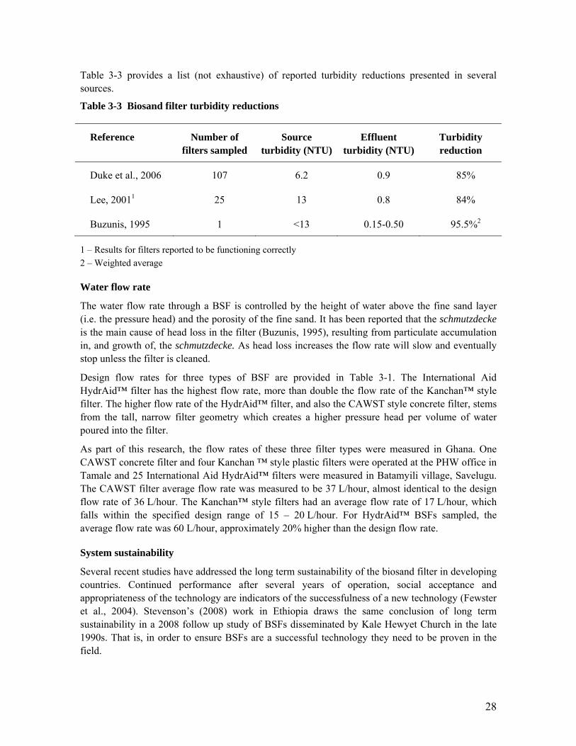
Table 3-3 provides a list (not exhaustive) of reported turbidity reductions presented in several sources.

Table 3-3 Biosand filter turbidity reductions

Reference Number of filters sampled

Source turbidity (NTU)

Effluent turbidity (NTU)

Turbidity reduction

Duke et al., 2006 107 6.2 0.9 85%

Lee, 20011 25 13 0.8 84%

Buzunis, 1995 1 <13 0.15-0.50 95.5%2

1 – Results for filters reported to be functioning correctly 2 – Weighted average

Water flow rate

The water flow rate through a BSF is controlled by the height of water above the fine sand layer (i.e. the pressure head) and the porosity of the fine sand. It has been reported that the schmutzdecke is the main cause of head loss in the filter (Buzunis, 1995), resulting from particulate accumulation in, and growth of, the schmutzdecke. As head loss increases the flow rate will slow and eventually stop unless the filter is cleaned.

Design flow rates for three types of BSF are provided in Table 3-1. The International Aid HydrAid™ filter has the highest flow rate, more than double the flow rate of the Kanchan™ style filter. The higher flow rate of the HydrAid™ filter, and also the CAWST style concrete filter, stems from the tall, narrow filter geometry which creates a higher pressure head per volume of water poured into the filter.

As part of this research, the flow rates of these three filter types were measured in Ghana. One CAWST concrete filter and four Kanchan ™ style plastic filters were operated at the PHW office in Tamale and 25 International Aid HydrAid™ filters were measured in Batamyili village, Savelugu. The CAWST filter average flow rate was measured to be 37 L/hour, almost identical to the design flow rate of 36 L/hour. The Kanchan™ style filters had an average flow rate of 17 L/hour, which falls within the specified design range of 15 – 20 L/hour. For HydrAid™ BSFs sampled, the average flow rate was 60 L/hour, approximately 20% higher than the design flow rate.

System sustainability

Several recent studies have addressed the long term sustainability of the biosand filter in developing countries. Continued performance after several years of operation, social acceptance and appropriateness of the technology are indicators of the successfulness of a new technology (Fewster et al., 2004). Stevenson’s (2008) work in Ethiopia draws the same conclusion of long term sustainability in a 2008 follow up study of BSFs disseminated by Kale Hewyet Church in the late 1990s. That is, in order to ensure BSFs are a successful technology they need to be proven in the field.

29

Sobsey et al. (2008) document the continued use of BSFs in more than 85% of households in Cambodia and the Dominican Republic as long as 8 years after introduction. This was mainly attributed to the robustness of the technology, the simplicity of operation and necessity of a one-time purchase only. They also note that the BSF has a very low breakage rate and a low proportion of BSFs become disused over time.

A study on the sustainability of household BSFS by Fewster et al. (2004) came to a similar conclusion as Sobsey et al. Fewster et al. followed a project by Medair, which introduced BSFs to a rural community in Kenya where more than 2000 units were sold. After fours years of operation, 51 household filters were studied of which more than 70% were producing a water quality below 10 CFU/100mL from raw water containing an average of 462 CFU/100mL. Among those filters where performance was poor, the poor filter performance was correlated to the use of heavily contaminated water with low sand levels and access by children to the filters. A household survey carried out indicated that 97% of filter owners were generally satisfied with the performance of the filter and all owners thought that the filter had been a worthwhile purchase.

Duke et al. (2008) studied BSF performance and use in 107 households in Haiti. The concrete filters had been installed over a five year period with the average filter age being 2.5 years. Filter use was discontinued in only two households. No broken filters were observed although four were clogged and subsequently cleaned. Surveys indicate that one hundred percent of households liked the filter, citing better water quality (49%), health protection (22%) and “because it works well” (7%). Additionally, all households said the filter was easy to use. 99% of households reported that the filtrate appeared cleaner and tasted and smelled better than the raw water, and that the filter produced sufficient water for the household. 95% of households indicated they thought their family’s health had improved since using the filter, while 5% did not notice a change in health. 95% of households also responded that they would recommend the filter to others.

3.3 Use of the biosand filtration system

3.3.1 Global biosand filter use It is currently estimated that there are more than 270,000 BSFs successfully installed around the world (Nichols, 2008), predominantly in Asia, Africa and South America.

The largest disseminators of BSFs are the following non-government organisations:

• CAWST, a Canadian NGO that trains organisations to build concrete BSFs among other HWTS

• Samaritans Purse Canada, charitable provision of the concrete BSF worldwide

• BushProof, a social enterprise marketing concrete BSFs in Africa

• HAGAR, a social enterprise marketing concrete BSFs in Cambodia

• International Aid, disseminating a licensed plastic BSF

• Rotary clubs, dissemination concrete or plastic BSFs

In 2003 a BSF was successfully designed by Tommy Ngai of the Massachusetts Institute of Technology, USA, and Sophie Walewijk of Stanford University, USA, to remove arsenic in addition to pathogens from drinking water in Nepal. The design incorporates a top layer of 5 kg iron

30

nails, locally available in Nepal, which rust upon contact with the raw water. The arsenic sorbs onto the rust which then detaches from the nails and flows through the BSF with the water (Ngai and Walewijk, 2003). The sand filters out the arsenic rich rust, removing most of the arsenic from the water. Overall, the filter removes an average of 85 – 90% arsenic, 90 – 95% iron 85 – 99% total coliforms and 80 – 95% turbidity (Ngai et al., 2007). The filter, known as the Kanchan™ Arsenic Filter, is available for sale in Nepal, is undergoing technology verification under the Government of Bangladesh’s Environmental Technology Verification process and is being pilot tested under an Asian Development Bank grant in Cambodia (Murcott, 2008). To date, 10,000 Kanchan Arsenic Filters have been sold, reaching an estimated 100,000 people in Nepal (Murcott, 2008).

3.3.2 Biosand filter use in Tamale, Ghana Just as BSFs have been adapted to address arsenic in South East Asia, studies are currently underway in Tamale and the greater Northern Region, Ghana, to adapt the BSF to the highly turbid raw water sourced from dugouts. During the January 2009 dry season, dugout turbidity values for eight dugouts ranged from 22 NTU to 203 NTU, with and average of 100 NTU (tested by the author). However, turbidity values as high as 800 NTU (Johnson, 2007; Yazdani, 2007) have been recorded in the dry season and as high as 2,700 NTU in the rainy season (Foran, 2007). These high turbidity values need to be considered in the design and operation of a BSF if the technology is going to be considered for dissemination in this region. To date there is limited research available on the performance of the BSF under Ghanaian Northern Region conditions, especially with respect to the high turbidity in the water.

Kikkawa (2008) tested Kanchan™ style plastic BSFs, referred to as local plastic design (LPD) BSFs, for implementation in the region. She constructed the filters entirely from locally available materials, with shells and piping constructed from plastic. The aim of her research was to compare the Kanchan™ style set up with one sand layer to a modified design with two separate sand layers. Four filters were tested and compared: two modified BSFs, one with an additional 5 cm deep sand layer and one with an additional 10 cm deep sand layer, and two unmodified single sand layer BSFs. Filter maturation occurred at day 13 of operation, after which 92-95% turbidity removal was recorded for all four BSFs. The two modified BSFs showed slightly higher turbidity removal, attributed to either their potential to withstand greater operational variation or the requirement for less frequent cleaning. On day 11 of operation, 80 – 90% removal of total coliforms was recorded from an average 12,000 total coliform CFU/100 mL influent.

During 2007, the Non Government Organisation (NGO) International Aid distributed 200 plastic HydrAid™ brand BSFs to local village Kpanvo. Performance of 30 of these filters was tested by Kikkawa (2008). The raw water was found to have an average turbidity of 32 NTU and the effluent 2.9 NTU, a turbidity reduction of 87%. The average total coliform count in the filtered water was 420 CFU/100mL, which was recorded as 95% removal efficiency. Kikkawa recommended further testing of the HydrAid™ filters using raw water with higher turbidity insofar as the average turbidity of the Kpanvo filters was substantially below the average raw dugout water quality in the area detailed above. The author of this thesis visited Kpanvo in January 2009 and found that recent connection to reticulated water supplies had meant that the BSFs were no longer in use in the village.

Approximately 100 International Aid HydrAid™ BSFs were distributed in Batamyili village, in Savelugu to the north of Tamale, by the E.U./UNICEF Integrated Water, Sanitation and Hygiene (I-

31

WASH) Project in late 2008. 25 of these filters were randomly sampled as part of this thesis research in January 2009 for turbidity, E. coli and total coliform removal efficiency. The average feed turbidity was 25 NTU, and the filtrate 5 NTU, representing an average 80% removal efficiency. The E. coli reduction capacity of the filters averaged 65%, with influent average quality 399 E. coli CFU/100 mL and filtrate average 69 E. coli CFU/100 mL. An average of 55% total coliform reduction was observed, with average influent concentration 10,165 total coliform CFU/100 mL and average filtrate quality 3,340 total coliform CFU/100 mL. Further water quality details are provided in Appendix B.

During January 2009, Zuozugu village which had also received International Aid HydrAid™ BSFs was visited as part of this study. Four BSFs which had been in operation for approximately three months were tested. The average feed turbidity to the filters was 162 NTU and the average filtrate 39 NTU, a 76% average reduction capacity. The E. coli tests showed an average influent concentration of 250 E. coli CFU/100 mL was reduced by 89% to an average of 32 E. coli CFU/100 mL in the filtrate. On average, 72% of total coliform counts were reduced from 6,800 total coliform CFU/100 mL average in the influent to 3,580 total coliform CFU/100 mL in the filtrate. Additional details on the water quality can be found in Appendix C.

The performance of the local plastic design BSFs tested by Kikkawa (2008) and data for the HydrAid™ BSFs are summarised in Table 3-4.

Table 3-4 BSF performance in Tamale, Ghana

Parameter LPD BSF HydrAid™, Kpanvo

HydrAid™, Batamyili

HydrAid™, Zuozugu

Turbidity reduction

92 – 95% 87% 80% 76%

E. coli reduction N/A N/A 65% 89%

Total coliform reduction

80 – 90% 95% 55% 72%

32

4. Household water storage Safe storage of filtered water is paramount to maintaining the quality of treated water, and therefore the health benefits that can be achieved through the biosand filtration process. Ensuring that safe storage practices and technologies are implemented as part of BSF operation is critical to the success and sustainability of the filter.

4.1 Safe water storage Unhygienic handling of water during transport or within the home can contaminate previously safe water (JMP, 2008). In particular, pathogens of faecal origin often recontaminate water that is initially of an acceptable microbiological quality when unhygienic handling practices are carried out (WHO, 2008).

Dedicated use of an appropriate safe water storage vessel, independent of the vessel used to collect raw water, is critical for effectively maintaining water quality. It is also important that the safe storage container be adequately capped or covered to protect the water from contamination, primarily from contact with hands or utensils as well as dust, animals, birds and insects (CDC, 2001). Such contaminant access can be limited by the use of a tight fitting lid only opened during vessel filling or decanting (Stevenson, 2008), a narrow opening for filling and a tap or spigot for dispensing (WHO, 2008).

In the early 2000s, the United States Centers for Disease Control and Prevention (CDC) was promoting a strict definition of safe storage as discussed in the 2001 guidelines “Safe Water Systems for the Developing World: A Handbook for Implementing Household-Based Water Treatment and Safe Storage Projects.” More recently, the CDC is advocating safe water storage in plastic containers with a narrow mouth, lid and spigot (CDC, 2009b) that are locally available, or modifications of containers that are locally available including wide-mouthed containers that have a fitted lid (CDC, 2008).

4.2 Current household water storage practices

4.2.1 Household water storage in developing countries Typical water storage containers in developing countries include plastic or metal buckets, 55 gallon oil drums, wide-mouthed clay pots, cooking pots, pitchers and thermoses. In many developing countries clay pots are the traditional, and favoured, container for water storage (CDC, 2001), however, these present a risk for recontamination of the water through contact with hands or unhygienic utensils to retrieve water (Ogutu et al., 2001).

Changes in microbiological water quality from the source to the household are typically attributed to two factors: indicator bacteria die-off and further contamination in transit, storage or handling. Indicator bacteria die-off can occur if there is competition for oxygen or nutrients in the water, causing a decrease in bacteria concentration. Further contamination of the water can come from dipping dirty hands and utensils in the water (Wright et al., 2004; Jensen et al., 2002) or the use of a contaminated storage vessel and results in increased bacterial counts. In their review of studies comparing source water and household stored water microbiological qualities (total coliforms, faecal thermo-tolerant coliforms and E. coli) in developing countries, Wright et al. (2004) found that most observational studies indicated water quality degraded after collection. Furthermore, the

33

decline in microbiological water quality at the household was proportionally greater for relatively uncontaminated source water, such as water from an improved source. Similarly, in a study carried out by Jensen et al. (2002) in Pakistan comparing the microbiological quality of source and household stored water, it was observed that increased microbiological contamination occurred in the household when source water contained less than 100 E. coli CFU/100 mL, whereas a net bacterial die-off was recorded in the stored household water when E. coli in the source water was greater than 100 E. coli CFU/100 mL.

Jensen et al. (2002) also compared the stored microbiological water quality of traditional wide-necked ceramic storage vessels to modified narrow-necked ceramic vessels that limited access to hands and cups. They found that for high E. coli counts (greater than 200 E. coli CFU/100 mL) there was no difference between the performance of the two vessels, however, for source water with lower E. coli counts the narrow-necked vessel produced a significantly better stored water quality.

In their study of 107 Haitian households with BSFs Duke et al. (2006) found that 3% of filtrate samples taken at the BSF outlet were contaminated with >10 E. coli CFU/100 mL. Stored filtrate was then analysed and it was reported that 22% of the samples had >10 E. coli CFU/100 mL, a notable increase in the number of samples contaminated by unsafe storage.

4.2.2 Household water storage in northern Ghana In northern Ghana water is typically collected from a dugout, communal pump or communal standpipe in a jerry can or metal pail (locally known as a garawa). At the household, water is transferred from the collection vessel to an outdoor clay storage container. Some natural sedimentation occurs inside the clay pots, as observed by the layer of mud at the bottom of many clay storage pots and by simple sedimentation studies carried out by Doyle in 2008. Water is taken directly from the clay pot if no water treatment system is in place, or decanted with a cup or calabash from storage to treatment in the case of the ceramic pot filter, or poured directly into the upper diffuser basin the case of a BSF.

During the visit to Batamyili village, Savelugu, Ghana, the quality of raw water stored in 25 traditional clays pots was sampled and compared to the water quality in the local source water dugout. The turbidity of the dugout was measured to be 46 NTU and water decanted from a typical storage pot averaged 25 NTU, lower than the source water suggesting settling had occurred in the storage pot. The E. coli concentration of the dugout was in the range 10-99 NTU/100 mL, as was the water in 60% of the storage pots. Another 28% of the storage pots were found to have E. coli concentrations between 100-300 NTU/100 mL, and the remainder had concentrations >700 CFU/100 mL, indicating significant contamination had occurred during storage. The total coliform concentration of the dugout was 2,700 CFU/100 mL. Only 3 of the 25 storage pots had a total coliform count lower than the source water. The average total coliform concentration was found to be 10,165 CFU/100 mL, much higher than the source water.

Green (2008) assessed water storage practices in the same northern Ghana study area and found a significant short term need for low cost plastic storage containers. She also concluded that a commercial market would exist for these containers.

34

5. Biosand filter design modification options This research investigated options to modify the BSF such that it can be used to improve the quality of highly turbid source water. The design process involved two main steps:

1. Development of several design options, field testing of designs and selection of one design for further testing. This step is presented in this chapter.

2. Optimisation of selected design based on theoretical calculations and laboratory testing, which is presented in chapter 6.

This first stage of the design process involved theorising design modifications that could improve the capability of the biosand filter to operate under high turbidity raw water levels whilst maintaining its pathogen reduction ability. The design options were then tested in Tamale and the results assessed to identify which design modifications achieved the greatest improvement in water quality. Tests were carried out in two phases:

a. Unmodified filters operated as control filters to give baseline performance data to enable comparison of the different filters and comparison of filters pre- and post-modification.

b. Testing of modified filters and performance evaluation.

It was also desirable that the BSF be entirely constructed of materials that are commonly and locally available in developing countries in order to render the design transferable to regions other than Tamale. Using local materials also promotes system sustainability through local equipment purchasing, which in turn supports the economy and creates a technology that can be maintained and repaired locally. Only simply constructed and easy-to-operate modified BSFs were considered as feasible options for use in developing countries.

5.1 Modified filter design The focus of the design modification options was to reduce the turbidity of the raw water. In turn, this would reduce the pathogen concentration in the water through mechanical straining of biological particles and allow increased oxidation filtration to occur by removing particles which can hinder contact, and therefore reactions, between the biologically active layers and the incoming organic material.

The biosand filters detailed in this research were the Kanchan™ style local plastic design (LPD) BSFs constructed by Kikkawa in 2008, shown in Figure 5-1, however the supernatant depth was increased to 5 cm for this research from the 4 cm used by Kikkawa.

35

Figure 5-1 Local plastic design biosand filter: design (top) and photo (bottom) (Source: Collin, 2009)

Diffuser Plate 14cm deep

41cm

Lid

Outlet

Underdrain 33cm

Freeboard 15.5 cm

Supernatant 5 cm

Fine Sand (<1 mm) 18 cm

Gravel (6 - 15 mm) 5 cm

Coarse Sand (3 - 6 mm) 3.5 cm

36

5.1.1 Filtration process Standard simple processes for turbidity reduction in drinking water sources include the following:

• Sedimentation

• Coagulation and flocculation

• Filtration

Sedimentation

Sedimentation can be a relatively slow process, as it is dictated by the terminal velocity of the particle (as defined by Stoke’s law3). Therefore the extent of sedimentation achieved is dependent on the length of time the water is allowed to stand and the raw water quality. Considering one of the key features of the BSF is the fast flow rate of filtered water, the addition of a sedimentation process to the BSF as part of this modified design was considered to be cumbersome and likely to detract from the value of the filter.

Moreover, many people in the Tamale region already practise sedimentation by storing water collected from dugouts and other unimproved sources in large clay pots and decanting water from the top as required. If a sedimentation stage were to be included in the BSF, the benefits are likely to be minimal as the water has already passed through an initial sedimentation step.

Overall, the inclusion of an exclusive sedimentation step was not considered to be a feasible option in this research.

Coagulation and Flocculation

Sometimes when surface waters are excessively turbid, coagulation and flocculation is practised in the Tamale area with alum at a household scale. The coagulation process involves rapid mixing of the alum into the raw water to increase collisions between the alum and particles causing particle destabilisation. Flocs then form between the destabilised particles and rapidly settle.

Adding a coagulation and flocculation step integral to the BSF is likely to cause disturbance to the biological layers due to the requirement for rapid mixing. Settling of large flocs in the system could cause it to clog. As a separate step, alum dosing will increase the complexity of the system and the amount of equipment required (pots etc.).

Adding alum dosing to the process represents an ongoing cost to the people, which, in addition to the capital cost of the BSF, could create a system too expensive for many people to purchase or maintain.

Moringa4 can also be used as a coagulant, either purchased commercially or collected and prepared at a household scale. As with alum, the purchase of Moringa is considered to be cost prohibitive for many people; and household production is likely to be too time-consuming, and possibly complex, for reliable widespread use.

3 Stoke’s law gives the terminal velocity of the particle based on calculation of gravitational and drag force for laminar flow conditions (Metcalf and Eddy, 2004). 4 Moringa oleifera, commonly known as Moringa, is a tree widely found in West Africa and other parts of the world, the seeds of which can be used as a coagulant in coagulation-flocculation and sedimentation processes.

37

Neither alum nor Moringa dosing were considered to be feasible options in this research.

Filtration

The BSF is a filtration system and modifications to the existing filtration process were considered to be the most feasible design alternatives to the single sand layer BSF. In her study, Kikkawa (2008) analysed several methods of filtration that could be included as part of the BSF to reduce turbidity, as follows:

Roughing filtration. This involves slowly passing water through several metres of gravel packed in a vessel such as a pipe. Turbidity is removed in a similar fashion to slow sand filtration, yet is less effective due to the large gravel size and hence comparatively smaller surface area. Given the amount of media required, the size of the filter and the similar operating mechanism, Kikkawa ruled out roughing filtration as an option and subsequently it was not considered as a feasible option in this research.

Use of smaller diameter sand grains for the fine sand layer. Decreasing the mean sand grain diameter in the fine sand layer would decrease the mean pore size and therefore increase the amount of particles mechanically strained; and increase the sand surface area enabling a more extensive growth of the biolayer and hence more oxidation filtration. Concerns about increased clogging frequency and the cost of finer sand led Kikkawa to eliminate this as an option.

However, while the use of finer grains for the entire depth of the sand layer was considered to be unfeasible, this research did investigate the potential for increased turbidity removal using a combination of <1 mm sand grains in the fine sand layer with a 5 cm deep layer of <0.7 mm superfine sand grains on top. The concept of this filter is outlined in Figure 5-2.

Figure 5-2 Biosand filter with superfine sand layer

Gravel (6-15 mm) 5 cm Coarse Sand (3-6 mm) 3.5 cm

Fine Sand (<1 mm) 11.5 cm

Supernatant 5 cm

Freeboard 17 cm

Superfine Sand (<0.7 mm) 5 cm

Diffuser plate

38

Addition of a second, separate sand layer. This is the dual sand layer BSF design option favoured and studied by Kikkawa (for details of the study refer to Modification of a Biosand Filter in the Northern Regions of Ghana by Kikkawa 2008). By passing the raw water through a raised upper sand layer, then through the supernatant (4 cm deep in Kikkawa’s design) and subsequent sand layer, Kikkawa attempted to create a second, separate biolayer to increase the amount of treatment. Depths of 5 cm and 10 cm were investigated for the raised upper sand layer. During the overnight pause phase the upper sand layer was removed from the BSF and stored in source (dugout) water. Kikkawa’s modified LPD BSF with two sand layers showed 2 – 3% increased turbidity removal compared to two single sand layer LPD BSFs operated simultaneously to control results from the two modified BSFs. As the upper layer of sand was moved everyday and then placed in a basin of water (creating a backflow of water through the sand) it is suspected that the reason for poor improved performance of the dual sand layer BSFs over the control BSFs was caused by disturbance to any additional biological activity by the water flow. It is likely only mechanical filtration was occurring in the raised upper sand layer.

The research carried out for this thesis built on Kikkawa’s design modification of using two sand layers. The main change in the dual sand layer BSF design for this thesis was to integrate the raised upper sand layer as a permanent feature of the BSF, as shown in Figure 5-3. A 6 cm deep raised upper sand layer was used to provide mechanical filtration only, not oxidation filtration.

Figure 5-3 Biosand filter with dual sand layers

5.1.2 Filter filling cycle As discussed in Section 3.2.1 most of the oxidation filtration in the system occurs during the pause phase of filter operation. The pore volume of the Kanchan™ style LPD BSF is estimated to be 15 – 18 L (Ngai, 2009), however, during set up of Kanchan™ style BSFs in the MIT laboratory in

Diffuser plate

Diffuser plate supporting upper

sand layer

Gravel (6-15 mm) 5 cm Coarse Sand (3-6 mm) 3.5 cm

Fine Sand (<1 mm) 16.5 cm

Supernatant 5 cm Freeboard 2 cm

Water layer 3 cm

Fine Sand (<1 mm) 6 cm Coarse Sand (3-6 mm) 1 cm

Raised upper sand layer

Lower sand layer

39

December 2008 as part of this research, the pore volume of the filter was recorded as 10 L (refer to section 6.2.1).

Assuming a pore volume of 10 L for the LPD BSFs, it was decided to fill the filters with 10 L of water each filling cycle, using one 20 L jerry can of water per two filters. To monitor the effluent quality of water which passed through the filter in one filling phase, without remaining for the pause phase, one out of the five experimental LPD BSF units was selected to be operated as a single sand layer BSF filled with 20 L water each filling cycle, twice the amount of the other filters and double the pore volume of an LPD BSF.

In summary, the design modifications tested as part of this field-based research were the addition of a superfine sand (<0.7 mm) layer, the addition of a second separated fine sand layer (<1 mm grain diameter) and the operation of one filter fed twice the volume of water (20 L) of the other filters.

5.2 Modified BSF set up and operation

5.2.1 Filter set up On December 11, 2008, five BSFs were set up by staff at the Pure Home Water office in Tamale, Ghana. The filters were constructed for use as single sand layer filters for low turbidity water by staff that had participated in a BSF training program run by CAWST in Tamale, Ghana, several months prior to this set up.

Four of the BSFs were reconstructions of the Kanchan™ style LPD BSFs used by Kikkawa in January 2008 but without the design modifications she studied. The fifth was a concrete BSF, the concrete shell of which was donated by the Community Life Improvement Programme (CLIP), and had been constructed during a CAWST training session held in November 2008. Diagrams of the LPD BSF and the concrete BSF are provided in Figure 5-4.

Figure 5-4 Single sand layer biosand filters: a) local plastic design and b) concrete design (Source: concrete filter from CAWST 2009b)

Diffuser Plate 14cm deep

41cm Lid

Outlet

33cm

Supernatant

Fine Sand (<1 mm)

Gravel (6 - 15 mm)

3.5 cm

26.4 cm

22cm 39 cm

25 cm

Outlet

18 cm

46 cm

Coarse Sand (3 - 6 mm) 5 cm

5 cm 5 cm

5 cm

5 cm 15.5 cm

Supernatant

Fine Sand

40

From December 11 through to January 8, 2009 the five filters were filled daily with 10 L of water from Fuo Mwale (see Figure 5-5), a dugout located approximately two kilometres from the PHW office. Dugout water was collected daily by PHW staff and/or the author in 20 L plastic jerry cans which are typical vessels for water collection in this area and in many developing regions. The water was then poured into a 50 L bucket to enable the water to be gently poured into the BSFs, mimicking the storage and filter feeding conditions from clay storage pots by locals.

Figure 5-5 Fuo Mwale, source water dugout (Source: Collin, 2009)

The intention of filling the filters for a four week period before the arrival of the author was to enable filter ripening to occur. This allowed observations of matured filter efficiency by the author from the outset of the field visit. It also meant that biological activity had been established in the sand media so that the filter would return to mature operation more rapidly after disruptive design modifications were made as compared to a new filter.

The filters were kept in the PHW office backyard in full shade provided by a mat hut structure expressly built for the purpose of protecting them from UV light which can cause algal growth in the filter and disturb the filtration processes.

From January 8, to January 15, 2009, inclusive, the single sand layer filters were run under the operating conditions started by the PHW staff as control filters against which the modified filters would be compared. Commencing January 16, 2009 modifications were made to the filters.

5.2.2 Filter design modifications The following section describes the modifications made to some of the filters starting January 16, 2009. The filters were operated and data collected up to and including January 23, 2009. The plastic

41

BSFs were numbered 1 through to 4, and the concrete one lettered C. Figure 5-6 provides an overview of the filter layouts studied in this stage of the investigation and corresponds to the filter descriptions given below.

BSF 1

This filter was kept as a single sand layer BSF as was constructed by the PHW staff, as shown in Figure 5-4a. BSF 1 used to investigate the influence of filling cycle volume on effluent quality, as described in section 5.1.2. Each day the filter was filled with water to the top of the container freeboard and topped up until 20 L of water had been added.

BSF 2

BSF 2, the dual sand layer BSF, was modified to include a raised upper sand layer (<1 mm), separated by a layer of water from the lower sand layer, as shown in Figure 5-3. Based on the freeboard of the filter, a 6 cm deep layer of sand was chosen, similar to the 5 cm deep layer used by Kikkawa (2008). The filter was not high enough to set up a 10 cm sand layer.

The upper sand layer was added to the existing diffuser plate, separated by a 1 cm layer of coarse sand (3-6 mm) to prevent the fine sand falling through or clogging the holes in the diffuser plate. A new 5 cm deep supernatant layer was created above the upper sand layer by extending the outlet pipe work 14.5 cm. The additional sand was taken from BSF 3 as it was biologically active sand to assist BSF 2 to ripen following the modification process. During the transfer from BSF 3 to BSF 2 the sand was placed in dugout water to maintain the biology. The remaining freeboard in BSF 2 was reduced to 2 cm.

Due to difficulties in construction, modifications to this filter were completed on January 18; the filter was fed on January 16 and 17 to maintain the biological activity.

BSF 3

This filter, the superfine sand layer BSF, was used to test the effects of adding a superfine sand (<0.7 mm) layer on top of the fine (<1 mm) layer, as shown in Figure 5-2. The top 5 cm of fine sand were removed (and re-used in BSF 2). New sand was sourced locally, sieved to <0.7 mm and washed three times in dugout water to remove suspended particles and other free contaminants. On January 16 the superfine sand layer was added to BSF 3.

BSF 4

This filter was run as a control single sand layer BSF, used for comparing the performance of the modified BSFs. Figure 5-4a shows the filter set up in detail, as was constructed by the PHW staff. No design modifications were made and it was operated under the same 10 L water per day flow regime as BSFs 2, 3 and C.

BSF C

BSF C was a concrete filter with set up shown in Figure 5-4b, operated under the same flow regime as BSFs 2-4. This filter was used to compare performance of the plastic filters against one of concrete construction.

Table 5-1 summarises the design and operating conditions of the five BSFs used in the field studies of modified filter designs conducted in Tamale, Ghana.

42

Table 5-1 BSFs operated in Tamale, Ghana

Biosand Filter Identification

Design Filling regime

BSF 1 Single sand layer Double volume (20 L/day)

BSF 2 Dual sand layer, incorporating 6 cm deep raised upper sand layer

Standard volume (10 L/day)

BSF 3 Superfine sand layer, incorporating 5 cm deep superfine sand (<0.7 mm) layer

Standard volume (10 L/day)

BSF 4 Single sand layer Standard volume (10 L/day)

BSF C Single sand layer Standard volume (10 L/day)

Figure 5-6 gives a schematic overview of the five BSFs tested in Tamale, Ghana.

Figure 5-6 Biosand filter designs tested in Tamale, Ghana (Source: concrete filter from CAWST 2009b)

Single sand layer BSF BSFs 1 & 4

Concrete BSF BSF C

Dual Sand Layer BSF BSF 2

Superfine Sand Layer BSF BSF 3

Superfine Sand Layer

Raised Upper Sand Layer

Lower Sand Layer

43

5.3 Field biosand filter tests and results For the duration of the field tests the source water (Fuo Mwale dugout) and the BSF filtrate were monitored for turbidity and microbial quality with total coliform and E. coli as an indicator organism for faecal contamination. Results of the tests are presented in this section.

5.3.1 Test procedures All tests were conducted in a manner that reduced possible contamination of samples from external sources. All BSFs were sampled for turbidity and microbiological quality after approximately 5 L of filtrate had been discharged, so that diurnal results were comparable.

Flow rate

Maximum flow rates (in litres per minute) were measured immediately after the filters had been filled by holding laboratory type 1 L plastic beaker under the outlet for one minute and measuring the volume.

Turbidity

Turbidity measurements in nephelometric turbidity units (NTU) were made using a Hach Model 2100P Portable Turbidimeter. The turbidimeter was calibrated with formazin solution and in accordance with the manufacturer’s instructions. Initial calibration was carried out upon arrival in Tamale and the turbidimeter accuracy was checked daily by reading a formazin standard (20 NTU or 100 NTU). If the turbidimeter reading of the formazin solution was more than 1 NTU off the actual value the turbidimeter was recalibrated.

The sample vial containing the water to be tested was rinsed three times with the water to be tested prior to the reading to ensure the sample was not contaminated with water previously tested. The outside of the vial was dried and wiped down with a lint free cloth prior to reading.

The turbidimeter was run in signal averaging mode as the high turbidity samples tended to give a noisy signal.

Microbiological Quality

All of the microbiological testing was carried out in a sterile environment in the laboratory at the Pure Home Water office. All surfaces were wiped down with isopropyl alcohol and testing equipment was sterilised in boiling water before each testing session commenced.

Water samples were collected in sterile 100 mL polyethylene bag containing 10 mg sodium thiosulphate to neutralise chlorine (NASCO Whirl-Pak® Thio-Bag®). When samples could not be tested immediately, sample bags were stored on ice or in the laboratory refrigerator until testing could be conducted. Stored samples were tested within 6 hours of the sample being taken on all except 2 occasions, when testing occurred 8 and 10 hours after sampling.

Testing for both E. coli and total coliform counts in coliform forming units (CFU) per 100 mL was conducted using two methods:

• IDEXX Colilert® presence/absence test, which reads total coliform and E. coli presence down to <10 CFU/100 mL

• 3M PetrifilmTM E. coli / Coliform Count Plates, which has a detection limit of 100 CFU/100 mL

44

The Colilert and 3M Petrifilm tests were incubated in the PHW laboratory at 35°C for 24±2 hours using a Millipore XX631K230 Incubator.

4% of Colilert tests and 6% of 3M Petrifilm tests were duplicated for accuracy monitoring of results. One blank sample for every 25 Colilert tests and every 18 3M Petrifilm were tested for accuracy monitoring of the test methods.

In the case less than 100 CFU/100 mL were registered using the 3M Petrifilm and the Colilert test registered positive for more than 10 CFU/100 mL a value of 99 CFU/100 mL was assigned to the sample as the upper contamination limit. Therefore all results show the minimum performance that the filter has achieved and likely surpassed. Final performance efficiencies are also compared with a lower concentration limit value of 10 CFU/100 mL to give the theoretical maximum removal efficiency for the results received.

No Colilert tests registered negative results indicating microbial contamination <10 CFU/100 mL.

5.3.2 Source (dugout) water quality Throughout the filter testing period the quality of the source water collected from Fuo Mwale and fed to the BSFs was monitored for turbidity, E. coli and total coliform counts.

Turbidity

A summary of the dugout turbidity data is given in Table 5-2 and turbidity levels for the test period are presented in Figure 5-7. It was observed that as the dry season progressed the dugout became increasingly turbid, possibly due to increased concentration of the water resulting from evaporation and/or an increasing amount of particles entering the water brought in by the Harmattan5 conditions and/or increased use of this source by local people and/or animals and concomitant stirring up of sediments.

Figure 5-7shows a fairly large variation in turbidity values, confirmed by the standard deviation of 21 NTU. As no rainfall was recorded during the field tests, it is surmised that the variations in turbidity were a result of sediments being stirred up by people collecting water and/or animals drinking from the dugout.

Table 5-2 Fuo Mwale water turbidity

Statistic Turbidity value (NTU)

Minimum 84

Maximum 171

Mean 115

Median 112

Standard deviation 21

5 Hot, dry wind that blows from the east or northeast of the western Sahara and carries large amounts of dust. It is strongest late November through to mid March (Encyclopaedia Britannica, 2009).

45

Fuo Mwale turbidity

60

80

100

120

140

160

180

9-Jan 11-Jan 13-Jan 15-Jan 17-Jan 19-Jan 21-Jan 23-Jan 25-Jan

Date

Turb

idity

(NTU

)

Turbidity

Linear (Turbidity)

Figure 5-7 Fuo Mwale water turbidity

Microbiological quality

Microbiological quality statistics for Fuo Mwale source water are given in Table 5-3, and data for the whole of the test period are shown in Figure 5-8. In contrast to the turbidity, both total coliform and E. coli counts decreased on average during the field tests, at approximately the same rate. While it is not certain why this occurred, it could be due to solar disinfection of the dugout and/or limited new sources of faecal contamination entering the water due to the lack of stormwater runoff.

The large variations of coliform counts, both total and E. coli, are most likely the result of local contamination at the dugout caused by people/animal use. Some degree of contamination may have occurred during the transfer of the water from the dugout to the BSFs, however, this would not be expected to show such a large degree of fluctuation in the values as the same containers and utensils for handling the water were used everyday and there is no reason to suspect more or less contamination of these items one day compared to another.

It was recognised that additional contamination of the water may have occurred during the transfer process from the dugout to the BSF. The data presented in Table 5-3 and Figure 5-8 is a representation of the water quality fed to the BSFs. On January 9, 2009, two samples of Fuo Mwale were taken with turbidity measured at the time of sampling and microbiological quality measured in the PHW laboratory. The microbiological data for the two sample points, at the dugout and at PHW office, were very similar with the E. coli and total coliform concentrations of 3,900 CFU/100 mL and 1,200 CFU/100 mL, respectively, for the on-site sample and 4,000 CFU/100 mL and 1,500 CFU/100 mL, respectively, for samples taken at the office. At 93 NTU, the turbidity of the on site reading was lower than the office average of 115 NTU. However, it should be noted that on site

46

sampling took place away from where people were filling their water vessels so as not to interrupt them, and, as such, the water was less disturbed at the sample site. During the daily filling of the jerry cans, water was collected from the communal filling site.

Table 5-3 Fuo Mwale water microbiological statistics

Statistic E. coli (CFU/100 mL) Total coliform (CFU/100 mL)

Minimum 100 1,700

Maximum 4,500 7,700

Mean 1,200 3,900

Median 900 3,700

Standard deviation 1,100 1,600

Fuo Mwale microbial concentrations

0

1000

2000

3000

4000

5000

6000

7000

8000

9000

9-Jan 11-Jan 13-Jan 15-Jan 17-Jan 19-Jan 21-Jan 23-Jan 25-Jan

Date

Miro

bial

cou

nt (C

FU/1

00m

L)

E. coli

Total coliform

Linear (E. coli)

Linear (Total coliform)

Figure 5-8 Fuo Mwale water microbial concentrations

47

Comparison of Fuo Mwale water quality to other local dugouts

Water was sampled at six dugouts supplying drinking water in the Tamale area on January 9, at Zuozugu village, Tamale, on January 20 and at Batamyili village, Savelugu, on January 23, 2009. A plot of the turbidity and microbiological quality is presented in Figure 5-9.

Dugout Water Quality

0

1000

2000

3000

4000

5000

6000

7000

8000

9000

10000

Fuo

Ghana

sco

Vittin E

states

Shang

erugu

St Mary

's

Kalpoh

in

Zuozu

gu

Batamyili

Mic

robi

al c

ount

(CFU

/100

mL)

0

50

100

150

200

250

Turb

idity

(NTU

)

Total coliformE. coliTurbidity

Figure 5-9 Tamale area dugout water quality

Looking at the results for the six dugouts, there appears to be no clear relationship between turbidity and microbiological quality. It was observed that Fuo Mwale fell into the middle of the turbidity and bacteria indicator concentrations ranges observed for the dugouts.

5.3.3 Control filter operation efficiency This section outlines the results of testing the five BSFs as unmodified single sand layer filters over the period January 8 to 15, 2009. The aim of these tests was to establish a baseline performance for each matured BSF, to which its modified performance would be compared. Data was also gathered to compare the performance of the different filters.

Flow rate

Flow rates of the filters were not monitored daily as it was assumed the biological layers, in particular the schmutzdecke, where most of the head loss occurs, were established when the author arrived on site, as the filters had all been fed for 30 days at that point. Flow rates of the filters were measured on January 10, 2009, and are provided in Table 5-4.

48

Table 5-4 BSF flow rates, control tests

Biosand filter Flow rate (L/min)

BSF 1 0.29

BSF 2 0.35

BSF 3 0.25

BSF 4 0.20

BSF C 0.48

The average flow rate of the plastic BSFs was 0.27 L/min, or 16 L/hour, which is approximately the design flow of 15 – 20 L/hour for Kanchan™ style BSFs shown in Table 3-1. The range in the flow rates is mainly attributed to the arrangement of the sand grains within the filter, the formation of the biolayers on the grains and/or the possibility of flow short-circuiting.

It was observed that the concrete BSF flow rate was almost double that of the plastic BSFs, at 0.48 L/min, or 29 L/hour, close to its design flow rate of 0.6 L/min (CAWST, 2008). This is predominantly a result of the different filter geometry, as the taller and narrower concrete design had a higher pressure head forcing the flow through the sand (for the same volume of water poured into the filter).

Water quality profile in the BSF

To monitor the change in water quality with volume of filtrate collected, the turbidity and microbiological quality profiles of two BSFs was observed.

The test results for the turbidity profile are presented in Figure 5-10. The effluent of both BSFs show an initial turbidity lower that the final turbidity, although the range in values is lesser for BSF 2 (12 NTU) than for BSF C (18 NTU). The initial reading is the quality of water in the outlet pipe, with the next sample representing water that was held in the base of the filter during the pause cycle. Over the first 0.8 L both BSFs show turbidity decreasing, after which time both BSF turbidities increase, perhaps due to scour. Testing over a greater effluent volume would have provided more detailed results for analysis.

49

Filtrate turbidity profile during filling cycle

01020304050

60708090

100

0 1 2 3 4

Filtrate volume collected (L)

Turb

idity

(NTU

)

BSF 2BSF C

Figure 5-10 BSF filtrate turbidity profile with filtrate volume

The total coliform and E. coli count profiles are provided in Figure 5-11. There appears to be no agreement in the microbial count profiles between the two filters with respect to time, only between the E. coli and total coliform counts within the filters. Tests conducted over a larger filtrate volume need to be conducted to verify these results.

Filtrate microbiolobigcal profile during filling cycle

0200400600800

10001200140016001800

0 1 2 3 4Filtrate volume collected (L)

Mic

robi

al c

ount

(CFU

/100

mL)

BSF 2 E. coli

BSF C E. coli

BSF 2 total coliform

BSF C total coliform

Figure 5-11 BSF filtrate microbiological profile with filtrate volume

50

Turbidity

BSF influent and effluent turbidity was recorded and the test results are provided in Figure 5-12. All of the filters, except BSF 1 on January 15, reduced the turbidity of the feed water. Effluent turbidity was recorded after approximately 5 L of filtrate had been collected. Figure 5-12 shows increases or decreases in influent turbidity were often reflected by an increase or decrease in the effluent turbidity tested on the same day. It was expected that fluctuations in effluent turbidity reflecting influent turbidity would be seen in the tests taken 24 hours later, when the original influent was flushed from the filter, based on either the theoretic 15 – 18 L or experimental 10 L filter pore volume.

Biosand filtrate turbidity - field control test

20

40

60

80

100

120

140

9-Jan 10-Jan 11-Jan 12-Jan 13-Jan 14-Jan 15-Jan 16-Jan

Date

Turb

idity

(NTU

)

FeedBSF 1BSF 2BSF 3BSF 4BSF C

Feed

Figure 5-12 BSF influent and effluent turbidity results, control tests

Table 5-5 shows the average turbidity removal efficiency of each filter during the control testing period. Overall BSF C achieved the highest turbidity removal efficiency, which is likely a result of passing through a longer (though narrower) body of fine sand which enables a greater extent of mechanical filtration to occur.

The average turbidity removal efficiencies ranging from 21% to 49% are significantly lower than values documented for BSF use with low turbidity water, which tend to be greater than 80% (Duke et al., 2006, Lee, 2000, Buzunis, 1995). They are also lower than those found by Kikkawa (2008) which were greater than 90%. It is not known why the efficiencies in this research differed to such an extent from Kikkawa’s; however, it may be due to the use of a different source water dugout and therefore different turbidity particle size distributions and/or incompatible electrostatic charges between the turbidity particles and the sand grains or biofilm.

51

The difference in removal efficiency between the plastic BSFs was probably a function of sand grain arrangement within each filter. It is also possible that some of the water short-circuited through the filter and was subject to a lesser degree of filtration. As Figure 5-10 shows how the turbidity of the filtrate changes with initial volume in a similar manner in two BSFs, and as the filtrate samples were taken at approximately the same point in the filling cycle every day, it was surmised that the fluctuations in Figure 5-12 do not reflect the volume-based variations in filtrate quality.

Table 5-5 BSF turbidity removal, control tests

Biosand filter Mean Turbidity (NTU)

Standard Deviation (NTU)

Average turbidity removal

Feed 103 11

BSF 1 70 21 32%

BSF 2 82 12 21%

BSF 3 65 11 37%

BSF 4 69 7 33%

BSF C 53 11 49%

Microbiological quality

During this phase of operation, all of the Colilert samples returned positive results for E. coli and total coliform counts greater than or equal to 10 CFU/100 mL. 23% of 3M Petrifilm tests were zero for E. coli and the value of 99 E. coli CFU/100 mL was assigned. All 3M Petrifilms returned counts for total coliform.

Figure 5-13 compares the feed and effluent E. coli counts during the control tests. As expected, spikes and dips in the influent quality are reflected in the following day’s effluent quality, indicating the LPD BSF pore volume was probably closer to 10 L not 15 – 18 L for which a two-day delay in reflecting spikes and dips would occur.

There is fair degree of consistency in the effluent quality, suggesting that filter ripening had occurred prior to the commencement of testing.

52

Biosand filtrate E. coli - field control test

0

500

1000

1500

2000

2500

3000

3500

4000

4500

5000

9-Jan 10-Jan 11-Jan 12-Jan 13-Jan 14-Jan 15-Jan 16-Jan

Date

E. c

oli (

CFU/

100m

L)

FeedBSF 1BSF 2BSF 3BSF 4BSF C

Feed

Figure 5-13 E. coli counts in BSF influent and effluent, control tests

The E. coli removal efficiency of each of the filters is given in Table 5-6. All of the filters achieved approximately 90%, or 1-log, minimum reduction efficiency. The lowest E. coli removal efficiency was seen in the concrete BSF, which had the highest turbidity reduction.

Table 5-6 BSF E. coli removal efficiency, control tests

Biosand filter Mean E. coli (CFU/100 mL)

Standard Deviation (CFU/100mL)

Average E. coli removal

Feed 2030 1460

BSF 1 180 98 91%

BSF 2 130 82 93%

BSF 3 180 161 91%

BSF 4 180 117 91%

BSF C 230 186 89%

53

The maximum average removal efficiencies for the filters based on assigning a value of 10 CFU/100 mL, the lower threshold, for the 23% of samples with zero E. coli counts on the 3M Petrifilm and positive Colilert results are compared to minimum average removal efficiencies (as detailed in Table 5-6) in Table 5-7. From the table it can be seen that the difference between minimum and maximum average removal efficiency is limited.

Table 5-7 BSF E. coli minimum and maximum removal efficiency, control tests

Biosand filter Maximum Average E. coli removal

Average E. coli removal

BSF 1 92% 91%

BSF 2 93% 93%

BSF 3 93% 91%

BSF 4 92% 91%

BSF C 89% 89%

Total coliform influent and effluent counts are shown in Figure 5-14. A similar 24 hour delay in feed count spikes and dips to the E. coli concentration was observed. The consistency of the data further implies that the filters had reached maturation prior to testing and that the filter pore volume is <15 L.

Biosand filtrate total coliform - field control test

0

1000

2000

3000

4000

5000

6000

7000

8000

9000

9-Jan 10-Jan 11-Jan 12-Jan 13-Jan 14-Jan 15-Jan 16-Jan

Date

Tota

l col

iform

(CFU

/100

mL)

FeedBSF 1BSF 2BSF 3BSF 4BSF C

Feed

Figure 5-14 Total coliform counts in BSF influent and effluent, control tests

54

The removal efficiency of total coliforms was very similar to that for E. coli as shown in Table 5-8, with all filters showing approximately 90%, or 1-log, reduction efficiency. No 3M Petrifilms returned zero colony counts, nor were there any negative Colilert tests.

Table 5-8 BSF total coliform removal efficiency, control tests

Biosand filter Mean total coliform (CFU/100 mL)

Standard Deviation (CFU/100mL)

Average total coliform removal

Feed 5370 1510

BSF 1 600 290 89%

BSF 2 480 310 91%

BSF 3 450 370 92%

BSF 4 300 130 94%

BSF C 480 340 91%

5.3.4 Modified filter operation efficiency In this section the results of the modified filter testing stage, carried out January 15 to 23, 2009, are presented and compared between the different filters and to the results of the respective filter gathered during the control tests.

Flow rate

Flow rates of the filters were not monitored daily due to time constraints. The flow rates of the modified BSFs were recorded on January 19, 2009 and are provided in Table 5-9. All measurements were taken immediately after the filter had been filled so that maximum flow rates would be recorded. For BSFs 2 – 4 and C, 10 L of raw water was poured into the filter, the same amount as used to measure the flow rates during the control testing stage. BSF 1 which was receiving 20 L of water per filling cycle during this modification testing stage received approximately 15 L of water, as limited freeboard meant the full 20 L could not be added to BSF 1 at one time.

55

Table 5-9 BSF flow rates, modified design tests

Biosand filter Flow rate (L/min)

BSF 1 0.52

BSF 2 0.22

BSF 3 0.38

BSF 4 0.30

BSF C 0.75

Table 5-10 shows the change in flow rate for each filter compared to the value recorded during control filter operation. The increased flow rate in BSF 1 is attributed to the increased pressure head driving water through the filter. BSFs 4 and C were operated as single sand layer control systems, the same as when the first flow rate measurement was taken. It is uncertain why an increase in flow rate greater than 50% was recorded for these filters. Theoretically the flow rates should have decreased due to build up of the schmutzdecke as the filters were not cleaned during operation. BSF 3, the very fine sand layer filter shows an increase in flow rate similar to the increases experienced by BSFs 4 and C. While there may be some influence by the very fine sand layer on the flow rate this could not be determined. BSF 2 shows a significant decrease in flow rate mostly likely caused by reduced pressure head available as a result of constructing the upper sand layer and decreasing filter freeboard to 2 cm.

Table 5-10 Change in flow rate after filter modifications

Biosand filter Change in flow rate

BSF 1 +79%

BSF 2 -59%

BSF 3 +52%

BSF 4 +50%

BSF C +56%

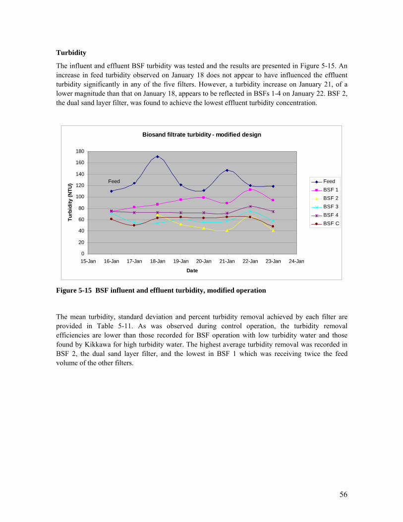
56

Turbidity

The influent and effluent BSF turbidity was tested and the results are presented in Figure 5-15. An increase in feed turbidity observed on January 18 does not appear to have influenced the effluent turbidity significantly in any of the five filters. However, a turbidity increase on January 21, of a lower magnitude than that on January 18, appears to be reflected in BSFs 1-4 on January 22. BSF 2, the dual sand layer filter, was found to achieve the lowest effluent turbidity concentration.

Biosand filtrate turbidity - modified design

0

20

40

60

80

100

120

140

160

180

15-Jan 16-Jan 17-Jan 18-Jan 19-Jan 20-Jan 21-Jan 22-Jan 23-Jan 24-Jan

Date

Turb

idity

(NTU

) FeedBSF 1BSF 2BSF 3BSF 4BSF C

Feed

Figure 5-15 BSF influent and effluent turbidity, modified operation

The mean turbidity, standard deviation and percent turbidity removal achieved by each filter are provided in Table 5-11. As was observed during control operation, the turbidity removal efficiencies are lower than those recorded for BSF operation with low turbidity water and those found by Kikkawa for high turbidity water. The highest average turbidity removal was recorded in BSF 2, the dual sand layer filter, and the lowest in BSF 1 which was receiving twice the feed volume of the other filters.

57

Table 5-11 BSF turbidity removal, modified design tests

Biosand filter Mean Turbidity (NTU)

Standard deviation (NTU)

Average turbidity removal

Feed 128 21

BSF 1 92 11 28%

BSF 2 52 12 59%

BSF 3 61 8 53%

BSF 4 74 4 42%

BSF C 60 7 53%

Table 5-12 compares the turbidity removal efficiency of each filter with its performance during the control testing stage of the field tests. The greatest increase in turbidity removal was seen in BSF 2, with a 38% increase over its control operation. This filter also produced the lowest filtrate turbidity of all the filters, possibly due to the extra depth of sand the water passed through. A significant 16% increase in turbidity reduction capacity was also observed in BSF 3, the very fine sand layer filter. BSF 1 operating under twice the feed volume of the other filters showed a 4% decrease in average turbidity removal; this is most likely attributable to general performance fluctuations as the effluent turbidity standard deviation was 11 NTU, compared to the mean value of 92 NTU. BSF 4 showed a 9% decrease in turbidity reduction, possibly a reflection of general performance variations. However, as the standard deviation of the filtrate turbidity was only 4 NTU, it may be likely that the filter performance has degraded, possibly due to clogging. The 4% increase in turbidity removal in BSF C is probably due to fluctuations in performance given the 7 NTU standard deviation of the filtrate turbidity.

Table 5-12 Change in filtrate turbidity after filter modifications

Biosand filter Change in turbidity removal

BSF 1 -4%

BSF 2 +38%

BSF 3 +16%

BSF 4 -9%

BSF C +4%

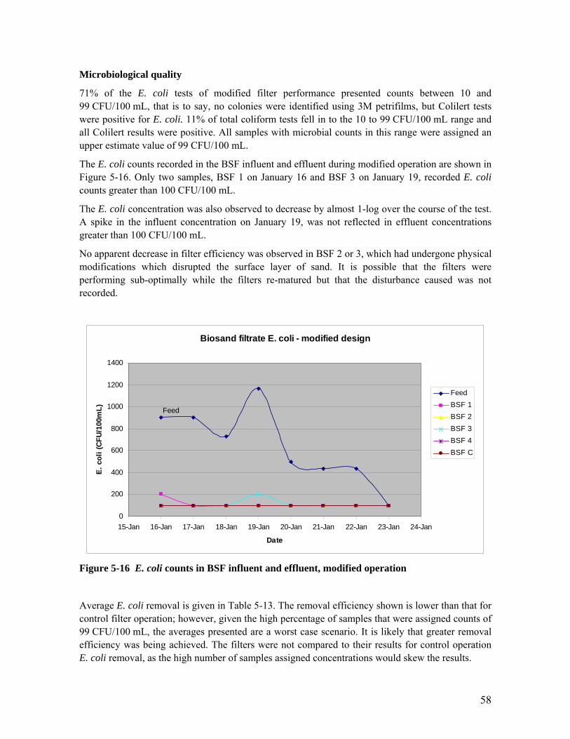
58

Microbiological quality

71% of the E. coli tests of modified filter performance presented counts between 10 and 99 CFU/100 mL, that is to say, no colonies were identified using 3M petrifilms, but Colilert tests were positive for E. coli. 11% of total coliform tests fell in to the 10 to 99 CFU/100 mL range and all Colilert results were positive. All samples with microbial counts in this range were assigned an upper estimate value of 99 CFU/100 mL.

The E. coli counts recorded in the BSF influent and effluent during modified operation are shown in Figure 5-16. Only two samples, BSF 1 on January 16 and BSF 3 on January 19, recorded E. coli counts greater than 100 CFU/100 mL.

The E. coli concentration was also observed to decrease by almost 1-log over the course of the test. A spike in the influent concentration on January 19, was not reflected in effluent concentrations greater than 100 CFU/100 mL.

No apparent decrease in filter efficiency was observed in BSF 2 or 3, which had undergone physical modifications which disrupted the surface layer of sand. It is possible that the filters were performing sub-optimally while the filters re-matured but that the disturbance caused was not recorded.

Biosand filtrate E. coli - modified design

0

200

400

600

800

1000

1200

1400

15-Jan 16-Jan 17-Jan 18-Jan 19-Jan 20-Jan 21-Jan 22-Jan 23-Jan 24-Jan

Date

E. c

oli (

CFU/

100m

L)

FeedBSF 1BSF 2BSF 3BSF 4BSF C

Feed

Figure 5-16 E. coli counts in BSF influent and effluent, modified operation

Average E. coli removal is given in Table 5-13. The removal efficiency shown is lower than that for control filter operation; however, given the high percentage of samples that were assigned counts of 99 CFU/100 mL, the averages presented are a worst case scenario. It is likely that greater removal efficiency was being achieved. The filters were not compared to their results for control operation E. coli removal, as the high number of samples assigned concentrations would skew the results.

59

Table 5-13 Average BSF E. coli removal, modified design tests

Biosand filter Mean E. coli (CFU/100 mL)

Standard Deviation (CFU/100mL)

Average E. coli removal

Feed 650 340

BSF 1 110 36 83%

BSF 2 100 0 85%

BSF 3 110 36 83%

BSF 4 100 0 85%

BSF C 100 0 85%

As a comparison, the removal efficiencies of samples assigned the maximum removal efficiency of 10 CFU/100 mL instead of 99 CFU/100 mL are shown in Error! Not a valid bookmark self-reference..

Table 5-14 BSF E. coli minimum and maximum removal efficiency, modified design tests

Biosand filter Maximum Average E. coli removal

Minimum Average E. coli removal

BSF 1 91% 83%

BSF 2 96% 85%

BSF 3 88% 83%

BSF 4 95% 85%

BSF C 98% 85%

Total coliform counts in the influent and effluent are provided in Figure 5-17. Large fluctuations were seen in the feed total coliform concentrations, but not in the E. coli profile. It is not known why the feed E. coli count showed a decreasing count trend, while the total coliform count showed an increasing trend, especially as good trend agreement be the two parameters was observed in the feed during the control tests. BSFs 2 and 3 which underwent physical modifications show elevated counts initially after the filters were brought back online, almost certainly due to disturbances to the biologically active layers.

60

The total coliform reading in BSF 2 on January 18 was considered to be an outlier caused by filtrate contamination during the modification process, due to its value being significantly higher than values on all other dates, this value has not been included in the filter performance calculations.

Biosand filtrate total coliform - modified operation

0

500

1000

1500

2000

2500

3000

3500

4000

4500

15-Jan 16-Jan 17-Jan 18-Jan 19-Jan 20-Jan 21-Jan 22-Jan 23-Jan 24-Jan

Date

Tota

l col

iform

(CFU

/100

mL)

FeedBSF 1BSF 2BSF 3BSF 4BSF C

Feed

Figure 5-17 Total coliform counts in BSF influent and effluent, modified operation

The total coliform removal efficiency of the BSFs is given in Table 5-15. All BSFs except number 3 achieved greater than 1-log average reduction of total coliforms. BSF 2 had the lowest standard deviation of the filters and the highest removal efficiency. While BSF 3 had the lowest removal and the highest standard deviation, it is likely that the filter was not performing at its full capacity due to disturbance of the schmutzdecke and biolayers during filter modification procedures.

61

Table 5-15 Average BSF total coliform removal, modified design tests

Biosand filter Mean total coliform (CFU/100 mL)

Standard Deviation (CFU/100mL)

Average total coliform removal

Feed 2870 728

BSF 1 250 151 91%

BSF 2 140 55 95%

BSF 3 430 410 85%

BSF 4 250 169 91%

BSF C 140 75 95%

As a comparison of maximum filter performance, the samples assigned 99 CFU/100 mL total coliform counts were reassigned 10 CFU/100 mL counts and the upper limit average removal efficiencies compared to the minimum efficiency achieved in Table 5-16. There is minimal difference between the minimum achieved and the theoretical upper limit average removal efficiencies.

Table 5-16 BSF total coliform minimum and maximum removal efficiency, modified design tests

Biosand filter Maximum Average total coliform removal

Average total coliform removal

BSF 1 92% 91%

BSF 2 96% 95%

BSF 3 85% 85%

BSF 4 94% 91%

BSF C 96% 95%

The change in total coliform removal of each filter compared to its efficiency during control operation is given in Table 5-17. The greatest difference in performance, with 7% change, was seen in BSF 3, which had undergone physical modifications. All other filters recorded change in removal efficiency of 4% or less, which is probably due to fluctuations in filter performance rather then improved or degraded performance. As 11% of the results were assigned 99 CFU/100 mL total

62

coliform counts, the change in performance represents the minimum average filter efficiency that could have occurred.

Table 5-17 Change in filtrate total coliform removal after filter modifications

Biosand filter Change in total coliform removal

BSF 1 +2%

BSF 2 +4%

BSF 3 -7%

BSF 4 -3%

BSF C +4%

5.4 Recommendations Testing of the modified BSF designs was conducted over a period of eight days. Testing should be conducted to compare filter field performance over a longer duration of operation to firstly, ensure that the modified filters had ripened, and secondly, to provide a larger data set from which to draw filter efficiency comparisons.

As many of the microbiological test results fell in the 10 to 99 CFU/100 mL range, using the 3M Petrifilm and Colilert testing technologies, supplemental testing methods should be used, such as membrane filtration, to allow for detailed enumeration of total coliform and E. coli concentrations.

From the results available, the modified dual sand layer BSF (BSF 2) performed better than the control BSFs and the superfine sand layer BSF (BSF 3) for both turbidity and total coliform removal efficiency. Due to the method of testing microbiological water quality (3M Petrifilm and Colilert assays) the filter performances for E. coli reduction efficiency were inconclusive.

Considering that turbidity is an indirect measure of microbial count (Reynolds and Richards, 1996) the increased turbidity reduction achieved by BSFs 2 and 3 suggests that increased E. coli removal could have occurred and further testing of these systems should be conducted.

One drawback of the dual sand layer BSF (BSF 2) was the low flow rate resulting from the decreased filter freeboard available to support the pressure head required for higher flow rates. This is an important design factor; however, it is a parameter that can be optimised through modifications to the filter layout, for example by increasing the freeboard.

The field testing of the dual sand layer BSF (BSF 2) showed promising turbidity and microbiological removal efficiencies and this filter was selected for further study and design optimisation in the MIT laboratory.

63

6. Dual sand layer biosand filter design optimisation The dual sand layer biosand filter design studied in Tamale (as Tamale BSF 2) and shown in Figure 6-1 was selected for further study and design optimisation in the MIT Civil and Environmental Engineering laboratory during the period February to May 2009.

Figure 6-1 Field test dual sand layer biosand filter

As with the field tests conducted in Tamale, Ghana, the laboratory optimisation tests of two filters were carried out in two phases:

a. Two unmodified single sand layer filters were operated as control filters to give baseline performance data. This enabled comparison of the different filters prior to modification and comparison of the modified filters to pre–modification performance.

b. Testing of one dual sand layer filter and one control filter simultaneously. Dual sand layer filter performance was evaluated against its baseline performance in phase a. and against the control filter in phase b.

6.1 Dual sand layer BSF design Three aspects were considered essential to the optimisation of the dual sand layer biosand filter (DSL BSF) for treatment of highly turbid water, and were addressed during this stage of the study:

• Filter cleaning program for high turbidity source water

• Supporting biological activity for oxidation filtration in the lower sand layer

• Design of the upper sand layer

6.1.1 Filter cleaning Management of the sediment load in high turbidity water is necessary to ensure smooth BSF operation. There are two common ways to manage the sediments: removal/reduction of sediments prior to pouring the water into the BSF, or, frequent BSF cleaning to remove sediment build-up on the top of the sand.

Upper sand layer

Lower sand layer

64

In their training sessions for BSF use in areas with highly turbid water, CAWST recommends the use of particle removal processes to reduce the particulate load entering the filter, thereby reducing the frequency of filter cleaning and subsequent disturbance of the biologically active layers. Particle removal processes recommended by CAWST for the Tamale area include coagulation/flocculation and sedimentation technologies such as alum or Moringa dosing. CAWST suggests cleaning the filter using the “swirl and dump” method only when the filter flow rate becomes too slow. (CAWST, 2009a) However, using an additional particle removal process which involves the ongoing purchase of coagulant, i.e. alum or Moringa, was eliminated as an option in section 5.1.1 as it is likely to be cost prohibitive to many poor people in developing regions.

Alternatively, frequent filter cleaning is required, which occurs in four villages in northern Ghana: Gbabshie, Zuozugu and Kpanvo, all in the Tamale area, and Batamyili, in Savelugu, where blanket distribution of International Aid HydrAid™ BSFs had been carried out during the previous year. These villages were visited in January 2009 as part of the research for this thesis, and informal conversations with filter operators disclosed that they had been instructed to clean their filters, using the “swirl and dump” technique, every three days.

With such a rigorous cleaning program required to maintain filter flow, the schmutzdecke would have been highly disturbed. Based on information in the BSF manual produced by CAWST (2008) which states that biological layers can take up to a week to re-establish after cleaning, it is probable that the schmutzdecke and upper biolayers in these filters would not have had sufficient time to re-mature before the next cleaning session occurred. The consequence of this is sub-optimal oxidation filtration of the feed water and higher risk of pathogenic contamination remaining in the drinking water.

As the inclusion of a coagulation-flocculation step was considered to be too expensive and complex, filter cleaning was focused on as the mechanism to manage the particulate load in the filter.

To accommodate the necessity of regular filter cleaning, the DSL BSF was designed to support predominantly mechanical filtration in the upper sand layer, with oxidation filtration mostly occurring in the biologically active layers developed in the lower sand layer.

Should the DSL BSF flow rate slow due to clogging of the lower sand layer, the upper sand layer is designed to be lifted out of the BSF to allow “swirl and dump” cleaning of the lower sand layer. As with a single sand layer BSF, this will disturb the biolayers which will also need sufficient time to re-mature before the filter is operating at full efficiency. If possible, water poured in the filter during the re-maturation period should be treated after filtration to mitigate higher microbial concentrations that may be present in the filtrate.

6.1.2 Biological filtration process As biosand filtration is an aerobic oxidation process, maintaining oxygen flow to the biologically active layers in the first sand layer during the pause phase of operation was a critical design element of the DSL BSF.

The capacity of water to hold dissolved oxygen is a function of water temperature, such that, as the temperature increases, saturation concentration of dissolved oxygen in the water decreases. Dissolved oxygen saturation concentrations in water as a function of temperature are provided in Appendix E.

65

Dissolved oxygen supply in single sand layer BSFs

In single sand layer BSFs, sufficient dissolved oxygen quantities reach the biologically active layers to support the biological metabolism of organic contaminants through diffusion of oxygen across the supernatant. Buzunis (1995) described oxygen diffusion across the supernatant using the thin film model, for mass transfer across an air-water interface. This model assumes that a dissolved chemical has a uniform concentration throughout the air and water as a result of turbulent diffusion, except for thin films, each of air and water, at the interface where turbulent diffusion is suppressed (Hemond and Fechner-Levy, 2000). The thin air and water films increase resistance to chemical mass transfer between the air and water and are considered to be rate-limiting to chemical diffusion (i.e. mass transfer) at the air-water interface as only molecular diffusion occurs (Hemond and Fechner-Levy, 2000). Buzunis determined that resistance to oxygen diffusion in the air film is negligible due to the low solubility of oxygen; subsequently, the oxygen diffusion is controlled by the water side of the air-water boundary. Figure 6-2 shows the water-side controlled oxygen diffusion pathway in a single sand layer BSF.

Figure 6-2 Oxygen diffusion pathway in a single sand layer BSF The mass flux of oxygen across the supernatant was expressed by Buzunis as the sum of mass flux across the thin water film, described by the thin film model (Equation 1), and one dimensional mass flux across the supernatant water body, described using Fick’s Law of diffusion (Equation 2):

)( bsat CCKJ −= Equation 1

zCC

DJ bsandm

−−= Equation 2

where: J is the mass flux of oxygen (mg/(m2s)) K is the gas exchange coefficient involving the temperature and resistance to mass transfer between phases (m/s) Csat is the saturation concentration of dissolved oxygen in water at a given temperature (mg/m3)

Air – turbulent diffusion

Thin water film – molecular diffusion

Supernatant – turbulent diffusion

Oxygen dissolved in water

Oxygen in air

Fine sand layer – turbulent diffusion

66

Cb is the concentration of dissolved oxygen in the thin water film just inside the air- water interface (mg/m3) Csand is the concentration of dissolved oxygen just above the fine sand layer (mg/m3) Dm is the molecular diffusivity of oxygen in water (m2/s) z is the total depth of the supernatant (m; thin film plus supernatant).

Buzunis expressed the total mass flux across the whole of the supernatant by combining Equations 1 and 2, as shown in Equation 3:

)( sandsatm

m CCDKzKD

J −+

−= Equation 3

To maintain aerobic conditions in the filter, Buzunis recommended that the minimum allowable concentration of dissolved oxygen in the biolayers be 1 mg/L. Based on this, using Equation 3, and a water temperature of 20°C, Buzunis established an optimal supernatant depth of 5 cm.

Dissolved oxygen supply in dual sand layer BSF

With a dual sand layer system the diffusion rate from the air through the supernatant to the lower sand layer is slowed by the presence of the upper sand layer, as illustrated in Figure 6-3. The lower rate is a result of mass transfer only occurring in the pore spaces between the sand particles.

Figure 6-3 Oxygen diffusion pathway in a dual sand layer BSF

Oxygen in air

Oxygen dissolved in water

Air – turbulent diffusion

Thin water film – molecular diffusion

Supernatant – turbulent diffusion

Fine sand layer – turbulent diffusion Lower sand layer

Fine sand – turbulent diffusion

Coarse sand – turbulent diffusion

Water layer – turbulent diffusion

Upper sand layer

67

Dissolved oxygen will diffuse through the thin water film and supernatant with the same flux mechanism as the single sand layer BSF, and can be calculated using Equation 3.

As the dissolved oxygen reaches the upper sand layer, the oxygen diffusivity will be affected by the porosity of the sand. Archie’s Law (Archie, 1942 from Chen, 1993) correlates chemical diffusivity in water with chemical diffusivity through water saturated sediments as shown in Equations 4 and 5:

)(' nnDD mm = Equation 4

with, 1−= mnn Equation 5

where Dm is aqueous solution diffusivity (m2/s) Dm’ is diffusivity in sediments (m2/s) n is the porosity (dimensionless) m is a factor related to porosity.

Ullman and Aller (1982) suggest that m = 3 for n ≥ 0.7 and m = 2 for n < 0.7 (from Chen, 1993).

The fine sand used in the DSL BSF construction was <1 mm in diameter, with fine particles removed during the washing process. Measurement of the fine sand porosity in the MIT laboratory, by filling a 1 L plastic beaker with sand and filling pore space with water (390 mL) until one litre of sand plus water was contained in the beaker, indicated the fine sand porosity was 0.39, which was rounded to 0.4. This measured porosity is inline with the US EPA (1998) literature stating that the porosity range for sand of this size is 0.31 to 0.46; Buzunis (1995) also used 0.4 for his calculations. For the BSF coarse sand layer, 3-6 mm diameter, the US EPA (1998) indicates a porosity range of 0.25 to 0.38, and for this study a value of 0.3 was used.

Based on the fine sand and coarse sand porosities, an m-value of 2 was used in Equation 5. From these values, the dissolved oxygen flux through the upper sand layer is limited by the flux through the coarse sand layer due to the lower porosity.

With the diffusivity corrected for flow through sediments, the flux of oxygen through the upper sand layer, of depth z and porosity corresponding to coarse sand, can be approximated with Equation 6:

zCC

nDJ arsesandbottomofcoesandtopofcoarsm

−−= ' Equation 6

Oxygen will then diffuse through the water between the upper and lower sand layers at a rate controlled by the flux through the upper sand layer (i.e. the rate limiting flux) and can be modelled using Fick’s Law of diffusion (Equation 7).

zCC

DJ barsesandbottomofcom

−−= Equation 7

However, any microbial activity in the upper sand layer will cause some, or all, of the oxygen diffusing from the air to be consumed, further limiting the concentration of dissolved oxygen reaching the first sand layer. The consumption rate of the dissolved oxygen, also called the biochemical oxygen demand (BOD), is dependent on the microbial species and concentrations present in the source water and is therefore a local condition. Furthermore, the microbial

68

consumption rate of oxygen is a function of temperature, such that for every 10°C increase in water temperature the oxygen consumption rate doubles (Buzunis, 1995). Therefore, a key factor in the design of the DSL BSF was to minimise oxygen consumption in the upper sand layer in order to achieve the highest concentration of oxygen reaching the upper sand layer.

In addition to minimising oxygen consumption in the upper sand layer, the depth of water layers and the upper sand layer in the DSL BSF were designed to allow sufficient oxygen concentrations to diffuse through to the lower sand layer to support the aerobic oxidation filtration process.

6.1.3 Raised upper sand layer design

Upper sand layer depth

The role of the upper sand layer is to provide an additional mechanical filtration stage to the filter. It was expected biological activity would attempt to colonise the upper sand layer, however, this should be controlled by the 3-day cleaning program, which would disturb any biological activity present in the upper sand layer and the associated biochemical oxygen demand will be minimised. To maintain oxygen flux to the lower sand layer, keeping the depth of the upper sand layer to a minimum was important in the design.

Upper sand layer location

The freeboard height controls the volume of water that can be poured into the filter above the supernatant. With greater water depth, increased pressure head drives the water through the filter at a faster flow rate. The fast flow rate of the single sand layer BSF is a design feature that many users like, so maintaining this was an important design consideration. Freeboard depth can be controlled by the location of the upper sand layer. To sustain a suitable freeboard, the depth of the lower sand layer was adjusted.

As with the single sand layer BSF, the depth of the supernatant controls the oxygen diffusion flux to the uppermost sand layer. With the raised upper sand layer hindering the oxygen flow to the lower sand layer, one focus of the DSL BSF design was to maximise the oxygen concentration reaching the biologically active sand in the lower sand layer by adjusting the depth of the supernatant. CAWST (2008) suggest that in some climates where high evaporation rates are experienced, the supernatant can evaporate down to the sand, destroying the biolayers. They recommend a minimum supernatant depth of 5 cm to prevent this. Significant evaporation of the supernatant was not witnessed in the Tamale field tests, which were conducted in a hot, dry region. In addition, as the upper sand layer was not designed to achieve biological filtration, the depth of the supernatant is not considered as critical for the DSL BSF as it is for a single sand layer BSF. It is not desirable for the supernatant to evaporate down to the upper sand layer but should this occur, the mechanical filtration efficiency of the upper sand layer should not be grossly affected, nor the biological activity in the lower sand layer.

The depth of the upper sand layer controls the oxygen diffusion flux to the biologically active lower sand layer. Ideally the upper sand layer should be kept as shallow as possible to maximise oxygen flux while effectively providing mechanical filtration to the water.

Finally, the depth of the water between the upper and lower sand layers further controls the concentration of dissolved oxygen reaching the biologically active lower sand layer. It was desirable to find a balance between providing minimal depth for oxygen to diffuse through and

69

sufficient depth for turbulent mixing of the dissolved oxygen entering from the upper sand layer. Turbulent mixing of the dissolved oxygen in this water layer is essential in the planar direction, to provide more even distribution of the oxygen received from the upper sand layer and vertically, to move the oxygen received down to the first sand layer and replace that removed by oxidation at a rate faster than molecular diffusion would provide.

Table 6-1 provides a summary of the essential considerations in the design of the laboratory operation DSL BSF and the purpose of each consideration.

Table 6-1 DSL BSF upper sand layer design parameters

Design Parameter Purpose

3-day cleaning program Control upper sand layer BOD Control filter clogging, therefore flow rate

Freeboard height Control filter flow rate

Supernatant depth Facilitate oxygen diffusion

Upper sand layer depth Control upper sand layer BOD Facilitate oxygen diffusion

Water depth between upper and lower sand layers

Facilitate biological activity in lower sand layer Facilitate turbulent diffusion of oxygen

6.2 Dual sand layer BSF set up and operation

6.2.1 Filter set up During December 2008, two plastic BSFs were set-up in the MIT laboratory using Kanchan™ Arsenic BSF plastic filter shells, pipe work and diffuser basins from Nepal. Both the Kanchan™ Arsenic filter and the filters used in the Tamale field tests have a 50 L capacity.

Following the set up procedure by Ngai et al. (2006a), 10 L of tap water (Cambridge Water Department reticulated supply) were added to the empty filters. 6 L of 6-15 mm washed gravel was then placed in each filter, followed by 4 L of 3-6 mm washed coarse sand. The instructions then specified placement of 20 L <1 mm fine sand, however, the outlet pipe work limited the volume of sand that could be added in order to maintain the supernatant 5 cm deep, and due to the limited availability of fine sand at the time, 16 L was added to one filter and 15 L to the other. Hereafter the BSF with 16 L fine sand is referred to as BSF A and the BSF with 15 L fine sand as BSF B. The supernatant depth was 6 cm in BSF A and 7.5 cm in BSF B.

The filters were flushed with 15 L of water collected from the Charles River, adjacent to the MIT laboratory. The filters were not operated during the remainder of December 2008 or January and February 2009.

70

6.2.2 Test procedures As with the field tests, all laboratory optimisation tests were conducted in a manner that reduced possible contamination of samples from external sources. All BSFs were sampled for turbidity and microbiological quality after approximately 5 L of filtrate had been discharged, so that diurnal results were comparable.

Flow rate

Maximum flow rates (in litres per minute) were measured immediately after the filters had been filled by holding laboratory type 1 L plastic beaker under the outlet for 30 seconds and measuring the volume.

Turbidity

Turbidity measurements were conducted with a Hach 2100P Turbidimeter as outlined in Section 5.3.1. Turbidimeter calibration was checked approximately every three days, and recalibrated if the reading was greater than 2 NTU from the formazin standard.

Microbiological Quality

All of the microbiological testing was carried out in a sterile environment in the laboratory at the MIT Civil and Environmental Engineering Department (CEE) Laboratories. All surfaces were wiped down with isopropyl alcohol before each test commenced and either sterile disposable equipment was used or testing equipment was sterilised in boiling water.

To replicate field conditions, water samples were collected in sterile 100 mL Whirl-Pak® Thio-Bags®. All samples were immediately tested.

Initially testing was conducted using 3M Petrifilm E. coli / Coliform Count Plates and IDEXX Colilert presence/absence tests. Towards the end of test 1, the E. coli and total coliform counts fell into the 10-99 CFU/100 mL range, that is, no counts shown on the 3M Petrifilms and positive Colilert results. To better understand the degree of microbiological reductions membrane filtration (MF) was commenced in addition to the 3M Petrifilm and Colilert tests.

MF tests were conducted in accordance with Millipore guidelines, which are adapted from the U.S. Standard Methods for the Examination of Water and Wastewater (20th Edition, 1998). Samples were cultured using m-ColiBlue24® Broth Coliform and E. coli Detection Media for use with Membrane Filter Technique marketed by the Hach Company, USA. A Millipore Portable Membrane Filter XX6300120, Robens (Surrey, United Kingdom) recyclable petri dishes, Millipore all metal syringe XX6200035, Pall Corporation GN-6 grid 47 mm 0.45 μm filters and Pall Corporation pads for 47 mm filters were used.

The 3M Petrifilm, Colilert and MF petri dishes were incubated in the MIT CEE laboratory at 35°C for 24±2 hours using a Millipore XX6310000 Incubator.

8% of 3M Petrifilm tests, 12% of Colilert tests and 6% of MF tests were duplicated for accuracy monitoring of results. One blank sample for every 14 3M Petrifilm, every 13 Colilert test, and every 32 MF tests was analysed for accuracy monitoring of the test methods. The duplication of and running blank tests for the MF method was limited by the quantity of m-ColiBlue24® Broth available.

71

In cases where less than 100 CFU/100 mL were registered using the 3M Petrifilm, the Colilert test registered positive for more than 10 CFU/100 mL and MF testing was not undertaken, a value of 99 CFU/100 mL was assigned to the sample as the upper contamination limit. Where the Colilert test registered negative for more than 10 CFU/100 mL and MF testing was not carried out, a value of 9 CFU/100 mL was assigned as the upper contaminant limit. Final results are also compared using a lower threshold value of 10 CFU/100 mL for results that fell into the 10 – 99 CFU/100 mL range and using 0 CFU/100 mL for results that were negative for both 3M Petrifilm and Colilert tests, to show the theoretical maximum performance for the results achieved.

Dissolved oxygen concentration

Dissolved oxygen concentrations were measured using a YSI Model 57 Oxygen Meter with YSI Model 5239 probe. Prior to testing each day the precision of the probe membrane was confirmed by measuring the concentration of dissolved oxygen saturated water and compared to the theoretical value for water at the same temperature. Dissolved oxygen saturation concentrations in water as a function of temperature are provided in Appendix E. Cambridge Water Department potable reticulated water which had been allowed to sit in the laboratory for a minimum of 24 hours to become saturated was used for the saturation test. To accurately measure the dissolved oxygen concentration the probe was swirled in the water to create flow past the probe membrane (Frankel, 2009).

Dissolved oxygen readings were taken in situ for the supernatant of BSFs A and B and for the water layer between the upper and lower sand layers for BSF B (through the ports illustrated in Figure 6-6). Recordings were taken immediately above the sand surface for consistency and to gauge the oxygen concentration reaching the sand. Minimal swirling of the probe was required for the readings and was undertaken in a manner to cause least disturbance to the sand and schmutzdecke. The BSF effluent was captured in a polyethylene bag for immediate reading. Contact between the air and the effluent was kept to a minimum to protect the integrity of the sample.

6.2.3 Reproduction of dugout water In order to compare laboratory filter performance with the Tamale field tests, water with similar turbidity and microbial quality to that found in Tamale dugouts was required. Water from the Charles River was used as a base, as the Cambridge Water Department potable reticulated supply contained chlorine residual that would interfere with the formation of biological layers in the BSF. The typical water quality of the Charles River during the study period is presented in Table 6-2.

Table 6-2 Charles River water quality

Parameter Charles River, March 2009 Charles River, April 2009

Temperature (°C) 4 14

Average turbidity (NTU) 6 5

E. coli (CFU/100 mL) 10-99 10-99

Total coliform (CFU/100 mL) 10-99 10-99

72

Temperature

The laboratory study was conducted at the end of the northern hemisphere winter, and at the commencement of this work the Charles River was partially frozen over. To counter any influence on the test results caused by such low temperatures, water was collected 24 hours before intended use and placed in the laboratory which had an average ambient temperature of 27°C. The average water temperature at the time of use was 23°C.

Turbidity

To mimic the turbidity of Tamale dugout water, clay was added to the Charles River feed water. The target turbidity was in the range of 100 – 200 NTU, similar to the turbidity range in Fuo Mwale dugout (refer to Table 5-2). Some fluctuations in the laboratory water turbidity were desired, replicating the dugout turbidity results.

Powdered white clay purchased at a ceramic art supply store was added to the water. Over a five day period, the Charles River water was spiked to a turbidity ranging from 112-158 NTU, and 10 L/day of turbid water was added to each filter imitating the same operating procedure followed for the filters used in the field tests in Tamale, Ghana. The filtrate of both BSFs was measured in the range 1 – 3 NTU, significantly better turbidity removal than the BSFs tested in the field. It was noted that buckets of Charles River water spiked with clay and left to settle for 24 hours experienced approximately 90% reduction in turbidity at the water surface. The ambient surface turbidity level after a 24 hour settling period averaged 26 NTU. During filter filling cycles, it was observed that the turbidity of the feed water in the diffuser plate reduced from 158 NTU to 53 NTU in BSF A and 59 NTU in BSF B over a 30 minute period. Due to the rapid settling of the white clay, the turbidity removal efficiency of the BSF was not able to be accurately studied with this turbidity source.

As the focus of the tests was to reproduce the conditions in Tamale, an alternative source of turbidity which would not be filtered from the water with such high efficiency was sought. A powdered red clay also purchased at a ceramic art supply store, dried dugout clay brought back from Tamale by a student in January 2008 and locally sourced wet Boston blue clay were all used to spike the Charles River water within the range 100-200 NTU. However, as with the white clay, these three clays were also filtered with the same high degree of efficiency from the feed water.

It is uncertain why such efficient turbidity removal occurred in the MIT laboratory BSFs as opposed to the Ghana field study and it was initially thought to be a result of clay particle size, such that the laboratory clay particles were larger and settling from the water faster. To test this theory, a bucket of white clay spiked water, with initial turbidity >2,000 NTU was allowed to settle for one week. At the end of the week the turbidity of water decanted from the top of the bucket was tested to be >100 NTU, in theory only fine clay particles should have remained in this suspension. The feed water was then spiked with this clay suspension, however, BSF turbidity removal efficiency did not decrease. It was assumed that the efficiency of the filters to remove clay turbidity was not a function of clay particle size but another cause. The cause of the high clay turbidity removal rate remained unknown although it was speculated to be a result of compatible electrostatic forces between the sand media and/or biofilm and the clay particles.

73

All Charles River water fed to the BSFs for the remainder of the study was spiked with the locally sourced Boston blue clay due to its ease of use. There was an insufficient quantity of the Tamale sourced dugout clay to complete the research so this was not used.

Microbial quality

To recreate the water quality of the Tamale dugouts measured in January 2009, the E. coli and total coliform counts in the water were augmented with raw screened sewage from the South Essex Sewage District Wastewater Treatment Plant in Salem, Massachusetts which had been tested for E. coli and total coliform counts. Measured quantities of sewage were then added to the Charles River source water to imitate the mean microbial counts found in the Fuo Mwale dugout, 1,200 CFU/100 mL E. coli and 4,000 CFU/100 mL total coliform.

The sewage was stored in a refrigerator at 8°C. It was noticed that the microbial counts in the sewage decreased over time and the quantity of sewage added to the feed water was increased accordingly.

6.2.4 Control filter operation efficiency During March 2009, the two filters were operated simultaneously as single sand layer control BSFs using Charles River water at room temperature. The water was spiked with clay for turbidity to compare filter performance in terms of turbidity removal efficiency. The average temperature of the clay-spiked feed water was 24°C and each filter was filled with 10 L of spiked water per filling session. Table 6-3 provides a summary of the flow rate and turbidity removal performance of the two filters. E. coli and total coliform quality was not tested.

Table 6-3 BSF flow rate and turbidity removal during control tests

Parameter Average flow rate (L/min)

Average turbidity (NTU) (Standard deviation)

Feed water 153 (41)

BSF A 0.4 6 (4)

BSF B 0.7 6 (4)

The comparison of the two filters during the control showed that both filters achieved the same turbidity removal efficiency, 97%, but that BSF B operated at a flow rate 166% higher than BSF A. The difference in flow rates is most likely a result of sand grain arrangement, formation of the schmutzdecke and biofilm on the sand and/or possible short-circuiting in the filter. While the microbiological removal efficiency of the filters was not monitored, ripening of the biologically active zone would have occurred to some extent.

74

6.2.5 Filter modifications After testing the single sand layer performance of the filters, modifications to each filter were made, as follows:

BSF A – single sand layer biosand filter

In BSF A the volume of fine sand was increased to 18 L, short of the 20 L recommended in the Kanchan™ Arsenic Filter construction manual (Ngai et al., 2006a), but the maximum volume of sand that could be added whilst maintaining the supernatant layer. It was intended the supernatant layer would be 5 cm deep, however, final measurements indicated it was closer to 3.4 cm. A diagram of BSF A is provided in Figure 6-4.

Figure 6-4 Single sand layer biosand filter (BSF A)

BSF B – dual sand layer biosand filter

BSF B was modified to operate as a dual sand layer BSF, as shown in Figure 6-5. The filter system was designed to fit within the standard 50 L Kanchan™ Arsenic Filter while maintaining sufficient freeboard for a fast flow rate. To do this, the lower sand layer depth created by using only 15 L fine sand (<1 mm) was maintained. A 2 cm layer of water was created between the lower sand layer and the upper sand layer to facilitate turbulent mixing of dissolved oxygen.

It was intended that the upper sand layer would be supported by a diffuser plate, constructed from a plastic basin deeper than that used in a single sand layer BSF and commonly available in Tamale, Ghana, and other developing regions. However, plastic basins of this size could not be easily sourced in the USA, and the base of a plastic pot plant holder, referred to as the support plate

Diffuser Plate 14cm deep

41cm

Lid

Outlet

Underdrain 33cm

Single sand layer 18 L Fine Sand (<1 mm) 19.6 cm

6 L Gravel (6-15 mm) 5 cm 4 L Coarse Sand (6-15 mm) 3.5 cm

Supernatant 3.4 cm

Freeboard 15.5 cm

Schmutzdecke

75

hereafter, was modified and used instead. Because the support plate did not have a rim that could hang from the shell of the BSF, as the diffuser plate does in the single sand layer LPD BSF, it was supported on the lower sand layer using sterile plastic centrifuge vials sourced from the laboratory. The space between the edge of the support plate and the BSF shell was sealed off using three layers of Parafilm® M to prevent feed water bypassing the upper sand layer. Pebbles were placed on the Parafilm® M to hold it in position and the integrity of the seal was checked daily for the duration of the study and confirmed to have remained intact.

Water flowed through the bottom of the support plate via 20 2 mm holes drilled through the base. A 1 cm layer of coarse sand (3-6 mm) was placed on the base of the support plate to prevent the fine sand falling through the holes. A 2 cm layer of fine sand (<1 mm) was added on top of the coarse sand.

The resulting depth of the supernatant was 2.7 cm and it was decided to carry out the study tests at this depth as it provided less resistance to oxygen diffusion.

Figure 6-5 Dual sand layer biosand filter (BSF B)

Ports through the upper sand layer were installed to allow testing of the dissolved oxygen concentration in the water layer between the lower and upper sand layers, as shown in Figure 6-6.

Three ports were installed, one in the centre and two at the edges of the filter, with the intention of averaging the concentrations. VWR International 50 mL disposable centrifuge tubes with screw caps (catalogue number 21008-242) were used as ports and secured into the base of the support plate. These centrifuge tubes were selected as the diameter was only several millimetres greater than the dissolved oxygen probe (YSI Model 5239 probe) and therefore only minimal ingress of oxygen

Outlet

41 cm

33 cm

15 L Fine Sand (<1 mm) 15.3 cm

6 L Gravel (6-15 mm) 5 cm

4 L Coarse Sand (6-15 mm) 3.5 cm

Supernatant 2.7 cm

Freeboard 15.5 cm

Water layer 2 cm

Fine Sand (<1 mm) 2 cm Coarse Sand (3-6 mm) 1 cm

Lid

Diffuser Plate 14cm deep

Underdrain

Lower sand layer

Upper sand layer

Support plate

Parafilm® M seal

Schmutzdecke

76

into the port and therefore into the lower sand layer would occur during oxygen measurements. Gaps between the ports and the support plate were sealed with Parafilm® M to prevent localised dissolved oxygen sources influencing the test results. The port screw caps were tightly fitted at all times, except during testing, to prevent oxygen entering the water directly from the air.

Figure 6-6 BSF B set-up for dissolved oxygen concentration measurements

Figure 6-7 is a plan photo of the BSF B upper sand layer showing dissolved oxygen ports.

Figure 6-7 DSL BSF upper sand layer and dissolved oxygen measurement ports (Source: Collin, 2009)

Dissolved oxygen measurement port

Parafilm® M seal

Upper sand layer

Port for dissolved oxygen measurements

Lower sand layer

Support plate

Parafilm® M seal

77

6.3 BSF optimisation tests and results The filters were tested under three sets of operating conditions, detailed in Table 6-4.

Table 6-4 BSF optimisation tests

Test Filling cycles per day

Volume of fill (L) 3 day cleaning program

Duration of test

1 1 10 no 12 days

2 1 10 yes 8 days

3 2 10 or 20 yes 4 days

During test 1, the filters were compared for performance without disturbance to any of the sand layers from the cleaning program. The results were also monitored to ensure that filter ripening had occurred.

The aim of the second test was to monitor the effect on filter performance of the 3 day cleaning program and associated disruption to the schmutzdecke.

The third test investigated the effects on the filtered water quality firstly, due to the effect the length of the pause phase on the filtrate quality and secondly, when the fill volume exceeded the 10 L pore volume of the filter such that some water passed straight through the filter without being treated during the pause phase.

For the duration of the laboratory tests the source water (spiked Charles River water) and the BSF filtrate were monitored for turbidity and microbial quality with total coliform and E. coli as an indicator organism for faecal contamination.

6.3.1 Feed water quality The water for each test was sourced from the Charles River and spiked with Boston blue clay to increase turbidity and sewage sourced from the South Essex Sewage District in Salem, Massachusetts.

Table 6-5 is a summary of the feed water characteristics used in the optimisation study between March 11 and May 4, 2009, using sewage collected April 10. For the second test run on May 4 (test 3) until the end of the test period on May 6, 2009, sewage collected on May 4 was used and the feed microbiological concentrations increased significantly.

Table 6-6 shows the feed quality during this period.

78

Table 6-5 BSF Feed water characteristics, optimisation study, March 11 to May 4

Statistic Turbidity (NTU)

Total coliform (CFU/100 mL)

E. coli (CFU/100 mL)

Temperature (°C)

Minimum 116 200 99 20

Maximum 287 5,500 1,100 26

Mean 183 2,190 250 23

Median 173 1,460 200 23

Standard deviation 49 1,850 230 2.1

Table 6-6 BSF Feed water characteristics, optimisation study, May 4 to May 6

Statistic Turbidity (NTU)

Total coliform (CFU/100 mL)

E. coli (CFU/100 mL)

Temperature (°C)

Minimum 128 8,700 3,700 20

Maximum 183 9,500 4,800 23

Mean 148 9,100 4,330 21

Median 140 9,100 4,400 21

Standard deviation 24 3,700 520 1.4

6.3.2 Test 1 results In Test 1, the two BSFs were filled with 10 L water once each day. The filters were not cleaned using the “swirl and dump” method during this test.

Flow rate

Figure 6-8 shows that the flow rates for the two filters were essentially constant over the test period. Filter clogging was not observed even though the raw water turbidity was high.

79

Biosand filter flow rates - test 1

0

0.1

0.2

0.3

0.4

0.5

0.6

0.7

0.8

11-Apr 13-Apr 15-Apr 17-Apr 19-Apr 21-Apr 23-Apr 25-Apr

Date

Flow

rat

e (L

/min

)

BSF ABSF B

Figure 6-8 BSF flow rates, test 1

The average filter flow rates are provided in Table 6-7. As was noted during the control tests of the filters, the flow rate of BSF B was much higher than that of BSF A, which was attributed to possible influences from the sand grain arrangement, the formation of the schmutzdecke and biofilm on the sand and/or possible short-circuiting in the filter.

Table 6-7 BSF flow rates, test 1

Biosand filter Flow rate (L/min)

BSF A 0.4

BSF B 0.7

Turbidity

As discussed in Section 6.2.3, difficulty was encountered maintaining clay in the feed water in suspension. The performance of the laboratory filters did not correlate with that of the field filters. In this optimisation study, both BSF A and BSF B achieved an average turbidity reduction of 98%.

Microbiological Quality

During much of this test the E. coli and total coliform concentrations were only tested using 3M Petrifilm and Colilert methods. MF was used on the last two days of the test. 38% of BSF A and 46% of BSF B E. coli values fell into the range 10-99 CFU/100 mL and were assigned

80

99 CFU/100 mL values; 15% of BSF A and 23% of BSF B E. coli results were assigned concentrations 9 CFU/100 mL. 38% of both BSF A and BSF B were assigned total coliform values in the 10-99 CFU/100 mL range and 8% of BSF B total coliform values were assigned 9 CFU/100 mL.

Figure 6-9 compares the feed and filtrate E. coli concentrations of the two filters. As so many of the filtrate samples were assigned 99 or 9 CFU/100 mL values, it was difficult to compare the filter performance or establish removal efficiencies. The filters both fell into the <10 CFU/100 mL concentration range around the period April 19 to 21 suggesting comparable filter performance during this test. It was surmised that filter ripening also occurred during this time.

Biosand filtrate E. coli - test 1

-200

0

200

400

600

800

1000

1200

10-Apr 14-Apr 18-Apr 22-Apr

Date

E. c

oli (

CFU

/100

mL)

FeedBSF ABSF B

Feed

Figure 6-9 E. coli counts in BSF influent and effluent, test 1

Table 6-8 shows that BSF A achieved 75% E. coli reduction and BSF B a slightly higher 79% reduction. Based on the MF test results for the last two days, both BSFs reduced E. coli concentrations by an average of >99%, or, a 2-log reduction. It is also likely that a schmutzdecke layer was forming on the surface of the upper sand layer of BSF B during this time, as the sand was undisturbed, and although this was not the intention of the design it was unavoidable during this stage of testing.

81

Table 6-8 BSF E. coli removal efficiency, test 1

Biosand filter Mean E. coli (CFU/100 mL)

Standard Deviation (CFU/100mL)

Average E. coli removal

Feed 308 269

BSF A 78 58 75%

BSF B 64 47 79%

Results were also assessed for the theoretical maximum performance efficiency by assigning lower threshold values of 10 CFU/100 mL to the tests with indicator bacteria counts in the 10 – 99 CFU/100 mL range and 0 CFU/100 mL to tests that returned negative Colilert results. Where bacteria enumeration was available through the use of MF, the MF values were used. Table 6-9 shows the upper limit of average filter performance, compared to the average lower threshold performance detailed in Table 6-8.

Table 6-9 BSF E. coli removal efficiency, test 1, theoretical maximum

Biosand filter Maximum Average E. coli removal

Minimum Average E. coli removal

BSF A 88% 75%

BSF B 91% 79%

BSF effluent total coliform concentrations are compared to the feed concentration in Figure 6-10. As many of the E. coli test results were assigned values, it is difficult to accurately compare the filters. On April 17 both filters fell below 100 CFU/100 mL, however, results from the MF test indicated that the total coliform concentration hovered around 100 CFU/100 mL. Only one sample, BSF B on April 21, recorded a negative result on the Colilert tests, which may be a reflection of the drop in feed total coliform concentration for the two days prior, or there may have been an error in the result.

82

Biosand filtrate total coliform - test 1

0

1000

2000

3000

4000

5000

6000

10-Apr 14-Apr 18-Apr 22-Apr

Date

Tota

l col

iform

(CFU

/100

mL)

FeedBSF ABSF B

Feed

Figure 6-10 Total coliform counts in BSF influent and effluent, test 1

Total coliform removal efficiencies are summarised in Table 6-10. Both of the filters show higher total coliform removal efficiency than for E. coli, with BSF B again providing the greatest reduction and the smallest standard deviation in results.

Table 6-10 BSF total coliform removal efficiency, test 1

Biosand filter Mean total coliform (CFU/100 mL)

Standard Deviation (CFU/100mL)

Average total coliform removal

Feed 2,230 1,580

BSF A 400 524 82%

BSF B 340 420 85%

Although the results of the MF tests indicated that the total coliform concentration was approximately 100 CFU/100 mL, results were also assessed for the theoretical maximum performance efficiency by assigning lower threshold values of 10 CFU/100 mL to the test with indicator bacteria counts in the 10 – 99 CFU/100 mL range and 0 CFU/100 mL to tests that returned negative Colilert results. Where bacteria enumeration was available through the use of MF, the MF values were used. The upper limit of average filter performance is shown in Table 6-11, compared to the lower limit of average performance established in Table 6-10.

83

Table 6-11 BSF total coliform removal efficiency, test 1, theoretical maximum

Biosand filter Maximum Average E. coli removal

Minimum Average E. coli removal

BSF A 84% 82%

BSF B 87% 85%

Dissolved Oxygen

Dissolved oxygen (DO) concentrations were recorded daily, at the end of the 24 hour pause phase prior to filling the filters. As the capacity of water to hold oxygen is a function of temperature, DO concentration changes and consumption levels were compared against saturation concentration conditions at the time of sampling, as shown in Figure 6-11.

Both of the filters show similar dissolved oxygen concentrations at the surface of the uppermost sand layers (upper sand layer in BSF B). The DO concentration in BSF B is generally slightly higher than that for BSF A, as the shallower supernatant provided less resistance to diffusion or less oxygen consumption occurred in the upper sand layer.

It was observed that the DO concentration started declining around April 19-20, corresponding to the time when E. coli removal efficiencies dropped below 10 CFU/100 mL. This is a possible indication of greater metabolic activity occurring in the biologically active layers, using larger quantities of oxygen to consume an increased amount of bacteria. The final data point in this test showed that the difference between the saturation concentration and that immediately above the uppermost sand layer of both BSFs was 2.6 mg/L.

84

Top of filter DO concentration - test 1

0

1

2

3

4

5

6

7

8

9

10-Apr 12-Apr 14-Apr 16-Apr 18-Apr 20-Apr 22-Apr 24-AprDate

Con

cent

ratio

n (m

g/L)

SaturationBSF A supernatantBSF B supernatantBSF B water layer

Figure 6-11 Dissolved oxygen concentrations at the top of the filters, test 1

Table 6-12 gives the average change in dissolved oxygen concentration across the supernatant for both filters and across the upper sand layer for BSF B. The change in concentration across the upper sand layer in BSF B was fairly constant at 1.3 mg/L for the length of the test, with standard deviation of 0.2 mg/L.

The increasing change in concentration seen across the depth of the supernatant from April 19 onwards for both filters was not reflected in the upper sand layer, suggesting minimal or fully established biological activity within the layer. Although it was not intended for biological activity to occur in the upper sand layer, as the 3-day cleaning program had not yet been implemented to disturb the microbiology, it is possible that some activity was occurring.

Table 6-12 Change in dissolved oxygen concentrations across the top of the filters, test 1

Biosand filter Average DO concentration change in supernatant (mg/L)

(Standard deviation)

Average DO concentration change in upper sand layer (mg/L)

(Standard deviation)

BSF A 1.4 (0.6)

BSF B 1.2 (0.6) 1.3 (0.2)

85

Figure 6-12 shows the dissolved oxygen concentrations in the filter effluent during test 1. After April 21, the concentration was observed to drop rapidly in both of the filters, which was most likely a reflection of increased biological activity in the sand layers. At the end of this test, the dissolved oxygen concentrations may be low enough that pathogens in the lower section of the BSF during the pause phase were being killed off by the lack of oxygen rather than predation.

Filtrate DO concentration - test 1

0

1

2

3

4

5

10-Apr 12-Apr 14-Apr 16-Apr 18-Apr 20-Apr 22-Apr 24-Apr

Date

Conc

entra

tion

(mg/

L) BSF ABSF B

Figure 6-12 Dissolved oxygen concentrations in the filtrate, test 1

Table 6-13 shows the average change in dissolved oxygen concentration across the sand layers for both of the filters. For BSF B the value represents the change in concentration between the top of the upper sand layer and the filtrate, and for BSF A it is the concentration change between the top of the single sand layer and the filtrate.

The change in dissolved oxygen, due to diffusion capacity through the sand and consumption by micro-organisms, is the same for two filters. Based on this result, it is surmised that a similar level of oxygen is consumed in the two filters, a concept supported by the similar removal efficiencies for E. coli and total coliforms.

86

Table 6-13 Change in dissolved oxygen concentrations across the BSF sand layers, test 1

Biosand filter Average DO concentration change across sand (mg/L)

(Standard deviation)

BSF A 2.9 (0.6)

BSF B 2.9 (0.6)

Summary

The following key observations were made during test 1:

• Short-circuiting was not considered to be a major cause of difference in flow rate between the two filters

• BSF B, the dual sand layer BSF, performed slightly better for microbial reductions

• BSF B had higher DO concentration at the uppermost sand layer

• Surmised that sufficient DO concentrations reached the lower sand layer in BSF B to support oxidation filtration

6.3.3 Test 2 results In Test 2, the “swirl and dump” cleaning technique was practised on the filters every three days to mimic the cleaning pattern that was used by International Aid HydrAid™ BSF users in Ghana. Cleaning occurred on April 25 and 28, and on May 2. 10 L of feed water was used and all other conditions remained the same as those in test 1. The aim of this test was to monitor the effects on the effluent quality resulting from the implementation of the cleaning program.

Flow rate

Figure 6-13 shows that the flow rates for the two filters were essentially constant over the test period, despite the use of the “swirl and dump” cleaning intended to remove sediment build up on the uppermost sand layer which can cause the filter to clog. It is possible that as the filters were only fed 10 L of turbid water per day that significant quantities of sediment did not build on the sand surface.

Flow rate can also be reduced by the development of the schmutzdecke. Both filters underwent the same cleaning program and therefore disturbance to the schmutzdecke that would have formed during test 1 and attempted to form in test 2. It was expected that any affect on the schmutzdecke had on the flow rate would have been reflected by fluctuations in the flow profile as the cleaning program was implemented; however, no major variations were observed. Based on the observations presented in Figure 6-13 it is surmised that the schmutzdecke was not affecting the flow rate of the filters.

87

Biosand filter flow rates - test 2

0

0.1

0.2

0.3

0.4

0.5

0.6

0.7

0.8

23-Apr 25-Apr 27-Apr 29-Apr 1-May 3-May

Date

Flow

rate

(L/m

in)

BSF ABSF B

Figure 6-13 BSF flow rates, test 2

The average flow rates for the filters, measured after filling each filter with 10 L raw water, are shown in Table 6-14. The higher flow rate in BSF B, possibly due to grain arrangement or short-circuiting, was observed, however based on the constant flow rate in tests 1 and 2, combined with the cleaning program it was inferred that the schmutzdecke was not a major cause of the difference in the filter flow rates.

Table 6-14 BSF average flow rates, test 2

Biosand filter Flow rate (L/min)

BSF A 0.4

BSF B 0.7

Turbidity

As discussed in Section 6.2.3, difficulty was encountered in maintaining the clay suspension in the feed water. Therefore, turbidity removal efficiencies were not analysed in depth for this test. The average effluent turbidity was 2 NTU for BSF A, 99% removal of feed turbidity, and 3 NTU for BSF B, 98% removal of feed turbidity.

To check the turbidity profile in the filtrate, during one of the filling cycles the effluent filtrate was measured after 3 L and 6 L of filtrate had been collected. For both BSF A and B, the turbidity values for these two test points were the same, suggesting constant turbidity removal performance through the depth of the filter.

88

Microbiological quality

At the end of test 1 membrane filtration was commenced for monitoring effluent quality in addition to the 3M Petrifilm and Colilert tests. As almost all effluent Colilert tests (as well as 3M Petrifilms) returned negative results for E. coli counts, the MF results, which showed colony counts less than 10 CFU/100 mL were used for filter performance interpretation. All of the Colilert tests returned positive results for total coliform concentration and the 3M Petrifilm tests all returned <100 or 100 CFU/100 mL counts for total coliform. Based on this, and for consistency with the E. coli concentrations the MF results were also used for the evaluation of total coliform removal efficiency in the filters.

On April 30 the water quality profile was measured after 1 L, 4 L and 8 L of effluent had been collected. The resulting concentration profiles for E. coli and total coliform are presented in Figure 6-14.

At both 1 and 4 L filtrate, the total coliform and E. coli concentrations are constant. At the 8 L reading the total coliform and E. coli concentrations were observed to increase by approximately 100%. The pore volume of the filters was measured to be 10 L, but the increase in indicator bacteria concentrations prior to 10 L effluent had been collected implies that some degree of mixing between the new feed water and the water that had been retained in the pore volume of the filter during the pause phase had occurred. This suggests that plug flow occurs for the most part in the filter, but that mixing occurs at the interface between the old and new feed, e.g. in the supernatant, or that some short-circuiting was occurring in the filter. This has implications on the use of the BSF if mixing between the old and fresh feed water means that unclean water exits the filter prior to the pore volume has been collected and hence compromises the effluent quality.

Biosand filtrate microbiological quality profile - test 2

0

50

100

150

200

0 2 4 6 8 10

Filtrate volume (L)

Mic

robi

al c

ount

(CFU

/100

mL)

BSF A E. coliBSF A total coliformBSF B E. coliBSF B total coliform

Figure 6-14 Effluent microbiological quality profile with filtrate volume

89

Figure 6-15 shows the influent and effluent E. coli concentrations of the two filters. All except one BSF effluent MF test results returned E. coli counts less than 10 CFU/100 mL, with the exception indicating 11 CFU/100 mL. The day-to-day differences in the feed concentration were not reflected in the effluent, suggesting the ripened filters could effectively manage the feed fluctuations.

Biosand filtrate E. coli - test 2

0

100

200

300

400

500

23-Apr 25-Apr 27-Apr 29-Apr 1-May 3-May

Date

E. c

oli (

CFU

/100

mL)

FeedBSF ABSF B

Feed

Figure 6-15 E. coli counts in BSF influent and effluent, test 2

The average E. coli removal efficiencies are provided in Table 6-15. Both filters achieved close to 2-log bacteria reduction, with BSF A performing slightly better than BSF B.

Table 6-15 BSF E. coli removal efficiency, test 2

Biosand filter Mean E. coli (CFU/100 mL)

Standard Deviation (CFU/100mL)

Average E. coli removal

Feed 163 130

BSF A 2 2 99%

BSF B 4 4 98%

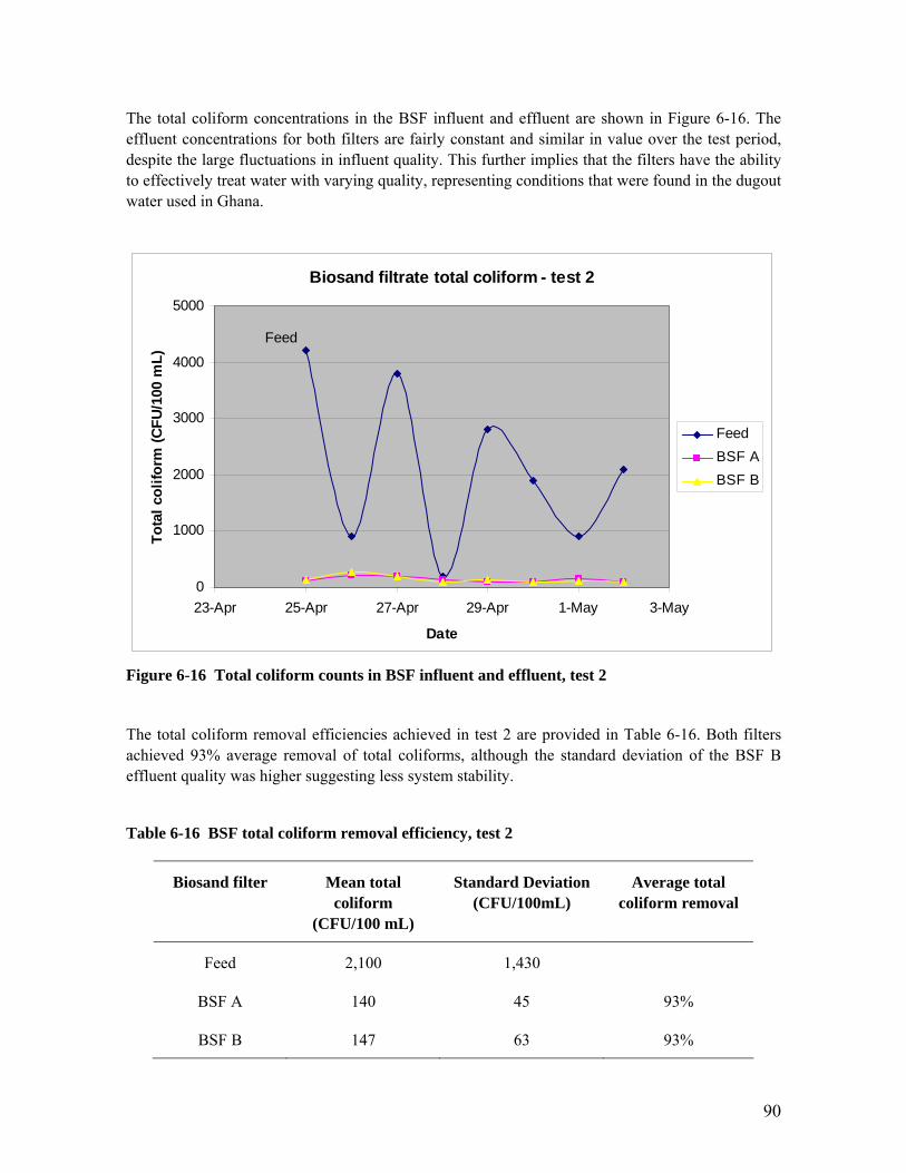
90

The total coliform concentrations in the BSF influent and effluent are shown in Figure 6-16. The effluent concentrations for both filters are fairly constant and similar in value over the test period, despite the large fluctuations in influent quality. This further implies that the filters have the ability to effectively treat water with varying quality, representing conditions that were found in the dugout water used in Ghana.

Biosand filtrate total coliform - test 2

0

1000

2000

3000

4000

5000

23-Apr 25-Apr 27-Apr 29-Apr 1-May 3-May

Date

Tota

l col

iform

(CFU

/100

mL)

FeedBSF ABSF B

Feed

Figure 6-16 Total coliform counts in BSF influent and effluent, test 2

The total coliform removal efficiencies achieved in test 2 are provided in Table 6-16. Both filters achieved 93% average removal of total coliforms, although the standard deviation of the BSF B effluent quality was higher suggesting less system stability.

Table 6-16 BSF total coliform removal efficiency, test 2

Biosand filter Mean total coliform

(CFU/100 mL)

Standard Deviation (CFU/100mL)

Average total coliform removal

Feed 2,100 1,430

BSF A 140 45 93%

BSF B 147 63 93%

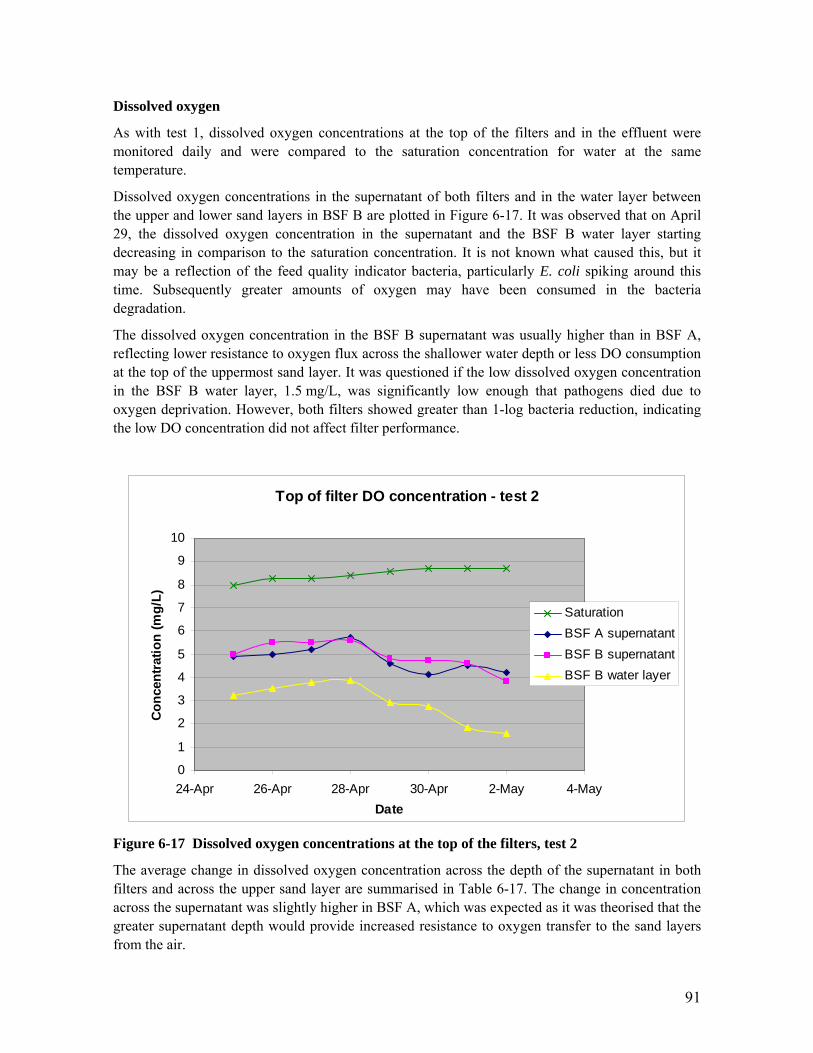
91

Dissolved oxygen

As with test 1, dissolved oxygen concentrations at the top of the filters and in the effluent were monitored daily and were compared to the saturation concentration for water at the same temperature.

Dissolved oxygen concentrations in the supernatant of both filters and in the water layer between the upper and lower sand layers in BSF B are plotted in Figure 6-17. It was observed that on April 29, the dissolved oxygen concentration in the supernatant and the BSF B water layer starting decreasing in comparison to the saturation concentration. It is not known what caused this, but it may be a reflection of the feed quality indicator bacteria, particularly E. coli spiking around this time. Subsequently greater amounts of oxygen may have been consumed in the bacteria degradation.

The dissolved oxygen concentration in the BSF B supernatant was usually higher than in BSF A, reflecting lower resistance to oxygen flux across the shallower water depth or less DO consumption at the top of the uppermost sand layer. It was questioned if the low dissolved oxygen concentration in the BSF B water layer, 1.5 mg/L, was significantly low enough that pathogens died due to oxygen deprivation. However, both filters showed greater than 1-log bacteria reduction, indicating the low DO concentration did not affect filter performance.

Top of filter DO concentration - test 2

0

1

2

3

4

5

6

7

8

9

10

24-Apr 26-Apr 28-Apr 30-Apr 2-May 4-MayDate

Con

cent

ratio

n (m

g/L)

SaturationBSF A supernatantBSF B supernatantBSF B water layer

Figure 6-17 Dissolved oxygen concentrations at the top of the filters, test 2

The average change in dissolved oxygen concentration across the depth of the supernatant in both filters and across the upper sand layer are summarised in Table 6-17. The change in concentration across the supernatant was slightly higher in BSF A, which was expected as it was theorised that the greater supernatant depth would provide increased resistance to oxygen transfer to the sand layers from the air.

92

The change in dissolved oxygen concentration across the upper sand layer of BSF 2 was significantly less than across the supernatant of the same filter. This was not expected as the sand was expected to increase the change in concentration by limiting diffusion to pore spaces.

Table 6-17 Change in dissolved oxygen concentrations across the top of the filters, test 2

Biosand filter Average DO concentration change in supernatant (mg/L)

(Standard deviation)

Average DO concentration change in upper sand layer (mg/L)

(Standard deviation)

BSF A 3.7 (0.7)

BSF B 3.5 (0.8) 2.0 (0.3)

The dissolved oxygen concentrations in the BSF filtrate are provided in Figure 6-18, although measurements were not taken on all test days. From this figure, it can be seen that the dissolved oxygen concentration in BSF A effluent is lower than that in BSF B, suggesting greater consumption of oxygen occurred in BSF A. This could be a result of the continuous uppermost sand layer in BSF A supporting a greater unbroken depth of sand for biofilm adherence.

The dissolved oxygen concentrations are very low, suggesting pathogen death by starvation may have occurred in the filters.

Filtrate DO concentration - test 2

0.0

0.5

1.0

1.5

2.0

23-Apr 25-Apr 27-Apr 29-Apr 1-May 3-May

Date

Conc

entra

tion

(mg/

L) BSF ABSF B

Figure 6-18 Dissolved oxygen concentrations in the filtrate, test 2

93

Table 6-18 shows the average change in dissolved oxygen concentration across the sand layers for both of the filters. For BSF B the value represents the change in concentration between the top of the upper sand layer and the filtrate, and for BSF A it is the concentration change between the top of the single sand layer and the filtrate.

The change in DO, due to diffusion capacity through the sand and consumption by micro-organisms, was lower in BSF A, suggesting less oxygen was consumed in this filter. However, based on similar indicator bacteria removal performance the difference in dissolved oxygen profiles across the filter does not appear to be a restraint on filter performance.

Table 6-18 Change in dissolved oxygen concentrations across the BSF sand layers, test 2

Biosand filter Average DO concentration change across sand (mg/L)

(Standard deviation)

BSF A 3.7 (0.7)

BSF B 3.9 (0.5)

Summary

The following key observations were made during test 2:

• Short-circuiting was not considered to be a major cause of difference in flow rate between the two filters

• The schmutzdecke was not considered to be the cause of the difference in the filter flow rates

• BSF B, the dual sand layer BSF, performed slightly better for microbial reductions

• The ripened filters managed fluctuations in feed quality effectively

• BSF B had higher DO concentration at the uppermost sand layer

• It was surmised that sufficient DO concentrations reached the lower sand layer in BSF B to support oxidation filtration

• The change in DO across the total sand depth of BSF B was greater than for BSF A. Considering that BSF B had a higher DO concentration at the uppermost sand layer it was inferred that more biological activity occurred in this filter.

94

6.3.4 Test 3 results Test 3 was used to assess the influence of two factors on BSF performance:

a. The effect on effluent quality due to increasing the filling cycle frequency to twice per day.

b. The effect on effluent quality when the feed water passes through the filter in one filling cycle. This was achieved by filling the filters with 20 L of source water, double the filter pore volume.

“swirl and dump” cleaning occurred the day prior to test 3 commencing and again on day 3 of the test.

Test 3a – Assessment of increasing feeding frequency In this test the filters were fed twice daily, at approximately 9am and 6pm. A total of 7 tests were conducted.

Flow rate

The flow rates of both the filters were recorded during three tests, immediately after 10 L of feed water had been poured into the filters. The flow rates were constant during this test and are shown in Table 6-19. As with other tests conducted during this BSF optimisation study, it was assumed the difference in the flow rates was a function of sand grain arrangement. Short-circuiting within the filter was ruled out as a gross cause in tests 1 and 2, and the influence of the schmutzdecke was discounted in test 2.

Table 6-19 BSF average flow rates, test 3

Biosand filter Flow rate (L/min)

BSF A 0.4

BSF B 0.7

Turbidity

The influent and effluent BSF turbidities are shown in Figure 6-19. The influent turbidity fluctuated across the test period, however, this was not reflected in the effluent turbidity, which remained stable after the first test reading. The first effluent reading (May 3) was the lowest taken during this test, reflecting the 24 hour pause time this water spent inside the filter during the transition from test 2 to test 3.

95

Biosand filtrate turbidity - test 3a

0

50

100

150

200

250

300

350

3-May 4-May 5-May 6-May 7-May

Date

Turb

idity

(NTU

)

FeedBSF ABSF B

Feed

Figure 6-19 BSF turbidity, test 3a

Table 6-20 shows the average turbidity removal statistics for the filters. This test was the only one of the three tests run using 10 L volume of feed water, in which the effluent turbidity rose above 6 NTU. It was noted in the control tests, as well as tests 1 and 2, that the turbidity removal of the filters was around 97 – 98%. It is likely that the increase in effluent turbidity in this test is a result of the shorter pause phase limiting the amount of sedimentation and adherence of particulates to the sand.

Table 6-20 BSF turbidity removal efficiency, test 3a

Biosand filter Mean turbidity (NTU)

Standard Deviation (NTU)

Average turbidity removal

Feed 183 62

BSF A 12 4 93%

BSF B 12 3 93%

Microbiological quality

For the feed water, all 3M Petrifilm tests returned counts for total coliform colonies. However, on two occasions E. coli counts were in the range 10 – 99 CFU/100 mL, that is no counts were recorded using the 3M Petrifilms and Colilert tests returned positive results. Membrane filtration

96

was not conducted for the feed water due to the high turbidity of the water making it had to sample by this method, and due to a limited quantity of m-ColiBlue24® Broth available in the laboratory. Therefore, based on sewage dosing quantities used to spike the feed water on other occasions, it is highly likely that the E. coli concentrations were close to 100 CFU/100 mL and so the value of 99 E. coli CFU/100 mL was assigned to these samples.

The effluent results presented are those gathered using the MF testing method as greater enumeration of colonies was achieved. The MF results and the 3M Petrifilm and Colilert test results were in basic agreement, validating the use of the MF results for effluent quality analysis in this section.

Figure 6-20 shows the E. coli removal efficiencies of the two BSFs. The introduction of fresh sewage on May 4 can be seen by the sharp increase in E. coli concentration on the same day, the effects of this on the effluent quality are discussed below.

Biosand filtrate E. coli - test 3a

-1000

0

1000

2000

3000

4000

5000

6000

3-May 4-May 5-May 6-May 7-May

Date

E. c

oli (

CFU/

100

mL)

FeedBSF ABSF B

Feed

Figure 6-20 E. coli counts in BSF influent and effluent, test 3a

Table 6-21 and Table 6-22 compare the average E. coli removal efficiencies of the two filters based on feed water spiked with old sewage and fresh sewage, respectively, as the E. coli source in the water.

With the introduction of the fresh sewage, the E. coli effluent concentrations increased by approximately 1-log, as shown in Table 6-22, however the E. coli removal efficiency of both filters increased to 2-log reduction. For both old sewage and fresh sewage spiked effluent conditions, the average E. coli removal efficiency was higher for BSF B, the dual sand layer BSF.

97

The fresh sewage was introduced on the evening filling session of May 4, however the increase in effluent E. coli was not observed until the next filling session carried out on the morning of May 5, due to retention in the pore volume.

Table 6-21 BSF E. coli removal efficiency, test 3a (old E. coli source)

Biosand filter Mean E. coli (CFU/100 mL)

Standard Deviation (CFU/100mL)

Average E. coli removal

Feed 170 116

BSF A 11 8 94%

BSF B 5 8 97%

Table 6-22 BSF E. coli removal efficiency, test 3a (fresh E. coli source)

Biosand filter Mean E. coli (CFU/100 mL)

Standard Deviation (CFU/100mL)

Average E. coli removal

Feed 4,330 520

BSF A 88 58 99%

BSF B 75 48 99%

Figure 6-21 shows the total influent and effluent coliform counts for this test. The introduction of the fresh sewage to the source water can be seen on May 4 by the rise in total coliform concentration.

98

Biosand filtrate total coliform - test 3a

-2000

0

2000

4000

6000

8000

10000

12000

3-May 4-May 5-May 6-May 7-May

Date

Tota

l col

iform

(CFU

/100

mL) Feed

BSF ABSF B

Feed

Figure 6-21 Total coliform counts in BSF influent and effluent, test 3a

Table 6-23 and

Table 6-24 show the average total coliform removal efficiencies for the BSFs for raw water spiked with old and fresh sewage, the source of the total coliform, respectively. Almost a 9-fold increase in the raw water total coliform concentration was observed due to the use of fresh sewage. However, this rise was not strongly reflected in the effluent, with the total coliform count in BSF A increasing by 50%, from 260 to 390 CFU/100 mL) and in BSF B by 3%, from 300 to 310 CFU/100 mL, during the second filling session using the fresh sewage. The ability of BSF B to remove total coliform from the water does not appear to be affected by the increase in the feed concentration given that the total coliform count in the effluent only rose by 3%.

As was observed with the E. coli removal results, greater total coliform removal efficiency was observed in both filters when the fresh sewage was used and the raw water total coliform concentration was higher. Using the old sewage source, BSF A showed higher total coliform removal efficiency, however, BSF showed higher efficiency with the fresh sewage source.

Table 6-23 BSF total coliform removal efficiency, test 3a (old E. coli source)

Biosand filter Mean E. coli (CFU/100 mL)

Standard Deviation (CFU/100mL)

Average E. coli removal

Feed 1,030 650

BSF A 260 115 75%

99

BSF B 300 70 71%

Table 6-24 BSF total coliform removal efficiency, test 3a (fresh E. coli source)

Biosand filter Mean E. coli (CFU/100 mL)

Standard Deviation (CFU/100mL)

Average E. coli removal

Feed 9,100 365

BSF A 390 115 96%

BSF B 310 110 97%

Dissolved oxygen

Dissolved oxygen concentrations in the filters were recorded at each filling session. The concentration at the top of the filters was measured prior to filling the filter and the effluent concentration was measured at the same time the effluent quality was monitored for turbidity and microbiological quality, after approximately 5 L of effluent had been collected.

The dissolved oxygen concentrations in the top of the filters are compared to the saturation concentration for the relevant water temperature in Figure 6-22.

The dissolved oxygen concentration at the surface of the upper sand layer in BSF B is slightly lower than for BSF A at most data points, contrasting to results from tests 1 and 2. The first test conducted on May 5, during the first filling cycle after the introduction of fresh sewage to spike the feed water, the dissolved oxygen concentrations in the top of the filters started to increase. It was thought that this would decrease due to a greater amount of bacteria and other organic matter in the water using more oxygen in the oxidation filtration process, that is to say it was expected the biochemical oxygen demand of the system would increase. However, as both the E. coli and total coliform removal efficiencies increased at the introduction of the fresh sewage, it was inferred that the increase in dissolved oxygen concentrations did not adversely affect filter performance.

100

Top of filter DO concentration - test 3a

0

1

2

3

4

5

6

7

8

9

10

3-May 4-May 5-May 6-May 7-MayDate

Con

cent

ratio

n (m

g/L)

SaturationBSF A supernatantBSF B supernatantBSF B water layer

Figure 6-22 Dissolved oxygen concentrations at the top of the filters, test 3a

The change in dissolved oxygen concentration across the depth of the supernatant for both filters and across the upper sand layer for BSF B is shown in Table 6-25.

As the test progressed the change in dissolved oxygen concentration across the upper sand layer of BSF B decreased, also seen in Figure 6-22, indicating more oxygen was reaching the lower sand layer and thereby providing greater support for biological activity in the lower sand layer.

As shown in Table 6-25, the change in concentration across the supernatant was roughly double that across the upper sand layer in BSF B. Considering that the upper sand layer depth of 3 cm was slightly larger than that of the supernatant, 2.5 cm, and that dissolved oxygen flux through the upper sand layer is limited to the pore space, it was surprising that the dissolved oxygen change across the supernatant layer was so high. It is not known why this occurred.

Table 6-25 Change in DO concentration across the top of the filters, test 3a

Biosand filter Average DO concentration change in supernatant (mg/L)

(Standard deviation)

Average DO concentration change in upper sand layer (mg/L)

(Standard deviation)

BSF A 3.8 (0.8)

BSF B 4.0 (0.6) 1.8 (0.7)

101

Figure 6-23 shows the dissolved oxygen concentrations in the BSF effluent during test 3a, a value for BSF A was not recorded on the morning of May 5. Both filters show similar effluent concentrations, which reflect the dips and rises also seen in the dissolved oxygen concentrations at the top of the filter (see Figure 6-22), suggesting a constant amount of oxygen was consumed in each filter during the test period.

Filtrate DO concentration - test 3a

0

1

2

3

4

3-May 4-May 5-May 6-May 7-May

Date

Conc

entra

tion

(mg/

L) BSF ABSF B

Figure 6-23 Dissolved oxygen concentrations in the filtrate, test 3a

The average change in dissolved oxygen concentration across the filter, from the top of the uppermost sand layer to the effluent, is shown in Table 6-26. Less dissolved oxygen was consumed in BSF B, suggesting less oxidation filtration of the feed water occurred. The higher dissolved oxygen removal in BSF A may be a result of the continuous sand layer in BSF A providing a greater sand depth on which biofilm could be supported and therefore a greater capacity for oxidation filtration to occur, however, this theory is not supported by the similar E. coli and total coliform removal efficiencies of the two filters.

Table 6-26 Change in dissolved oxygen concentration across the BSF sand layers, test 3a

Biosand filter Average DO concentration change across sand (mg/L)

(Standard deviation)

BSF A 2.5 (0.7)

BSF B 1.9 (0.7)

102

Summary

The following key observations were made during test 3a:

• Effluent turbidity was affected by pause time

• Increased filling frequency led to higher microbial effluent concentrations but also higher microbial removal efficiency

• BSF B, the dual sand layer BSF, performed slightly better for E. coli reductions

• When fresh sewage was used to source indicator organisms, and higher bacteria concentrations were present, the DO concentrations in the BSF A and B supernatant and BSF B water layer increased

• BSF B had lower DO concentration at the uppermost sand layer

• Surmised that sufficient DO concentrations probably reached the lower sand layer in BSF B to support oxidation filtration

Test 3b – Assessment of increasing feed volume above pore volume In this test the filters were fed twice daily on the first day of the test and once daily for the remaining 3 days of the test. A total of 5 tests were conducted. Each filter was filled with 20 L of turbidity and indicator bacteria spiked water. Effluent quality measurements were recorded when 15 L of effluent had been collected. The filtrate flow rate was not measured as part of this test due to time constraints, although it was expected to have increased at the beginning of the filling cycle due to the increased pressure head caused by the greater volume of water poured into the filter.

Turbidity

The influent and effluent BSF turbidities are shown in Figure 6-24. The influent turbidity fell throughout the study, a result of inconstant clay spiking of the feed water. It was observed that the effluent turbidities for both of filters was fairly constant around 50 NTU for all test results, and they did not reflect the fall in feed turbidity.

103

Biosand filtrate turbidity - test 3b

0

50

100

150

200

250

300

350

3-May 4-May 5-May 6-May 7-MayDate

Turb

idity

(NTU

)

FeedBSF ABSF B

Feed

Figure 6-24 BSF turbidity, test 3a

Table 6-27 shows the average turbidity removal statistics for the filters. The results show the BSF A achieved slightly better turbidity removal at 76%, compared to 74% in BSF B.

Table 6-27 BSF turbidity removal efficiency, test 3b

Biosand filter Mean turbidity (NTU)

Standard Deviation (NTU)

Average turbidity removal

Feed 193 71

BSF A 46 12 76%

BSF B 51 12 74%

The BSF effluent turbidity achieved in this test was then compared to that achieved in test 3a, to observe the effect on water quality when the feed passed through the filter in the same filling cycle. These tests were run at the same time with the same feed water and therefore the same feed turbidity. 20 L of feed was poured into the filter and test 3a results read when 5 L of filtrate had been collected and test 3b results when 15 L of filtrate had been collected. The turbidity removal efficiencies are compared in Table 6-28.

From the comparison it was observed that turbidity removal efficiency dropped significantly in test 3b, when the feed water passed through the filter in the same filling cycle. It is mostly likely this is

104

due to the reduced time for particulate sedimentation and adherence to the sand grains and biofilm in the filter and reduced time for pathogen predation.

Table 6-28 Comparison of turbidity removal efficiencies in tests 3a and 3b

Biosand filter Test 3a - average turbidity removal

Test 3b - average turbidity removal

BSF A 93% 76%

BSF B 93% 74%

Microbiological quality

The same feed water was used in this test as for test 3a, and as such one of the two E. coli test results that fell in the range 10 – 99 CFU/100 mL was part of this test and 99 E. coli CFU/100 mL was likewise assigned to this sample. Again, membrane filtration of the feed water was not undertaken due to the high water turbidity and the limited supply of m-ColiBlue24® Broth.

The effluent results presented are those gathered using the MF testing method as greater enumeration of colonies was achieved. The MF results and the 3M Petrifilm and Colilert test results were in basic agreement, validating the use of the MF results for effluent quality analysis in this section. The only exception to this was the BSF B total coliform MF test conducted on May 6, for which the colonies were too small to count, and the 3M Petrifilm enumeration of the total coliform results was used instead.

The E. coli influent and effluent concentrations for the two filters are shown in Figure 6-25. The addition of fresh sewage to the feed water can be seen on May 4, and the resulting increase in effluent E. coli concentrations is reflected on the same day reflecting the effluent passing through the filter in one filling cycle.

105

Biosand filtrate E. coli - test 3b

-1000

0

1000

2000

3000

4000

5000

6000

3-May 4-May 5-May 6-May 7-May

Date

E. c

oli (

CFU

/100

mL)

FeedBSF ABSF B

Feed

Figure 6-25 E. coli counts in BSF influent and effluent, test 3b

Table 6-29 and Table 6-30 compare the average removal efficiencies of the two filters based on feed water spiked with old sewage and fresh sewage, respectively, as the E. coli source in the water.

Both filters show greater than 75% E. coli removal from the feed water through filling stage filtration only, when the old sewage was used to provide the indicator bacteria. When the fresh sewage was introduced the removal efficiency dropped in both filters to around 50%, which is still a fair degree of contaminant reduction. This drop in performance may be a result of the filters not being sufficiently adjusted to the new feed conditions to effectively remove the bacteria. Given enough time to mature for the new feed conditions the filter performance may have improved. However, as filter performance improved in test 3a with the addition of fresh sewage, this theory was discredited, It most likely that the feed bacteria concentrations were too high for the filter to effectively treat.

Table 6-29 BSF E. coli removal efficiency, test 3b (old E. coli source)

Biosand filter Mean E. coli (CFU/100 mL)

Standard Deviation (CFU/100mL)

Average E. coli removal

Feed 200 142

BSF A 48 11 76%

BSF B 45 35 78%

106

Table 6-30 BSF E. coli removal efficiency, test 3b (fresh E. coli source)

Biosand filter Mean E. coli (CFU/100 mL)

Standard Deviation (CFU/100mL)

Average E. coli removal

Feed 4,530 379

BSF A 2,230 630 49%

BSF B 2,120 347 53%

The E. coli removal efficiencies of the filters during this test were then compared to the removal efficiencies achieved in test 3a, where the water had rested the filter for a minimum 9 hour pause phase. The filter performances for the two tests, 3a and 3b, are shown in Table 6-31 for the old sewage spiked feed and Table 6-32 for the fresh sewage spiked feed.

It was observed that the removal efficiencies are lower for both sewage sources in test 3b, as was expected, as the feed water in test 3b had not been treated by the pause phase of the filtration cycle.

Table 6-31 E. coli removal efficiencies in tests 3a and 3b (old E. coli source)

Biosand filter Test 3a - average E. coli removal

Test 3b - average E. coli removal

BSF A 94% 76%

BSF B 97% 78%

Table 6-32 E. coli removal efficiencies in tests 3a and 3b (fresh E. coli source)

Biosand filter Test 3a - average E. coli removal

Test 3b - average E. coli removal

BSF A 99% 49%

BSF B 99% 53%

Figure 6-26 shows the influent and effluent total coliform concentrations for BSFs A and B for test 3b. As with the E. coli concentrations, the influence of the fresh sewage total coliform concentration can be seen on May 4 in both the influent and the effluent, reflecting the feed volume greater than the pore volume of the filters.

107

Biosand filtrate total coliform - test 3b

0

2000

4000

6000

8000

10000

3-May 4-May 5-May 6-May 7-May

Date

Tota

l col

iform

(CFU

/100

mL)

FeedBSF ABSF B

Feed

Figure 6-26 Total coliform counts in BSF influent and effluent, test 3b

Table 6-33 and Table 6-34 show the average total coliform removal efficiencies for the BSFs for raw water spiked with old and fresh sewage, the source of the total coliform, respectively. The total coliform removal efficiencies were different for the two filters under both feed conditions. The ability of BSF A to removal total coliform increased with the addition of fresh sewage, while the performance of BSF B decreased. It is not known why this occurred, especially as this was not reflected in the filters’ ability to reduce E. coli concentration. The final data point for BSF B is that read from 3M Petrifilm results, and represents the largest deviation in performance between the two filters, perhaps as a result of the different testing methods.

Table 6-33 BSF total coliform removal efficiency, test 3b (old total coliform source)

Biosand filter Mean total coliform (CFU/100 mL)

Standard Deviation (CFU/100mL)

Average total coliform removal

Feed 1,350 495

BSF A 690 68 49%

BSF B 400 346 70%

108

Table 6-34 BSF total coliform removal efficiency, test 3b (fresh total coliform source)

Biosand filter Mean total coliform (CFU/100 mL)

Standard Deviation (CFU/100mL)

Average total coliform removal

Feed 8,970 306

BSF A 3,010 550 66%

BSF B 3,760 1339 58%

As for the E. coli results, the total coliform removal efficiencies of the filters during this test were compared to the removal efficiencies achieved in test 3a, where the water had rested the filter for a minimum 9 hour pause phase. The filter performances for the two tests, 3a and 3b, are shown in Table 6-31 for the old sewage spiked feed and Table 6-32 for the fresh sewage spiked feed.

It was observed that the removal efficiencies are lower for both sewage sources in test 3b, except for BSF B fed with old sewage which showed approximately the same removal efficiency around 70%. This high removal efficiency in BSF B was not expected as the water had not been treated during a pause phase and it is possible that erroneous results led to this high performance being shown. For all other tests the lower filter performance for treatment of water during the filling cycle only was expected.

Table 6-35 Total coliform removal efficiencies in tests 3a and 3b (old total coliform source)

Biosand filter Test 3a - average total coliform removal

Test 3b - average total coliform removal

BSF A 75% 49%

BSF B 71% 70%

Table 6-36 Total coliform removal efficiencies in tests 3a and 3b (fresh total coliform source)

Biosand filter Test 3a - average total coliform removal

Test 3b - average total coliform removal

BSF A 96% 66%

BSF B 97% 58%

109

Dissolved oxygen

Dissolved oxygen concentrations in the filters were recorded at each filling session. As tests 3a and 3b were run together, the dissolved oxygen concentration at the top of the filters was the same measurement for both tests and is presented as part of test 3a.

The dissolved oxygen concentration of the filter effluent for test 3b was measured when 15 L of filtrate had been collected. Figure 6-27 shows the effluent concentrations for the two filters. There is good agreement between the filter effluent dissolved oxygen concentrations for all tests except that taken on the evening of May 5. It is not known what caused this difference in the data points, but as the surrounding data points show similar dissolve oxygen concentrations it is possible that there was error in the results. Apart from the anomaly in the results on May 6, the effluent dissolved oxygen concentrations are fairly constant at 5.0 mg/L for the duration of the test and do not reflect the switch from old to fresh sewage, indicating that a constant amount of oxygen was consumed during the filling phase.

Filtrate DO concentration - test 3b

0.0

1.0

2.0

3.0

4.0

5.0

6.0

3-May 4-May 5-May 6-May 7-May

Date

Conc

entra

tion

(mg/

L) BSF ABSF B

Figure 6-27 Dissolved oxygen concentrations in the filtrate, test 3b

The average change in dissolved oxygen concentration across the filter is shown in Table 6-37. For this test the change in concentration was taken as the difference between the saturation concentration of the feed water and the effluent concentration, as no pause phase had occurred.

The change in dissolved oxygen concentration was greater for BSF B, however, Figure 6-27 shows similar effluent values for all test occasions except May 6, when results considered to be anomalies were recorded. The larger change in dissolved oxygen concentration was a result of the different concentrations recorded on May 6.

110

Table 6-37 Change in dissolved oxygen concentrations across the BSF sand layers, test 3b

Biosand filter Average DO concentration change across sand (mg/L)

(Standard deviation)

BSF A 3.6 (0.5)

BSF B 4.0 (0.7)

Summary

The following key observations were made during test 3b:

• Effluent turbidity and microbiological quality was affected by fill volume exceeding pore volume

• BSF B, the dual sand layer BSF, performed slightly better for E. coli reductions

• Total coliform test results were mixed and inconclusive

• It was surmised that sufficient DO concentrations probably reached the lower sand layer in BSF B to support oxidation filtration of organisms that can easily be metabolised in the filter filling phase

6.4 Summary of optimisation test results As described in the previous section 6.3 and summarised in Table 6-4, the single sand layer and dual sand layer LPD BSFs were tested in the MIT laboratory under three sets of operating conditions to compare the performance of the two filters and measure the success of the modified BSF for treatment of high turbidity water, the dual sand layer BSF. The results of the three tests in terms of turbidity and indicator bacteria removal efficiency and dissolved oxygen concentration profiling are compared in this section.

Turbidity removal

Average turbidity removals achieved in the tests are compared below in Table 6-38. Comparing the performance of the two filters in all three tests, the removal efficiency of the single and dual sand layers was essentially the same.

Table 6-38 Comparison of BSF turbidity removal efficiency for the three tests

Biosand filter Test 1 Test 2 Test 3a Test 3b

BSF A 98% 99% 93% 76%

BSF B 98% 98% 93% 74%

111

Microbiological removal

The average E. coli removal achieved by the two test filters is summarised in Table 6-39. The influence of using old and fresh sewage as the source of E. coli is also shown. For all tests except test 2, the dual sand layer, BSF B, performed slightly better than the single sand layer system, implying this system has a greater capacity for E. coli removal under various conditions including disruption of any biological activity on the uppermost sand layer through the “swirl and dump” cleaning, increasing filling frequency and increasing filling volume beyond the pore volume of the filter.

Table 6-39 Comparison of BSF E. coli removal efficiency for the three tests

Biosand filter Test 1 Test 2 Test 3a

old / fresh

Test 3b

old / fresh

BSF A 75% 99% 94% / 99% 76% / 49%

BSF B 79% 98% 97% / 99% 78% / 53%

Table 6-40 summarises the average total coliform removal efficiency of the filters for the three tests. The effect of using old and fresh sewage as the source of total coliform is also shown. For tests 1 to 3a, the filters produced similar reduction capacities; however, the results for test 3b were mixed and inconclusive. It was surmised that both filters had equivalent capacities to operate under disturbances to the biological activity on the uppermost sand layer from the cleaning program and filling frequency conditions.

Table 6-40 Comparison of BSF total coliform removal efficiency for the three tests

Biosand filter Test 1 Test 2 Test 3a

old / fresh

Test 3b

old / fresh

BSF A 82% 93% 75% / 96% 49% / 66%

BSF B 85% 93% 71% / 97% 70% / 58%

Dissolved oxygen

The average change in dissolved oxygen across the supernatant, that is, the difference between the water saturation concentration and the measurement taken immediately above the uppermost sand layer, for both BSFs is shown in Table 6-41.

112

In tests 2 and 3, the change in consumption of dissolved oxygen, for both filters, is more than double the value observed during test 1. However, at the end of test 1, Figure 6-11 showed that the change in dissolved oxygen between the saturation value and the measurement at the sand surface increased, with the final value being 2.6 mg/L. Based on this, it was conjectured that the filters reached full maturation at the end of test 1.

The similar concentrations in both BSFs suggest that there was similar oxygen consumption in the filters causing the oxygen gradient across the supernatant, especially as the supernatant depth was similar for the two filters at 3.4 cm for BSF A and 2.7 cm for BSF B.

Table 6-41 Comparison of supernatant dissolved oxygen concentrations for the three tests

Biosand filter Test 1 (mg/L) Test 2 (mg/L) Test 3 (mg/L)

BSF A 1.4 3.7 3.8

BSF B 1.2 3.5 4.0

The steady state dissolved oxygen flux across the supernatant was then calculated, using Equation 3, based on the average change in dissolved oxygen concentration across the supernatant during tests 2 and 3. For both filters this was 3.75 mg/L dissolved oxygen. The average temperature of the water in the filters was 23°C. The diffusivity, Dm of oxygen in water is 2.10 cm2/s (2.10*10-4 m2/s) at 25°C (CRC, 1990) and the gas exchange coefficient, K, is 0.32 cm/hour at 20°C (Buzunis, 1995, from Haney, 1954), or 8.9*10-3 m/s. For BSF A the supernatant depth, z, was 3.4 cm, and for BSF B, was 2.7 cm. The oxygen flux, J, for each filter was calculated:

( )sandsatm

m CCDKzKD

J −+

−=

BSF A:

( ) ( )

( )( ) ( ) ( )( )smmgJ

mLLmgsmmsm

smsmJ

⋅−=

×××+×

×××−= −−

−−

2

3243

324

/14

/1000/75.3/1010.2034.0/109.8

/109.8/1010.2

BSF B:

( ) ( )( )( ) ( ) ( )

( )smmgJ

mLLmgsmmsm

smsmJ

⋅−=

×××+×

×××−= −−

−−

2

3243

324

/15

/1000/75.3/1010.2027.0/109.8

/109.8/1010.2

The flux across BSF B was greater, due to the shallower supernatant depth providing less resistance to mass transfer.

The average change in dissolved oxygen across the upper sand layer in BSF B for the three tests is shown in Table 6-42. As the BSFs were considered to have ripened at the end of test 1, the average

113

change in oxygen concentration across the upper sand layer was estimated from tests 2 and 3 as 1.9 mg/L. The average dissolved oxygen concentration in the BSF B water layer is also shown in Table 6-42. Assuming the minimum dissolved oxygen requirement for biological activity is 1 mg/L as mentioned by Buzunis (1995), then for all tests there was sufficient dissolved oxygen reaching the BSF B lower sand layer.

Table 6-42 Change in dissolved oxygen concentration across DSL BSF upper sand layer

Biosand filter Test 1 (mg/L) Test 2 (mg/L) Test 3 (mg/L)

Water layer concentration 5.6 2.9 2.9

Change concentration across upper sand layer

1.3 2.0 1.8

The oxygen flux through the upper sand layer was then calculated using Equation 6. For this, the dissolved oxygen concentration in the water layer between the upper and lower sand layers was assumed to be approximately equal to the dissolved oxygen concentration at the base of the upper sand layer. In section 6.1.2, it was theorised that the coarse sand layer would be the diffusion limiting layer, and as such the following calculations are based on the porosity of the coarse sand, 0.3.

Firstly, solving Equation 5, to adjust porosity value for flow tortuosity through the sand, where m = 2:

3.03.0 12

1

==

=−

−

nn

nn m

Solving Equation 4 for oxygen diffusivity through the coarse sand:

( )( )

smD

smD

nnDD

m

m

mm

/103.6'

3.0/1010.2'

'

25

24

−

−

×=

××=

=

The theoretical dissolved oxygen flux through the upper sand layer was then estimated with Equation 6, using the average change in concentration across the upper sand layer for tests 2 and 3:

( )( ) ( )

( )smmgJm

mLLmgsmJ

zCC

nDJ persandbottomofupsandtopofupperm

⋅−=

×⋅×−=

−−=

−

2

325

/2.103.0

/1000/9.13.0103.6

'

114

It was assumed from Table 6-42, that sufficient dissolved oxygen was reaching the BSF B lower sand layer and as such the calculated flux, 1.2 mg/(m2.s) should be sufficient to support biologically activity in the lower sand layer.

Table 6-43 shows the average change in dissolved oxygen concentration between the top of the uppermost sand layer and the outlet. This represents the oxygen consumption in the filters. There does not appear to be a clear delineation of which filter used more oxygen. This may be a reflection of the single sand layer BSF having deeper continuous sand media for biofilm adherence and/or the formation of a schmutzdecke layer on the lower sand layer of BSF B.

Table 6-43 Change in dissolved oxygen concentration across BSF depth of sand

Biosand filter Test 1 (mg/L) Test 2 (mg/L) Test 3a (mg/L) Test 3b (mg/L)

BSF A 2.9 3.7 2.5 3.6

BSF B 2.9 3.9 1.9 4.0

6.5 Discussion

6.5.1 DSL BSF performance Comparing the performance of the two BSFs in this optimisation study:

• the dual sand layer BSF performed slightly better in terms of indicator bacteria removal

• the two filters performed comparably in terms of turbidity removal

Comparing the results of tests 1 and 2, the 3-day cleaning program did not appear to have adverse effects on the quality of the filtrate. However, as the BSFs were determined to have ripened only at the end of test 1, further testing of these scenarios should be conducted to confirm the results.

The effect of pause time studied in test 3a, showed that effluent quality both in terms of turbidity and microbiological concentrations decreased with pause time shortened from 24 hours to 9 hours.

In test 3, the switch from old sewage to fresh sewage as the source of indicator bacteria, and the subsequent increase in feed bacteria concentration led to increased bacteria concentrations in the effluent. However, for test 3a, it was observed that the removal efficiencies increased.

The doubling of the fill volume in test 3b, such that a volume of water greater than the filter pore volume was poured into the filter during a filling cycle led to a notable decrease in effluent quality, both for turbidity and indicator bacteria concentrations.

The performance of the dual sand layer laboratory filter is compared to the field filter performance in Table 6-44. For the laboratory filter, the results of test 2 are used for the comparison. The test 1 method was more similar to the testing regime carried out in Ghana, but as the laboratory filters ripened only at the end of test 1, this was not considered representative of the test conditions in Tamale.

115

Table 6-44 Comparison of laboratory and field DSL BSF performance

Biosand filter Flow rate (L/min)

Turbidity removal

E. coli removal Total coliform removal

Field (BSF 2) 0.2 59% 85% 95%

Lab (BSF B) 0.7 98% 98% 93%

The laboratory filter performed better than the field filter for flow rate, turbidity removal and E. coli removal. Only the total coliform removal was higher in the field tested filter. Considering the issues with turbidity spiking the feed water in the laboratory it is difficult to compare the two filters for turbidity performance. It is also likely that the turbidity performance influenced the microbial reduction performance in Ghana by hindering contact between the biofilm and the pathogens.

The laboratory filter had a much faster flow rate, as a result of increasing the filter freeboard and therefore the water pressure head.

6.5.2 Estimated cost of DSL BSF The local plastic design DSL BSF proposed in this study requires two parts in addition to all parts used in the Kanchan™ style LPD BSF:

1. Additional diffuser basin as upper sand layer support base

2. Additional coarse sand for upper sand layer, approximately 2 L

As the DSL BSF lower fine sand layer is of a lesser depth than in a single sand layer LPD BSF, no additional fine sand is required for the DSL BSF.

The equipment cost of the DSL BSF, was estimated from LPD BSF component costs (2008 values) in Tamale, Ghana, reported by Kikkawa (2008), outlined in Table 6-45.

Table 6-45 Dual sand layer BSF estimated cost

Item Quantity Cost ($USD, 2008)

Diffuser basin 1 $1.00

Coarse sand 2 L $0.521

LPD BSF 1 $16.15

Total 1 $17.67

1 – Estimated from the cost of 4 L coarse sand, $1.04.

116

The cost of the DSL BSF ($17.67) is 9% higher than the LPD BSF constructed by Kikkawa. Compared to BSF costs provided in Table 3-1, the DSL BSF cost is comparable to the CAWST style concrete BSF ($12 - $30) and the LPD BSF ($15 - $20). The International Aid HydrAid™ BSF is still a significantly more expensive filter ($75). Economically, the DSL BSF is a viable option for water treatment using biosand filtration technology, providing a technology that is potentially affordable to locals and sustainable.

6.5.3 Recommendations It is recommended that the dual sand layer biosand filter be studied further. In the laboratory study, testing was limited due to the failure to recreate turbid water similar to that found in dugouts in northern Ghana.

A microbially-compromised source water, more representative of that found in dugouts should be applied in future studies. The use of the Charles River for water and the addition of sewage for indicator bacteria may not have truly represented the quality of dugout water and further field investigations with dugout water should be conducted. In particular, testing with higher turbidity water, as has been recorded in Tamale, Ghana, should be conducted to investigate the efficiency of the DSL BSF under extremely high turbidity conditions.

The 3-day cleaning program did not appear to have a significant impact on the filtrate quality, although theoretically it can be expected to have some impact. Longer duration studies should investigate the effects of the “swirl and dump” cleaning method on the filtrate of both single and dual sand layer biosand filters as beneficial in future design optimisations.

Experiments with the depth and layout of the upper sand layer in the DSL BSF can lead to further system optimisation. Increasing the flux though the upper sand layer will allow more oxygen to flow through to the lower sand layer, and therefore a greater degree of biological activity could operate in the lower sand layer. Key design focal points for optimising the oxygen flux are the upper sand layer, supernatant and water layer depths, and the porosity of the upper sand layer.

The effect of reducing the depth of the lower sand layer to allow the DSL BSF to fit into a Kanchan™ filter unit should be further investigated to identify any impacts on the filtrate quality.

Rigorous testing of the DSL BSF in the field is highly recommended, together with single sand layer BSF testing, to compare the dual sand layer system performance.

It should be noted that this design is not restricted to BSFs with plastic shells; an upper sand layer could be incorporated into the concrete design. An additional concrete step could be added to the design on which the support plate would rest. The support plate should be equipped with extended handles (above the supernatant top water level) to allow removal of the support plate and cleaning of the lower sand layer as required.

117

7. Safe Storage for BSF Filtrate This study also addressed safe storage of the BSF filtrate, in order to mitigate recontamination of the water. Identifying safe storage options for the BSF filtrate involved three methods of investigation:

1. Field monitoring of filtrate quality over time in both clean and unclean storage vessels.

2. Field observations of BSF operation and storage practices by local people in Tamale.

3. Discussion of safe storage options with Community Water Solutions, an organisation providing safe water storage vessels in the Tamale region.

7.1 Filtrate quality monitoring in local storage vessels During January 2009, experiments were conducted to measure the quality of BSF filtrate stored in 20 L plastic jerry cans, as shown in Figure 7-1. Jerry cans are typically left over from the transportation of palm oil and are frequently cleaned then used as water transfer and storage vessels in the Tamale area as well as in many other developing regions in the world.

Figure 7-1 Jerry cans used for water storage (Source: Collin, 2009)

Two jerry cans used by the PHW office to collect dugout water were used to compare the quality of filtrate over time. One jerry can was disinfected with household bleach prior to filling with filtrate and the other jerry can, which had been used for collecting dugout water for filling the BSFs, was not cleaned and remained contaminated with dugout water. The filtrate used to fill the jerry cans was taken from the modified BSF 1, ensuring that the filtrate quality entering the two vessels was the same. The jerry cans were filled over two BSF filling sessions conducted within several hours of each other, with each jerry can half-filled during each session. Both storages vessels were kept in a shaded location to prevent algal growth or damage to the plastic from UV sun rays.

118

The quality of the filtrate was then monitored over a period of time for turbidity and microbiological quality (E. coli and total coliform). The stored filtrate was not mixed during this time. Only one complete test comparing the two storage methods was completed. The testing methods used for determining storage vessel E. coli and total coliform concentrations with 3M Petrifilm and Colilert tests are detailed in Section 5.3.1 Test procedures.

Turbidity

The turbidity of the filtrate supernatant decanted from each jerry can is shown in Figure 7-2.

The disinfected jerry can shows an initial turbidity much lower than the feed but which increases over the elapsed storage time. The initial reduction in turbidity is most likely due to sedimentation; however, the reason for the increase in turbidity is uncertain.

In contrast to the filtrate quality seen in the disinfected jerry can, the dirty jerry can shows an initial rise in turbidity, above the feed turbidity, which then drops off. The cause of the initial increase in turbidity is probably a result of stirring up sedimentation or biofilm that existed in the jerry can prior to filling with filtrate. The fall in turbidity is possibly the result of the stirred-up sediments resettling.

Jerry can storage turbidity

84

86

88

90

92

94

96

98

100

0 10 20 30 40 50 60Elapsed storage time (hours)

Turb

idity

(NTU

) BSF filtratefeed

Disinfectedjerry can

Dirty jerrycan

Figure 7-2 Jerry can storage turbidity

119

Microbiological quality

Figure 7-3 shows E. coli concentrations in the two jerry cans against the feed concentration over the test period. While the disinfected jerry can showed increased E. coli concentration immediately after filling, the concentration decreased rapidly over the first three hours of storage, a likely result of chlorine residual disinfection in the vessel. After a day of storage the E. coli concentration in the disinfected jerry can began to increase indicating growth of bacteria.

As was seen in the total coliform test results, the initial E. coli concentration in the dirty jerry can doubled the feed concentration after 3 hours, probably due to the addition of contamination pre-existing in the vessel. The concentration of the E. coli then decreased to below that of the disinfected jerry can after 24 hours and remained below the disinfected jerry can after 48 Hours as well.

Jerry can storage E. coli concentrations

0

100

200

300

400

500

600

700

800

0 10 20 30 40 50 60Elapsed storage time (hours)

Mic

robi

al c

ount

(CFU

/100

mL)

BSF filtratefeed

Disinfectedjerry can

Dirty jerry can

Figure 7-3 Jerry can storage E. coli concentrations

A comparison of the total coliform concentrations in the two jerry cans against the feed concentration is provided in Figure 7-4.

The disinfected jerry can showed an initial dip in total coliform concentration, most likely a result of coliform bacteria die-off due to residual chlorine in the vessel from the bleach used to the jerry can. As time elapsed the total coliform concentration increased above the feed concentration as the residual chlorine was exhausted and coliform units began to proliferate.

The dirty jerry can showed an erratic total coliform concentration profile over the sample period. The two samples taken within three hours of filling show the total coliform concentration double that of the feed, most likely due to coliform contamination pre-existing in the jerry can. A dip in

120

concentration one day later could be the result of bacteria die-off due to competition for oxygen and nutrients or a sampling error. The final test shows high coliform contamination closer in value to the earlier tests, suggesting the much lower coliform value may have been erroneous.

Jerry can storage total coliform concentrations

0

200400

600

800

10001200

1400

16001800

2000

0 10 20 30 40 50 60

Elapsed storage time (hours)

Mic

robi

al c

ount

(CFU

/100

mL)

BSF filtratefeed

Disinfectedjerry can

Dirty jerrycan

Figure 7-4 Jerry can storage total coliform concentrations

Both the turbidity and microbiological test results indicate that the disinfected jerry can improved water quality initially but that it degraded over time. In contrast, the water quality in the dirty jerry can initially worsened but improved over the test period such that it was better than the quality of the filtrate in the disinfected jerry can. The improvement in filtrate quality in the dirty jerry can was not expected and further testing should be undertaken to confirm the results of this study.

7.2 Field observations of filtrate storage practices Batamyili village, Savelugu

On January 23, 2009, Batamyili village, near Savelugu to the north of Tamale, was visited at the invitation of Issaka Balima Musah of the E.U./UNICEF Integrated Water, Sanitation and Hygiene (I-WASH) Project to sample the water quality of International Aid HydrAid™ BSFs installed in the village. Approximately 100 BSFs had been distributed, of which 25 were sampled; water quality results are provided in Appendix B and discussed in section 3.3.2. As part of this testing, the filtrate storage practices of the villagers was observed.

At the 25 households visited with filters, the filter users indicated that due to the high flow rate of the filter (1 L/min average), the filter was used on an “as needed” basis. That is to say, water was not filtered and stored for later use. Only two households had any form of filtrate storage and the quality of the filtrate was measured. The results of one of the samples was lost, and the other sample

121

indicated stored water quality approximately the same as the BSF filtrate for turbidity, total coliform and E. coli readings.

All of the households collected the filtrate in a wide-mouthed pot, bucket or garawa (large tin can), as shown in Figure 7-5. In Figure 7-5a, the collection bucket lid can be seen on top of the filter. Only nine of the 25 filter users could produce a lid for the collection vessel upon request. Frequently, young children and animals were witnessed in the same room where the filter was kept, providing a potential source of filtrate contamination.

Figure 7-5 BSF filtrate collection vessels: a) plastic bucket with lid and b) garawa (Source: Collin, 2009)

Zuozugu village, Tamale

On January 20, 2009, four households in Zuozugu village, on the outskirts of Tamale, who had received International Aid HydrAid™ BSFs were visited. One of the filter users caught the filtrate in jerry cans, one in a tin can and the other two in buckets, for which only one had a lid. Only the household that collected filtrate in a tin can indicated that filtrate was stored for future use. In this case the filtrate was transferred to a jerry can for her husband to take with him to work in the fields. Additional information on the water quality is provided in Appendix C and discussed in Section 3.3.2.

7.3 Safe filtrate storage options On January 15, 2009, an interview was conducted with Community Water Solutions (CWS), an organisation operating in the Tamale region to implement sustainable water businesses in local communities.

As part of CWS’ work supplying safe water, in each participating village a water treatment system using flocculation with alum and chlorine disinfection is set up and operated by designated villagers. Villagers are provided safe water storage vessels for collection and storage of the treated water.

122

As part of their research into appropriate safe storage vessels, CWS surveyed villagers to identify which types of storage vessel were preferred. Six plastic vessels, all locally produced from readily available components and all variations of buckets or jerry cans, were shown to the villagers who were then asked to vote on their preferred option. The outcome of the vote showed that men strongly preferred the use of jerry cans which they could take to the field, while women preferred translucent/transparent buckets which allowed them to see the water. The villagers also indicated they liked the plastic taps that CWS had installed in the vessels, which helps to maintain water quality, as it is not necessary to dip cups, hands or utensils into the water.

It was also observed that many of the villages preferred traditional clay pots for water storage for its cooling effect on the water and its compatible use with a cloth guinea worm filter; however, the villagers appeared open to the use of CWS plastic storage vessels.

CWS then produced a prototype jerry can with tap and a plastic bucket with tap. Taps were purchased in the USA and shipped to Ghana as they could not be sourced locally.

Jerry can storage

In the Tamale area, jerry cans were sourced from local markets and all had palm oil embedded in the plastic, which was very difficult and time consuming to clean out. Each jerry can took several hours to clean.

Due to the tight fit of jerry can lids, it was necessary to add an air inlet to the jerry can to maintain water flow out. By loosely screwing on the lid air could enter the jerry can; however, this required the placement of the tap at the bottom of the jerry can to prevent leakage out of the lid. Installation of the tap at the base of the jerry can proved to be challenging due to the depth inside the jerry can that the installer’s arm had to reach.

As an alternative, CWS attempted installing the tap in the lid, similar to the safe storage vessels produced by the CDC. This required puncturing the jerry can at an adjacent corner to allow air inflow. The puncture led to water leakage during filling and potential contamination of the water when the jerry can was placed on the floor or ground for filling, use or during transport.

Due to the time intensive requirements for cleaning, and the difficulty of combining safe storage with a tap and an air inlet, the production of jerry can storage vessels was not continued by CWS.

Plastic bucket storage

Plastic buckets are also commonly used for water collection, transport and storage in the area and are widely available at local markets. CWS purchased several clean 20 L plastic buckets with fairly tight fitting lids and installed taps in the base. The 20 L size was chosen to limit the weight of a full bucket for those fetching water (approximately 20 kg full) and as this is the recommended water volume for treating water with one Aquatab® (a widely available tablet for flocculation and disinfection of drinking water). Translucent/transparent buckets could not be located.

The construction of the plastic bucket storage was simple and low-cost (approximately GHC 3¢, or, USD $2.6) and this was selected as the safe storage vessel to be disseminated by CWS. Figure 7-6 shows a CWS plastic safe storage bucket with dispenser tap.

123

Figure 7-6 Community Water Solutions safe water storage bucket (Source: Collin, 2009)

CWS Education

CWS combine dissemination of the safe storage buckets with an education campaign to further promote safe water handling and protection of water quality in the buckets. The education focuses on use of the bucket for collecting, transferring and storing water only from the treatment plant. The treatment plant water does contain chlorine residual to provide some continued disinfection after collection. They also emphasise the use of a separate cup for drinking, as opposed to common use of one cup in the household for all water uses and users, to minimise the risk of cross contamination from other sources.

7.4 Recommendations for safe filtrate storage This study originally intended to investigate the feasibility of integrating a safe storage vessel within the biosand filter. However, upon observing the practice in villages of filling the filter as the filtered water was required, and not storing water for later use, it was clear that this was a safer practice. By filtering water as it was needed the risk of recontamination of the filtrate would be decreased by the reduction in exposure to contaminants such as children, animals and dirty hands and utensils. It is recommended that BSF distribution should be coupled with strong emphasis on using the filter as the water is required.

The comparison of the disinfected and dirty jerry cans suggests there is a short term (less than 24 hours) benefit of using a clean filtrate collection vessel compared to a dirty vessel. A clean water storage vessel with a well-fitted lid and tap should be dedicated to the use collecting and dispensing filtrate, such as the safe storage bucket produced by CWS or equivalent. Table 7-1 summarises recommendations for safe filtrate storage from the BSF.

124

Table 7-1 Recommendations for safe storage of BSF filtrate

Recommendation Purpose

Filtering water as needed Reduces risk of contamination of stored water by limiting contamination pathway and exposure time

Dedicated use of clean vessel for collecting water

Reduces risk of recontamination of water from contaminants in collection vessel

Incorporating tap into storage vessel Removes need to dip cups, hands or utensils in to vessel which can be a source of contamination

Using storage vessel with well fitting lid Decreases contamination to the filtrate from particles in the air or from dropping things into the vessel.

Directs users to use the dispenser tap by providing an obstacle to dipping cups/hands/utensils in the water

125

8. Conclusions In this study the dual sand layer biosand filter performed favourably in comparison to both single sand layer BSFs and the superfine sand layer BSF tested in Tamale, Ghana, and comparably to a single sand layer biosand filter in the laboratory. The field tests, during January 2009, showed the DSL BSF was capable of reducing bacterial contamination by 1-log and water turbidity by 59%, on average. During the DSL BSF design optimisation stage testing in the MIT laboratory from March to May, 2009, the turbidity reduction, while efficient, was not considered representative of field conditions and was not analysed in depth; however the filter achieved up to 2-log reduction of bacterial contamination.

The dissolved oxygen measurements taken in the MIT laboratory testing phase indicated that the DSL BSF design received sufficient oxygen to the lower sand layer to support biological activity and potentially sustain a schmutzdecke layer. This is a key design parameter for using the BSF in regions with high turbidity water that require frequent “swirl and dump” cleaning of the uppermost sand layer.

The modifications made to a Kanchan™ style local plastic design filter in Tamale, Ghana, increased the filter equipment cost by 9% to approximately $USD18. The low cost of the modified filter, 76% lower than a HydrAid™ filter, ensures that the DSL BSF is economically competitive with other BSFs on the market.

Based on these results, there is potential for the DSL BSF to be used for household scale treatment of high turbidity water in developing countries. A combined system incorporating the dual sand layer biosand filter, safe filtrate collection in a dedicated plastic bucket fitted with a lid and dispenser tap and an education campaign to promote use of the filter as required is recommended.

It is also recommended that the DSL BSF and associated safe filtrate collection practices be studied further in developing countries under local conditions and over a longer period of time to confirm system performance and acceptance by users. Further studies are also recommended to fully optimise the system layout, including sand layer depths, water layer depths and freeboard, to ensure maximum filter efficiency.

126

9. References Allgood, G., 2008. Children’s Safe Drinking Water, Director, Proctor & Gamble. Personal

communication with Murcott, S., September 25, 2008.

Archie, G.E., 1942. The electrical resistivity log as an aid in determining some reservoir characteristics, Trans. Am. Inst. Min. Metall. Pet. Eng. 146:54-62.

AWWA, 1991. Manual of Design for Slow Sand Filtration, Hendricks, D. (Ed), AWWA Research Foundation and American Water Works Association, Denver, CO, USA.

Baumgartner, J., Murcott, S. and Ezzati, M., 2007. Reconsidering ‘appropriate technology’: the effects of operating conditions on the bacterial removal performance of two household drinking-water filter systems, Environ. Res. Lett. 2 (2007) 024003 (6pp).

Biwater, 2009. Tamale Water Supply Optimisation Ghana, http://www.biwater.com/casestudies/detail.aspx?id=60, accessed March 13, 2009.

Buzunis, B.J., 1995. Intermittently Operated Slow Sand Filtration: A New Water Treatment Process, University of Calgary Master of Engineering Thesis, Calgary, AL, Canada.

Cairncross, S. and Feachem, R.G., 2003. Environmental Health Engineering in the Tropics, An Introductory Text, 2nd Edition, John Wiley and Sons, England.

Centers for Disease Control and Prevention (CDC), 2009a. Household Water Treatment Options in Developing Countries: Flocculant/Disinfectant Powder, http://www.cdc.gov/safewater/publications_pages/options-pur.pdf, accessed March 13, 2009.

Centers for Disease Control and Prevention (CDC), 2009b. SafeWater Systems, http://www.cdc.gov/safewater/, accessed April 22, 2009.

Centers for Disease Control and Prevention (CDC), 2008. Daniele Latagne (CDC) personal communication with Susan Murcott.

Centers for Disease Control and Prevention (CDC), 2001. Safe Water Systems for the Developing World: A Handbook for Implementing Household-Based Water Treatment and Safe Storage Projects.

Central Intelligence Agency (CIA), 2009. Central Intelligence Agency, The World Factbook, Ghana, https://www.cia.gov/library/publications/the-world-factbook/geos/gh.html, accessed March 13, 2009.

Centre for Affordable Water and Sanitation Technology (CAWST), 2009a. Personal communications.

Centre for Affordable Water and Sanitation Technology (CAWST), 2009b. Filtration, Biosand Filter, www.cawst.org/index.php?id=128, accessed May 15, 2009.

Centre for Affordable Water and Sanitation Technology (CAWST), 2008. Biosand Filter Manual, Calgary, Canada.

Chen, H-W., 1993. Fluxes of Organic Pollutants from the Sediments in Boston Harbor, Massachusetts Institute of Technology Master of Science Thesis, Cambridge, MA, USA.

127

Clasen, T.F., 2008. World Health Organization Guidelines for Drinking-water Quality Scaling Up Household Water Treatment: Looking Back, Seeing Forward, World Health Organization, Geneva, Switzerland.

Community Water Solutions, 2009. Interview with Community Water Solutions founders, conducted January 15, 2009, Tamale, Ghana.

Collin, 2009. Photos, various, taken by the author.

Crump, J., Otrieno, P., Slutsker, L., Keswick, B., Rosen, D., Hoekstra, R.M., Vulule, J.M. and Luby S., 2005. Household based treatment of drinking water with flocculent-disinfectant for preventing diarrhea in areas with turbid source water in western Kenya: cluster randomized control trial, BMJ,doi:10.1136/bmj.38512.618681.E0 (published 26 July 2005).

CRC, 1990. CRC Handbook of Chemistry and Physics, 70th Edition, 1989-1990, CRC Press, Editor in Chief: Weast, R.C., Florida, USA.

Doyle, K., 2008. Sizing the First Flush and its Effect on the Storage-Reliability-Yield Behavior of Rainwater Harvesting in Rwanda, Massachusetts Institute of Technology Master of Engineering Thesis, Cambridge, MA, USA.

Duke, W.F., Nordin, R.N., Baker, D. and Mazumder, A., 2006. The use and performance of BioSand filters in the Artibonite Valley of Haiti: a filed study of 107 households. Rural Remote Health 6(3), 570.

Encyclopaedia Britannica, 2009. Harmattan, www.britannica.com/EBchecked/topic/255457/harmattan, accessed May 15, 2009.

Fewster, E., Mol, A. and Wiessent-Brant, C., 2004. The Long Term Sustainability of Household Biosand Filtration. In: People-Centred Approaches to Water and Environmental Sanitation, 30th WEDC International Conference, Vientiane, Lao PDR, 2004.

Fewtrell, L. and Colford, J.M., 2004. Water, Sanitation and Hygiene: Interventions and Diarrhoea, A Systematic Review and Meta-analysis, World Bank Report 2004, http://siteresources.worldbank.org/HEALTHNUTRITIONANDPOPULATION/Resources/281627-1095698140167/Fewtrell&ColfordJuly2004.pdf, accessed March 13, 2009.

Foran, M., 2007. Analysis of the Time to Disinfection and the Source Water and Environmental Challenges of Implementing a Solar Disinfection Technology (SolAgua). Unpublished Masters’ Thesis, Department of Population and International Health, Harvard School of Public Health, Boston MA USA.

Frankel, S., 2009. Assistant Director Parsons Laboratory, Department of Civil and Environmental Engineering, Massachusetts Institute of Technology. personal communications.

Green, V., 2008. Household Treatment and Safe Storage Options for Northern Region Ghana: Consumer Preference and Relative Cost, Massachusetts Institute of Technology Master of Engineering Thesis, Cambridge, MA, USA.

Hemond, H. and Fechner-Levy, E.J., 2000. Chemical Fate and Transport in the Environment, 2nd Edition, Elsevier, Academic Press, USA.

Huisman, L. and Wood, W.E., 1974. Slow Sand Filtration, World Health Organization, Geneva, Switzerland.

128

International Aid, 2009. HydrAid™ Biosand Water Filter, http://www.hydraid.org/, accessed May 7, 2009.

International Development Research Center of Canada, 1998. Module 5 Slow Sand Filters, Revelo, L.A. and Escalante, E.R. (Eds), Fundacion Tecnologica de Costa Rica, Cartago, Costa Rica.

Jensen, P.K., Ensink, J.H.J., Jayasinghe, G., van der Hoek, W., Cairncross, S. and Dalsgaard, A., 2002. Domestic Transmission Routes of Pathogens: The Problem of In-House Contamination of Drinking Water During Storage in Developing Countries. Tropical Medicine and International Health 7(7), 604-609.

Johnson, S., 2007. Health and Water Quality Monitoring of Pure Home Water’s Ceramic Filter Dissemination in the Northern Region of Ghana, Massachusetts Institute of Technology Master of Engineering Thesis, Cambridge, MA, USA.

Kikkawa, I., 2008. Modification of the Biosand Filter in the Northern Region of Ghana, Massachusetts Institute of Technology Master of Engineering Thesis, Cambridge, MA, USA.

Lee, T-L., 2001. Biosand Household Water Filter Project in Nepal, Massachusetts Institute of Technology Master of Engineering Thesis, Cambridge, MA, USA.

Lukacs, H.A., 2001. From Design to Implementation: Innovative Slow Sand Filtration for Use in Developing Countries, Massachusetts Institute of Technology Master of Engineering Thesis, Cambridge, MA, USA.

Metcalf and Eddy, 2004. Wastewater Engineering Treatment and Reuse, 4th Edition, International Edition, Metcalf and Eddy, Inc., revised by Tchobanoglous, G., Burton, F.L. and Stensel, H.D. McGraw-Hill, New York, USA.

Murcott, S., 2008. Senior Lecturer, Massachusetts Institute of Technology, personal communications.

Nath, K.J., Bloomfield, S. and Jones, M., 2006. Household water storage, handling and point-of-use treatment, A review commissioned by the International Forum of Home Hygiene (IFH), www.ifh-homehygiene.org, accessed March 13, 2009.

Ngai, T., 2009. CAWST, personal communications.

Ngai, T., Shrestha, R., Dangol, B., Maharjan, M. and Murcott, S., 2007. Design for Sustainable Development – Household drinking water filter for arsenic and pathogen treatment in Nepal, Journal of Environmental. Science and Health Part A (2007) 42, 1879 – 1888.

Ngai, T., Murcott, S. and Dangol, B., 2006a. Construction, Installation, Operation, and Troubleshooting of Kanchan™ Arsenic Filter (KAF) Gem505 Version, KanchanTM Arsenic Filter Local Entrepreneur’s Training Workshop, January 16-20, 2006, Kathmandu, Nepal.

Ngai, T.K.K., Murcott, S. and Shrestha, R., 2006b. Kanchan™ Arsenic Filter A Simple Solution for the Arsenic Problem. Available at http://web.mit.edu/watsan/Docs/Other%20Documents/KAF/KAF%20booklet%202nd%20edition%20final%20Jan06.pdf, accessed May 2, 2009.

129

Ngai, T.K.K., Murcott, S. and Shrestha, R., 2004. Kanchan™ Arsenic Filter (KAF) Research and Implementation of an Appropriate Drinking Water Solution for Rural Nepal. Available at http://web.mit.edu/watsan/Docs/Other%20Documents/KAF/Ngai%20-%20Asia%20Arsenic%20Network%20symposium%20paper%202004.pdf, accessed December 1, 2008.

Ngai, T. and Walewijk, S., 2003. The Arsenic Biosand Filter (ABF) Project: Design of an Appropriate Household Drinking Water Filter for Rural Nepal, Rural Water Supply and Sanitation Support Programme Butwal, Nepal and Environment and Public Health Organization Kathmandu, Nepal.

Nichols, D., 2008. Samaritan’s Purse. Personal communication with Susan Murcott.

Ogutu, P., Garrett, V., Barasa, P., Ombeki, S., Mwaki, A. and Quick, R.E., 2001. Seeking Safe Storage: A Comparison of Drinking Water Quality in Clay and Plastic Vessels. American Journal of Public Health 91(10), 1610-1611.

Rachwal, A.J., Bauer, M.J., Chipps, M.J., Colbourne, J.S. and Foster, D.M., 1996. Comparisons between Slow Sand and High Rate Biofiltration. In: Advances in Slow Sand Filtration and Alternative Biological Filtration, Graham, N. and Collins, R. (Eds), Wiley, England, 3-10.

Reynolds, T.D. and Richards, P.A., 1996. Unit Operations and Processes in Environmental Engineering, Second Edition, PWS Publishing, Boston MA USA.

Sobsey, M.D., Stauber, C.E., Casanova, L.M., Brown, J.M. and Elliott, M.A., 2008. Point of Use Household Drinking Water Filtration: A Practical, Effective Solution for Providing Sustained Access to Safe Drinking Water in the Developing World. Environ. Sci. Technol.42, 4261-4267.

Standard Methods for the Examination of Waste and Wastewater, 1998. 20th Edition, American Public Health Association, Washington, D.C., USA.

Stauber, C., 2007. The Microbiological and Health Impact of the Biosand Filter in the Dominican Republic: A Randomized Controlled Trial in Bonao, University of North Carolina dissertation, Chapel Hill, NC, USA.

Stevenson, M.M., 2008. Monitoring Effective Use of Household Water Treatment and Safe Storage Technologies in Ethiopia and Ghana, Massachusetts Institute of Technology Master of Engineering Thesis, Cambridge, MA, USA.

Ullman, W.J. and Aller, R.C., 1982. Diffusion coefficients in nearshore marine sediments, Limnol. Oceanog. 27:552-56.

United Nations (UN), 2008a. End Poverty 2015 - Millennium Development Goals - Make It Happen, http://www.un.org/millenniumgoals/, accessed December 1, 2008.

United Nations (UN), 2008b. The Millennium Development Goals Report 2008.

United Nations Committee on Economic, Social and Cultural Rights (CESCR), 2003. International Covenant on Economic, Social and Cultural Rights, http://www.unhcr.org/refworld/docid/4538838d11.html, accessed March 13, 2009.

130

United Nations Development Programme (UNDP), 2009. Millennium Development Goals, Goal 7: Ensure Environmental Sustainability, http://www.undp.org/mdg/goal7.shtml, accessed May 6, 2009.

United Nations Development Programme (UNDP), 2006. UN DP Human Development Report 2006, Beyond Scarcity: Power, poverty and the global water crisis, http://hdr.undp.org/en/reports/global/hdr2006/, accessed February 10, 2009.

United Nations Human Development Index, 2008. United Nations Human Development Reports, Human Development Indices: A Statistical Update 2008 – HDI Rankings, http://hdr.undp.org/en/statistics/, accessed March 13, 2009.

United Nations Millennium Project (UNMP), 2009. Millennium Development Goals, Goals, Targets and Indicators, http://www.unmillenniumproject.org/goals/gti.htm, accessed May 6, 2009.

United States Environmental Protection Agency (US EPA), 1998. Technical Protocol for Evaluating Natural Attenuation of Chlorinated Solvents in Ground Water, EP/600/R-98/128, September 1998.

World Health Organization, (WHO), 2009. Millennium Development Goals, Health in the Millennium Development Goals, http://www.who.int/mdg/goals/en/index.html, accessed May 6, 2009.

World Health Organization (WHO), 2008. Safe Household Water Storage, http://www.who.int/household_water/research/safe_storage/en/index.html, accessed December 15, 2008.

World Health Organization (WHO), 2006a. Guidelines for Drinking-water Quality, third edition, incorporating the fist addendum, Volume 1 Recommendations, http://www.who.int/water_sanitation_health/dwq/gdwq3rev/en/, accessed February 10, 2009.

World Health Organization, 2006b. Country Health System Fact Sheet 2006, Ghana, http://www.afro.who.int/home/countries/fact_sheets/ghana.pdf, accessed March 13, 2009.

World Health Organisation and UNICEF Joint Monitoring Programme for Water Supply and Sanitation (JMP), 2008. Progress on Drinking Water and Sanitation, Special Focus on Sanitation.

World Health Organisation and UNICEF Joint Monitoring Programme for Water Supply and Sanitation (JMP), 2004. Meeting the MDG Drinking Water and Sanitation Target A Midterm Assessment of Progress.

World Health Organisation and UNICEF Joint Monitoring Programme for Water Supply and Sanitation (JMP), 2008. Progress on Drinking Water and Sanitation, Special Focus on Sanitation.

Wright, J., Gundry, S. and Conroy, R., 2004. Household Drinking Water in Developing Countries: A Systematic Review of Microbiological Contamination between Source and Point-Of-Use. Tropical Medicine and International Health 9(1), 106-177.

131

Yazdani, I., 2007. High Density Polyethylene (HDPE) Containers as an Alternative to Polyethylene Terephthalate (PET) Bottles for Solar Disinfection of Drinking Water in Northern Region, Ghana, Massachusetts Institute of Technology Master of Engineering Thesis, Cambridge, MA, USA.

132

APPENDICES

133

APPENDIX A

Water-related diseases commonly occurring in developing countries

134

Water-related diseases commonly occurring in developing countries

1. Common water-related diseases

Water-related diseases are those classified as being in some way related to water or impurities within water (Cairncross and Feachem, 2003). This includes non-infectious illnesses such as those due to chemical contamination like arsenic or fluoride, and infectious diseases caused by bacteria, viruses, protozoa, parasitic worms and other living organisms. This section outlines commonly occurring water-related non-infectious and infectious diseases in developing countries. A brief section on guinea worm, a particular problem in Northern Ghana is also included.

Non-infectious disease

Health problems associated with the chemical properties of water stem from either the absence or the excess of a particular chemical. Cairncross and Feachem (1999) classify non-infectious water-related diseases under three categories:

Absence of necessary chemicals. Many chemicals are required by the body for growth and proper functioning. The absence of such chemicals, which are typically found in, or added during the treatment of, water can lead to debilitation or disease. The most common chemicals absent from water which can impact health are iodine and fluoride.

Excess of harmful organics. Organic compounds, even in concentrations less than 1 μg/L, can be toxic or carcinogenic. Most toxic chemicals are pesticides, particularly in surface waters receiving agricultural run-off. Bioaccumulation of pesticides along the food chain is also a concern where water is contaminated but not used as a drinking water source. Typical carcinogens found in water include polynuclear aromatic hydrocarbons (PAHs) and trihalomethanes (THMs). THMs are mainly a by-product of the chlorination of drinking water.

Excess of harmful inorganics. Common harmful inorganics found in water include metallic ions such as antimony, arsenic, barium, beryllium, boron, cadmium, cobalt, lead, mercury, molybdenum, selenium, tin, uranium and vanadium, which are often naturally occurring in groundwater; fluoride, which is also naturally occurring; and nitrates, which enter surface or groundwaters predominantly from fertilisers or sewage discharges. The chlorides and sulphates in salinity can also lead to health effects, in particular by making a safe water source unpalatable and leading people to consume alternative unsafe water.

Table A-1 outlines common non-infectious water-related diseases for the above classifications (adapted from Cairncross and Feachem, 1999).

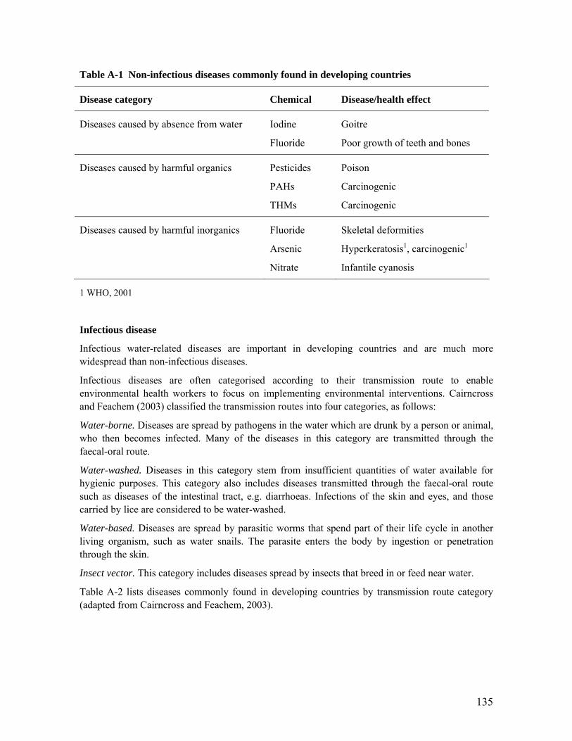
135

Table A-1 Non-infectious diseases commonly found in developing countries

Disease category Chemical Disease/health effect

Diseases caused by absence from water Iodine

Fluoride

Goitre

Poor growth of teeth and bones

Diseases caused by harmful organics Pesticides

PAHs

THMs

Poison

Carcinogenic

Carcinogenic

Diseases caused by harmful inorganics Fluoride

Arsenic

Nitrate

Skeletal deformities

Hyperkeratosis1, carcinogenic1

Infantile cyanosis

1 WHO, 2001

Infectious disease

Infectious water-related diseases are important in developing countries and are much more widespread than non-infectious diseases.

Infectious diseases are often categorised according to their transmission route to enable environmental health workers to focus on implementing environmental interventions. Cairncross and Feachem (2003) classified the transmission routes into four categories, as follows:

Water-borne. Diseases are spread by pathogens in the water which are drunk by a person or animal, who then becomes infected. Many of the diseases in this category are transmitted through the faecal-oral route.

Water-washed. Diseases in this category stem from insufficient quantities of water available for hygienic purposes. This category also includes diseases transmitted through the faecal-oral route such as diseases of the intestinal tract, e.g. diarrhoeas. Infections of the skin and eyes, and those carried by lice are considered to be water-washed.

Water-based. Diseases are spread by parasitic worms that spend part of their life cycle in another living organism, such as water snails. The parasite enters the body by ingestion or penetration through the skin.

Insect vector. This category includes diseases spread by insects that breed in or feed near water.

Table A-2 lists diseases commonly found in developing countries by transmission route category (adapted from Cairncross and Feachem, 2003).

136

Table A-1 Infectious diseases commonly found in developing countries

Transmission route Example diseases

Water-borne Cholera Typhoid Gastroenteritis Poliomyelitis Cryptosporidiosis Giardiasis Hepatitis A

Water-washed Amoebic dysentery Trachoma Scabies

Water-based Guinea worm Schistosomiasis

Insect vector Malaria Yellow Fever Dengue Fever River blindness

2. Guinea worm

Guinea worm (Dracunculus medinensis) is a preventable infection affecting communities without safe drinking water. People become infected when they ingest cyclopoids, a water flea, which carries the guinea worm larvae. The larvae then develop in the human host and fertilised female worms will move through the body of the host towards the extremities (frequently legs). The mature female worm then creates a blister on the skin, which creates a burning sensation in the host leading the host to immerse the blister in water to soothe the pain (Cairncross and Feachem, 2003). Once the blister comes into contact with water the female worm breaks through the host’s skin and deposits new larvae into the water body, which are then swallowed by the water flea and the cycle is perpetuated. The time between host infection and the appearance of a blister can take a year (Feachem and Cairncross, 2003).

Safe water provision if a key action in controlling the disease and the WHO has targeted guinea worm for eradication. The US-based organisation The Carter Center is leading an international coalition, which is working towards the eradication goal, primarily through education, monitoring and distribution of cloth filters in affected areas. Since 1986, when 3.5 million cases of guinea worm were reported across Asia and Africa, the eradication program has limited guinea worm to just over four thousand cases in five African countries in 2008 (DHHS, 2008). Sudan and Ghana have the highest proportions of cases (78% and 11% of global cases respectively), with Mali, Ethiopia and Niger all reported guinea worm cases in 2008 (DHHS, 2008). For the months January to March, 2009, Ghana has the highest recorded number of guinea worm cases for any country, with 147 confirmed cases (DHHS, 2009).

137

Many of the cloth filters distributed by The Carter Center were seen during field visits in the Tamale area by the author in January 2009.

References

Cairncross, S. and Feachem, R., 2003. Environmental Health Engineering in the Tropics An Introductory Text, John Wiley and Sons, England.

Cairncross, S. and Feachem, R., 1999. Environmental Health Engineering in the Tropics An Introductory Text, John Wiley and Sons, England.

Department of Health & Human Services (DHHS), 2009. Public Health Service, Centers for Disease Control and Prevention, Guinea worm wrap-up #189, April 20, 2008.

Department of Health & Human Services (DHHS), 2008. Public Health Service, Centers for Disease Control and Prevention, Guinea worm wrap-up #185, November 12, 2008.

World Health Organization (WHO), 2001. Arsenic in drinking water, Fact Sheet No 210, revised May 2001. http://www.who.int/mediacentre/factsheets/fs210/en/, accessed April 28, 2009.

138

APPENDIX B

Test results of International Aid biosand filters in Batamyili Village, Ghana

139

Test results for International Aid biosand filters in Batamyili village, Northern Region, Ghana

1. Overview

The following test results were performed in Batamyili village at the invitation of Issaka Balima Mussah, I-WASH District Resource Person, Savelugu/Nanton District Assembly for the E.U./UNICEF Integrated Water, Sanitation and Hygiene (I-WASH) Project. As part of this project 100 International Aid HydrAid™ plastic biosand filters were installed in Batamyili village, covering 100% of that village.

BSF samples and tests were conducted on January 23, 2009, three months after the BSFs had been installed. It was understood from Mr Mussah, and confirmed by observations on site, that the filters had been in regular use for the previous three months but there had been no prior performance or water quality testing of these BSFs. The villagers were not given prior notice of the testing so as not to influence their actions by allowing preparation for the visit which may have compromised the results (e.g. cleaning filters, temporarily using alternative source water).

A total of 25 biosand filters were sampled in 8 family compounds. Filters were filled during the tests by the usual household operator. No survey was conducted, but informal interviews with the person responsible for filter operation did take place and field notes were taken.

2. Test procedures

All tests were conducted in a manner that reduced possible contamination of samples from external sources. All BSFs were sampled for turbidity and microbiological quality after approximately 3 L of filtrate had been discharged, so that results were comparable.

Turbidity

Turbidity measurements in nephelometric turbidity units (NTU) were made using a Hach Model 2100P Portable Turbidimeter. The turbidimeter was calibrated with formazin solution and in accordance with the manufacturer’s instructions. Initial calibration was carried out upon arrival to Tamale and the turbidimeter accuracy was checked daily by reading a formazin standard (20 NTU or 100 NTU). If the turbidimeter reading of the formazin solution was more than 1 NTU off the actual value the turbidimeter was recalibrated.

The sample vial containing the water to be tested was rinsed three times with the water to be tested prior to the reading to ensure the sample was not contaminated with water previously tested. The vial was dried and wiped down with a lint free cloth prior to reading.

The turbidimeter was run in signal averaging mode as the high turbidity samples tended to give a noisy signal.

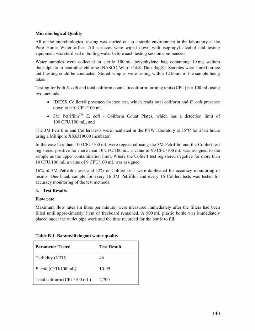
140

Microbiological Quality

All of the microbiological testing was carried out in a sterile environment in the laboratory at the Pure Home Water office. All surfaces were wiped down with isopropyl alcohol and testing equipment was sterilised in boiling water before each testing session commenced.

Water samples were collected in sterile 100 mL polyethylene bag containing 10 mg sodium thiosulphate to neutralise chlorine (NASCO Whirl-Pak® Thio-Bag®). Samples were stored on ice until testing could be conducted. Stored samples were testing within 12 hours of the sample being taken.

Testing for both E. coli and total coliform counts in coliform forming units (CFU) per 100 mL using two methods:

• IDEXX Colilert® presence/absence test, which reads total coliform and E. coli presence down to <10 CFU/100 mL.

• 3M PetrifilmTM E. coli / Coliform Count Plates, which has a detection limit of 100 CFU/100 mL, and

The 3M Petrifilm and Colilert tests were incubated in the PHW laboratory at 35°C for 24±2 hours using a Millipore XX6310000 Incubator.

In the case less than 100 CFU/100 mL were registered using the 3M Petrifilm and the Colilert test registered positive for more than 10 CFU/100 mL a value of 99 CFU/100 mL was assigned to the sample as the upper contamination limit. Where the Colilert test registered negative for more than 10 CFU/100 mL a value of 9 CFU/100 mL was assigned.

16% of 3M Petrifilm tests and 12% of Colilert tests were duplicated for accuracy monitoring of results. One blank sample for every 16 3M Petrifilm and every 16 Colilert tests was tested for accuracy monitoring of the test methods.

3. Test Results

Flow rate

Maximum flow rates (in litres per minute) were measured immediately after the filters had been filled until approximately 5 cm of freeboard remained. A 500 mL plastic bottle was immediately placed under the outlet pipe work and the time recorded for the bottle to fill.

Table B-1 Batamyili dugout water quality

Parameter Tested Test Result

Turbidity (NTU) 46

E. coli (CFU/100 mL) 10-99

Total coliform (CFU/100 mL) 2,700

141

Table B-2 Summary of biosand filter effluent quality, 25 BSFs, Batamyili village

Parameter Average reduction

Range of reduction

Influent average (standard deviation)

Filtrate average (standard deviation)

Turbidity (NTU) 78% 21% - 96% 25 (11) 5 (6)

E. coli (CFU/100 mL)1

65% 1% - >99% 399 (484) 69 (90)

Total coliform (CFU/100 mL)1

55% Increased concentration - >99% removal

10,165 (8,912) 3,340 (4,808)

1. Tests used were 3M Pertifilm and IDEXX Colilets. Where sample results indicated <100 CFU/100 mL on the 3M Petrifilms and positive for ≥10 CFU/100 mL on the Colierts an upper limit value of 99 CFU/100 mL was assigned. Where both tests were negative for colonies, an upper value of 9 CFU/100 mL was assigned.

Table B-3 Summary of biosand filter flow rates, 25 BSFs, Batamyili village

Flow rate Value

Average (L/min) 1.3

Standard deviation (L/min) 0.5

Minimum (L/min) 0.3

Maximum (L/min) 2.3

142

Table B-4 Details of biosand filter influent quality, 25 BSFs, Batamyili village

3M Petrifilm test Colilert test

Count Compound House E. coli1

(CFU/100 mL) Total coliform (CFU/100 mL) E. coli

Total coliform

Turbidity (NTU)

1 BV1 A 300 5,500 positive positive 39 2 B1 <100 2,900 positive positive 25 B2 <100 1,600 positive positive 29

3 C 300 5,500 positive positive 39 4 BV3 A 2,300 33,400 positive positive 18 5 BV4 A 1,200 25,000 positive positive 12 6 B 700 20,200 positive positive 45 7 C 700 20,200 positive positive 45 8 BV5 A 200 5,100 no data no data 21 9 B 300 9,600 positive positive 23

10 C 100 6,500 positive positive 26 11 D <100 5,000 positive positive 22 12 E 100 6,100 positive positive 12 13 F 100 6,500 positive positive 26 14 BV6 A <100 2,900 positive positive 9 15 B <100 2,600 positive positive 13 16 C <100 1,000 positive positive 7 17 BV7 A <100 1,900 positive positive 31 18 B <100 3,400 positive positive 17 19 BV8 A <100 3,400 positive positive 38 20 B <100 3,400 positive positive 38 21 BV9 A <100 18,600 positive positive 25 22 B <100 18,600 positive positive 25 23 C <100 18,600 positive positive 25 24 D <100 18,600 positive positive 25 25 E <100 18,600 positive positive 25

1 – 3M Petrifilm E. coli colonies are identified as blue colonies with gas bubbles on the incubated petrifilm. At this village, results showed 30% – 50% blue colonies without gas bubbles in addition to the count with bubbles. Petrifilms were brought back to the USA for further testing of the blue colonies without gas bubbles. However, due to the time between sampling and further testing in the USA, the blue colonies without gas died and testing was inconclusive. It could not be determined if they were also E. coli bacteria, and they have not been include in the E. coli enumeration.

143

Table B-5 Details of biosand filter effluent quality, 25 BSFs, Batamyili village

3M Petrifilm test Colilert test

Count Compound House E. coli1

(CFU/100 mL) Total coliform (CFU/100 mL) E. coli

Total coliform

Turbidity (NTU)

1 BV1 A <100 1,100 positive positive 9 2 B1 <100 2,500 positive positive 3 B2

3 C <100 <100 negative negative 6 4 BV3 A no data no data negative positive 2 5 BV4 A <100 1,000 positive positive 4 6 B 200 7,300 positive positive 4 7 C 400 8,900 positive positive 5 8 BV5 A 150 2,700 positive positive 9 9 B <100 21,500 negative positive 8

10 C <100 5,700 positive positive 4 11 D <100 2,300 positive positive 10 12 E <100 2,200 negative positive 3 13 F <100 <100 negative negative 1 14 BV6 A <100 1,900 negative positive 3 15 B <100 <100 negative negative 1 16 C <100 <100 negative negative 2 17 BV7 A <100 2,800 positive positive 3 18 B <100 7,900 positive positive 5 19 BV8 A <100 3,000 negative positive 6 20 B <100 500 negative positive 30 21 BV9 A <100 7,900 positive positive 7 22 B <100 800 negative positive 2 23 C <100 <100 negative positive 1 24 D <100 <100 negative negative 1 25 E <100 <100 negative negative 2

1 – 3M Petrifilm E. coli colonies are identified as blue colonies with gas bubbles on the incubated petrifilm. At this village, results showed 30% – 50% blue colonies without gas bubbles in addition to the count with bubbles. Petrifilms were brought back to the USA for further testing of the blue colonies without gas bubbles. However, due to the time between sampling and further testing in the USA, the blue colonies without gas died and testing was inconclusive. It could not be determined if they were also E. coli bacteria, and they have not been include in the E. coli enumeration.

144

Table B-6 Details of biosand filter performance, 25 BSFs, Batamyili village

Count Compound House BSF flow rate

(L/min) E. coli

reduction Total coliform

reduction Turbidity reduction

Covered filtrate

1 BV1 A 1.0 67% 80% 77% no 2 B 1.1 ** 14% 88% no 3 C 1.5 67% >99% 79% no 4 BV3 A 1.3 >99% N/A 89% yes 5 BV4 A 0.9 92% 96% 67% yes 6 B 1.2 71% 64% 91% no 7 C 2.0 43% 56% 89% no 8 BV5 A 1.5 25% 47% 57% no 9 B 1.4 97% increase 65% no

10 C 0.7 1% 12% 85% no 11 D 0.7 ** 54% 55% yes 12 E 0.4 91% 64% 75% yes 13 F 2.1 91% >99% 92% no 14 BV6 A 1.6 ** 34% 67% no 15 B 1.1 ** >99% 92% no 16 C 1.9 ** >99% 71% no 17 BV7 A 0.8 ** increase 90% yes 18 B 1.1 ** increase 71% yes 19 BV8 A 2.1 ** 12% 84% no 20 B 2.3 ** 85% 21% no 21 BV9 A 0.3 ** 58% 72% yes 22 B 1.2 ** 96% 92% yes 23 C 1.5 ** >99% 96% no 24 D 1.7 ** >99% 96% yes 25 E 0.9 ** >99% 92% no

** Accurate reduction could not be calculated as influent and effluent water quality data results in ranges.

145

APPENDIX C

Test results of International Aid biosand filters in Zuozugu Village, Ghana

146

Test results for International Aid biosand filters in Zuozugu Village, Northern Region, Ghana

1. Overview

The following tests were conducted for International Aid HydrAid™ biosand filters distributed in Zuozugu Village by the University of North Carolina (UNC), USA. Zuozugu village had been part of a one year study by UNC and had received the filters as part of their role as a control village. Upon completion of the study the filters remained in the village as a gift of UNC.

Tests were conducted on January 20, 2009, approximately 3 - 4 months after the filters had been installed. The villagers were not given prior notice of the testing so as not to influence their actions by allowing preparation for the visit which may have compromised the results (e.g. cleaning filters, temporarily using alternative source water).

A total of 4 biosand filters were sampled in 4 family compounds. Filters were filled during the tests by the usual household operator.

2. Test procedures

All tests were conducted in a manner that reduced possible contamination of samples from external sources. All BSFs were sampled for turbidity and microbiological quality after approximately 3 L of filtrate had been discharged, so that results were comparable.

Turbidity

Turbidity measurements in nephelometric turbidity units (NTU) were made using a Hach Model 2100P Portable Turbidimeter. The turbidimeter was calibrated with formazin solution and in accordance with the manufacturer’s instructions. Initial calibration was carried out upon arrival to Tamale and the turbidimeter accuracy was checked daily by reading a formazin standard (20 NTU or 100 NTU). If the turbidimeter reading of the formazin solution was more than 1 NTU off the actual value the turbidimeter was recalibrated.

The sample vial containing the water to be tested was rinsed three times with the water to be tested prior to the reading to ensure the sample was not contaminated with water previously tested. The vial was dried and wiped down with a lint free cloth prior to reading.

The turbidimeter was run in signal averaging mode as the high turbidity samples tended to give a noisy signal.

Microbiological Quality

All of the microbiological testing was carried out in a sterile environment in the laboratory at the Pure Home Water office. All surfaces were wiped down with isopropyl alcohol and testing equipment was sterilised in boiling water before each testing session commenced.

147

Water samples were collected in sterile 100 mL polyethylene bag containing 10 mg sodium thiosulphate to neutralise chlorine (NASCO Whirl-Pak® Thio-Bag®). Samples were stored on ice until testing could be conducted. Stored samples were testing within 12 hours of the sample being taken.

Testing for both E. coli and total coliform counts in coliform forming units (CFU) per 100 mL using two methods:

• 3M PetrifilmTM E. coli / Coliform Count Plates, which has a detection limit of 100 CFU/100 mL, and

• IDEXX Colilert® presence/absence test, which reads total coliform and E. coli presence down to <10 CFU/100 mL.

The 3M Petrifilm and Colilert tests were incubated in the PHW laboratory at 35°C for 24±2 hours using a Millipore XX6310000 Incubator.

In the case less than 100 CFU/100 mL were registered using the 3M Petrifilm and the Colilert test registered positive for more than 10 CFU/100 mL a value of 99 CFU/100 mL was assigned to the sample as the upper contamination limit. Where the Colilert test registered negative for more than 10 CFU/100 mL a value of 9 CFU/100 mL was assigned.

Duplicate and blank samples were not tested on this occasion.

3. Results

Table B-1 Zuozugu dugout water quality, 4 BSFs, Zuozugu village

Parameter Tested Test Result

Turbidity (NTU) 174

E. coli (CFU/100 mL) 10-99

Total coliform (CFU/100 mL) 2,400

148

Table B-2 Summary of biosand filter effluent quality, 4 BSFs, Zuozugu village

Parameter Average reduction

Range of reduction

Influent average (standard deviation)

Filtrate average (standard deviation)

Turbidity (NTU) 76% 52% - 90% 162 (19) 39 (37)

E. coli (CFU/100 mL)1

89% 86% - 90%2 250 (300) 32 (45)

Total coliform (CFU/100 mL)1

72% 36% - >99% 6,800 (9,905) 3,580 (6,883)

1. Tests used were 3M Petrifilm and IDEXX Colilerts. Where sample results indicated <100 CFU/100 mL on the 3M Petrifilms and positive for ≥10 CFU/100 mL on the Colilerts an upper limit value of 99 CFU/100 mL was assigned. Where both tests were negative for colonies, an upper value of 9 CFU/100 mL was assigned.

2. Based on two samples only.

Table B-3 Details of biosand filter influent quality, 4 BSFs, Zuozugu village

3M Petrifilm test Colilert test

Count Compound E. coli

(CFU/100 mL) Total coliform (CFU/100 mL) E. coli

Total coliform

Turbidity (NTU)

1 1 100 2,800 positive positive 168 2 2 700 2,100 positive positive 148 3 3 <100 700 positive positive 147 4 4 <100 21,600 positive positive 186

Table B-4 Details of biosand filter effluent quality, 4 BSFs, Zuozugu village

3M Petrifilm test Colilert test

Count Compound E. coli

(CFU/100 mL) Total coliform (CFU/100 mL) E. coli

Total coliform

Turbidity (NTU)

1 1 <100 <100 negative negative 81 2 2 <100 400 positive positive 58 3 3 <100 <100 negative negative 2 4 4 <100 13,900 negative positive 15

Table B-5 Details of biosand filter performance, 4 BSFs, Zuozugu village

Count Compound E. coli reduction Total coliform

reduction Turbidity reduction

1 1 91% >99% 52% 2 2 86% 81% 61% 3 3 ** 99% 99% 4 4 ** 36% 92%

** Accurate reduction could not be calculated as influent and effluent water quality data results in ranges.

149

APPENDIX D

Biosand filter pore volume calculations

150

Biosand filter pore volume calculations

CAWST concrete filter pore volume

Volume supernatant, Vs:

wbhVS =

where w = width (m)

b = breadth (m)

h = height (m)

VS = 0.22 m * 0.22 m * 0.05 m

VS = 0.0024 m3

VS = 2.4 L

Sand/gravel volumes required, VT:

VT = 25 L fine sand

+ 3.5 L separating gravel layer (i.e. coarse sand)

- 3 L gravel

VT = 31.5 L sand/gravel

Assuming an average sand porosity of 0.4, volume of water in the sand layers, Vw:

Tw nVV =

Vw = 0.4 * 31.5 L

Vw = 12.6 L

Total water in CAWST concrete filter, VP

VP = sum of water in sand and supernatant = VW + VS

VP = 12.6 L + 2.4 L

Vp = 15 L

All dimensions and sand/gravel volumes taken from CAWST (2008).

151

International Aid HydrAid™ filter pore volume

Weight sand and water: 60 kg (International Aid, 2009)

Volume of pore water in a cylinder, V:

zdnV4

2

π=

where n = porosity

d = diameter (m), estimated by the author based on filter dimensions given in Kikkawa (2008)

z = depth (m) of filter section

Supernatant volume:

n = 1 (water only)

V = 1 * π * (0.35 m)2/4 * 0.05 m

V = 0.005 m3 = 5 L

Superfine sand layer pore volume:

n = 0.4 (Buzunis, 1995)

V = 0.4 * π * (0.32 m)2/4 * 0.05 m

V = 0.0016 m3 = 1.6 L

Fine sand layer pore volume:

n = 0.4 (Buzunis, 1995)

V = 0.4 * π * (0.30 m)2/4 * 0.375 m

V = 0.0108 m3 = 10.8 L

Coarse sand layer pore volume:

n = 0.3 (EPA, 1998)

V = 0.3 * π * (0.27 m)2/4 * 0.051 m

V = 0.0009 m3 = 0.9 L

Gravel layer pore volume:

n = 0.3 (EPA, 1998)

V = 0.3 * π * (0.26 m)2/4 * 0.057 m

V = 0.0009 m3 = 0.9 L

Water in the drainage pipe:

n = 1 (water only)

¼ inch pipe = 0.008 m diameter

Drainage pipe length = 0.2 m

152

Vertical pipe length = 0.5 m

Total pipe length = 0.7 m

V = 1 * π * (0.008 m)2/4 * 0.7 m

V = 0.0004 m3 = 0.4 L

Total water in International Aid HydrAid™ BSF, pore volume Vp

total Vp = sum of pore volumes

Vp = 19.6 L ≈ 20 L

References

Buzunis, B.J., 1995. Intermittently Operated Slow Sand Filtration: A New Water Treatment Process, University of Calgary Master of Engineering Thesis, Calgary, AL, Canada.

Centre for Affordable Water and Sanitation Technology (CAWST), 2008. Biosand Filter Manual, Calgary, Canada.

International Aid, 2009. HydrAid™ Biosand Water Filter, http://www.hydraid.org/, accessed May 7, 2009.

Kikkawa, I., 2008. Modification of the Biosand Filter in the Northern Region of Ghana, Massachusetts Institute of Technology Master of Engineering Thesis, Cambridge, MA, USA.

United States Environmental Protection Agency (US EPA), 1998. Technical Protocol for Evaluating Natural Attenuation of Chlorinated Solvents in Ground Water, EP/600/R-98/128, September 1998.

153

APPENDIX E

Dissolved oxygen solubility in water as a function of temperature

154

Dissolved oxygen solubility in water as a function of temperature Concentrations sourced from a table of values attached to the YSI Model 57 Oxygen Meter used for the dissolved oxygen concentration readings taken as part of this thesis research. Concentrations are given for 1 atm pressure.

Temperature (°C)

Dissolved oxygen (mg/L)

Temperature (°C)

Dissolved oxygen (mg/L)

0 14.62 24 8.42 1 14.22 25 8.26 2 13.83 26 8.11 3 13.46 27 7.97 4 13.11 28 7.83 5 12.77 29 7.69 6 12.45 30 7.56 7 12.14 31 7.43 8 11.84 32 7.31 9 11.56 33 7.18

10 11.29 34 7.07 11 11.03 35 6.95 12 10.78 36 6.84 13 10.54 37 6.73 14 10.31 38 6.62 15 10.08 39 6.52 16 9.87 40 6.41 17 9.67 41 6.31 18 9.47 42 6.21 19 9.28 43 6.12 20 9.09 44 6.02 21 8.92 45 5.93 22 8.74 46 5.84 23 8.58 47 5.74