BIOS 312: MODERN REGRESSION...

BIOS 312: MODERN REGRESSION ANALYSIS

James C (Chris) SlaughterDepartment of Biostatistics

Vanderbilt University School of [email protected]

biostat.mc.vanderbilt.edu/CourseBios312

Copyright 2009-2012 JC Slaughter All Rights ReservedUpdated March 26, 2012

Contents

14 Regression Based Prediction 5

14.1 Overview . . . . . . . . . . . . . . . . . . . . . . . . . . . . . . . . 5

14.1.1 Uses of Regression . . . . . . . . . . . . . . . . . . . . . . 5

14.1.2 Examples of Prediction . . . . . . . . . . . . . . . . . . . . 7

14.1.3 Assumptions needed for inference . . . . . . . . . . . . . . 10

14.2 Estimation (prediction) of summary measures . . . . . . . . . . . . 11

14.2.1 Point estimates . . . . . . . . . . . . . . . . . . . . . . . . . 12

14.2.2 Interval estimates . . . . . . . . . . . . . . . . . . . . . . . 12

14.3 Prediction (forecasting) of individual observations . . . . . . . . . . 17

14.3.1 Assumptions . . . . . . . . . . . . . . . . . . . . . . . . . . 17

14.3.2 Point and interval estimates for Normal data . . . . . . . . . 19

14.3.3 Example: FEV by age and height . . . . . . . . . . . . . . . 21

14.3.4 Mathematics of Prediction Intervals . . . . . . . . . . . . . 23

14.4 Prediction of Binary Measurements . . . . . . . . . . . . . . . . . . 23

14.4.1 Classification (discrimination) . . . . . . . . . . . . . . . . . 23

3

CONTENTS 4

14.4.2 Stepwise model building . . . . . . . . . . . . . . . . . . . . 25

14.4.3 ROC Curves . . . . . . . . . . . . . . . . . . . . . . . . . . 26

14.4.4 Example 1: Age or height to predict smoking . . . . . . . . 27

14.4.5 Example 2: Multiple predictors of smoking . . . . . . . . . . 30

14.4.6 Analysis of ROC curves in R . . . . . . . . . . . . . . . . . 34

14.4.7 Multivariable prognostic models . . . . . . . . . . . . . . . . 34

Chapter 14

Regression Based Prediction

14.1 Overview

14.1.1 Uses of Regression

· Cluster Analysis

– Focuses on identifying observations (covariates) with similar characteris-tics∗ Interest lies in finding clusters that are more (or less) likely to have

some outcome of interest

– Divide a population into subgroups based on patterns of similar measure-ment∗ Clustering can be done by considering one variable (univariable) or

multiple variables (multivariable)

∗ Number of clusters can be known or unknown

– Examples∗ Microarrays

5

CHAPTER 14. REGRESSION BASED PREDICTION 6

∗ fMRI

∗ “Small n, large p” (few subjects, many predictors)

– Statistical techniques∗ Stepwise regression

∗ Regression trees

∗ Other data-driven model building approaches

∗ Getting valid inference (i.e. reliable p-values, unbiased parameter es-timates) particularly challenging· Area of active research in Biostatistics

· Quantifying and comparing distributions

– Compare distribution of the outcome variable across levels of the group-ing variable or variables∗ Compare salary in males and females, across professors of the same

rank, degree, experience, and field

∗ Compare FEV in smokers and non-smokers, across teenagers of thesame age and height

– Need to decide which summary measure is appropriate for describingthe distribution∗ Common summary measures: Means, median, geometric mean, odds,

rates, hazards

∗ Other measures: Variance, skewness, kurtosis, likelihood of extremevalues, quantiles, etc.


– May desire estimates within specific subgroups∗ Estimates of the association within gender, race, or age groups

∗ (This is effect modification)

· Regression based prediction

– Prediction of summary measures∗ Point prediction· Best single estimate for the measurement that would be obtained,

on average, for many individuals with given covariates

∗ Interval prediction· Quantify the uncertainty of the average

· Range of summary measure that might be reasonable to observe

– Prediction of individual measurements∗ Point prediction· Best single estimate for the measurement that would be obtained

on a single individual with given covariates

∗ Interval prediction· Quantify the uncertainty of the individual prediction

· Range of measurements that might reasonably be observed in afuture individual with given covariates

14.1.2 Examples of Prediction

Continuous prediction: Creatinine clearance

· Creatinine is a continuously produced breakdown product in muscles


· Removed by the kidney through filtration

· Amount of creatinine cleared by the kidneys in 24 hours is a measure ofrenal function

– Gold standard is to collect urine output for 24 hours, measure creatinine

– Would prefer to find a combination of blood and urine measures that canbe obtained at one time point, yet still provides accurate prediction of apatient’s creatinine clearance

· Statistical approach

– Collect a training dataset to build a regression model for prediction∗ Measure true creatinine clearance

∗ Measure age, gender, weight, height, blood makers, urinary markers,etc.

∗ Fit a (data driven?) regression model to predict true creatinine clear-ance

– Collect a validation dataset∗ Use the regression estimates (the βs) from the training dataset to see

how well your model predict creatinine clearance

∗ Quantify the accuracy of the predictive model (e.g. mean squarederror)

∗ Cross validation


Discrimination (binary prediction): Low birth weight

· Want to predict which infants are more likely to be less than 2500 grams atbirth

· Possible predictors: Age, race, blood biomarkers collected during pregnancy

· Statistical Approach

– Collect a training dataset to build a regression model for prediction∗ Measure birth weight

∗ Measure age, race, blood biomarkers

∗ Fit a (data driven?) regression model to predict low birth weight

– Collect a validation dataset∗ Use the regression estimates (the βs) from the training dataset to see

how well your model predict low birth weight

∗ Quantify the accuracy of the predictive model· Sensitivity, specificity (ROC curves)

· Predictive value positive, predictive value negative

Interval prediction: Normal ranges of PSA

· Identify the range of PSA values that would be expected in 95% of mosthealthy adult males

· Possibly stratify by age, race

· Statistical Approach


– Collect a training dataset to build a regression model for prediction∗ Measure PSA and variable to predict PSA

∗ Need to estimate the quantiles· Mean plus/minus 2 standard deviations (makes strong Normality

assumption)

· Estimate the quantiles, provide CIs around the quantiles (likely lowprecision)

– Collect a validation dataset∗ Quantify the accuracy of the predictive model (e.g. coverage proba-

bilities)

14.1.3 Assumptions needed for inference

Inference for associations

· Necessary assumptions for classical regression (no robust standard errors)

– Independence of response measurements within identified clusters

– Have appropriately modeled the within group variance∗ Linear regression: Equal variance across groups

∗ Other regressions: Appropriate mean-variance relationship· Lack of model fit may lead to poor estimate of the variance

– Sample size is large enough so that parameter estimates approximatelyfollow a Normal distribution

· Necessary assumptions for first order trends using robust standard errors

– Independence of response measurements within identified clusters


– (Robust standard errors accounts for heteroscedasticity in large sam-ples)∗ Lack of model fit leads to conservative inference due to mixing sys-

tematic and random error

– Sample size is large enough so that parameter estimates approximatelyfollow a Normal distribution

Inference for predictions

· Additional assumptions for predictions of means

– Our regression model has accurately described the relationship betweensummary measures across groups

– For continuous covariates, often involves flexible models that allow fordepartures from linearity

· Additional assumptions for predictions of individual observations

– Also need to know the shape of the distribution within each group

– Methods implemented in software often rely on strong assumptions likeNormality

14.2 Estimation (prediction) of summary measures

· Given age, height, and sex, estimate the mean (or geometric mean) FEV

– Use linear regression to obtain estimates and CI

· Given age and PSA, estimate the probability (or odds) of remaining in remis-sion for 24 months


– Use logistic regression to obtain estimates and CI

· Assumptions

– Independence (between clusters for robust SE)

– Variance approximated by the model (relaxed for robust SE)

– Regression model accurately describes the relationship of summary mea-sures across groups

– Sufficient sample sizes for asymptotic distributions of parameters to be agood approximation

14.2.1 Point estimates

· Point estimates obtained by substitution of predictor values into the esti-mated regression equation

– E[Chol|Age] = 200 + 0.33× Age

∗ Expected cholesterol for 50 year old is 200 + 0.33× 50 = 216.5

– logodds(Survival|Age) = −0.1365− 0.007899× Age

∗ Expected log-odds of Survival for a 50 year old is −0.1365−0.007899×50 = −0.53

∗ Expected odds = e−.53 = 0.59

∗ Expected probability = 0.37

14.2.2 Interval estimates

· If assumptions hold, interval estimates can be obtained


– We generally find a confidence interval for the transformed quantity, andthen back transform to the desired quantity∗ For logistic regression, calculate the CI for the log odds, the transform

to odds or probability

· Statistical criteria for determining the “best” estimate

– Consistent: Correct estimate (with infinite sample size)

– Precise: Minimum variance among (unbiased) estimators

– Common regression methods provide the best estimate in a wide varietyof settings

· Necessary assumptions

– Independence

– Variance approximated by the model (relaxed for robust SE)

– Regression model accurately describes the relationship among sum-mary measures across groups

– Sufficient sample size so that asymptotic Normality of the parameter es-timates holds

· Interval estimates

– When we substitute in the predictor values, it provides an estimate of themodel transformation of the summary measure

– Model transformation of the summary measure varies by regression set-ting∗ Linear regression: Mean


∗ Linear regression on log transformed outcome: Log geometric mean

∗ Logistic regression: Log odds

∗ Poisson regression: Log rate

– Formulas for the confidence interval∗ In general: (estimate)± (crit value)× (std error)

∗ In linear regression, the t distribution is usually used to obtain theconfidence interval· Stata: (crit value) = invttail(df, α/2)

· R: (crit value) = qt(1− α/2, df)

· Degrees of freedom df = n− number of predictors in model

∗ In other regressions, we use the standard Normal distribution· Stata: (crit value) = invnorm(1− α/2) = 1.96

· R: (crit value) = qnorm(1− α/2) = 1.96

· Interval estimates in Stata

– After any regression command, the Stata command predict will givecompute estimates and standard errors

– predict varname, [what]

∗ varname is that name of the new variable to be created

∗ what is one of· xb: The linear predictor (works for all regression)


· stdp: Standard error of the linear prediction

· p: For logistic regression, to predicted probability

· Interval estimates in R

– After storing a model, the R function predict will give compute estimatesand standard errors

– predict(object, se.fit=FALSE, ...)

∗ object is the stored fitted model

∗ se.fit will provide the standard error of the fit (defaults to FALSE)

∗ See help(predict) for more details and options


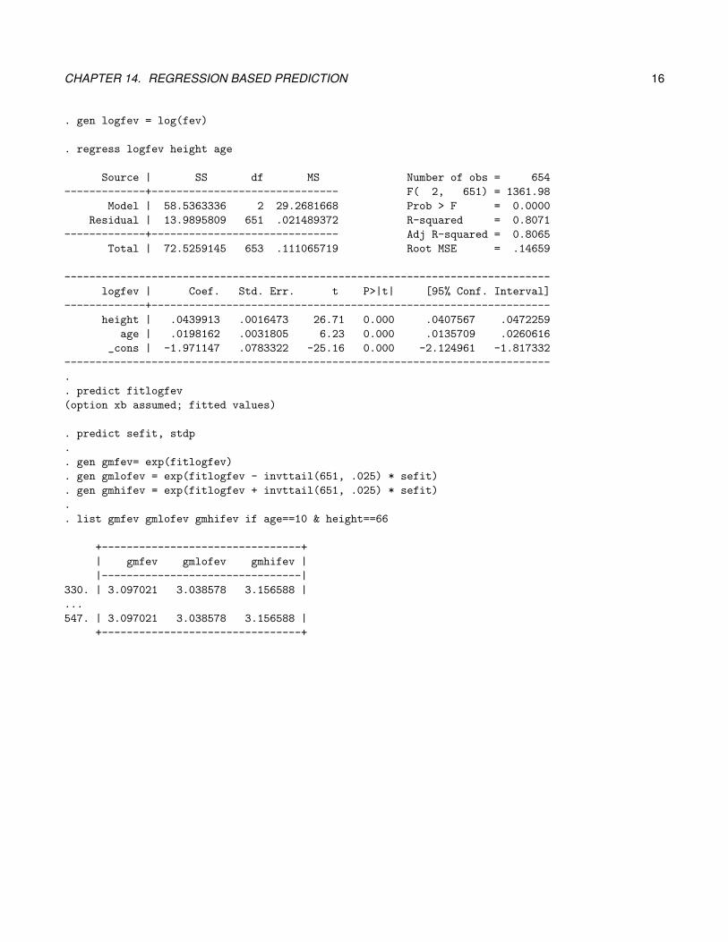
. gen logfev = log(fev)

. regress logfev height age

Source | SS df MS Number of obs = 654

-------------+------------------------------ F( 2, 651) = 1361.98

Model | 58.5363336 2 29.2681668 Prob > F = 0.0000

Residual | 13.9895809 651 .021489372 R-squared = 0.8071

-------------+------------------------------ Adj R-squared = 0.8065

Total | 72.5259145 653 .111065719 Root MSE = .14659

------------------------------------------------------------------------------

logfev | Coef. Std. Err. t P>|t| [95% Conf. Interval]

-------------+----------------------------------------------------------------

height | .0439913 .0016473 26.71 0.000 .0407567 .0472259

age | .0198162 .0031805 6.23 0.000 .0135709 .0260616

_cons | -1.971147 .0783322 -25.16 0.000 -2.124961 -1.817332

------------------------------------------------------------------------------

.

. predict fitlogfev

(option xb assumed; fitted values)

. predict sefit, stdp

.

. gen gmfev= exp(fitlogfev)

. gen gmlofev = exp(fitlogfev - invttail(651, .025) * sefit)

. gen gmhifev = exp(fitlogfev + invttail(651, .025) * sefit)

.

. list gmfev gmlofev gmhifev if age==10 & height==66

+--------------------------------+

| gmfev gmlofev gmhifev |

|--------------------------------|

330. | 3.097021 3.038578 3.156588 |

...

547. | 3.097021 3.038578 3.156588 |

+--------------------------------+


. logit smoker height age

Logistic regression Number of obs = 654

LR chi2(2) = 106.39

Prob > chi2 = 0.0000

Log likelihood = -158.52851 Pseudo R2 = 0.2512

------------------------------------------------------------------------------

smoker | Coef. Std. Err. z P>|z| [95% Conf. Interval]

-------------+----------------------------------------------------------------

height | .0505297 .0410562 1.23 0.218 -.029939 .1309984

age | .4377213 .0661923 6.61 0.000 .3079868 .5674557

_cons | -10.45429 2.351283 -4.45 0.000 -15.06272 -5.845856

------------------------------------------------------------------------------

. predict logodds, xb

. predict selogodds, stdp

.

. gen odds= exp(logodds)

. gen oddslo= exp(logodds - 1.96 * selogodds)

. gen oddshi= exp(logodds + 1.96 * selogodds)

. list odds oddslo oddshi if age==10 & height==66

+--------------------------------+

| odds oddslo oddshi |

|--------------------------------|

330. | .0644342 .0400909 .1035588 |

...

547. | .0644342 .0400909 .1035588 |

+--------------------------------+

14.3 Prediction (forecasting) of individual observations

· Methods are for continuous outcomes

– Will deal with discrimination of binary outcomes in next section

· Given age, height, and sex, predict a new subject’s FEV

– Use linear regression to obtain estimates and CI

14.3.1 Assumptions

· Necessary assumptions to predict individual observations


– Independence (between clusters for robust SE)

– Variance approximated by the model (NOT relaxed for robust SE)

– Regression model accurately describes the relationship of summary mea-sures across groups

– Shape of the distribution the same in each group∗ Transformation of the outcome may be very useful

– Sufficient sample sizes for asymptotic distributions of parameters to be agood approximation

· Assumptions are very strong

– Consequently, we do not have many methods that provide robust infer-ence∗ In general, I prefer methods that make as few assumptions as possible

∗ Robust standard errors will not help in this situation

– Proper transformation of outcomes and predictors may be necessary sothat underlying assumptions of classical linear regression model hold∗ Models, estimates, will need to be appropriately penalized for valid

inference

∗ Topic of more advanced regression courses (Regression ModelingStrategies)

– Precise methods have been developed for∗ Binary variables (the mean specifies the variances)

∗ Continuous data that follow a Normal distribution


14.3.2 Point and interval estimates for Normal data

· Point estimates obtained by substitution into the estimated regression equa-tion

– E[Chol|Age] = 200 + 0.33× Age

∗ Expected cholesterol for 50 year old is 200 + 0.33× 50 = 216.5

– When we substitute in age values, it provides an estimate of the forecastcholesterol

· Interval estimates

– Under appropriate assumptions, we can obtain standard errors for suchpredictions

– Standard errors must account for two sources of variability∗ Variability in estimating the regression parameters (same as in predic-

tions of summary measures)

∗ Variability due to subject· Additional variability about the sample mean; “within group stan-

dard deviation”

· Estimating this sources of variability is where the additional Nor-mality assumption is key

– Formulas for the prediction interval∗ In general: (prediction)± (crit value)× (std error)

∗ In linear regression, the t distribution is usually used to obtain theprediction interval· Stata: (crit value) = invttail(df, α/2)

· R: (crit value) = qt(1− α/2, df)


· Degrees of freedom df = n− number of predictors in model

· Interval estimates in Stata

– After any regression command, the Stata command predict will givecompute estimates and standard errors

– predict varname, [what]

∗ varname is that name of the new variable to be created

∗ what is one of· xb: The linear predictor (works for all regression)

· stdf: Standard error of the forecast prediction

· Interval estimates in R

– After storing a model, the R function predict will give compute estimatesand standard errors

– predict(object, se.fit=FALSE, ...)

∗ object is the stored fitted model

∗ se.fit will provide the standard error of the fit (defaults to FALSE)

∗ For the standard error of the forecast, need to include the root meansquared error· se2pred = se2fit + RMSE2

· General comment about software

– Commercial software only implements prediction intervals by assumingNormal data


– If using R libraries (or Stata ado files) for prediction, carefully investigateand understand how they are making predictions∗ Don’t trust the “black box” to be giving you results that are widely ap-

plicable to all situations

– Be careful that you understand exactly what is going on if you are inter-ested in making predictions

14.3.3 Example: FEV by age and height

. regress logfev height age

Source | SS df MS Number of obs = 654

-------------+------------------------------ F( 2, 651) = 1361.98

Model | 58.5363336 2 29.2681668 Prob > F = 0.0000

Residual | 13.9895809 651 .021489372 R-squared = 0.8071

-------------+------------------------------ Adj R-squared = 0.8065

Total | 72.5259145 653 .111065719 Root MSE = .14659

------------------------------------------------------------------------------

logfev | Coef. Std. Err. t P>|t| [95% Conf. Interval]

-------------+----------------------------------------------------------------

height | .0439913 .0016473 26.71 0.000 .0407567 .0472259

age | .0198162 .0031805 6.23 0.000 .0135709 .0260616

_cons | -1.971147 .0783322 -25.16 0.000 -2.124961 -1.817332

------------------------------------------------------------------------------

. predict fitlogfev

(option xb assumed; fitted values)

. predict sepredict, stdf

. gen predfev= exp(fitlogfev)

. gen predlofev = exp(fitlogfev - invttail(651, .025) * sepredict)

. gen predhifev = exp(fitlogfev + invttail(651, .025) * sepredict)

. list predfev predlofev predhifev if age==10 & height==66

+--------------------------------+

| predfev predlo~v predhi~v |

|--------------------------------|

330. | 3.097021 2.320911 4.132662 |

...

547. | 3.097021 2.320911 4.132662 |

+--------------------------------+

· The preceding output gave prediction for individual observations


· We can compare these results to the prediction for summary measures donepreviously (see below)

+-----------------------------------------------------------------+

| gmfev gmlofev gmhifev predfev pre~ofev predhi~v |

|-----------------------------------------------------------------|

330. | 3.097021 3.038578 3.156588 3.097021 2.320911 4.132662 |

+-----------------------------------------------------------------+

– Point estimates identical

– Confidence interval for individual predictions is wider

– As n increases, the width of the prediction interval (on the log scale)approaches ±1.96× RMSE

– As n increases, the width of the interval around the summary measureapproaches 0

· We can also calculate the standard error of the prediction

· Example: Age is 10 and Height is 66. gen sepredict2 = sepredict^2

. gen sefit2 = sefit^2

. list sepredict sefit sepredict2 sefit2 if age==10 & heigh==66

+------------------------------------------+

| sepred~t sefit sepred~2 sefit2 |

|------------------------------------------|

330. | .1469132 .009702 .0215835 .0000941 |

+------------------------------------------+

. di .14659^2 +.0000941

.02158273

– se2pred = se2fit + RMSE2

∗ sepred = 0.1469132

∗ sefit = 0.0215835

∗ RMSE = 0.14659


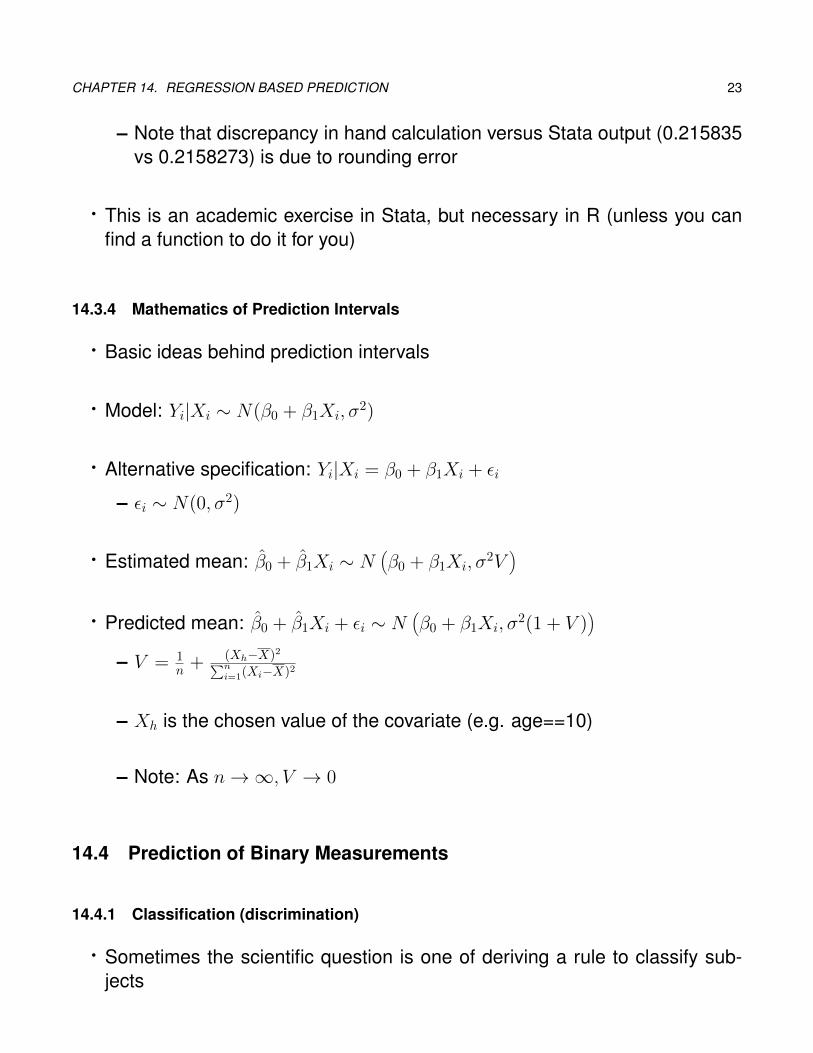
– Note that discrepancy in hand calculation versus Stata output (0.215835vs 0.2158273) is due to rounding error

· This is an academic exercise in Stata, but necessary in R (unless you canfind a function to do it for you)

14.3.4 Mathematics of Prediction Intervals

· Basic ideas behind prediction intervals

· Model: Yi|Xi ∼ N(β0 + β1Xi, σ2)

· Alternative specification: Yi|Xi = β0 + β1Xi + εi

– εi ∼ N(0, σ2)

· Estimated mean: β̂0 + β̂1Xi ∼ N(β0 + β1Xi, σ

2V)

· Predicted mean: β̂0 + β̂1Xi + εi ∼ N(β0 + β1Xi, σ

2(1 + V ))

– V = 1n + (Xh−X)2∑n

i=1(Xi−X)2

– Xh is the chosen value of the covariate (e.g. age==10)

– Note: As n→∞, V → 0

14.4 Prediction of Binary Measurements

14.4.1 Classification (discrimination)

· Sometimes the scientific question is one of deriving a rule to classify sub-jects


– Diagnosis of prostate cancer: Based on age, race, and PSA, should wemake a diagnosis of prostate cancer?

– Prognosis of patients with primary biliary cirrhosis: Based on age, biliru-bin, albumin, edema, protime, is the patient likely to die within the nextyear?

· Classification can be regarded as trying to predict the value of a binary vari-able

– Earlier, we were estimating the probability and odds of relapse within aparticular group (a summary measure)

– Now we want to decide whether a particular individual will relapse or not(an individual measure)

– There is an obvious connection between the above two ideas∗ The probability or odds tells us everything about the distribution of

values

∗ The only possible values are 0 or 1

· Typical approach

– First, use regression model to estimate the probability of event in eachgroup

– Second, form a decision rule based on estimated probability of event∗ If estimate ≥ c (or ≤ c), predict outcome is 1

∗ If estimate < c (or > c), predict outcome is 0

– Quantify the accuracy of the decision rule


– For disease D and test T∗ Sensitivity: Pr(T+|D+)

∗ Specificity: Pr(T−|D−)

∗ Predicted Value Positive: Pr(D+|T+)

∗ Predicted Value Negative: Pr(D−|T−)

14.4.2 Stepwise model building

· Old method for considering a large number of covariates that might possiblybe predictive of an outcome

– “If stepwise model building had been proposed today, it would not havepassed peer review”

· Available in all software as an automated tool, but should not be used

· Avoid recreating the stepwise approach when building your own modelsmanually

· Major caveats

– Overfits your dataset

– P-values are not true p-values; they are very anti-conservative

– You will often obtain different models if you use “forward” or “backward”stepwise regression

– Ignores confounding effects (a variable could be an important confounder,but itself not be statistically significant in the model)


– Without clustering certain predictors, may throw out covariates to makenon-sensical model∗ Suppose race/ethnicity is coded as White, Black, Hispanic, Other

∗ Want to model as 3 dummy variables

∗ Stepwise may throw out one of your dummy variables, keep the rest

∗ Pairwise significance would also be highly dependent on referencegroup chosen by analyst

· Two flavors of stepwide model building

– Start with no covariates: “Forward” stepwise regression

– Start with all covariates: “Backward” stepwise regression

· Stepwise procedure proceeds by adding or removing covariates from themodel base on the corresponding partial t or Z test

– Must pre-specify a “P to enter” and “P to remove”

– To avoid infinite loops, P to enter must be less than P to remove

– E.g. Add a variable to the model if p < 0.05, but only remove a variablefrom the model if p > 0.10

– Repeat the process until you arrive at a final model

14.4.3 ROC Curves

· Receiver operating characteristic (ROC) curves plot the sensitivity againstthe false positive rate (e.g. 1 - specificity)


· Ideal tests will have both high sensitivity and high specificity (low false posi-tives)

– Graphically depicted as points in the upper left portion of the plot

– 1:1 line represents a test that is no better than the flip of a coin

· Test usually involves the classification of some binary outcome by a contin-uous predictor (or set of continuous predictors)

– When the continuous predictor is above some point c, the test is said tobe positive

– ROC curves plots the sensitivity and false positive rate for all possiblevalues of c

· Major drawbacks to ROC analysis

– Tempts analyst to find a cutoff point (c) when none really exists

– Better to treat your covariate or linear prediction as a continuous variable

14.4.4 Example 1: Age or height to predict smoking

· Question: Is age or height a better predictor of smoking status?

· Will compare the ROC curves

– Often done use the area under the curve (AUC)

– Model with higher AUC is better

– A null model (not predictive of outcome) will have area of 0.50

– Maximum AUC is 1.0


· Stata

– Fit the logistic regression model

– lroc creates the ROC curve

– predict to save the fitted curves

– roccomp to compare the curves


. logit smoker height


LR chi2(1) = 58.27

Prob > chi2 = 0.0000


------------------------------------------------------------------------------


-------------+----------------------------------------------------------------

height | .2067181 .0307986 6.71 0.000 .1463539 .2670824

_cons | -15.32622 2.017127 -7.60 0.000 -19.27972 -11.37273

------------------------------------------------------------------------------

. lroc, nograph

Logistic model for smoker

number of observations = 654

area under ROC curve = 0.7882

. predict xb1, xb

.

. logit smoker age


LR chi2(1) = 104.88

Prob > chi2 = 0.0000


------------------------------------------------------------------------------


-------------+----------------------------------------------------------------

age | .4836394 .0551278 8.77 0.000 .375591 .5916878

_cons | -7.743905 .7089008 -10.92 0.000 -9.133325 -6.354485

------------------------------------------------------------------------------

. lroc, nograph

Logistic model for smoker

number of observations = 654

area under ROC curve = 0.8677

. predict xb2, xb

. roccomp smoker xb1 xb2, graph summary

ROC -Asymptotic Normal--

Obs Area Std. Err. [95% Conf. Interval]

-------------------------------------------------------------------------

xb1 654 0.7882 0.0225 0.74414 0.83227

xb2 654 0.8677 0.0185 0.83152 0.90393

-------------------------------------------------------------------------

Ho: area(xb1) = area(xb2)

chi2(1) = 11.20 Prob>chi2 = 0.0008


· Age has a significantly larger AUC than Height (p < 0.001)

· For any given false positive rate, the sensitivity is higher for age

– Predicted value positive would also always be higher

14.4.5 Example 2: Multiple predictors of smoking

· Will consider age, height, sex, and fev as predictors of smoking

· Fit a multivariable logistic regression model using these covariates in a train-ing sample

– Training sample will contain 60% of the observation in the current study

– Develop a model on the training sample, see how well it fits in the valida-tion sample (the remaining 40% of the data)


· Consider a rule that predicts a subject will smoke if their predicted probabilityis greater than 0.5

– Could choose other cutoffs than 0.5

– Other cutoffs will be represented on the ROC curves

– Sensitivity, specificity will vary by the cutoff chosen


.

. xi: logit smoker age height i.sex fev if training < .6

i.sex _Isex_1-2 (_Isex_1 for sex==female omitted)


LR chi2(4) = 80.02

Prob > chi2 = 0.0000


------------------------------------------------------------------------------


-------------+----------------------------------------------------------------

age | .6611145 .1276124 5.18 0.000 .4109988 .9112302

height | .1834778 .0960597 1.91 0.056 -.0047957 .3717514

_Isex_2 | -.7128769 .5392144 -1.32 0.186 -1.769718 .3439639

fev | -1.123659 .4514655 -2.49 0.013 -2.008515 -.2388024

_cons | -18.18847 5.100367 -3.57 0.000 -28.18501 -8.191936

------------------------------------------------------------------------------

. predict pfit

(option pr assumed; Pr(smoker))

.

. gen pfit50=pfit

. recode pfit50 0/0.5=0 0.5/1=1

(pfit50: 654 changes made)

.

. tabulate smoker pfit50 if training > .6, row col

| pfit50

smoker | 0 1 | Total

-----------+----------------------+----------

0 | 226 10 | 236

| 95.76 4.24 | 100.00

| 90.04 55.56 | 87.73

-----------+----------------------+----------

1 | 25 8 | 33

| 75.76 24.24 | 100.00

| 9.96 44.44 | 12.27

-----------+----------------------+----------

Total | 251 18 | 269

| 93.31 6.69 | 100.00

| 100.00 100.00 | 100.00

· Using a cutoff of 0.50

– Sensitivity: 8/33 = 24.24

– Specificity: 226/236 = 95.76


– PVP: 8/18 = 44.44

– PVN: 226/251 = 90.04

· Thresholds other than 0.50 give different values for sensitivity, specificity,PVP, PVN

– ROC curve displayed gives all possible thresholds


14.4.6 Analysis of ROC curves in R

· There are a number of add on packages that will conduct ROC analysis in R

· ROCR is one popular package

14.4.7 Multivariable prognostic models

· Reference

– Harrell FE Jr, Lee KL, Mark DB. Multivariable prognostic models: issuesin developing models, evaluating assumptions and adequacy, and mea-suring and reducing errors. Statistics in Medicine. 15(4): 361-87, Feb1996

– A “Tutorial is Biostatistics” (frequently appears in Statistics in Medicine)


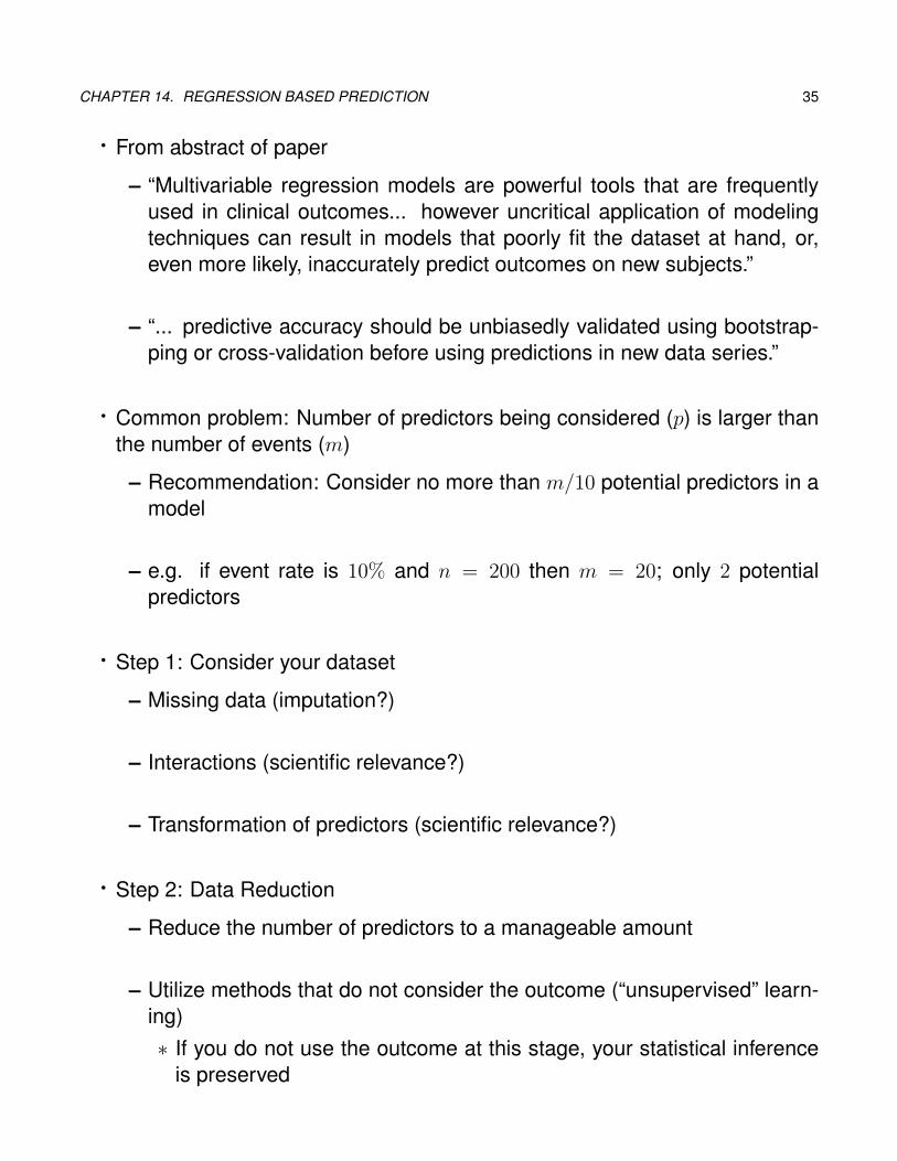
· From abstract of paper

– “Multivariable regression models are powerful tools that are frequentlyused in clinical outcomes... however uncritical application of modelingtechniques can result in models that poorly fit the dataset at hand, or,even more likely, inaccurately predict outcomes on new subjects.”

– “... predictive accuracy should be unbiasedly validated using bootstrap-ping or cross-validation before using predictions in new data series.”

· Common problem: Number of predictors being considered (p) is larger thanthe number of events (m)

– Recommendation: Consider no more than m/10 potential predictors in amodel

– e.g. if event rate is 10% and n = 200 then m = 20; only 2 potentialpredictors

· Step 1: Consider your dataset

– Missing data (imputation?)

– Interactions (scientific relevance?)

– Transformation of predictors (scientific relevance?)

· Step 2: Data Reduction

– Reduce the number of predictors to a manageable amount

– Utilize methods that do not consider the outcome (“unsupervised” learn-ing)∗ If you do not use the outcome at this stage, your statistical inference

is preserved


∗ Correlations among predictors: Variable clustering, principle compo-nents analysis

∗ Scientifically meaningful summary measures

· Step 3: Fit the model and ...

– Evaluate modeling assumptions: Linearity, additivity, distributional as-sumptions

– Use backwards stepwise selection to find a simpler model∗ Harrell: Remove predictor if χ2 > 2 (p > 0.16)

– Will use all data to fit model

· Step 4: Evaluate model

– Bootstrap cross-validation∗ Sample data with replacement

∗ For each bootstrap sample, the evaluation of modeling assumptionsand backwards selection will be performed (these steps use the out-come)

∗ Summarize predictive accuracy using a statistic (C-index, Brier score)

– Bootstrap cross-validation provides a nearly unbiased estimate of predic-tive accuracy (e.g. C-index, Brier score) while allowing the entire modelto be used for model development∗ C-index: Area under the ROC curve. Index near 1 indicates higher

accuracy.

∗ Brier score: Average squared deviation between predicted probabil-ity of event and observed outcome. A lower score represents higher


accuracy.

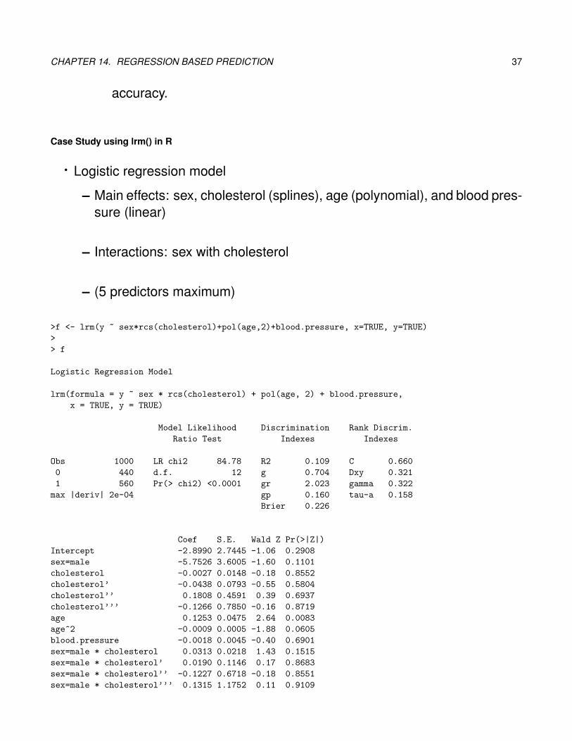
Case Study using lrm() in R

· Logistic regression model

– Main effects: sex, cholesterol (splines), age (polynomial), and blood pres-sure (linear)

– Interactions: sex with cholesterol

– (5 predictors maximum)

>f <- lrm(y ~ sex*rcs(cholesterol)+pol(age,2)+blood.pressure, x=TRUE, y=TRUE)

>

> f

Logistic Regression Model

lrm(formula = y ~ sex * rcs(cholesterol) + pol(age, 2) + blood.pressure,

x = TRUE, y = TRUE)

Model Likelihood Discrimination Rank Discrim.

Ratio Test Indexes Indexes

Obs 1000 LR chi2 84.78 R2 0.109 C 0.660

0 440 d.f. 12 g 0.704 Dxy 0.321

1 560 Pr(> chi2) <0.0001 gr 2.023 gamma 0.322

max |deriv| 2e-04 gp 0.160 tau-a 0.158

Brier 0.226

Coef S.E. Wald Z Pr(>|Z|)

Intercept -2.8990 2.7445 -1.06 0.2908

sex=male -5.7526 3.6005 -1.60 0.1101

cholesterol -0.0027 0.0148 -0.18 0.8552

cholesterol’ -0.0438 0.0793 -0.55 0.5804

cholesterol’’ 0.1808 0.4591 0.39 0.6937

cholesterol’’’ -0.1266 0.7850 -0.16 0.8719

age 0.1253 0.0475 2.64 0.0083

age^2 -0.0009 0.0005 -1.88 0.0605

blood.pressure -0.0018 0.0045 -0.40 0.6901

sex=male * cholesterol 0.0313 0.0218 1.43 0.1515

sex=male * cholesterol’ 0.0190 0.1146 0.17 0.8683

sex=male * cholesterol’’ -0.1227 0.6718 -0.18 0.8551

sex=male * cholesterol’’’ 0.1315 1.1752 0.11 0.9109


· Validation...

– Backwards stepwise regression∗ Different bootstrap sample will remove different covariates

∗ Indicates which covariates were included for each sample

– Estimates of discrimination indexes

> validate(f, B=150, bw=TRUE, rule="p", sls=.1, type="individual")

Backwards Step-down - Original Model

Deleted Chi-Sq d.f. P Residual d.f. P AIC

blood.pressure 0.16 1 0.6901 0.16 1 0.6901 -1.84

cholesterol 7.35 4 0.1184 7.51 5 0.1853 -2.49

Approximate Estimates after Deleting Factors

Coef S.E. Wald Z P

Intercept -3.9763208 1.1849888 -3.355577 0.000792

sex=male -4.9024437 2.6546474 -1.846740 0.064785

age 0.1246156 0.0473845 2.629884 0.008541

age^2 -0.0008688 0.0004677 -1.857457 0.063246

sex=male * cholesterol 0.0286721 0.0160278 1.788897 0.073631

sex=male * cholesterol’ -0.0252835 0.0827977 -0.305365 0.760088

sex=male * cholesterol’’ 0.0634986 0.4907718 0.129385 0.897053

sex=male * cholesterol’’’ -0.0071007 0.8750440 -0.008115 0.993526

Factors in Final Model

[1] sex age sex * cholesterol

index.orig training test optimism index.corrected n

Dxy 0.3082 0.3301 0.2986 0.0316 0.2766 150

R2 0.0995 0.1184 0.0946 0.0238 0.0757 150

Intercept 0.0000 0.0000 0.0263 -0.0263 0.0263 150

Slope 1.0000 1.0000 0.8879 0.1121 0.8879 150

Emax 0.0000 0.0000 0.0308 0.0308 0.0308 150

D 0.0762 0.0917 0.0722 0.0195 0.0567 150

U -0.0020 -0.0020 0.0016 -0.0036 0.0016 150

Q 0.0782 0.0937 0.0706 0.0231 0.0551 150

B 0.2279 0.2244 0.2295 -0.0051 0.2330 150

g 0.6650 0.7374 0.6452 0.0922 0.5729 150

gp 0.1512 0.1651 0.1477 0.0173 0.1339 150

Factors Retained in Backwards Elimination

sex cholesterol age blood.pressure sex * cholesterol


* * *

* * * *

* * *

* * *

* * * *

* * * *

* * *

* * *

(output omitted; continues for each bootstrap sample)

Frequencies of Numbers of Factors Retained

2 3 4 5

18 74 55 3

BIOS 312: MODERN REGRESSION...

Documents

Transcript of BIOS 312: MODERN REGRESSION...