Biophysical Chemistry: NMR Spectroscopymore.vub.ac.be/LievenButs/slides/NMR_en_3.pdfGeneral...

General DescriptionSummary

Biophysical Chemistry: NMR SpectroscopyScalar Coupling

Lieven Buts

Vrije Universiteit Brussel

4th November 2011

Lieven Buts Biophysical Chemistry: NMR Spectroscopy


Outline

1 General DescriptionIntroduction to Scalar CouplingApplications of Scalar Coupling

2 Summary



Introduction to Scalar CouplingApplications of Scalar Coupling

Outline


2 Summary




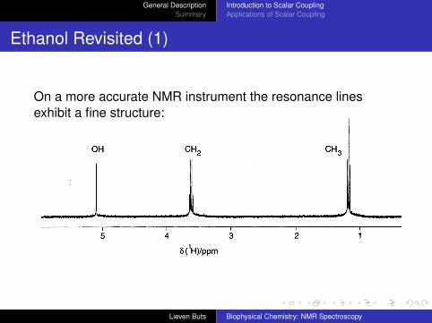
Ethanol Revisited (1)

On a more accurate NMR instrument the resonance linesexhibit a fine structure:


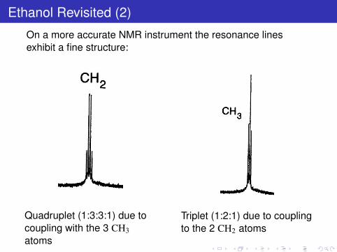
Ethanol Revisited (2)

On a more accurate NMR instrument the resonance linesexhibit a fine structure:

Quadruplet (1:3:3:1) due tocoupling with the 3 CH3atoms

Triplet (1:2:1) due to couplingto the 2 CH2 atoms



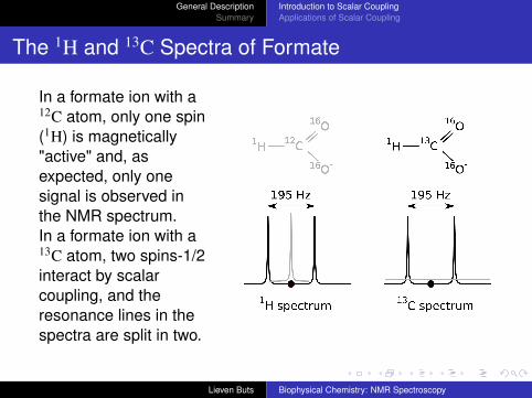
The 1H and 13C Spectra of Formate

In a formate ion with a12C atom, only one spin(1H) is magnetically"active" and, asexpected, only onesignal is observed inthe NMR spectrum.In a formate ion with a13C atom, two spins-1/2interact by scalarcoupling, and theresonance lines in thespectra are split in two.




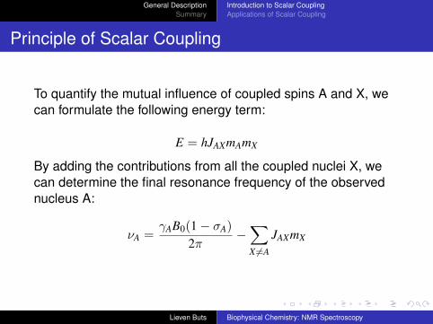
Principle of Scalar Coupling

To quantify the mutual influence of coupled spins A and X, wecan formulate the following energy term:

E = hJAXmAmX

By adding the contributions from all the coupled nuclei X, wecan determine the final resonance frequency of the observednucleus A:

νA =γAB0(1− σA)

2π−

∑X 6=A

JAXmX


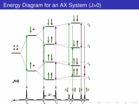
Energy Diagram for an AX System (J>0)

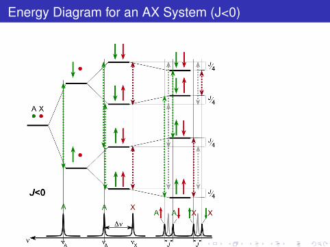
Energy Diagram for an AX System (J<0)



Mechanism of Scalar Coupling

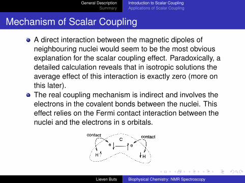
A direct interaction between the magnetic dipoles ofneighbouring nuclei would seem to be the most obviousexplanation for the scalar coupling effect. Paradoxically, adetailed calculation reveals that in isotropic solutions theaverage effect of this interaction is exactly zero (more onthis later).The real coupling mechanism is indirect and involves theelectrons in the covalent bonds between the nuclei. Thiseffect relies on the Fermi contact interaction between thenuclei and the electrons in s orbitals.




Implications of the Mechanism

The strength of the coupling effect is independent of theexternal field B0.Only covalently bound nuclei affect each other, and thestrength of the effect diminishes quickly as the number ofintervening bonds goes up.The sign of the coupling constant J is determined by thenumber of electron/electron interactions involved, whichcan be tricky to predict.




Limitations of the Basic Theory

A detailed calculation shows that the final pattern of the energylevels is determined by the difference in Larmor frequency ofthe coupled nuclei (|δν|) on the one hand, and the strength ofthe coupling (|J|) on the other hand.If |δν| >> |J|, the four energy levels remain separate, and areindeed slightly shifted as described before. Such nuclei aresaid to be weakly coupled, and the previous description worksvery well in this case.




Equivalent Nuclei (1)

When δν = 0, the αβ and βα energy levels coincide. By therules of quantum mechanics it is then possible to mix orhybridise these two levels into two new levels ( 1√

2(αβ + βα) and

1√2(αβ − βα)), which are distinct. In the weak coupling limit this

is impossible because the middle two energy levels are still toofar apart for hybridisation. The effect of the mixing is that thereare two permitted transitions at the central frequency, and twoforbidden transitions, one on either side of the center line.


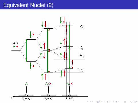
Equivalent Nuclei (2)



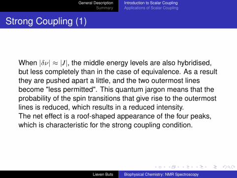
Strong Coupling (1)

When |δν| ≈ |J|, the middle energy levels are also hybridised,but less completely than in the case of equivalence. As a resultthey are pushed apart a little, and the two outermost linesbecome "less permitted". This quantum jargon means that theprobability of the spin transitions that give rise to the outermostlines is reduced, which results in a reduced intensity.The net effect is a roof-shaped appearance of the four peaks,which is characteristic for the strong coupling condition.


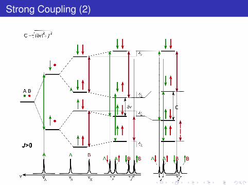
Strong Coupling (2)

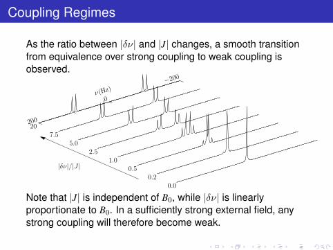
Coupling Regimes

As the ratio between |δν| and |J| changes, a smooth transitionfrom equivalence over strong coupling to weak coupling isobserved.

−200

0

200

ν(Hz)

0.00.2

0.51.0

2.55.0

7.520

|δν|/|J |

Note that |J| is independent of B0, while |δν| is linearlyproportionate to B0. In a sufficiently strong external field, anystrong coupling will therefore become weak.



Outline


2 Summary




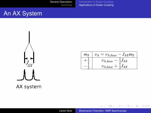
An AX System

mX νA = νA,base − JAXmX

+ 12 νA,base − 1

2 JAX

− 12 νA,base + 1

2 JAX




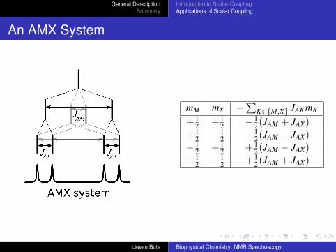
An AMX System

mM mX −∑K∈{M,X} JAKmK

+12 +1

2 −12(JAM + JAX)

+12 −1

2 −12(JAM − JAX)

−12 +1

2 +12(JAM − JAX)

−12 −1

2 +12(JAM + JAX)




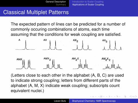
Classical Multiplet Patterns

The expected pattern of lines can be predicted for a number ofcommonly occuring combinations of atoms, each timeassuming that the conditions for weak coupling are satisfied.

(Letters close to each other in the alphabet (A, B, C) are usedto indicate strong coupling; letters from different parts of thealphabet (A, M, X) indicate weak coupling; subscripts countequivalent nuclei.)


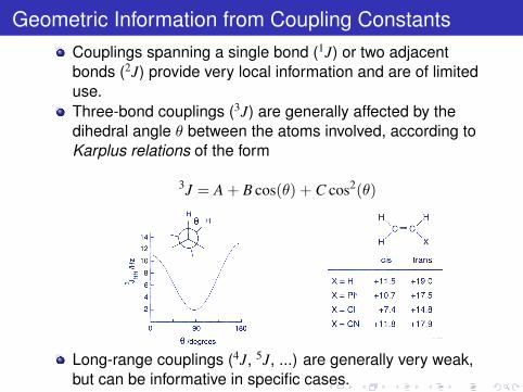
Geometric Information from Coupling ConstantsCouplings spanning a single bond (1J) or two adjacentbonds (2J) provide very local information and are of limiteduse.Three-bond couplings (3J) are generally affected by thedihedral angle θ between the atoms involved, according toKarplus relations of the form

3J = A + B cos(θ) + C cos2(θ)

Long-range couplings (4J, 5J, ...) are generally very weak,but can be informative in specific cases.



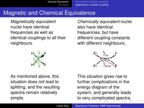
Magnetic and Chemical EquivalenceMagnetically equivalentnuclei have identicalfrequencies as well asidentical couplings to all theirneighbours.

As mentioned above, thissituation does not lead tosplitting, and the resultingspectra remain relativelysimple.

Chemically equivalent nucleialso have identicalfrequencies, but havedifferent coupling constantswith different neighbours.

This situation gives rise tofurther complications in theenergy diagram of thesystem, and generally leadsto very complicated spectra.



Summary (1)

The effect of neighbouring magnetic nuclei is describedusing the scalar coupling concept.Quantum theory describes how the energy levels of thesystem are modified by the interaction between the nuclei,changing the appearance of the spectrum.The crucial parameters are the difference in resonancefrequency between the coupled nuclei (δν, which isproportional to B0) and the strength of the scalar coupling(J, which is independent of B0).



Summary (2)

For magnetically equivalent nuclei (with δν = 0 and allother coupling constants identical) there is no net splittingof the resonance lines.For chemically equivalent nuclei (with δν = 0 but distinctcouplings with other neighbours) and for strongly couplednuclei (δν ≈ J) the resonance lines are split, reshaped andshifted. The detailed interpretation of these cases ischallenging.



Summary (3)

For weakly coupled nuclei (|δν| >> |J|) the resonance linesare split in a fairly predictable way, which can be easilyexplained in terms of the energy diagram of the spinsystem.In practical use, scalar couplings provide information aboutthe covalent structure of molecules and about specificaspects of molecular geometry.


Biophysical Chemistry: NMR Spectroscopymore.vub.ac.be/LievenButs/slides/NMR_en_3.pdfGeneral...

Documents

Transcript of Biophysical Chemistry: NMR Spectroscopymore.vub.ac.be/LievenButs/slides/NMR_en_3.pdfGeneral...