Single Versus Multi Species Indicators in Environmental Modelling: A Review

1Subana Shanmuganathan, 2Philip Sallis and 3John Buckeridge

1 & 2 Software Engineering Research Laboratory, 3 Earth and Oceanic Sciences Centre Auckland University of Technology, New Zealand. www.aut.ac.nz

(Email: subana.shanmuganathan@aut.ac.nz) Abstract The use of biological responses in environmental modelling, also referred to as biomonitoring, mainly involves indicator species or communities those accumulate pollutants in their tissues from the surrounding environment, thus reflect the environmental conditions. Despite the progress made through research activities in detecting biological changes in these organisms at various levels i.e. macromolecular, cellular within individual organisms and in communities, constraints with conventional data analysis methods in exactly assessing an environmental pollution and its real cause led ecologists to experiment with emerging technologies. The recent use of artificial neural networks (ANNs), especially self-organising map (SOM) and evolving SOM techniques to analyse multi dimensional data sets provide a means to analyse community dynamics and is elaborated upon with a case study from northern New Zealand. Introduction In this paper, we initially look into the use of single species indicators (i.e. mussels, barnacles, etc) against the multiple species or communities based indicators (i.e. intertidal, subtidal communities) in environmental modelling. Such indicator organisms enable ecologists to analyse the environment based on the levels of pollutants accumulated in these indicator organisms from the surrounding environment, (especially aquatic systems), thus reflect the environmental conditions. Hence, the use of environmental effects of ecosystems on individual organisms, either species or communities based, also referred to as biomonitoring is considered to be capable of providing information on the levels and ecological effects of the pollutants on the system being analysed. Over the years, research activities on environmental modelling based on biomonitoring techniques saw remarkable progress in detecting biological changes at various levels i.e. macromolecular, cellular, in organs within individual organisms, populations and biogeocenosis1. However, ecologists still find it difficult to exactly assess an environmental pollution and its real cause (whether human induced or due to natural or global changes) for the observed biological changes using conventional data analysis methods i.e. standard statistical data analysis methods such as analysis of variance (ANOVA), Before-After-Control-Impact (BASI) design, etc Time and again, the use of single indicator species as an indicator of a whole ecosystem has come under heavy criticisms. On the other hand communities based biomonitoring methods are found to be extremely difficult in terms of analysing the collected data using existing statistical methods. The multidimensional data collected through multi species biomonitoring techniques produce matrices of numerical values that are generally difficult to establish the exact cause of the observed biological changes. This led ecological analysts to explore latest information and data processing methodologies. Approaches based on various artificial neural network (ANN) paradigms, especially Konohen’s self-organising map (SOM) networks and their success in analysing multi dimensional data sets are elaborated upon. Finally, the use of SOMs and evolving SOMs in analysing subtidal community dynamics from northern coastal areas of Auckland in New Zealand is discussed.

“a combination on a specific area of the Earth’s surface of atmosphere, mineral strata, soil, vegetation, animal and microbial life, water - possessing its own specific type of interactions of these components and interchange of their matter and energy among themselves and other natural phenomena…” (Mackey, B. 2003).

Indicator species and communities The use of biological responses in environmental modelling is not a new phenomenon. It actually dates back to the early days of human civilisation. The latest techniques, based on the use of environmental effects of ecosystem on individual organisms, species and communities provide information on the magnitude and ecological effects of the pollutants on the system. This is despite the expensive processes involved in the initial development of such indicator systems. Basically there are two types of biomonitoring:

(i) to observe the biological system changes before and after a project is completed or before and after a toxic substance enters the water.

(ii) to ensure compliance with regulations or guidelines or to ensure water quality is maintained. (Biological Monitoring 2000). Unlike the physical and chemical indicators, biological indicators are less specific as they respond to a whole range of stressors and do not necessarily indicate the precise stressor to which they have responded. Physical and chemical indicators are highly specific and can be used for predictable stressors but may fail with unpredictable stressors (Australian and New Zealand Environment and Conservation Council November 1992). However, in light of recent advanced methods, in some cases it is even possible to detect a biological response at levels below those detectable by chemical analyses (Dixon and Pascoe, 1994 cited in (Norris 1999). Increasingly, biomonitoring is considered as a far better means in ecological studies as it allows a direct primary assessment of ecosystem conditions, something that cannot be done with dispersion models2 and instruments used in physical/chemical measurements of air quality. Overall, biomonitoring provides a first level assessment of environment health (What's Biomonitoring? 2002). Single species versus multispecies indicator concept Of all the controversies surrounding the concepts, the use of single verses multiple indicator species has been a major issue. (Soule 1988) argued that the practices based on single species concept could not be considered as a substitute for a broad-spectrum research or monitoring programs and condemned the single species concept with many examples. The requirement enforced by the US Environmental Protection Agency (EPA) and the US Army Corps of Engineers (COE) (1977) that led to the use of some species of mysid shrimp to achieve comparability for all dredge material disposal evaluations was described as a major breakthrough for the development of multispecies indicator concepts. Nonetheless, it became impractical to find species occurring both in Atlantic and Pacific coasts, as no single species occurs in all habitats. The consideration of closely related species was not possible either, because such species occupy different habitats. Thus the use of laboratory-reared species such as Mysidopsis bahia gave an alternative approach. The EPA/COE also included the use of wild or cultured crustaceans, molluscs and polychaete worm species in their requirements. This was described as a significant departure from the earlier regulations, which relied entirely on the levels of chemical pollutants in sediments without any regard to their effects on indigenous faunas. It laid the necessary foundation for the use of multiple species as representatives of different trophic levels3 or feeding guilds being gradually accepted as a necessary measure for more accurate evaluation of an environmental impact. Debate on single versus multispecies indicator concepts can be seen in many other studies as well. (Sastry and Miller 1980) who recognised the successful use of biochemical and physiological processes of aquatic organisms, based on single species concept, eventually argued that these indices might not exactly indicate whether an altered response was pollutant induced or caused by a natural environmental change. Later, even in the late 1980s a similar view was expressed by (Soule 1988) and will be further discussed in the next section (Issues with biomonitoring in environmental modelling). As the multi species concept considers only the response of a whole community (the whole assemblage of species in an area), it provides a more realistic approach and thus preferred over to the concepts on studying the fate of a selected species (Clark et al. 1997). Regardless of the claims that pointed out the pitfalls of single species indicators, plenty of applications based on single species concept were later developed and successfully used as biomonitoring devices (i.e. accumulation of certain metals in mussels, barnacles and in a few more species). The EPA’s Mussel Watch Program operated

2 “Dispersion models provides (sic) predictions as to where the pollutants will probably go most of the time and where potentially harmful depositions would most likely to occur under certain conditions. The dispersion models cannot predict where the pollutants will have an effect because they utilize no biological information that can be interpreted as susceptibility (What's Biomonitoring? 2002). 3 Trophic levels are the various levels used to define the different organisms of an ecosystem based on their positions in food chains, by which nutrients and energy move round the ecosystem in loops and cycles.

from 1976 to 1978 (Goldberg et al. 1978) with an ubiquitous bay mussel called, Mytilus edulis, found in Atlantic, Pacific and European coasts was expressed to have come close to fulfilling the single indicator organism concept. Recent single indicator species applications Single indicator species applications continued to be very much in use. In particular, the mussel watch programs became very popular as they were seen to be cost effective despite all the drawbacks reviewed, in the previous section. Even (Soule 1988), who criticised the single indicator species concept, later admitted that the mussel watch program as having satisfied the application of this concept to a greater extent. The following are a few, successful contemporary applications of mussels, as a single indicator species:

(i) The European Environment Agency used blue mussels to analyse the concentrations of lindane, zinc and cadmium in aquatic systems from 1990 to 1996 (European Environment Agency Environmental themes 2002).

(ii) The National Oceanic and Atmospheric Administration (NOAA) uses mussels and oysters to study the concentration of man made chemicals in the coastal sites of the whole nation on an annual basis. The concentrations of cadmium and other trace metals, entering the coastal waters from these chemicals i.e. DDT, PCBs, are studied through this project (O'Connor 2002).

(iii) The Vermont Department of Environmental Conservation (VTDEC), in co-operation with the Lake Champlain Basin Program members studied the zebra mussel distribution through the lake since 1994. Also produced annual reports from 1994 to 1999 period. (Lake Champlain Basin Program 2002).

(iv) The National Institute of Water and Atmosphere (NIWA), in New Zealand developed techniques for environmental monitoring studies using freshwater mussels for lake and river habitats. The techniques were found to be useful in assessing the pollution impact for the environmental impact assessment information required under the Resource Management Act. With the use of both measurements, the chemical contaminants together with biological responses in mussels, NIWA was able to assess the effects of pollutants on mussel health. Consequently, they developed an on-line electronic system capable of continuously measuring the valve movement response; a real-time biomonitoring device for use in environments, receiving highly time varying pollutants i.e. storm water discharges (Hickey 2000).

With that brief history on the controversies surrounding the single versus multispecies indicators in environmental modelling, in the next section the latest biomonitoring methods and related issues are discussed. Developments in Biomonitoring Over the years, research activities in environmental modelling based on biomonitoring techniques saw considerable progress in detecting biological changes at various levels. Despite this success, ecologists often find it difficult to exactly assess an environmental pollution and its real cause. A hypothetical model (figure1) based upon (Sastry and Miller 1980), illustrates the time related sequence of possible effects of reduced water quality either pollutant induced or due to natural causes, at various levels of biological organisation. The major identified problem in pollution monitoring of the 1980s, was the inability to distinguish a response, whether arising from environmental or natural causes. More than two decades on, the situation remains the same and is elaborated upon hereon. Issues with biomonitoring in environmental modelling In spite of the development and broad use of biomonitoring practices to study the environmental conditions, a symposium held in the late 1980s on this subject by the Southern California Academy of Sciences had a number of issues to deal with. Many questions were raised on the concept and the ‘rules’ administered for appropriate use of these organisms to particular problems:

(i) How would the true indicators be distinguished from biological anomalies? (ii) How would one select the kinds of organisms that would be appropriately associated with

conditions and events at various scales in time and space? (iii) To what extent would any one particular species represent other species in the same environmental

setting? (iv) Could the indicator concept be applied to modern sampling and analytical technology? (v) How would the anthropogenic disturbances be distinguished from those of natural phenomena? (vi) How would the differing databases be best matched with deferring scales?

(Soule and Kleppel 1988). A recent website of (National Center for Environmental Research (NCER) Office of Research and Development attached to United States EPA 2001) consists of a list of science questions and issues, addressed by this body on the impact of ecological assessment and indicators: “…How Can We Identify and Develop Molecular and Cellular Indicators for Monitoring and Assessing Changes in Genetic Diversity in Response to Environmental Stress? How Can We Relate Indicators of Population and Community Structure and Function to Exposure to Chemical, Physical and Biological Stressors? How Can We Assess Ecological Condition Through Chemical Indicators? How Can We Use Remote Sensing Techniques to Develop Landscape Indicators that Quantify and Characterize the Geographic Extent of Key Attributes as They Relate to a Range of Environmental Values? How Can We Assess Ecological Condition Using Indicators that Incorporate Multiple Resources and Spatial Scales? …” (National Center for Environmental Research (NCER) Office of Research and Development (ORD) - US Environmental Protection Agency (EPA) 2000:1)

Figure 1: A hypothetical time related sequence of possible biological effects of reduced water quality. Source: (Sastry and Miller 1980:267)

As explained in the initial part of this section, the symposium held in the mid 1980s on biomonitoring practices to study ecosystem conditions by the Southern California Academy of Sciences expressed concerns over the use of biological indicators to analyse the environmental conditions (Soule and Kleppel 1988). Two decades on, the concerns and issues remain the same, as seen in (National Center for Environmental Research (NCER) Office of Research and Development attached to United States EPA 2001) as well as in (Graedel et al. 2001). It appears then, even today as far as ecosystems issues are concerned, the uncertainties remain the same; except for some changes in the terminology despite the advances of science and technology. In fact, the more we learn about ecosystems the greater the complexity revealed. This is surprising in considering the amount investment made by industry, government and academic research in reviewing, debating and complying with countless number of environmental regulations world wide, and still faced with considerable uncertainty on the consequences of human induced impact, particularly in marine habitats as argued in (Osenberg and Schmitt 1996). The major issues for this could be

(i) (ii)

the inherent complexities of ecosystem structure and functioning, and the twentieth century approaches, based on gaining in-depth knowledge that led to decision making and actions with a fragmented image of nature (Bowler 1992).

For the purpose of improving our understanding on ecosystems, to use them while preserving their natural characteristics and biodiversity from human influenced impact, (Graedel et al. 2001) selected several areas as imperative for future research. The following were among the topics, mainly focused on biodiversity (i.e. community structure and its dynamics) to gain knowledge on ecosystem functioning:

(i) Development of improved tools for rapid assessment of diversity at all scales. (ii) Work on producing a quantitative, process-based theory of biological diversity at the largest

possible variety of spatial and temporal scales. (iii) Work on elucidating the relationship between diversity and ecosystem functioning. Produce

developing and testing techniques for modifying, creating and managing habitats that can sustain biological diversity as well as people and their activities.

Of the above four selected areas for immediate research investments, the following was the recommendation made for biological diversity and ecosystems functioning: “Recommendation: Develop a comprehensive understanding of the relationship between ecosystem structure and functioning and biological diversity. This initiative would include experiments, observations and theory and should have two interrelated foci: (a) developing the scientific knowledge needed to enable the design and management of habitats that can support both human uses and native biota; and (b) developing a detailed understanding of the effects of habitat alteration and loss on biological diversity, especially those species and ecosystem whose disappearance would likely do disproportionate harm to the ability of ecosystem to meet human needs or set in motion the extinction of many other species.” (Graedel et al. 2001:5). Latest developments in biomonitoring The currently adopted, popular biomonitoring methods, involving the use of biological responses are still either based on the use of indicator species or indicator communities; both at different levels and scales i.e. macromolecular, cellular, using organs, organisms, population and biogeocenosis. The recent indicator species level methods (based on single indicator species applications) are seen to be more advanced with abilities to analyse biochemical, histological, morphological and physiological changes in individual organisms; but only in certain specific organisms i.e. filter feeders such as clams and mussels. These changes are then related to the identified environmental stressors, as explained in Sastry’s (1980) model; thus using these organisms as true indicators or biomonitoring devices of environmental changes. Such organisms are sometimes referred to as sentinel organisms in recent studies. The use of modern techniques in cell biology led to further improvements in the analysis of environmental pollution with indicator organisms. With the new methods, analysts are able to find the amount of certain contaminants, in cells of different ages within the same tissue of an individual organism. The concentrations of a specific contaminant in such different aged tissues/cells are used to determine the history of the contaminant in a particular environment. The accumulation of specific contaminants in certain specific organisms, especially in filter feeders and bivalves (i.e. clams and barnacles), in their gills has been well analysed and documented (Phillips and Rainbow, 1993 Biological Monitoring, 2000). Even certain algal species as well are used in this type of biomonitoring measures. The following are some sentinel organisms listed along with their respective contaminants, established through research:

Extreme Uptake Barnacles Zinc (Zn) Bivalve molluscs Copper (Cu), iron (Fe), manganese (Mn), lead (Pb), Zn Gastropod molluscs Cu, Zn Isopods, amphipods Cu, Fe, Pb, Zn Polychaetes Cu

Moderate Uptake Macroalgae (seaweeds) Most metals Mussels/other bivalves Metals, metallothioneins Polychaetes Cadmium (Cd), Pb Decapods (crayfish) Cd, Pb Finfish Cd, Pb (Biological Monitoring 2000) (Adapted from Phillips and Rainbow, 1993) The following is a model that provides an overview on the levels of organisation and their associated biomonitoring measures of recent times:

(i) Individual - Organism - genetic mutations - reproductive success - physiology - metabolism - oxygen consumption, photosynthesis rate - enzyme/protein activation/inhibition - hormones - growth and development - disease resistance - tissue/organ damage - bioaccumulation

(ii) Population - survival/mortality - sex ratio - abundance/biomass - behaviour (migration) - predation rates - population decline/increase

(iii) Community - Abundance ("evenness") of an organism or organisms - Biomass - Density of an organism or organisms - Richness (variety) - number of species, size classes, or other functional groups, per unit area or volume, or per number of individuals. - Diversity - the richness given the relative abundance of each species or group.

(iv) Ecosystem - Mass balance of nutrients. (Adams and Brandt, 1990) cited in (Biological Monitoring 2000). Recent efforts in integrated analysis In recent years, especially since the last decade on, the development of integrated data analysis methods for ecosystem system modelling in order to inform sustainable environmental management has regained momentum. Many academic and research institutions have initiated research in a wide range of disciplines to develop integrated approaches for ecosystem modelling with funding from (National Center for Environmental Research (NCER) Office of Research and Development (ORD) - US Environmental Protection Agency (EPA) 2000). The research carried out during the last two years, aimed at developing a new suite of environmental integrative indicators for use in estuarine and other long-term environmental monitoring programs could be seen under various topics at http://es.epa.gov/ncer/starreport.html. The details in the websites illustrate the scope of the research carried out, extending from DNA analysis to integrated ecosystem modelling techniques with interfaces to geographical information systems (GISs). The need for integrated data analysis methods have been stressed in many recent articles as well (Mann 1982; Harris 2002; Parker et al. March 2001); it appears that the problems in introducing integrated research approaches for ecosystem analysis also have remained the same since the early 1980s until recent times. The following is an outline on the attempts made by ecologists and academic researchers in developing effective and efficient environmental indicators for sustainable ecosystem management in New Zealand’s perspective. The new criteria show a shift in which more emphasis is made towards the protection of ecosystems (Norris 1999). The following are the guidelines (i.e. three key elements) set out for developing useful indicators to assess the environmental conditions in New Zealand and Australia; an indicator should,

(i) be more ecosystem specific, rather than focusing on human health as in the past, (ii) be more focused on the actual issues or problems caused by physical, chemical and biological

stressors rather than on individual indicators and (iii) be risk based. The new approach aims to develop guideline ‘packages’ with key performance

indicators and trigger levels in these indicators, for each issue and wherever possible for each ecosystem type.

The following are the requirements suggested for an effective environmental indicator based upon (Norris 1999); it should,

(i) be able to quantify and simplify the complex phenomena

(ii) have scientific validity, operational at appropriate geographic scales (iii) be able to respond predictably to environmental changes (iv) be easy to understand (v) be forward looking or predictive.

The perceived inadequacies with conventional methods in identifying a useful environmental indicator to predict ecosystem dynamics have been revealed in many studies. All of the past and present methods fall short in accurately defining the ecosystem response to human activities in a simple, easily understandable format and (Norris 1999) blamed method design for this, citing many earlier studies (Eberhardt 1963, 1976; Green 1979; Waters and Resh 1979; Ellis and Lacy 1980; Carins and Pratt 1986;Norris and George 1986; Cooper and Barmuta 1991). All of them had repeatedly stressed the need for good study design with clearly set objectives. (Mann 1982) was correct; the models of the 1980s were good at providing some means for gaining insight into ecosystem complexities, but not for the prediction of ecosystem behaviour as needed for resource management purposes. Even after two decades, the issues still remain the same. In a nutshell, ideal environmental indicators should be able to point out a more complex situation as seen in other fields i.e. GDP, stock market indices, etc of the financial sector; instead of scientists making measures with sophisticated equipment and writing highly technical reports with complex formulae and solutions that are generally incomprehensible by other professionals. Multispecies or community based indicators Multispecies or community based indicator studies consist of complex multivariate analytical techniques to analyse the relationships between environmental parameters and the biological data. The use of benthic organisms of marine habitats to analyse the environment using this concept is explained herein based upon (Smith et al. 1988) . The multivariate analytical techniques simultaneously consider more than one single dependent variable in the analysis, whereas univariate methods consider only a single variable at a time. All methods discussed here are based on an approach (figure 2) that consists of three main steps:

(i) In the first step the biological data is analysed separately to determine the community patterns. (ii) In the second step the environmental data is prepared in a format suitable for use in the next step. (iii) In the third and final step the community patterns determined in the first step are related to the

environmental factors.

Step 1: Community patterns in the hypothetical biological data representing benthic grab samples taken at several points i.e. along a chosen offshore transect at different depths, increased by 10 metres, are determined in this step with the use of dissimilarity index. The indices such as similarity and dissimilarity are used to quantify the community relationships between pairs of samples. A pair of samples that consists of similar species composition and abundance will be assigned a relatively low dissimilarity value and conversely assigned a relatively high similarity value. Hence, similarity and dissimilarity indices actually describe the same fact, except for the direction of measure, which is opposite. There are some shortcomings in this method; the most important issue is that after a point the dissimilarity values approach an asymptote as the samples being compared show greater amounts of biological change (Beals, 1973 cited in Smith, 1988). At a point where there are no species in common in the two samples being compared, the dissimilarity index value reaches the maximum and the biological changes beyond this point could not be measured by any further increase in dissimilarity. To overcome the asymptote problem Williamson (1978) and Smith (1984) cited in (Smith 1988) suggested the step-across procedure, where the longer dissimilarity values are re-estimated from the shorter dissimilarity values. The ZAD dissimilarity index (Mahon et al, 1984; Stull et al, 1986 cited in Smith, 1988) is one among the few other methods, recommended to overcome this problem. The use of dissimilarity matrix to determine the community patterns has limited interpretation values. Thus cluster analyses and ordination techniques that utilise dissimilarity matrix as their starting point, are suggested to better delineate the community patterns in the data. Ordination analysis: Ordination analyses are generally used to display the biological patterns in a multidimensional space using the calculated dissimilarity indices. The distance between any two data points would be proportionate to their dissimilarity factor and the axes represent the dimensions of the space. The

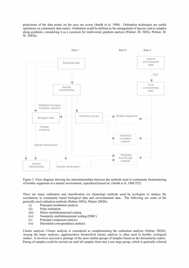
projections of the data points on the axes are scores (Smith et al. 1988). Ordination techniques are useful operations on community data matrix. Ordination could be defined as the arrangement of species and/or samples along gradients, considering it as a synonym for multivariate gradient analysis (Palmer, M. 2002a :Palmer, M. W. 2002b).

Step 1 Step 3 Step 2

Weighted discriminate

analysis

Canonical correlation analysis

Multiple regression

Sample dendrogram

Species dendrogram

Flexible clustering

Weighted averages, Euclidean distance

Final environmental

data

Original environmental

data

Sample dissimilarities

Biological data Ordination scores

Sample dissimilarities

Biological data

PCA

Figure 2: Flow diagram showing the interrelationships between the methods used in community biomonitoring of benthic organisms in a marine environment, reproduced based on: (Smith et al. 1988:252)

There are many ordination and classification (or clustering) methods used by ecologists to analyse the correlations in community based biological data and environmental data. The following are some of the generally used ordination methods (Palmer 2002a; Palmer 2002b):

(i) Principal coordinates analysis (ii) Polar ordination (iii) Metric multidimensional scaling (iv) Nonmetric multidimensional scaling (NMC) (v) Principal component analysis (vi) Detrended correspondence analysis

Cluster analysis: Cluster analysis is considered as complementing the ordination analysis (Palmer 2002b). Among the many analyses, agglomerative hierarchical cluster analysis is often used in benthic ecological studies. It involves successive pairings of the most similar groups of samples based on the dissimilarity matrix. Paring of samples could be carried out until all samples form into a one large group, which is generally referred

to as a ‘dendrogram’. A two-way coincidence table facilitates the task of choosing the groups from a dendrogram. Step 2: In the next step the environmental data is converted into formats to depict correlating patterns within that of the biological data. The multivariate analytical methods used to correlate the environmental and community patterns are data dependent and may produce misleading, confusing, unstable or incomputable results. The main problems that may arise from environmental variables are as follows:

(i) The presence of very high interrelations (multi co-linearity) between any two environmental variables. When the correlation between any two variables equals to one, it becomes impossible to compute the results. As the number of such variables increases, the incidence of such problems also increases.

(ii) Predictability of a variable from a linear function of any one of the other variables makes the results incomputable. If and when the relationships between the variables become completely predictable, the results become ill determined.

(iii) The use of excessive number of variables in the analysis increases the chances of increased combination of ecologically meaningless variables and their emphasis in the results.

(iv) The use of inadequate sample size; when the number of environmental variables approaches the number of samples, the results become incomputable.

(v) Measurement error in the environmental data can be magnified by any of the above-mentioned problems.

(Smith et al. 1988). Principal component analysis: Principal component analysis (PCA) is an ordination technique, in which a new composite environmental variable is created from the original set of environmental variables. This process is expressed to be useful in eliminating the above-mentioned problems. The scores on each PCA axis are new environmental variables. Thus the meaning of these new scores could be studied from the correlations between the original environmental variables and the scores for the axis, and it is important that the new environmental variables from the PCA are interpretable. In addition, the following measures are advised to avoid some of the above-mentioned problems (numbered (i)-(v)) that arise from two or more environmental variables being used to measure the same factor;

(i) to remove all variables that are used to measure the same environmental factor leaving just one (ii) even if such variables do not show a high correlation, a variable that represents the factor better be

retained in favour of the others. This helps in reducing the number of variables. Step 3: In this step, as environmental gradients are considered to cause changes in the community, the community patterns expressed by the scores on the ordination axes will be correlated with the environmental gradients. Need of innovations The multispecies or community biomonitoring methods that belong to a hypothesis testing class of analysis are very much included in BASI designs. ANOVA is also a multivariate analysis method used in community biomonitoring studies. Both, commonly used in academic and highly technical studies, are considered to be rigorous data analysis methods. However, in recent years the soundness of these methods has been questioned and challenged by land developers; their inability to produce conclusive results has earned the ignorance of stakeholders and the general public on scientific findings and predictions. In concurrent, our lack of knowledge on ecosystem structure and functioning is seen as the main reason for the flaws in assessing current environmental problems and their exact cause. Furthermore, scientists’ approaches of the late twentieth’ century, based on hypothesis postulation and testing to gain in-depth knowledge, leading to subdivisions of the earth’s image, are increasingly being criticised. Many studies, reviewed so far in this paper revealed these issues. Conversely, data mining techniques that belong to an exploratory data analysis class i.e., the exploration of novel patterns and relationships within the input vectors even with no prior knowledge, are seen to be more suited for analysis of monitoring data. The findings of exploratory analyses may be then used for hypothesis postulation and testing. Hence, exploratory data analyses (quantitative analyses) could serve better to analyse the current issues, as they provide a means to investigate for new trends in the multidimensional monitoring data sets even with our limited knowledge on ecosystems. Artificial neural networks and applications to real world problems

Even though artificial neural networks (ANNs) have been around since the invention of early computers, their applications to real world problems have not been spectacular throughout. However, expectations from computers and ANNs have been steadily growing. “…In 40 years’ time people will be used to using conscious computers and you wouldn’t buy a computer unless it was conscious…” (Aleksander 2000:1). Indeed such inspirations play a significant role for the incorporation of innovations and flexibility in devising intelligent systems (ISs) for increasingly complex information processing. The late 1970s’ biologically inspired ANN models, also referred to as connectionist paradigms provided a means to introduce heuristics to conventional computing methodologies and paved the way for innovative applications across a wide spectrum of disciplines. The late 1990s’ approaches of intelligent information processing methodologies, of course provide ways and means for solving more modern day complex problems such as speech recognition, image processing, modelling of complex industrial processes and information processing systems (i.e.. intelligent agents, etc.,). An artificial neural network (ANN) consists of basic elements called neurons that are loosely based on biological nerve and the brain cells. The neurons of a network are connected to each other with weights defined to them. Depending on the architecture of a network, summation function, and learning and recall algorithms used, an ANN could be trained to solve problems that cannot be solved by conventional computing techniques, which need step-by-step instructions to solve a problem. During the training process problems and their solutions are stored in the network based on the training algorithm being used. When similar problems are presented to the trained network it is able to produce the solutions based on the recall algorithm being implemented i.e. once a network is trained to learn the relationships between the input and the output it is able to produce the output for similar input values because of its generalisation abilities. In the last decade, algorithms also have been developed to extract knowledge from a trained network in the form of rules. In mathematical terms ANN applications could be described as fitting a line or curve through a set of data points. ANN applications in ecological modelling The use of ANNs in environmental sciences has been remarkable since the late 1990s despite the initial scepticism caused due to lack of knowledge. During the last couple of years alone many scientific papers have been published on ANN applications in ecological modelling, as they are seen to be successful in producing prediction models to inform sustainable environmental management. Presently there are many conferences that are solely dedicated for ecological informatics i.e., (3rd conference of the International Society for Ecological Informatics - http://www.isei3.org/index.htm#top). Self-organising maps A Self-organising map (SOM) is a feed forward neural network (figure 3 c), which uses an unsupervised training algorithm to perform non-linear regression. Through a process called self-organisation the network configures the output data into a display of topological representation, where similar input data are clustered near to each other. At the end of the training SOM enables analysts to view any novel relationships, patterns or structures in the input vectors. The topology preserving mapping nature of SOM algorithm is highly useful in projecting multi dimensional data sets into low dimensional displays, generally into one- or two-dimensional planes. Thus SOMs can be used for clustering as well as visualisation of multi dimensional data sets. Traditional methods (i.e. simple statistical methods) are very useful in summarizing low-dimensional data sets (mean value, smallest, highest values, etc.,). However, they cannot be successfully used to analyse or visualise multi-dimensional (i.e. multivariate) data sets (Deboeck and Kohonen 1998) The self-organising map (SOM) algorithm, first introduced by Tuedo Kohonen (1982) was developed from the basic modelling information of the human brain’s cortical cells, as they were known from the neuro-physiological experiments of the late twentieth century. The processing of synaptic connections between the cortex cells in the human brain is based upon the nature of the sensorial stimuli. The different patterns of sensorial signals converge at different areas within the brain’s cortex cells. Thus different individual neurons or groups of neurons become sensitive to different sensorial stimuli. Neighbouring neurons also learn to respond to similar patterns of signals (figures 3 a & b) i.e. visual, auditory, somatosensory, etc. The basic SOM algorithm was developed based on this concept (Kohonen 1997).

Figure 3 a, b and c: Brain areas and somatosensory map Source: (Kohonen 1997) c: Simplified SOM diagram. The SOM methods are successfully used in exploratory data analysis/ data mining4. The following are the contributing factors of a SOM method for this:

(i) It is a numerical instead of symbolic method. (ii) It is a non-parametric method. (iii) No need for prior assumptions on the distribution of data or the analysis (iv) It is a method that can detect unexpected structures or patters by learning without supervision.

(Deboeck 1998) An algorithm of evolving self-organizing map (ESOM), where the network structure evolves in an on-line adaptive mode was introduced by (Deng and Kasabov 1999). This model consists of abilities to explore large amount of data flows, updated daily, hourly or every minute. Extracting knowledge from such large and continuously changing data sets, received in an on-line environment, could be of invaluable use for future decision-making, i.e. macroeconomic performance of individual countries or country clusters. In the next part, the use of SOM and ESOM to analyse multispecies biomonitoring data from northern New Zealand is elaborated. Auckland Regional Council (ARC) monitoring data ARC began conducting sub and intertidal biological monitoring programmes to study the effects of urbanisation on the marine habitats of the Waitemata Harbour and northeastern coasts of Auckland in New Zealand. The main aim of the programme was to analyse the population dynamics (i.e. species composition changes in the monitoring data), to study the environmental change of the coastal systems under study. Initially, the programme was limited to Long Bay only, but eventually was extended to cover areas from Campbell Bay to Waiwera (figure 4), fulfilling the BACI design method requirement; to see whether the Long Bay’s species composition changes were confined only to its coastal systems, affected by the urbanisation in near shore. Researchers of the University of Auckland (UoA) based at the Leigh Marine Laboratory have been carrying out the monitoring programmes for ARC, since 1998. For more information on data collection methods and analyses used, the original report (Walker et al. 2000) should be consulted. SOM analysis and Methodology Of the above monitoring data collected by UoA research staff, only the subtidal species composition changes (consisting of 42 species count average of the 30 sites from six beaches Campbells bay, Torbay, Long Bay, Manly, Stanmore and Waiwera of figure 4) along with sedimentation data are analysed with SOMs and ESOM in this paper. “'Data mining' or 'exploratory data analysis' generally refers to knowledge discovery, the whole process of discovery of novel patters or structures in the data. At the first international conference in Montreal in 1995, it was proposed that the term 'knowledge discovery' be employed for describing the whole process of knowledge extraction (knowledge means relationships and patters between data elements) from data and ‘data mining’ be used exclusively for the discovery stage of the process (Deboeck and Kohonen 1998b)

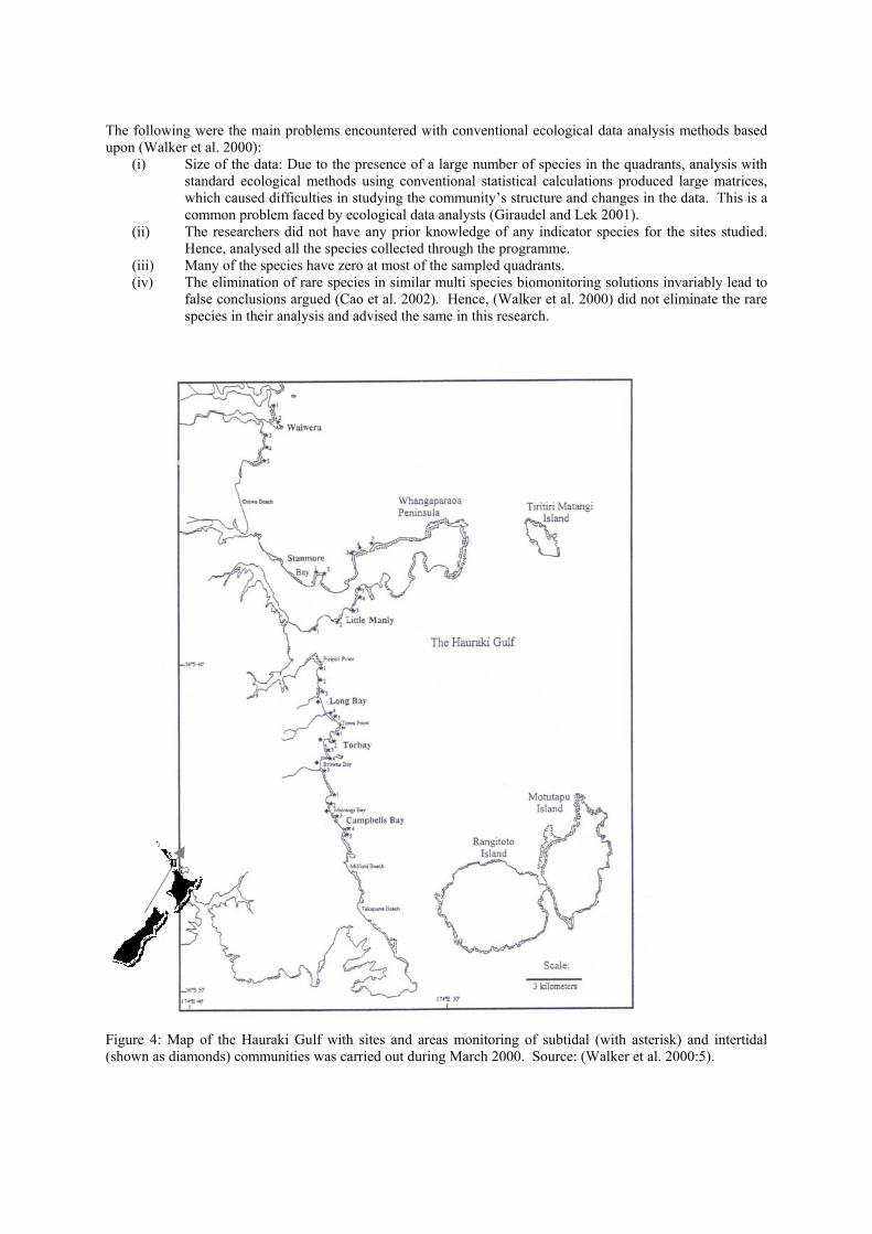
The following were the main problems encountered with conventional ecological data analysis methods based upon (Walker et al. 2000):

(i) Size of the data: Due to the presence of a large number of species in the quadrants, analysis with standard ecological methods using conventional statistical calculations produced large matrices, which caused difficulties in studying the community’s structure and changes in the data. This is a common problem faced by ecological data analysts (Giraudel and Lek 2001).

(ii) The researchers did not have any prior knowledge of any indicator species for the sites studied. Hence, analysed all the species collected through the programme.

(iii) Many of the species have zero at most of the sampled quadrants. (iv) The elimination of rare species in similar multi species biomonitoring solutions invariably lead to

false conclusions argued (Cao et al. 2002). Hence, (Walker et al. 2000) did not eliminate the rare species in their analysis and advised the same in this research.

Figure 4: Map of the Hauraki Gulf with sites and areas monitoring of subtidal (with asterisk) and intertidal (shown as diamonds) communities was carried out during March 2000. Source: (Walker et al. 2000:5).

The following are the measures taken to overcome the above-motioned problems:

(i) Visovery® SOMine lite version 4.0 by eudaptics software gmph package, commercial data depiction software, is used to create SOM maps as it has the capacity to handle up to 50 variables.

(ii) Initially the average counts of all 42 species, calculated from the collected data covering a period of three years from 1999 to 2001 are used in the SOM analysis.

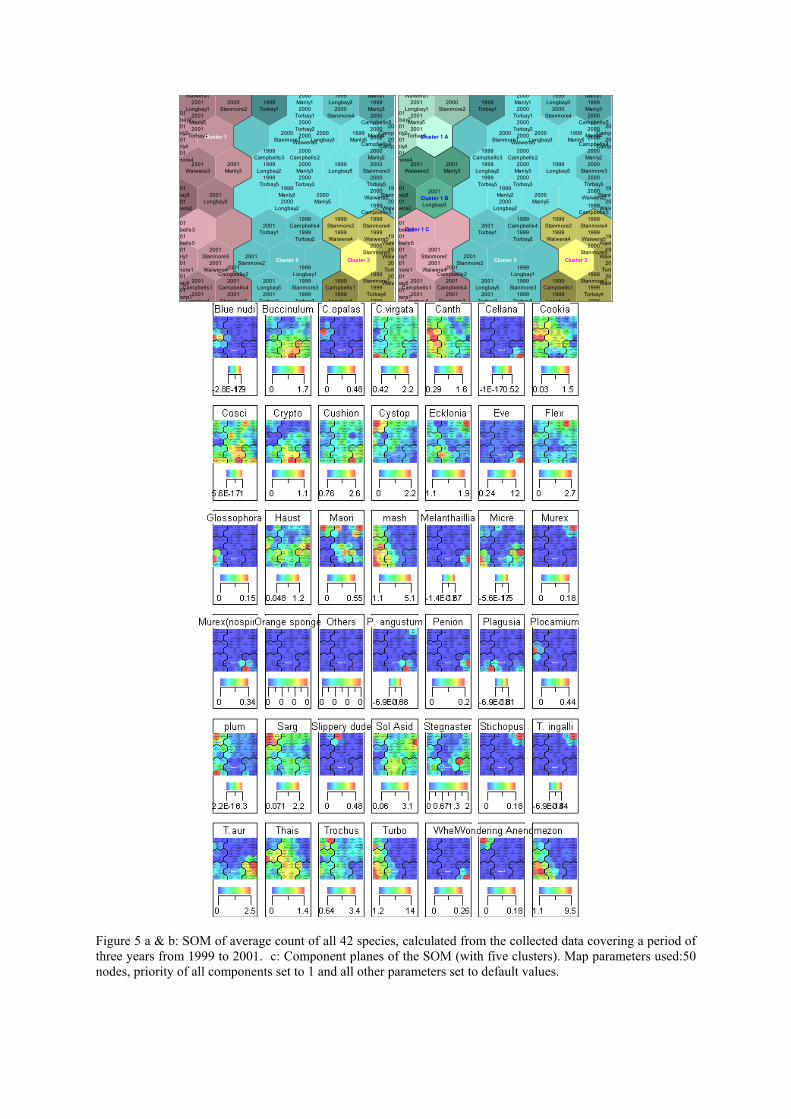
Later, count average data on 25 species, selected by (Walker et al. 2000) is analysed without and with sedimentation data from the same monitoring programme. This is done to see whether species average count data alone could be used to find the variation caused by sedimentation arising from urbanisation on North Shore. If proven this would significantly facilitate the design of biological indicators based on subtidal population dynamics to analyse the effects of urbanisation on coastal and marine life at Long Bay and the other beaches along the coast. Results and discussion Initially a SOM (figures 5 a and b) was created with the 42 subtidal species average count data, from the 30 cites (5 cites from each of the six beaches selected along the north eastern coast of Auckland), from 1999 to 2001. SOMs displayed the variables on highly visual formats through which the analysis was enhanced significantly. Viscovery’s abilities also show potential for developing prediction models on the subtidal population dynamics with simulated sedimentation data. The following is a summary of the observations made in the SOM map (figures 5 a b & c):

(i) In the SOM, the clustering has picked up the annual variations among beaches: Cluster 1 with many of the year 2000 beach sites, cluster 2 with many of the year 2001 site data and cluster 3 with many of the year 1999 data. However, the percentage of 2001 beach sites in cluster 2 is seen prominent than that of 2000 and 1999 in clusters 1 and 3 respectively. This leads to the conclusion that the deviation in year 2001 is more than that of annual. SOM cluster data superimposed on a GIS Arc View 8.2 (figure 6 d) illustrates this fact.

(ii) When divided into five clusters, cluster 2 was further subdivided into three cluster; 2A, 2B and 2C, all five sites of Campbells bay for year 2001 falling in the left bottom corner, in cluster 2C. It could be interpreted as the inter beaches variations as more than that of inter annual.

In the next stage a SOM was created with the summarised list of 25 species average count data for the six beaches covered in the monitoring programme with (figures 6 a b & c) and with sedimentation data and the interpretations arrived at are:

(i) All the beach data points were separated into 3 major clusters with the year 2001 data in the left side on both maps. Similarly, most of the year 1999 points were gathered in the centre along with the year 2000 data in the right side of the maps. Stanmore 1999 is seen alone in one cluster. This shows that the annual variations among the subtidal population dynamics along these beaches can be differentiated with SOM cluster analysis.

(ii) When divided into five clusters, year 2001 cluster got further divided into three divisions. It could be interpreted that the variations among beaches in year 2001 as higher than that of experienced in the earlier years.

(iii) Of the five beaches Campbells bay 2001 and Long bay 2001 fall into different clusters. All the other sites Manly, Torbay, Stanmore and Waiwera for 2001 fall into one cluster. In figure 6 b, all 5 sites of Champbells bay fall in 2C

(iv) Arrows in figure 6 b show the trajectory for each and every beach over the three year period monitored.

Waiwera12001

Longbay12001

Manly52001

Torbay4

2000Stanmore2

1999Torbay1

2000Manly12000

Torbay12000

Torbay22000

Waiwera5

1999Longbay3

2000Stanmore4

Manly11999

Manly32000

Campbells52000

Manly4

01bay201nly201nly401

more4

2000Stanmore1

2000Longbay3

1999Manly5

20Camp

20Camp

2001Waiwera3

2001Manly3

1999Campbells3

1999Longbay2

1999Torbay5

2000Campbells2

2000Manly32000

Torbay3

1999Longbay5

2000Campbells4

2000Manly22000

Stanmore32000

Torbay52000

Waiwera2

01bay301

wera2

2001Longbay3

1999Manly22000

Longbay2

2000Manly5

19Stanm

20Waiw

2001Torbay1

1999Campbells4

1999Torbay2

1999Stanmore2

1999Waiwera4

1999Campbells5

1999Stanmore4

1999Waiwera5

2000Stanmore5

01bells301bells501nly101

more101

bay501

wera1

2001Stanmore5

2001Waiwera4

2001Stanmore2

19Waiw

19Waiw

20Torb

20Waiw2001

Campbells12001

Longbay4

2001Campbells2

2001Campbells4

2001Stanmore3

2001Longbay5

2001Torbay2

1999Longbay1

1999Stanmore3

1999Torbay3

1999Campbells1

1999Longbay4

1999Stanmore1

1999Torbay4

1999

Cluster 1

Cluster 2 Cluster 3

Waiwera12001

Longbay12001

Manly52001

Torbay4

2000Stanmore2

1999Torbay1

2000Manly12000

Torbay12000

Torbay22000

Waiwera5

1999Longbay3

2000Stanmore4

Manly11999

Manly32000

Campbells52000

Manly4

01bay201nly201nly401

more4

2000Stanmore1

2000Longbay3

1999Manly5

20Camp

20Camp

2001Waiwera3

2001Manly3

1999Campbells3

1999Longbay2

1999Torbay5

2000Campbells2

2000Manly32000

Torbay3

1999Longbay5

2000Campbells4

2000Manly22000

Stanmore32000

Torbay52000

Waiwera2

01bay301

wera2

2001

Longbay3

1999Manly22000

Longbay2

2000Manly5

19Stanm

20Waiw

2001Torbay1

1999Campbells4

1999Torbay2

1999Stanmore2

1999Waiwera4

1999Campbells5

1999Stanmore4

1999Waiwera5

2000Stanmore5

01bells301bells501nly101

more101

bay501

wera1

2001Stanmore5

2001Waiwera4

2001Stanmore2

19Waiw

19Waiw

20Torb

20Waiw2001

Campbells12001

Longbay4

2001Campbells2

2001Campbells4

2001Stanmore3

2001Longbay5

2001Torbay2

1999Longbay1

1999Stanmore3

1999Torbay3

1999Campbells1

1999Longbay4

1999Stanmore1

1999Torbay4

1999

Cluster 1 A

Cluster 2 Cluster 3

Cluster 1 B

Cluter 1 C

Figure 5 a & b: SOM of average count of all 42 species, calculated from the collected data covering a period of three years from 1999 to 2001. c: Component planes of the SOM (with five clusters). Map parameters used:50 nodes, priority of all components set to 1 and all other parameters set to default values.

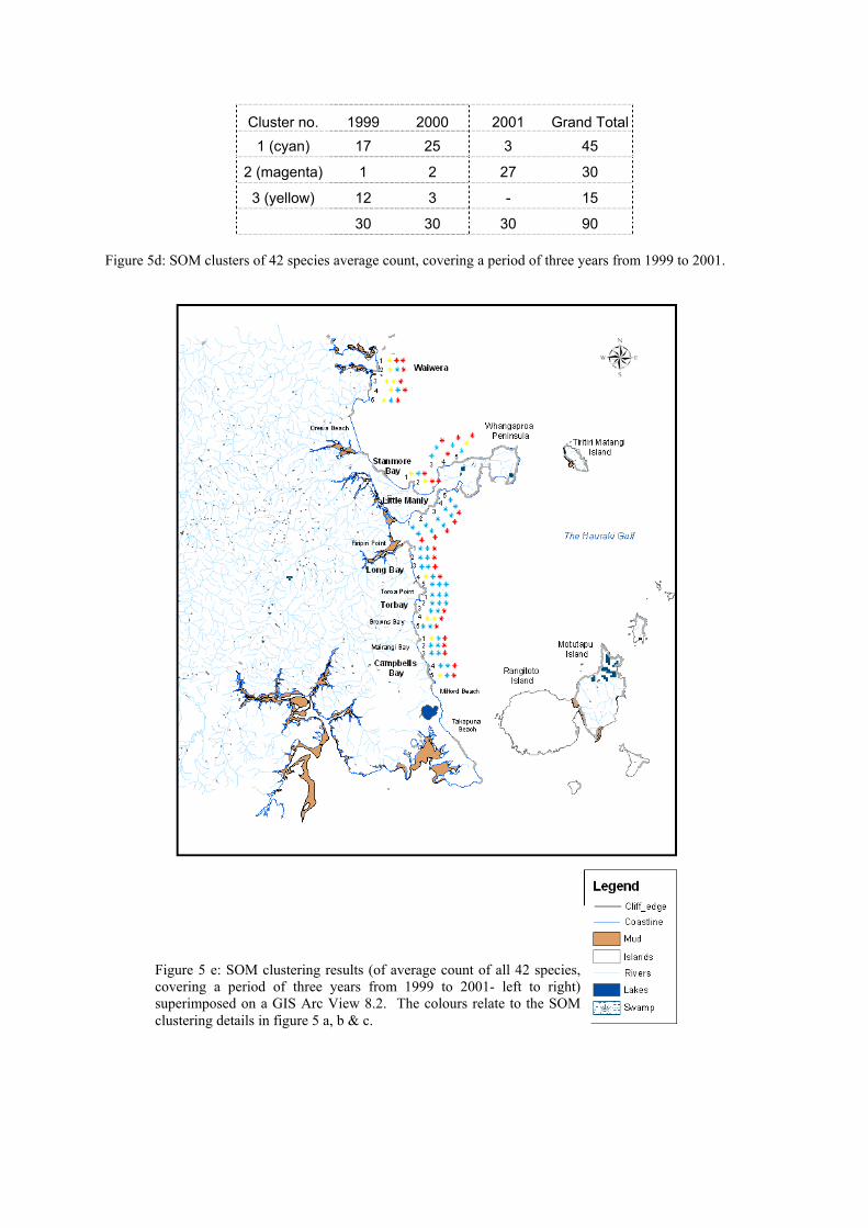
Cluster no. 1999 2000 2001 Grand Total 1 (cyan) 17 25 3 45

2 (magenta) 1 2 27 30

3 (yellow) 12 3 - 15

30 30 30 90 Figure 5d: SOM clusters of 42 species average count, covering a period of three years from 1999 to 2001.

Figure 5 e: SOM clustering results (of average count of all 42 species,covering a period of three years from 1999 to 2001- left to right)superimposed on a GIS Arc View 8.2. The colours relate to the SOMclustering details in figure 5 a, b & c.

Figures 6 a, b and c: SOM map created with the summarised list of 25 species average count data with sedimentation data. Map creation parameters: 50 nodes priority of all components set to 1 and all other map parameters set to default values. a: three cluster, b: five clusters and c: components map. In order to confirm the correlations between the observed sediment deposition rates and the subtidal species average count data from the above SOM analyses, significance tests were carried out and the following species showed significant correlation at less than 0.05p value; Flex -0.250 0.159 -0.045 -0.157 0.172 -0.114 0.026 -0.130 0.025 0.158 0.674 0.140 0.104 0.284 0.805 0.220 mash 0.535 0.120 0.208 0.057 0.039 0.149 0.322 -0.084 0.000 0.289 0.049 0.593 0.717 0.162 0.002 0.433 Sarg 0.301 -0.120 0.118 -0.008 0.010 -0.062 0.084 -0.081 0.007 0.287 0.269 0.944 0.929 0.559 0.431 0.449 Thais 0.253 0.156 0.132 0.175 0.095 0.136 0.150 0.003 0.023 0.167 0.214 0.098 0.372 0.201 0.159 0.977

Trochus 0.312 -0.032 -0.055 -0.094 0.137 -0.031 0.227 -0.158 0.005 0.778 0.608 0.381 0.197 0.773 0.031 0.137 Turbo 0.395 0.099 0.100 -0.014 0.115 0.086 0.224 -0.079 0.000 0.382 0.351 0.897 0.281 0.422 0.034 0.457 zon 0.502 0.092 0.148 -0.036 0.097 -0.052 0.361 -0.080 0.000 0.416 0.163 0.733 0.364 0.623 0.000 0.454 Of the several subtidal species that exhibited negative association with sedimentation in the SOM analyses, only one macro algal species Carpophyllum flexuosum was confirmed by the significance test. However, macro algae Carpophyllum maschalocarpum, Sargassum sinclairii, Zonaria turneriana along with herbivorous gastropods Turbo smaragdus, Trochus viridus Predatory whelk Thais orbita were verified of having positive correlation with increased sediment deposition percentages observed through SOMs. Finally, a SOM and an ESOM (figure 7 a & b) were created with software from the Repository for Intelligent connectionist-Based Information Systems (RICBIS) (Deng et al. 1999) using 42 species average count data along with sediment deposition percentage rates. In the SOMs annual variations within the 30 beach sites could be observed. However, year 2001 data points on the right of the SOM look more dissimilar than in the earlier years (1999 & 2000). In the ESOM (figure 7b) year 2001 points look scattered all over the map. In the SOM (figure 7a) year 1999 data points look more similar, falling into one cluster at the left bottom corner, year 2000 sites could be seen breaking up into two clusters and for 2001 completely broken into two distinctive clusters. This could be interpreted that the population change in the subtidal community for year 2001 as different to that of the annual variations in the previous years. On the maps that were created using the species data alone without the sedimentation values (figures 7 c & d) years 1999 and 2000 fall into one cluster and year 2001 data fall into a different cluster. It suggests that the subtidal population dynamics for year 2001 as differing from that of the previous two years.

Year 2001

Year 1999

Year 2000

Figure 7 a: SOM created with 42 subtidal species community changes with sedimentation values using RICBIS

Year 1999

Year 2000

Figure 7b: ESOM created with 42 subtidal species community changes with sedimentation values using RICBIS

Year 2001 Years 1999-2000

Figure 7c: SOM created with 42 subtidal species community changes using RICBIS

Years 1999-2000

Year 2001

Figures 7d: ESOM created with 42 subtidal species community changes using RICBIS Conclusions Despite the progress achieved through scientific and technological advances in identifying biological responses in indicator organisms either single species or community based techniques, the issues and challenges on their use in environmental modelling remain the same. The major concerns being (i) the use single species against the multi species in establishing the current environmental problems and (ii) the identification of the exact cause for an environmental pollution, either induced by humans or due to natural causes or global changes. As it appears, the inherent characteristics of ecosystems, such as complexity and diversity hinder the understanding of current environmental problems especially, in establishing the exact cause for the biological changes observed in indicator organisms, let alone the prediction of highly dynamic ecosystems behaviour. The environment modelling constraints with conventional methods in analysing multispecies biomonitoring data could be successfully overcome with the use of latest information processing methodologies such as ANNs that mimic the current understandings of biological nerve and the brain cells. The case study from the coastal areas of northern Auckland in New Zealand illustrated the SOM and evolving SOM abilities to model environmental changes using the available multidimensional biomonitoring data alone without much prior knowledge on the ecosystem being studied. Acknowledgments The authors wish to thank the following for their contribution towards this research; staff of Auckland Regional Council for permission to use their data, Research staff of the Leigh Marine Laboratory of the University of Auckland for providing details on ARC’s biomonitoring programmes, local knowledge on species assemblages and data collection methods. Ana Krpo for helping with incorporating SOM cluster results into a GIS (Arc View 8.2). Neil Binnie, Principal Lecturer, Department of Applied Mathematics for assistance in data analysis with standard statistical methods. The preliminary results of the case study were published at a conference (Shanmuganathan et al. 2002). Also the contents of this paper are from the main author’s thesis submitted for a doctoral degree at Auckland University of Technology.

References

Aleksander, I. (2000). I compute therefore I am, BBC Science and Technology

http://news6.thdo.bbc.co.uk/hi/english/sci/tech/newsid%5F166000/166370.stm Australian and New Zealand Environment and Conservation Council (November 1992). 7.2.2 Biological

indicators. Australian water quality guidelines for fresh and marine waters: 7-7 Biological Monitoring (2000). Biological Monitoring. 2000 http:/h2osparc.wq.ncsu.edu/info/biomon.html Bowler, P. J. (1992). The problem of perception. the fontana history of The environmental sciences. R. potter.

London, Great Britain, HarperCollins Manufacaturing, Glasgow: 634. Buckeridge, J. S. (2000). Modern Zoological Education : Impediments and Opportunities. XVIII (New)

International Congress on Zoology, Athens, Greece. 28 August – 2 September, 2000. Buckeridge, J. S. J. S. and D. Gordon (2000). Species 2000 New Zealand : Outcomes of the February

Symposium. XVIII (New) International Congress on Zoology, Athens, Greece. 28 August – 2 September, 2000.

Cao, Y., D. P. Larsen and R. S.-J. Thone (2002). "Rare species in multivariate analysis for bioassessment: some

considerations." BRIDGES: 144-153. Clark, R. B., C. Frid and M. Attrill (1997). Measuring change. Marine Pollution, Oxford University Press:11-

22. Deboeck and Kohonen (1998). Visual Explorations in Finance with Self-organizing Maps. Deboeck, G. (1998). Software Tools for Self-Organizing Maps. Visual Explorations in Finance with Self-

organizing Maps. G. Deboeck and T. Kohonen: 188. Deng, D. and N. Kasabov (1999). Evolving Self-Organizing Maps and its Application in Generating A World

Macroeconomic Map. ICONIP/ANZIIS/ANNES'99 International Workshops. Deng, D., I. Koprinska and N. Kasabov (1999). RICBIS: New Zealand Repository for Intelligent connectionist-

Based Information Systems. ICONIP/ANZIIS/ANNES'99, Dunedin, New Zealand. European Environment Agency Environmental themes (2002). Indicator: Hazardous substances in blue mussels

in the north-east Atlantic. Policy issue: Have reductions in emissions led to a better environment for marine life? http://themes.eea.eu.int/Specific_areas/coast_sea/indicators/hazardous_substances/mussels/index_html

Giraudel, J. L. and S. Lek (2001). A comparison of self-organizing map algorithm and some conventional

statistical methods for ecological community ordination http://www.sciencedirect.com/science Graedel, T. E., A. Alldredge, E. Barron, M. Davis, C. Field, B. Fischhoff, R. Frosch, S. Gorelick, E. A. Holland,

D. Krewski, R. J. Naiman, E. Ostrom, M. Rosenzweig, V. W. Ruttan, E. K. Silbergeld, E. Stolper and B. L. T. II (2001). Grand Challenges in Environmental Sciences. Grand Challenges in Environmental Sciences. Washington, National Academy Press: 96.

Harris, G. (2002). Integrated assessment and modelling: an essential way of doing science. Science Direct,

Environmental Modelling and Software, Science Direct. Volume 17: 201-207 Hickey, C. W. (2000). Freshwater Mussel watch: real-time biomonitoring. Water & wastes in New Zealand

(2000), NIWA: 25-26 Kohonen, T. (1997). Justification of Neural Modelling, Berlin ; New York : Springer. Lake Champlain Basin Program (2002). Lake Champlain Zebra Mussel Monitoring Program

http://www.anr.state.vt.us/champ/zmmonitoring.htm

Mackey, B. (2003). Department of Geography, The Australian National University. 2003

http://sres.anu.edu.au/people/brendan_mackey/srem3011/lect01.srem3011.ppt Mann, K. H. (1982). Models and Management. Ecology of Coastal Waters - A Systems Approach, Oxford :

Blackwell Scientific. Studies in Ecology Volume 8: 260-285. National Center for Environmental Research (NCER) Office of Research and Development (ORD) - US

Environmental Protection Agency (EPA) (2000). Environmental Indicators in the Estuarine Environment Research Program - 2000 Science To Achieve Results (STAR) Program http://es.epa.gov/ncer/rfa/2000indicators.html

National Center for Environmental Research (NCER) Office of Research and Development attached to United

States EPA (2001). ORD/NCER STAR Grants, Ecological Assessment and Indicators Research, April 2001 and ORD/NCER STAR GRANTS, Urban Sprawl Research, January 2001 http://es.epa.gov/ncer/publications/topical/ecoass.html and http://es.epa.gov/ncer/publications/topical/urban.html

Norris, R. H. (1999). Environmental Indicators: Recent Developments in Measurement and Application for

Assessing Freshwaters. Proceedings of the Environmental Indicators Symposium, University of Otago. O'Connor, T. (2002). "Chemical Contaminants in Oysters and Mussels", State of the Coast Report. Silver

Spring, MD: NOAA. National Oceanic and Atmospheric Administration (NOAA). 1998 (on-line),. 2002 http://state-of-coast.noaa.gov/bulletins/html/ccom_05/ccom.html

Osenberg, C. W. and R. J. Schmitt, Eds. (1996). Detecting ecological impact caused by human activities.

Detecting Ecological Impacts - Concepts and Applications in Coastal Habitats. London, Academic Press, Inc.

Palmer, M. (2002a). A GLOSSARY OF ORDINATION-RELATED TERMS

http://www.okstate.edu/artsci/botany/ordinate/glossary.htm#Goodall Palmer, M. W. (2002b). Ordination Methods - an overview

http://www.okstate.edu/artsci/botany/ordinate/overview.htm#Tables Parker, P., R. Letcher, A. Jakeman, M. B. Beck, G. Harris, R. M. Argent, M. Hare, C. Pahl-Wostl, A. Voinov,

M. Janssen, P. Sullivan, M. Scoccimarro, A. Friend, M. Sonnenshein, D. Barker, L. Matejicek, D. Odulaja, P. Deadman, K. Lim, G. Larocque, P. Tarikhi, G. Fletcher, A. Put, T. Maxwell, A. Charles, H. Breeze, N. Nakatani, S. Mudgal, W. Naito, O. Osidele, I. Eriksson, U. Kautsky, E. Kautsky, B. Naeslund, L. Kumblad, R. Park, S. Maltagliati, P. Girardin, A. Rizzoli, D. Mauriello, R. Hoch, D. Pelletier, J. Reilly, R. Girardin, A. Rizzoli, D. Mauriello, R. Hoch, D. Pelletier, J. Reilly, R. Olafsdottir and S. Bin (March 2001). "Progress in integrated assessment and modelling." 2002.

Sastry, A. N. and D. C. Miller (1980). Application of biochemical and physiological responses to water quality

monitoring. Biological Monitoring of Marine Pollutants. F. J. Vernberg, A. Calabrese, F. P. Thurberg and W. B. Vernberg. New York, Toronto, London, Sydney, San Francisco, Academic press, A subsidiary of Harcourt Brace Jovanovich Publishers: 265-294.

Shanmuganathan, S., P. Sallis and J. Buckeridge. (2002). Data mining and visualisation in biological and

environmental processes. the 3rd Conference of the International Society for Ecological Informatics, Grottaferrata, Italy.

Smith, R. W., B. B. Bernstein and R. L. Cimberg (1988). Community-Environmental Relationships in Benthos:

Applications of Multivariate Analytical Techniques. Marine Organisms as Indicators. D. F. Soule and G. S. Kleppel. New York, Springer-Verlag: 247-324.

Soule, D. F. (1988). Marine Organisms as Indicators: Reality of Wishful thinking. Marine Organisms as

Indicators. D. F. Soule and G. S. Kleppel. New York, Springer-Verlag: 1-10.

Soule, D. F. and G. S. Kleppel (1988). Preface. Marine Organisms as Indicators. D. F. Soule and G. S. Kleppel. New York, Springer-Verlag: v-vii.

Walker, J., R. Babcock and B. Creese (2000). The Long Bay Monitoring Program Sampling Report - July 1999 /

June 2000 What's Biomonitoring? (2002). What's Biomonitoring?, Merriam-Webster. 2002

http://members.home.net/james.case/lichens/biomonitoring.htm