Biology Direct BioMed Central - University of Leicester · PDF fileBioMed Central Page 1 of 24...

BioMed CentralBiology Direct

ss
Open AcceResearchGeneralization of DNA microarray dispersion properties: microarray equivalent of t-distributionJaroslav P Novak*1, Seon-Young Kim2, Jun Xu3, Olga Modlich4, David J Volsky5, David Honys6, Joan L Slonczewski7, Douglas A Bell8, Fred R Blattner9, Eduardo Blumwald10, Marjan Boerma11, Manuel Cosio12, Zoran Gatalica13, Marian Hajduch14, Juan Hidalgo15, Roderick R McInnes16, Merrill C Miller III17, Milena Penkowa18, Michael S Rolph19, Jordan Sottosanto20, Rene St-Arnaud21, Michael J Szego22, David Twell23 and Charles Wang3,24
Address: 1McGill University and Genome Québec Innovation Centre, 740 Docteur Penfield Avenue, Montreal, Québec, H3A 1A4, Canada, 2Human Genomics Laboratory, Genome Research Center, 52 Eoeun-dong, Yuseong-gu, Daejon, 305-333, Korea, 3Transcriptional Genomics Core, Cedars-Sinai Medical Center, Los Angeles, CA 90048, USA, 4Institut fur Onkologische Chemie, Heinrich Heine Universitat Dusseldorf, Moorenstr. 5, D-40225 Dusseldorf, Germany, 5St. Luke's-Roosevelt Hospital Center and Columbia University, Molecular Virology Division, 432 West 58th Street, Antenucci Building, Room 709, New York, NY 10019, USA, 6Institute of Experimental Botany AS CR, Rozvojová 135, CZ-165 02, Praha 6, Czech Republic and Charles University in Prague, Department of Plant Physiology, Viničná 5, 12844, Praha 2, Czech Republic, 7Department of Biology, Higley Hall, 202 N. College Dr., Kenyon College, Gambier, OH 43022, USA, 8Environmental Genomics Section, C3-03, PO Box 12233, National Institute of Environmental Health Sciences, Research Triangle Park, NC 27709, USA, 9Department of Genetics, 425 Henry Mall, University of Wisconsin, Madison, WI 53706, USA, 10Department of Plant Sciences, University of California, One Shields Ave, Davis, CA 95616, USA, 11Department of Pharmaceutical Sciences, University of Arkansas for Medical Sciences, 4301 West Markham, Slot 522-3, Little Rock AR 72205, USA, 12Respiratory Division, Department of Medicine, McGill University, Montreal, Quebec, Canada, 13Department of Pathology, Creighton University School of Medicine, 601 North 30th Street, Omaha, NE, 68131-2197, USA, 14Laboratory of Experimental Medicine, Department of Pediatrics, Faculty of Medicine and Dentistry, Palacky University in Olomouc, Puskinova 6, 775 20 Olomouc, Czech Republic, 15Institute of Neurosciences and Department of Cellular Biology, Physiology and Immunology, Animal Physiology unit, Faculty of Sciences, Autonomous University of Barcelona, Bellaterra, Barcelona, 08193, Spain , 16Programs in Genetics and Developmental Biology, The Research Institute, The Hospital for Sick Children, Toronto, Canada M5G 1X8; Departments of Molecular and Medical Genetics and Pediatrics, University of Toronto, Toronto, M5S 1A1, Canada, 17Environmental Genomics Section, C3-03, PO Box 12233, National Institute of Environmental Health Sciences, Research Triangle Park, NC 27709, USA, 18Section of Neuroprotection, Centre of Inflammation and Metabolism, The Faculty of Health Sciences, University of Copenhagen, Blegdamsvej 3, DK-2200, Copenhagen Denmark, 19Arthritis and Inflammation Research Program, Garvan Institute of Medical Research, 384 Victoria St, Darlinghurst NSW 2010, Australia, 20Department of Plant Sciences, University of California, One Shields Ave, Davis, CA 95616, USA, 21Genetics Unit, Shriners Hospital for Children and Departments of Surgery and Human Genetics, McGill University, Montréal H3A 2T5, Québec, Canada, 22Programs in Genetics and Developmental Biology, The Research Institute, The Hospital for Sick Children, Toronto, Canada M5G 1X8; Departments of Molecular and Medical Genetics, University of Toronto, Toronto, M5S 1A1, Canada, 23Department of Biology, University of Leicester, LE1 7RH Leicester, UK and 24Department of Medicine, Cedars-Sinai Medical Center, David Geffen School of Medicine, UCLA, Los Angeles, CA 90048, USA

Email: Jaroslav P Novak* - [email protected]; Seon-Young Kim - [email protected]; Jun Xu - [email protected]; Olga Modlich - [email protected]; David J Volsky - [email protected]; David Honys - [email protected]; Joan L Slonczewski - [email protected]; Douglas A Bell - [email protected]; Fred R Blattner - [email protected]; Eduardo Blumwald - [email protected]; Marjan Boerma - [email protected]; Manuel Cosio - [email protected]; Zoran Gatalica - [email protected]; Marian Hajduch - [email protected]; Juan Hidalgo - [email protected]; Roderick R McInnes - [email protected]; Merrill C Miller III - [email protected]; Milena Penkowa - [email protected]; Michael S Rolph - [email protected]; Jordan Sottosanto - [email protected]; Rene St-Arnaud - [email protected]; Michael J Szego - [email protected]; David Twell - [email protected]; Charles Wang - [email protected]

* Corresponding author

Published: 07 September 2006

Biology Direct 2006, 1:27 doi:10.1186/1745-6150-1-27

Received: 01 September 2006Accepted: 07 September 2006

This article is available from: http://www.biology-direct.com/content/1/1/27

© 2006 Novak et al; licensee BioMed Central Ltd.This is an Open Access article distributed under the terms of the Creative Commons Attribution License (http://creativecommons.org/licenses/by/2.0), which permits unrestricted use, distribution, and reproduction in any medium, provided the original work is properly cited.

of 24(page number not for citation purposes)

http://www.biology-direct.com/content/1/1/27

http://creativecommons.org/licenses/by/2.0

http://www.ncbi.nlm.nih.gov/entrez/query.fcgi?cmd=Retrieve&db=PubMed&dopt=Abstract&list_uids=16959036

http://www.biomedcentral.com/

http://www.biomedcentral.com/info/about/charter/

Biology Direct 2006, 1:27 http://www.biology-direct.com/content/1/1/27

AbstractBackground: DNA microarrays are a powerful technology that can provide a wealth of gene expression data for diseasestudies, drug development, and a wide scope of other investigations. Because of the large volume and inherent variabilityof DNA microarray data, many new statistical methods have been developed for evaluating the significance of theobserved differences in gene expression. However, until now little attention has been given to the characterization ofdispersion of DNA microarray data.

Results: Here we examine the expression data obtained from 682 Affymetrix GeneChips® with 22 different types andwe demonstrate that the Gaussian (normal) frequency distribution is characteristic for the variability of gene expressionvalues. However, typically 5 to 15% of the samples deviate from normality. Furthermore, it is shown that the frequencydistributions of the difference of expression in subsets of ordered, consecutive pairs of genes (consecutive samples) inpair-wise comparisons of replicate experiments are also normal. We describe a consecutive sampling method, which isemployed to calculate the characteristic function approximating standard deviation and show that the standard deviationderived from the consecutive samples is equivalent to the standard deviation obtained from individual genes. Finally, wedetermine the boundaries of probability intervals and demonstrate that the coefficients defining the intervals areindependent of sample characteristics, variability of data, laboratory conditions and type of chips. These coefficients arevery closely correlated with Student's t-distribution.

Conclusion: In this study we ascertained that the non-systematic variations possess Gaussian distribution, determinedthe probability intervals and demonstrated that the Kα coefficients defining these intervals are invariant; these coefficientsoffer a convenient universal measure of dispersion of data. The fact that the Kα distributions are so close to t-distributionand independent of conditions and type of arrays suggests that the quantitative data provided by Affymetrix technologygive "true" representation of physical processes, involved in measurement of RNA abundance.

Reviewers: This article was reviewed by Yoav Gilad (nominated by Doron Lancet), Sach Mukherjee (nominated bySandrine Dudoit) and Amir Niknejad and Shmuel Friedland (nominated by Neil Smalheiser).

Open peer reviewReviewed by Yoav Gilad (nominated by Doron Lancet),Sach Mukherjee (nominated by Sandrine Dudoit) andAmir Niknejad and Shmuel Friedland (nominated by NeilSmalheiser). For the full reviews, please go to the Review-ers' comments section.

BackgroundDNA microarrays provide large quantities of data for thestudy of diseases and biological processes in variousorganisms. However, microarray studies are subject topotential variations including biological and technicalvariability. Usually, the existence of a large dispersionmakes it very difficult to draw any meaningful conclu-sions from the differences between the experimental andcontrol groups [1,2]. Alison et al. [1] give the most recentgeneral evaluation of the approaches and methods, sum-marizing the items where consensus has been establishedas well as outstanding questions; they underline the needfor replicates and the usefulness of drawing informationfrom neighboring genes ("shrinkage"), which is discussedat length here, provide the overview of clustering meth-ods, etc. Many methods have been developed to deal withthe problem of separation of systematic and random orpseudorandom components of the signal. For example, inthe case of arrays using multi-probe sets, such as Affyme-trix GeneChips®, we first have to derive a representativevalue of gene expression from the signals of individual

probes ("low-level" analysis). The Affymetrix MAS 5 andGCOS use Tukey's biweight algorithm and yield an abso-lute expression value for each probe set (Affymetrix, 2005,GeneChip Expression Analysis Algorithm Tutorial, PartNumber 700285, Rev. 1). The method of low-level analy-sis, developed by Li and Wong (dChip; [3,4]) is designedto assess the observed differences in expressions of geneson the arrays under comparison. It is based on fitting datato a simplified model, assuming that the noise variable isindependent of the signal. A different model, calledRobust Multiarray Analysis (RMA), was proposed bySpeed, Bolstad, Irizarry and co-workers [5-7] (see also Bol-stad, B.M., 2004, PhD Thesis, University of California,Berkeley). It uses a log-transform of the data implicitlyassuming that the error is proportional to the signal inten-sity. In reality, the error variable has both, constant andproportional components. Once the representative valueof the gene expression is known, standard statistical meth-ods of comparison can be used for "high level" analysis ofthe observed differences. Nonparametric methods, suchas the Mann-Whitney U-test (Wilcoxon test) or analysis ofvariance on ranks, are generally preferable, although theparametric t-test and ANOVA are also frequently used. Itshould be pointed out that the statistical methods canonly separate the systematic variations from the randomor pseudo-random component. Random errors are recog-nizable because they conform to some known frequencydistribution, usually Gaussian distribution. However,



occasionally, one or several samples exhibit spurious dif-ferences from the rest of the data, due to changes in thebiological state of the examined cells, quality of RNA etc.Such undesirable effects are often significant and can bedetected only by detailed comparisons of the individualreplicate samples.

So far, very little attention has been given to the generalproperties of the dispersion of gene expression levels.With respect to applicability of various statistical methodsit is useful to know how the standard deviation behavesacross the expression range and whether this behavior isconsistent from one assay to another and among the dif-ferent types of arrays. Verification of normality of the fre-quency distribution of random fluctuations is particularlyrelevant. All parametric methods are based on concord-ance of the observed frequency distribution with the nor-mal (Gaussian) distribution. Most physical and chemicalsystems, where random variations result mainly from col-lective interactions of large ensembles of particles, exhibitfrequency distributions close to the Gaussian. The under-lying mechanisms of microarray data variability are cer-tainly of the same nature as the collective phenomena inphysical systems but the ensemble of the processesinvolved is so complex that one would expect some com-pound distribution, far from the simple form expressed bythe Gaussian prototype.

The object of the present study is to examine the frequencydistributions, general properties of the standard devia-tions and coefficients of the probability intervals. It wasfound that the general characteristics of dispersion areuseful for quality control, reduction of a system dimen-sion and other purposes. Firstly an overview of the fre-quency distributions is given for both replicate arrays (fiveor more replicates) and consecutive sampling of theexpression difference in the ordered pairs of genes in two-array comparisons. Subsequently, we describe the consec-utive sampling analysis and evaluation of the linear char-acteristic function, approximating the standard deviationof the data variability across the arrays. The standard devi-ation function is then employed to define the probabilityintervals encompassing specific percentages of theobserved values. The boundaries of these intervals aredefined by probability coefficients Kα. It was found thatthe values of Kα coefficients obtained using various arraysare, at least in the first approximation, invariant. Finally,we compare the probability of coefficients Kα with the cor-responding values of inverse t-distribution.

ResultsIn the present investigation we analyzed 682 Affymetrixmicroarrays of 22 different types. Our main objective wasto study the microarray data derived from particular bio-logical investigations, generated in many different micro-

array core laboratories, rather than the sets of arraysproduced in the context of technology development ortesting methods of analysis. Only a few "testing" sets wereincluded. We evaluated the CEL files using MAS 4(Affymetrix, 2002, Statistical Algorithm Description Doc-ument. Part Number 701137, Rev. 3.) and employed the"Average Difference" as expression signal value. BecauseMAS 5 and GCOS distort the frequency distributions inthe near-zero region by ignoring the negative values, MAS5 and GCOS outputs are not suitable. Prior to the analysis,we verified the linearity and quality of the data, in partic-ular, the absence of clusters with significantly differentexpressions. All data on each array were normalized to100% of the array mean; all Affymetrix control genes wereexcluded.

Frequency distributionsIn the case of experiments with five or more replicates, wetested the distributions of the expressions of individualgenes. In addition, in all pair-wise comparisons we per-formed the Kolmogorov-Smirnov normality test on con-secutive samples (Table 1). Based on our severalthousands of tests, it was found that the Gaussian distri-bution was characteristic of the expression data obtainedusing the Affymetrix GeneChips®. Typically, for good-quality data, between 85 and 95 percent of samplespassed the test. Moreover, a limited number of tests usingthe data obtained from fiberoptic bead-based oligonucle-otide microarrays by Illumina led to the same conclusion[8].

For illustration, Table 2 shows the results of the Kol-mogorov-Smirnov test for six studies using AffymetrixGeneChips® with five to 11 replicates and two studiesusing Illumina arrays with four replicates each. The meanpercentage of probe sets across the arrays failing the Kol-mogorov-Smirnov test was 6.9 using the algorithm ofSokal and Rohlf [9] (intrinsic hypothesis, P = 0.05). Usu-ally, but not always, it was found that larger percentagesof failures occur in the near-zero region. We did not exam-ine systematically reasons for the failures, but it was oftennoted that there were outliers and, occasionally, a changeof the slope or a discontinuity, noticeable in the quantile-quantile plots. Generally, we performed our analysis inthe positive range of values above a small, arbitrarythreshold. However, in the several tests, the percentage offailures above and below the threshold was practicallyidentical. Figure 1 illustrates the similarity of the normaldistribution and distribution of the expressions measuredby typical probe sets in the human cell line IMR90 (11replicates) in the high range (from 1000 to maximum of6681, panel A), near-zero range (from -0.4 to 0.4, panel B)and negative range (from a minimum of -923 to -20,panel C; data Ref. [10]). A "typical" probe set is defined asa probe set with the Kolmogorov-Smirnov distance D at or




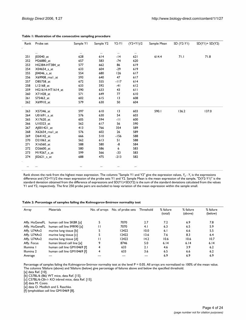
Table 2: Percentage of samples failing the Kolmogorov-Smirnov normality test

Array Materials No. of arrays No. of probe sets Threshold % failure (total)

% failure (above)

% failure (below)

Affy. HuGeneFL human cell line SKBR [a] 5 7070 2.7 7.2 6.9 7.8Affy. HuGeneFL human cell line IMR90 [a] 11 7070 4.1 6.3 6.5 5.9Affy. U74Av2 murine lung tissue [b] 5 12422 10.0 6.1 6.6 5.5Affy. U74Av2 murine lung tissue [c] 5 12422 13.6 7.6 8.3 6.4Affy. U74Av2 murine lung tissue [d] 11 12422 14.2 10.6 10.6 10.7Affy. Focus human blood cell line [e] 9 8746 5.0 6.14 6.14 6.14Illumina 1 human cell line GM10469 [f] 4 633 2.1 4.6 3.9 6.2Illumina 2 human cell line GM10469 [f] 4 633 3.6 6.5 6.6 6.2Average --- --- --- --- 6.9 6.9 6.9

Percentage of samples failing the Kolmogorov-Smirnov normality test at the level P = 0.05. All arrays are normalized to 100% of the mean value. The columns %failure (above) and %failure (below) give percentage of failures above and below the specified threshold.[a] data Ref. [10].[b] C57BL/6 (B6) WT mice, data Ref. [15].[c] C57BL/6-Cftr-/- KO inbred mice, data Ref. [15].[d] data M. Cosio.[e] data O. Modlich and S. Raschke.[f] lymphoblast cell line GM10469 [8].

Table 1: Illustration of the consecutive sampling procedure

Rank Probe set Sample Y1 Sample Y2 Y2-Y1 (Y2+Y1)/2 Sample Mean SD (Y2-Y1) SD(Y1)+ SD(Y2)

... ... ... ... ...251 J03040_at 628 614 -14 621 614.4 71.1 71.8252 M26880_at 657 583 -74 620253 HG384-HT384_at 577 662 86 619254 X04654_s_at 633 604 -29 619255 J04046_s_at 554 680 126 617256 X69908_rna1_at 593 640 47 617257 D85758_at 672 555 -117 614258 L12168_at 633 592 -41 612259 HG1614-HT1614_at 590 633 43 611260 X71428_at 571 649 77 610261 S75463_at 602 615 13 608262 X69910_at 579 630 50 604

263 X57346_at 597 610 13 603 590.1 136.2 137.0264 U01691_s_at 576 630 54 603265 X17620_at 605 594 -11 600266 U10323_at 562 617 56 590267 AJ001421_at 413 766 354 589268 X62654_rna1_at 576 602 26 589269 D64142_at 666 510 -156 588270 D21063_at 562 613 51 588271 X16560_at 588 580 -8 584272 D26600_at 580 586 6 583273 M19267_s_at 599 566 -33 583274 J02621_s_at 688 475 -213 582

... ... ... ... ... ...

Rank shows the rank from the highest mean expression. The columns "Sample Y1 and Y2" give the expression values, Y2 - Y1 is the expressions difference and (Y2+Y1)/2 the mean expression of the probe sets Y1 and Y2. Sample Mean is the mean expression of the sample, "D(Y2-Y1)" is the standard deviation obtained from the difference of expressions and SD(Y1)+SD(Y2) is the sum of the standard deviations calculated from the values Y1 and Y2, respectively. The first 250 probe pairs are excluded to keep variation of the mean expression within the sample small.


close to the mean D in a given range. The figures showquantile-quantile plots (Q-Q plots), comparing theobserved expression values to the corresponding values ofthe inverse normal cumulative distribution. The last panelD shows one sample that failed the test.

Furthermore, we observed that the probe sets with themean expressions within a "reasonably small" range had,on average, a similar variance. Figure 2A shows pooleddata of the 62 probe sets in the expression range from -0.1to 0.1 (cell line IMR90, 11 replicates, Ref. [10]) in Q-Qplot in comparison to the inverse normal cumulative dis-tribution with good agreement except for about six out-liers. The picture changes when we scan probe sets with awide range of mean expressions. Figure 2B shows the Q-Qplot of 185 probes sets in the range of means from 500 to1000; the lower part of the graph deviates substantiallyfrom the straight line. When we plotted the relativeexpression (i.e. expressions of the individual probe setsdivided by the mean of 11 arrays; Figure 2C), we got allthe points, except for about ten outliers, back on the 45°line. This implies that the standard deviation is linearlyproportional to the mean expression level.

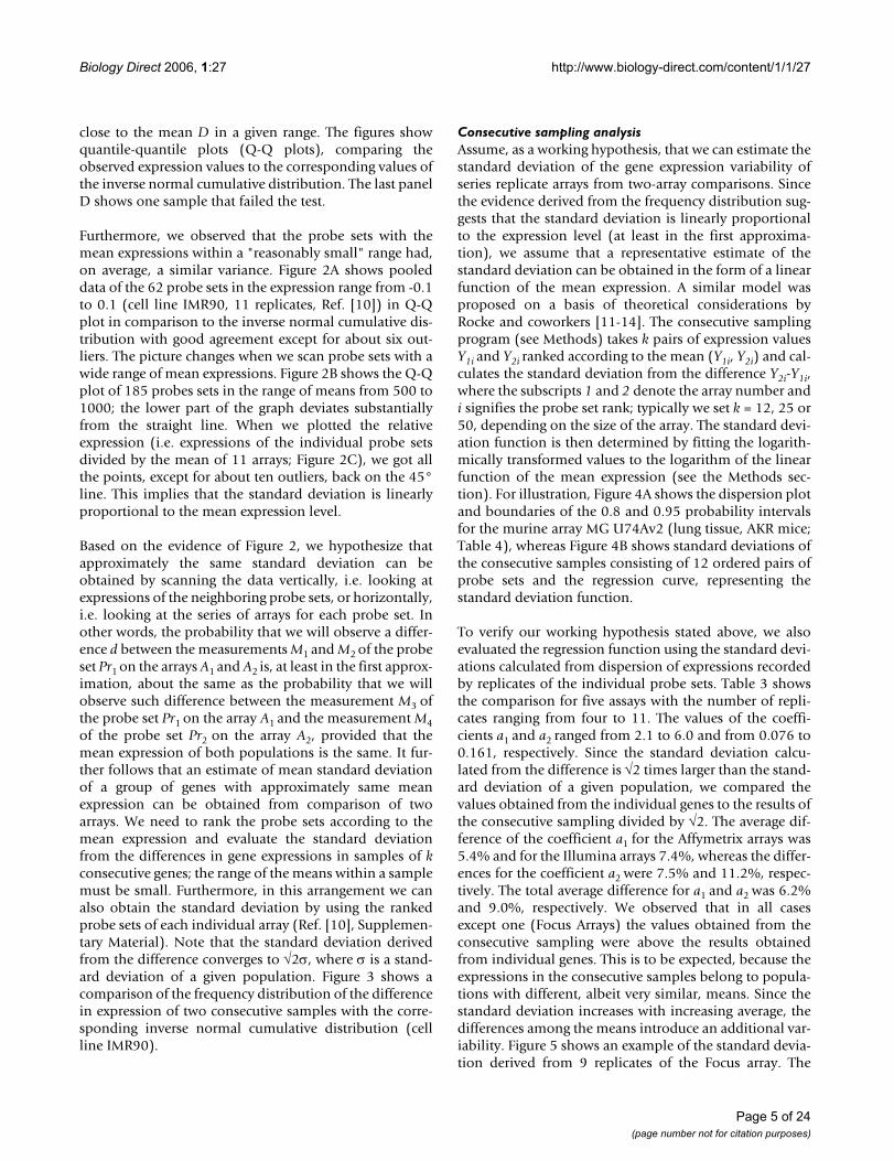
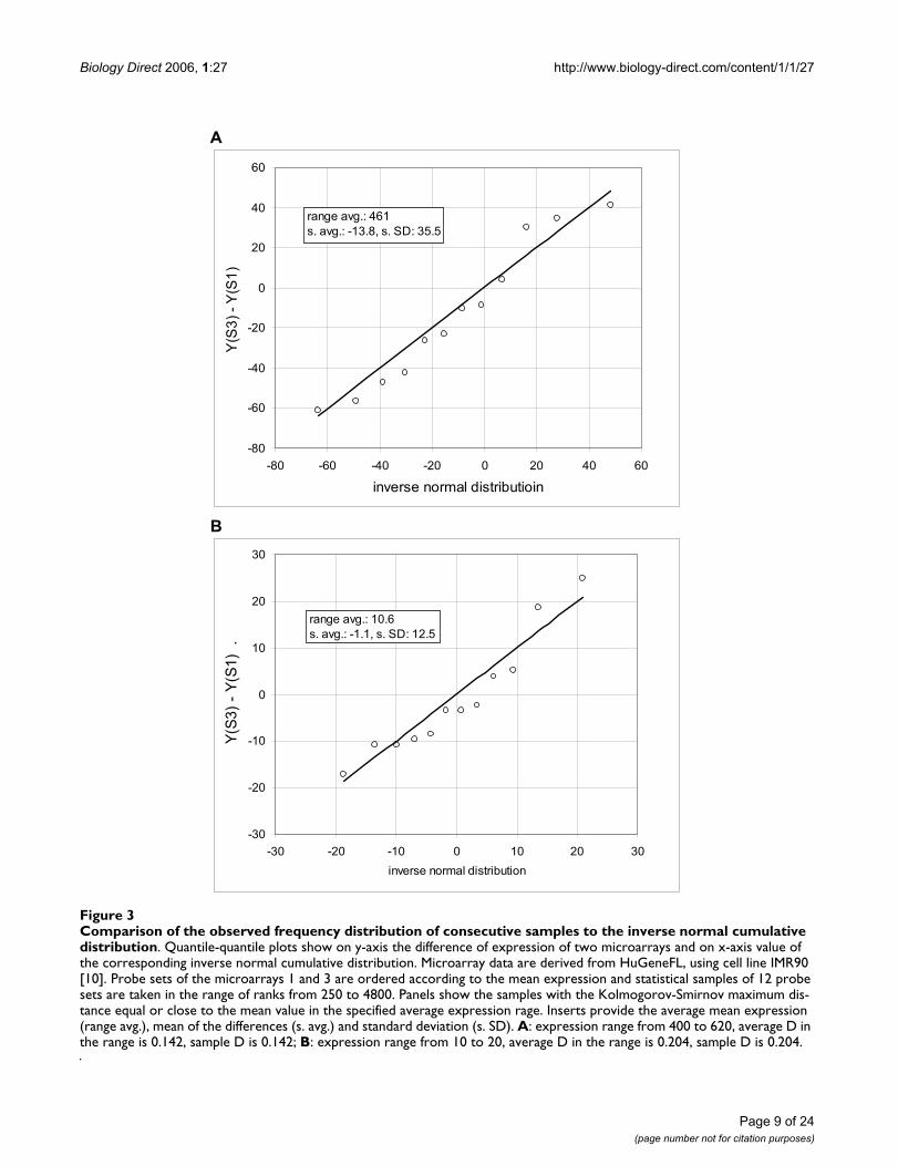
Based on the evidence of Figure 2, we hypothesize thatapproximately the same standard deviation can beobtained by scanning the data vertically, i.e. looking atexpressions of the neighboring probe sets, or horizontally,i.e. looking at the series of arrays for each probe set. Inother words, the probability that we will observe a differ-ence d between the measurements M1 and M2 of the probeset Pr1 on the arrays A1 and A2 is, at least in the first approx-imation, about the same as the probability that we willobserve such difference between the measurement M3 ofthe probe set Pr1 on the array A1 and the measurement M4of the probe set Pr2 on the array A2, provided that themean expression of both populations is the same. It fur-ther follows that an estimate of mean standard deviationof a group of genes with approximately same meanexpression can be obtained from comparison of twoarrays. We need to rank the probe sets according to themean expression and evaluate the standard deviationfrom the differences in gene expressions in samples of kconsecutive genes; the range of the means within a samplemust be small. Furthermore, in this arrangement we canalso obtain the standard deviation by using the rankedprobe sets of each individual array (Ref. [10], Supplemen-tary Material). Note that the standard deviation derivedfrom the difference converges to √2σ, where σ is a stand-ard deviation of a given population. Figure 3 shows acomparison of the frequency distribution of the differencein expression of two consecutive samples with the corre-sponding inverse normal cumulative distribution (cellline IMR90).

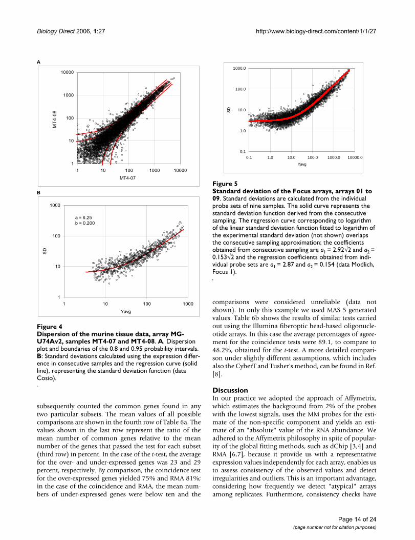
Consecutive sampling analysisAssume, as a working hypothesis, that we can estimate thestandard deviation of the gene expression variability ofseries replicate arrays from two-array comparisons. Sincethe evidence derived from the frequency distribution sug-gests that the standard deviation is linearly proportionalto the expression level (at least in the first approxima-tion), we assume that a representative estimate of thestandard deviation can be obtained in the form of a linearfunction of the mean expression. A similar model wasproposed on a basis of theoretical considerations byRocke and coworkers [11-14]. The consecutive samplingprogram (see Methods) takes k pairs of expression valuesY1i and Y2i ranked according to the mean (Y1i, Y2i) and cal-culates the standard deviation from the difference Y2i-Y1i,where the subscripts 1 and 2 denote the array number andi signifies the probe set rank; typically we set k = 12, 25 or50, depending on the size of the array. The standard devi-ation function is then determined by fitting the logarith-mically transformed values to the logarithm of the linearfunction of the mean expression (see the Methods sec-tion). For illustration, Figure 4A shows the dispersion plotand boundaries of the 0.8 and 0.95 probability intervalsfor the murine array MG U74Av2 (lung tissue, AKR mice;Table 4), whereas Figure 4B shows standard deviations ofthe consecutive samples consisting of 12 ordered pairs ofprobe sets and the regression curve, representing thestandard deviation function.

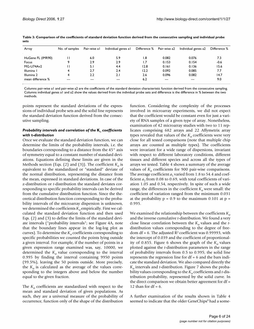
To verify our working hypothesis stated above, we alsoevaluated the regression function using the standard devi-ations calculated from dispersion of expressions recordedby replicates of the individual probe sets. Table 3 showsthe comparison for five assays with the number of repli-cates ranging from four to 11. The values of the coeffi-cients a1 and a2 ranged from 2.1 to 6.0 and from 0.076 to0.161, respectively. Since the standard deviation calcu-lated from the difference is √2 times larger than the stand-ard deviation of a given population, we compared thevalues obtained from the individual genes to the results ofthe consecutive sampling divided by √2. The average dif-ference of the coefficient a1 for the Affymetrix arrays was5.4% and for the Illumina arrays 7.4%, whereas the differ-ences for the coefficient a2 were 7.5% and 11.2%, respec-tively. The total average difference for a1 and a2 was 6.2%and 9.0%, respectively. We observed that in all casesexcept one (Focus Arrays) the values obtained from theconsecutive sampling were above the results obtainedfrom individual genes. This is to be expected, because theexpressions in the consecutive samples belong to popula-tions with different, albeit very similar, means. Since thestandard deviation increases with increasing average, thedifferences among the means introduce an additional var-iability. Figure 5 shows an example of the standard devia-tion derived from 9 replicates of the Focus array. The



points represent the standard deviations of the expres-sions of individual probe sets and the solid line representsthe standard deviation function derived from the consec-utive sampling.

Probability intervals and correlation of the Kα coefficients with t-distributionOnce we evaluate the standard deviation function, we candetermine the limits of the probability intervals, i.e. theboundaries corresponding to a distance from the 45° axisof symmetry equal to a constant number of standard devi-ations. Equations defining these limits are given in theMethods section (Eqs. (2) and (3)). The coefficient Kα isequivalent to the standardized or "standard" deviate ofthe normal distribution, representing the distance fromthe mean, expressed in standard deviations. In case of thez-distribution or t-distribution the standard deviates cor-responding to specific probability intervals can be derivedfrom the cumulative distribution function. Since the the-oretical distribution function corresponding to the proba-bility intervals of the microarray dispersion is unknown,we determined the coefficients Kα empirically. First we cal-culated the standard deviation function and then usedEqs. (2) and (3) to define the limits of the standard devi-ate intervals ("probability intervals"; see Figure 4A, notethat the boundary lines appear in the log-log plot ascurves). To determine the Kα coefficients corresponding tospecific probabilities we counted the points lying outsidea given interval. For example, if the number of points in agiven expression range examined was, say, 10000, wedetermined the Kα value corresponding to the interval0.995 by finding the interval containing 9950 points(99.5%), leaving the 50 points outside. More precisely,the Kα is calculated as the average of the values corre-sponding to the integers above and below the numberequal to the given fraction.

The Kα coefficients are standardized with respect to themean and standard deviation of given populations. Assuch, they are a universal measure of the probability ofoccurrence, function only of the shape of the distribution

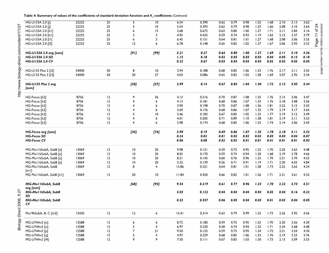
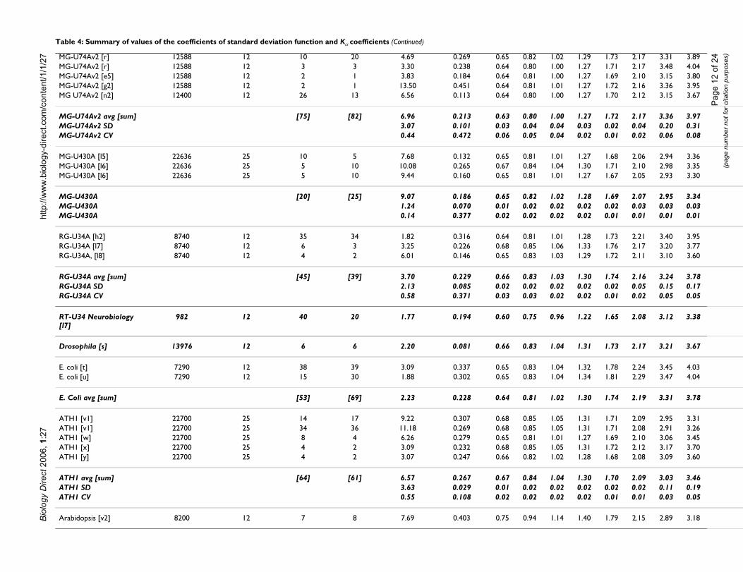
function. Considering the complexity of the processesinvolved in microarray experiments, we did not expectthat the coefficient would be constant even for just a vari-ety of RNA samples of a given type of array. Nonetheless,examination of 42 microarray studies with two to 11 rep-licates comprising 682 arrays and 22 Affymetrix arraytypes revealed that values of the Kα coefficients were veryclose for all tested comparisons (note that multiple chiparrays are counted as multiple types). The coefficientswere invariant for a wide range of dispersions, invariantwith respect to different laboratory conditions, differenttissues and different species and across all the types ofarrays we tested. Table 4 shows a summary of the averagevalues of Kα coefficients for 900 pair-wise comparisons.The average coefficient a1 varied from 1.8 to 54.4 and coef-ficient a2 from 0.08 to 0.69, with total coefficients of vari-ation 1.05 and 0.54, respectively. In spite of such a widerange, the differences in the coefficient Kα were small: thecoefficient of variation ranged from the minimum 0.031at the probability p = 0.9 to the maximum 0.101 at p =0.995.

We examined the relationship between the coefficients Kαand the inverse cumulative t-distribution. We found a veryclose linear correlation between the Kα values and the t-distribution values corresponding to the degree of free-dom df = 6. The adjusted R2 coefficient was 0.99993, withthe intercept of 0.039 and the coefficient of proportional-ity of 0.855. Figure 6 shows the graph of the Kα valuesplotted against the t-distribution parameters in the rangeof probability intervals from 0.5 to 0.995; the solid linerepresents the regression line for df = 6 and the bars indi-cate the standard deviation. We also compared directly theKα intervals and t-distribution. Figure 7 shows the proba-bility values corresponding to the Kα coefficients and t-dis-tribution probability, represented by the solid curve. Inthe direct comparison we obtain better agreement for df =12 than for df = 6.

A further examination of the results shown in Table 4seemed to indicate that the older GeneChips® had a some-

Table 3: Comparison of the coefficients of standard deviation function derived from the consecutive sampling and individual probe sets

Array No. of samples Pair-wise a1 Individual genes a1 Difference % Pair-wise a2 Individual genes a2 Difference %

HuGene FL (IMR90) 11 6.0 5.9 1.8 0.082 0.076 7.3Focus 9 2.9 2.9 1.7 0.153 0.154 -0.6MG-U74Av2 11 5.1 4.4 12.8 0.161 0.136 15.6Illumina 1 4 2.7 2.4 12.2 0.092 0.085 7.7Illumina 2 4 2.2 2.1 2.6 0.096 0.082 14.7mean difference % --- --- --- 6.2 --- --- 9.0

Columns pair-wise a1 and pair-wise a2 are the coefficients of the standard deviation characteristic function derived from the consecutive sampling. Columns individual genes a1 and a2 show the values derived from the individual probe sets and difference is the difference in % between the two methods.



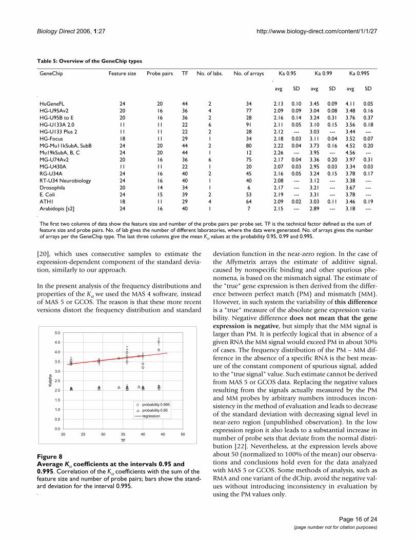
what broader distribution. For example, the mean Kα at0.995 for the array HuGene FL was 4.11, while these val-ues for the later versions HG-U95A and HG-U133A were3.48 and 3.56, respectively. To assess the correlationbetween the developing technology and shape of the Kαdistribution, we need a quantitative parameter, reflectingthe technological advancement. One possibility is the fea-ture size and number of probe pairs per set, which havebeen systematically decreasing with time. Table 5 shows

the overview of the selected Kα values correlated with thetechnical factor TF, defined as the sum of the feature sizeand number of the probe pairs per probe set. In Figure 8we present the Kα values at 0.95 and 0.995, plotted againstTF. The regression line showed a slight decreasing ten-dency of the Kα values at 0.995 with the decreasing TF, butthe graph was not very convincing; the adjusted R2 wasonly 0.31. No trend was discernible at the probability of0.95.

Comparison of the observed frequency distribution to the inverse normal cumulative distributionFigure 1Comparison of the observed frequency distribution to the inverse normal cumulative distribution. Quantile-quantile plots show on y-axis the observed expression and on x-axis value of the corresponding inverse normal cumulative dis-tribution. Microarray data are derived from HuGeneFL, using IMR90 cell line with 11 samples. Panels show the probe sets with the Kolmogorov-Smirnov maximum distance D equal or close to the mean value in the specified average expression rage. Inserts provide the Affymetrix probe set identification, average expression for a given gene and standard deviation. A: probe set HG2279-HT2375_at, rank 43, expression range from 1000 to 6681 (high range, maximum), average D in the range is 0.176, sample D is 0.176; B: probe set Z23091_rna1_at, rank 5484, expression range from -0.4 to 0.4 (near-zero range), average D in the rang is 0.181, sample D is 0.182; C: probe set X95876_at, rank 7003, expression range from -20 to -923 (negative range, minimum), average D in the range is 0.183, sample D is 0.182; D: example of the probe set that failed the test – probe set M14199_s_at, rank 25, sample D is 0.204 (data Novak et al., IMR90 [10]).

A B

1800

1900

2000

2100

2200

2300

1800 1900 2000 2100 2200 2300

inverse normal distribution

obse

rve

d ex

pres

sion

HG2279-HT2375_atavg.: 2012; SD: 147.3

-15

-5

5

15

-15 -5 5 15


obse

rve

d e

xpre

ssio

n

Z23091_rna1_atavg.: -0.3; SD: 6.5

C D

-100

-80

-60

-40

-20

0

20

-100 -80 -60 -40 -20 0 20


ob

serv

ed e

xpre

ssio

n X95876_at

avg.: -41.7; SD: 27.7

1900

2100

2300

2500

2700

2900

2000 2200 2400 2600 2800


obse

rved

exp

ress

ion

M14199_s_atavg.: 2351; SD: 187.4



We found the probability intervals useful for estimatingthe significance of the observed differences, in particularin assays with small numbers of replicates (four or less).The Kα coefficients representing the number of standarddeviates that separates the measured values from the refer-ence mean values provide an objective measure of dissim-ilarity between the populations under consideration. Forthe single normal population the interpretation isstraightforward. However, in case of the microarray datawe deal with the multitude of populations and the theo-retical Kα function is unknown; our correlation resultsthough indicate that a universal function, encompassingall GeneChip® types, exists. We could use the Kα valuesobtained from correlations instead of the theoretical val-ues; however, the experience has shown that the resultsare not reliable. First, considering the large number of val-ues on the arrays even small differences in the Kα functiontranslate into substantial differences in number of candi-dates. Second, quite frequently the unplanned differencesbetween the samples cause deviations from the expectedbehavior and render comparison with the general func-tion unsuitable. Therefore, in practice, we use the Kα coef-ficients only for ranking.

To determine the best candidate genes differentiallyexpressed, we search for the genes with the largest Kα in allor most of the comparisons. We named this method "con-secutive sampling and coincidence test." Briefly, we calcu-late the Kα coefficients in all possible N pair-wisecomparisons and select the probe sets with expressionsbeyond a given probability interval in at least M compar-isons; the upper limit of probability of observing f falsepositives can be calculated theoretically, assuming ran-dom selection. Detailed discussion is beyond the scope ofthis study (a particular example of application to the anal-ysis of five-replicate assay of murine lung tissue can befound in Ref. [15]). The main advantages of this approachare that: 1) it is a nonparametric method; 2) applicable toassays with small number of replicates (as small as two);3) it examines all pair-wise comparisons and makes easyto identify and automatically flag problematic arrays; 4)the probability of false positives can be easily calculatedfrom the binomial distributions or estimated by straight-forward simulations [8]. Here, as a brief illustration of theconsistency of this approach, Table 6a shows the analysisof five replicates of murine GeneChips MG-U74Av2,labeled as mg1 to mg5 (data Ref. [15]). The purpose is toexamine consistency of the results of analysis of differen-tial expression using the t-test, coincidence method andRMA. For the test, we defined five subsets: [mg1, 2, 3, 4],[mg1, 2, 3, 5], [mg1, 2, 4, 5], etc. and selected the candi-date genes. The threshold of selection for the t-test was P= 0.01, for the coincidence 12 out of possible 16 cases,and for the RMA minimum fold difference 2. We selectedthe genes satisfying the given criteria for each subset and

Comparison of the observed frequency distribution to the inverse normal cumulative distribution, pooled dataFigure 2Comparison of the observed frequency distribution to the inverse normal cumulative distribution, pooled data. Quantile-quantile plots show on y-axis the observed expression and on x-axis value of the correspond-ing inverse normal cumulative distribution. Microarray data are derived from HuGeneFL, using the cell line IMR90 with 11 samples, pooled data. A: expression range from -0.1 to 0.1, 62 probe sets; B: expression range from 500 to 1000, 185 probe sets; C: expression range from 500 to 1000, 185 probe sets, relative expression values (sample expression divided by the mean of 11 samples; data Novak et al. [10]).

A

-30

-20

-10

0

10

20

30

-20 -10 0 10 20


observ

ed e

xpre

ssio

n

B

0

200

400

600

800

1000

1200

1400

0 200 400 600 800 1000 1200 1400


ob

se

rve

d e

xp

ressio

n

C

0.0

0.2

0.4

0.6

0.8

1.0

1.2

1.4

1.6

0.6 0.8 1.0 1.2 1.4


observ

ed e

xpre

ssio

n




Comparison of the observed frequency distribution of consecutive samples to the inverse normal cumulative distributionFigure 3Comparison of the observed frequency distribution of consecutive samples to the inverse normal cumulative distribution. Quantile-quantile plots show on y-axis the difference of expression of two microarrays and on x-axis value of the corresponding inverse normal cumulative distribution. Microarray data are derived from HuGeneFL, using cell line IMR90 [10]. Probe sets of the microarrays 1 and 3 are ordered according to the mean expression and statistical samples of 12 probe sets are taken in the range of ranks from 250 to 4800. Panels show the samples with the Kolmogorov-Smirnov maximum dis-tance equal or close to the mean value in the specified average expression rage. Inserts provide the average mean expression (range avg.), mean of the differences (s. avg.) and standard deviation (s. SD). A: expression range from 400 to 620, average D in the range is 0.142, sample D is 0.142; B: expression range from 10 to 20, average D in the range is 0.204, sample D is 0.204.

A

-80

-60

-40

-20

0

20

40

60

-80 -60 -40 -20 0 20 40 60

inverse normal distributioin

Y(S

3)

- Y

(S1

)range avg.: 461

s. avg.: -13.8, s. SD: 35.5

B

-30

-20

-10

0

10

20

30

-30 -20 -10 0 10 20 30


Y(S

3)

- Y

(S1)

.

range avg.: 10.6

s. avg.: -1.1, s. SD: 12.5

of 2

4(p

age

num

ber n

ot fo

r cita

tion

purp

oses

)

a values in given probability intervals

0.800 0.900 0.950 0.990 0.995

1.275 1.711 2.145 3.226 3.7410.045 0.052 0.080 0.270 0.3900.035 0.030 0.037 0.084 0.104

1.27 1.71 2.16 3.41 4.091.24 1.73 2.24 3.58 4.181.20 1.60 2.03 3.39 4.101.18 1.60 2.07 3.42 4.07

1.22 1.66 2.13 3.45 4.110.04 0.07 0.10 0.09 0.050.04 0.04 0.05 0.03 0.01

1.30 1.83 2.32 2.98 3.261.27 1.68 2.07 3.05 3.551.26 1.67 2.07 3.07 3.561.25 1.66 2.07 3.06 3.551.24 1.66 2.04 3.02 3.501.26 1.65 2.05 3.05 3.621.25 1.66 2.04 2.92 3.311.20 1.64 2.10 3.22 3.711.26 1.69 2.09 2.98 3.29

1.26 1.68 2.09 3.04 3.480.03 0.06 0.09 0.08 0.160.02 0.04 0.04 0.03 0.05

1.30 1.80 2.28 3.18 3.681.24 1.65 2.02 3.08 3.541.30 1.77 2.25 3.39 3.981.23 1.62 2.00 3.06 3.611.28 1.77 2.33 3.80 4.421.23 1.62 2.05 2.98 3.481.27 1.78 2.29 3.53 4.081.25 1.64 2.02 2.88 3.31

1.26 1.71 2.16 3.24 3.760.03 0.08 0.14 0.31 0.370.02 0.05 0.07 0.10 0.10

1.28 1.72 2.14 3.14 3.621.31 1.75 2.17 3.18 3.631.32 1.77 2.21 3.26 3.751.26 1.67 2.08 3.05 3.541.27 1.68 2.08 3.04 3.48

Biol

ogy

Dire

ct 2

006,

1:2

7ht

tp://

ww

w.b

iolo

gy-d

irect

.com

/con

tent

/1/1

/27

Table 4: Summary of values of the coefficients of standard deviation function and Kα coefficients

GeneChip/average/SD/CV No. of probe sets Cons. samp. size No. of arrays No. of comp. Coefficient. of st. dev. function Average Kalph

a1 a2 0.500 0.600 0.700

Total average [sum] [682] [900] 9.66 0.266 0.642 0.808 1.009Total SD 9.99 0.146 0.033 0.039 0.043Total CV 1.03 0.550 0.052 0.049 0.043

HuGeneFL [a1] 7070 12 11 54 8.61 0.115 0.64 0.81 1.01HuGeneFL [b] 7070 12 13 78 8.09 0.418 0.61 0.77 0.97HuGeneFL [c] 7070 25 5 10 34.58 0.435 0.61 0.76 0.94HuGeneFL [c] 7070 25 5 10 28.93 0.393 0.59 0.73 0.92

HuGeneFL avg [sum] [34] [152] 20.05 0.34 0.61 0.77 0.96HuGeneFL SD 13.71 0.15 0.02 0.03 0.04HuGeneFL CV 0.68 0.44 0.04 0.04 0.04

HG-U95Av2 [d] 12559 12 5 10 6.30 0.688 0.61 0.78 1.00HG-U95Av2 [e1] 12559 25 15 15 10.49 0.199 0.65 0.82 1.01HG-U95Av2 [e2] 12559 25 15 15 10.59 0.200 0.64 0.81 1.01HG-U95Av2 [e3] 12559 25 15 15 10.41 0.189 0.63 0.80 1.00HG-U95Av2 [e4] 12559 25 12 12 10.91 0.185 0.63 0.79 0.99HG-U95Av2 [e5] 12559 25 4 2 6.50 0.394 0.65 0.82 1.01HG-U95Av2 [f] 12559 25 4 2 5.64 0.155 0.64 0.81 1.00HG-U95Av2 [g1] 12559 25 2 1 4.79 0.479 0.61 0.76 0.95HG-U95Av2 [g1] 12559 25 5 10 3.31 0.500 0.64 0.80 1.00

HG-U95Av2 avg [sum] [77] [82] 7.66 0.33 0.63 0.80 1.00HG-U95Av2 SD 2.94 0.19 0.02 0.02 0.02HG-U95Av2 CV 0.38 0.57 0.02 0.02 0.02

HG-U95B [d] 12563 12 5 10 16.26 0.636 0.63 0.80 1.01HG-U95B [e5] 12563 25 2 1 17.95 0.167 0.64 0.80 0.99HG-U95C [d] 12587 12 5 10 20.57 0.603 0.64 0.81 1.02HG-U95C [e5] 12587 25 2 1 16.42 0.178 0.63 0.79 0.99HG-U95D [d] 12587 12 5 10 39.79 0.501 0.62 0.78 0.99HG-U95D [e5] 12587 25 2 1 54.45 0.240 0.63 0.79 0.99HG-U95E [d] 12582 12 5 10 31.84 0.534 0.60 0.76 0.97HG-U95E [e5] 12582 25 2 1 45.64 0.215 0.63 0.79 1.00

HG-U95B to E avg [sum] [28] [44] 30.37 0.38 0.63 0.79 0.99HG-U95B to E SD 14.87 0.20 0.01 0.01 0.02HG-U95B to E CV 0.49 0.53 0.02 0.02 0.02

HG-U133A 2.0 [e6] 22225 25 15 15 4.55 0.091 0.65 0.82 1.02HG-U133A 2.0 [e7] 22225 25 15 15 4.50 0.106 0.66 0.84 1.04HG-U133A 2.0 [e8] 22225 25 12 12 4.10 0.108 0.67 0.84 1.05HG-U133A 2.0 [h1] 22225 25 8 4 3.91 0.288 0.64 0.80 1.00HG-U133A 2.0 [i1] 22225 12 4 6 6.25 0.210 0.65 0.82 1.01

of 2

4(p

age

num

ber n

ot fo

r cita

tion

purp

oses

)1.25 1.68 2.10 3.13 3.621.25 1.66 2.08 3.10 3.641.27 1.71 2.11 2.84 3.161.19 1.65 2.15 3.37 3.791.27 1.68 2.08 3.06 3.551.27 1.67 2.06 2.93 3.33

1.27 1.69 2.11 3.10 3.560.03 0.04 0.05 0.15 0.180.03 0.02 0.02 0.05 0.05

1.33 1.76 2.17 3.11 3.551.28 1.69 2.07 2.95 3.34

1.30 1.72 2.12 3.03 3.44

1.35 1.76 2.15 3.06 3.471.33 1.76 2.18 3.08 3.561.36 1.81 2.22 3.15 3.551.35 1.79 2.19 3.17 3.641.33 1.77 2.19 3.12 3.491.38 1.81 2.19 3.11 3.531.32 1.74 2.14 3.06 3.43

1.35 1.78 2.18 3.11 3.520.02 0.03 0.03 0.04 0.070.01 0.01 0.01 0.01 0.02

1.22 1.70 2.20 3.65 4.481.20 1.68 2.19 3.78 4.661.23 1.70 2.21 3.70 4.521.19 1.71 2.30 4.03 4.841.28 1.73 2.22 3.62 4.24

1.26 1.71 2.21 3.61 4.32

1.23 1.70 2.22 3.73 4.51

0.04 0.02 0.04 0.16 0.22

0.03 0.01 0.02 0.04 0.05

1.25 1.73 2.26 3.95 4.56

1.23 1.70 2.20 3.56 4.301.23 1.71 2.24 3.68 4.481.24 1.72 2.21 3.54 4.301.33 1.76 2.19 3.23 3.761.30 1.73 2.13 3.09 3.53

Biol

ogy

Dire

ct 2

006,

1:2

7ht

tp://

ww

w.b

iolo

gy-d

irect

.com

/con

tent

/1/1

/27 HG-U133A 2.0 [j] 22225 25 5 10 6.54 0.390 0.62 0.79 0.98

HG-U133A 2.0 [j] 22225 25 5 10 5.54 0.393 0.62 0.79 0.98HG-U133A 2.0 [k1] 22225 25 6 15 3.68 0.672 0.63 0.80 1.00HG-U133A 2.0 [k1] 22225 25 3 3 4.95 0.435 0.59 0.74 0.93HG-U133A 2.0 [l1] 22225 25 6 3 6.45 0.151 0.64 0.81 1.01HG-U133A 2.0 [l2] 22225 25 12 6 6.78 0.148 0.65 0.82 1.02

HG-U133A 2.0 avg [sum] [91] [99] 5.21 0.27 0.64 0.80 1.00HG-U133A 2.0 SD 1.15 0.18 0.02 0.03 0.03HG-U133A 2.0 CV 0.22 0.67 0.03 0.03 0.03

HG-U133 Plus 2 [i2] 54000 50 8 10 3.94 0.188 0.68 0.85 1.06HG-U133 Plus 2 [l3] 54000 50 20 27 4.03 0.086 0.65 0.82 1.02

HG-U133 Plus 2 avg [sum]

[28] [37] 3.99 0.14 0.67 0.83 1.04

HG-Focus [k2] 8756 12 9 36 4.13 0.216 0.70 0.87 1.08HG-Focus [k2] 8756 12 4 6 4.13 0.181 0.68 0.86 1.07HG-Focus [k2] 8756 12 4 6 3.90 0.198 0.70 0.87 1.08HG-Focus [k2] 8756 12 4 6 3.69 0.176 0.68 0.86 1.07HG-Focus [k2] 8756 12 5 10 3.46 0.183 0.67 0.85 1.05HG-Focus [k2] 8756 12 4 6 4.01 0.205 0.71 0.89 1.10HG-Focus [k2] 8756 12 4 6 3.98 0.174 0.68 0.85 1.06

HG-Focus avg [sum] [34] [76] 3.90 0.19 0.69 0.86 1.07HG-Focus SD 0.24 0.02 0.01 0.02 0.02HG-Focus CV 0.06 0.08 0.02 0.02 0.01

MG-Mu11kSubA, SubB [a] 13069 12 10 20 9.98 0.121 0.59 0.75 0.95MG-Mu11kSubA, SubB [a] 13069 12 10 20 8.03 0.170 0.59 0.74 0.94MG-Mu11kSubA, SubB [a] 13069 12 10 20 8.21 0.145 0.60 0.76 0.96MG-Mu11kSubA, SubB [a] 13069 12 10 20 5.32 0.139 0.56 0.71 0.91MG-Mu11kSubA, SubB [m1]

13069 12 8 4 13.86 0.321 0.64 0.81 1.01

MG Mu11kSubA, SubB [n1] 13069 12 20 10 11.84 0.420 0.66 0.82 1.01

MG-Mu11kSubA, SubB avg [sum]

[68] [94] 9.54 0.219 0.61 0.77 0.96

MG-Mu11kSubA, SubB SD

3.03 0.122 0.04 0.04 0.04

MG-Mu11kSubA, SubB CV

0.32 0.557 0.06 0.05 0.04

Mu19kSubA, B, C [m2] 12420 12 12 6 15.41 0.314 0.63 0.79 0.99

MG-U74Av2 [o] 12588 12 6 6 8.72 0.180 0.59 0.75 0.95MG-U74Av2 [o] 12588 12 5 4 6.97 0.230 0.58 0.74 0.94MG-U74Av2 [p] 12588 12 7 21 9.50 0.125 0.59 0.75 0.95MG-U74Av2 [q] 12588 12 5 4 4.97 0.229 0.68 0.85 1.06MG-U74Av2 [l4] 12588 12 9 9 7.50 0.111 0.67 0.83 1.03

Table 4: Summary of values of the coefficients of standard deviation function and Kα coefficients (Continued)

of 2

4(p

age

num

ber n

ot fo

r cita

tion

purp

oses

)1.29 1.73 2.17 3.31 3.891.27 1.71 2.17 3.48 4.041.27 1.69 2.10 3.15 3.801.27 1.72 2.16 3.36 3.951.27 1.70 2.12 3.15 3.67

1.27 1.72 2.17 3.36 3.970.03 0.02 0.04 0.20 0.310.02 0.01 0.02 0.06 0.08

1.27 1.68 2.06 2.94 3.361.30 1.71 2.10 2.98 3.351.27 1.67 2.05 2.93 3.30

1.28 1.69 2.07 2.95 3.340.02 0.02 0.03 0.03 0.030.02 0.01 0.01 0.01 0.01

1.28 1.73 2.21 3.40 3.951.33 1.76 2.17 3.20 3.771.29 1.72 2.11 3.10 3.60

1.30 1.74 2.16 3.24 3.780.02 0.02 0.05 0.15 0.170.02 0.01 0.02 0.05 0.05

1.22 1.65 2.08 3.12 3.38

1.31 1.73 2.17 3.21 3.67

1.32 1.78 2.24 3.45 4.031.34 1.81 2.29 3.47 4.04

1.30 1.74 2.19 3.31 3.78

1.31 1.71 2.09 2.95 3.311.31 1.71 2.08 2.91 3.261.27 1.69 2.10 3.06 3.451.31 1.72 2.12 3.17 3.701.28 1.68 2.08 3.09 3.60

1.30 1.70 2.09 3.03 3.460.02 0.02 0.02 0.11 0.190.02 0.01 0.01 0.03 0.05

1.40 1.79 2.15 2.89 3.18
Biol
ogy

Dire

ct 2

006,

1:2

7ht

tp://

ww

w.b

iolo

gy-d

irect

.com

/con

tent

/1/1

/27 MG-U74Av2 [r] 12588 12 10 20 4.69 0.269 0.65 0.82 1.02

MG-U74Av2 [r] 12588 12 3 3 3.30 0.238 0.64 0.80 1.00MG-U74Av2 [e5] 12588 12 2 1 3.83 0.184 0.64 0.81 1.00MG-U74Av2 [g2] 12588 12 2 1 13.50 0.451 0.64 0.81 1.01MG U74Av2 [n2] 12400 12 26 13 6.56 0.113 0.64 0.80 1.00

MG-U74Av2 avg [sum] [75] [82] 6.96 0.213 0.63 0.80 1.00MG-U74Av2 SD 3.07 0.101 0.03 0.04 0.04MG-U74Av2 CV 0.44 0.472 0.06 0.05 0.04

MG-U430A [l5] 22636 25 10 5 7.68 0.132 0.65 0.81 1.01MG-U430A [l6] 22636 25 5 10 10.08 0.265 0.67 0.84 1.04MG-U430A [l6] 22636 25 5 10 9.44 0.160 0.65 0.81 1.01

MG-U430A [20] [25] 9.07 0.186 0.65 0.82 1.02MG-U430A 1.24 0.070 0.01 0.02 0.02MG-U430A 0.14 0.377 0.02 0.02 0.02

RG-U34A [h2] 8740 12 35 34 1.82 0.316 0.64 0.81 1.01RG-U34A [l7] 8740 12 6 3 3.25 0.226 0.68 0.85 1.06RG-U34A, [l8] 8740 12 4 2 6.01 0.146 0.65 0.83 1.03

RG-U34A avg [sum] [45] [39] 3.70 0.229 0.66 0.83 1.03RG-U34A SD 2.13 0.085 0.02 0.02 0.02RG-U34A CV 0.58 0.371 0.03 0.03 0.02

RT-U34 Neurobiology [l7]

982 12 40 20 1.77 0.194 0.60 0.75 0.96

Drosophila [s] 13976 12 6 6 2.20 0.081 0.66 0.83 1.04

E. coli [t] 7290 12 38 39 3.09 0.337 0.65 0.83 1.04E. coli [u] 7290 12 15 30 1.88 0.302 0.65 0.83 1.04

E. Coli avg [sum] [53] [69] 2.23 0.228 0.64 0.81 1.02

ATH1 [v1] 22700 25 14 17 9.22 0.307 0.68 0.85 1.05ATH1 [v1] 22700 25 34 36 11.18 0.269 0.68 0.85 1.05ATH1 [w] 22700 25 8 4 6.26 0.279 0.65 0.81 1.01ATH1 [x] 22700 25 4 2 3.09 0.232 0.68 0.85 1.05ATH1 [y] 22700 25 4 2 3.07 0.247 0.66 0.82 1.02

ATH1 avg [sum] [64] [61] 6.57 0.267 0.67 0.84 1.04ATH1 SD 3.63 0.029 0.01 0.02 0.02ATH1 CV 0.55 0.108 0.02 0.02 0.02

Arabidopsis [v2] 8200 12 7 8 7.69 0.403 0.75 0.94 1.14


Biol

ogy

Dire

ct 2

006,

1:2

7ht

tp://

ww

w.b

iolo

gy-d

irect

.com

/con

tent

/1/1

/27

Page

13

of 2

4(p

age

num

ber n

ot fo

r cita

tion

purp

oses

)

rays is a number of arrays tested, No. of comp. is the cient determining probability interval; "h." stands for (CV) of each GeneChip type are printed in bold italics.

different concentrations.

e; [49] and unpublished data.

No. of probe sets is approximate number of the probe sets on array, Cons. samp. size is number of the probe pairs in a consecutive sample, No. of arnumber of pair-wise comparisons among the replicates, coefficients a1 and a2 are the coefficients of standard deviation function and Kalpha is the coeffi"human," "m." for "murine." Average values, sum of arrays and comparisons (in square brackets), standard deviations (SD) and coefficients of variation Data sources:a1 – J. P. Novak et al., HuGeneFl, IMR90 human cell line [10].a2 – J. P. Novak et al., HuGeneFl, mouse tissues, adult male C57BL/6 [10].b – A.-M. Mes-Masson, P. Tonin and coworkers, HuGeneFL, normal ovarian surface epithelial (NOSE) primary cell cultures, private communication.c – P. Permana, HuGeneFL, human skeletal muscle tissue [35].d – P. Tonin and A.-M. Mes-Masson and coworkers, HG-U95A to E, epithelial ovarian cancer (EOC) cell line [36].e1 – Affymetrix, HG-U95A, latin square, experiments 1 to 5.e2 – Affymetrix, HG-U95A, latin square, experiments 6 to 10.e3 – Affymetrix, HG-U95A, latin square experiments 11 to 15.e4 – Affymetrix, HG-U95A, latin square, experiments 16 to 19.e5 – Affymetrix, HG-U95A to E, Demo Data.e6 – Affymetrix, HG-U133A, latin square, experiments 1 to 5.e7 – Affymetrix, HG-U133A, latin square, experiments 6 to 10.e8 – Affymetrix, HG-U133A, latin square, experiments 11 to 14.f – M. S. Rolph, HG-U95Av2, primary human bronchial epithelial cells.g1 – Z. Gatalica, HG-U95Av2, breast tumor tissues and normal breast tissue samples [37].g2 – Z. Gatalica, MG-U74Av2, mouse kidney tissue.h1 – M. Boerma, HG-U133A 2.0, primary human umbilical vein endothelial cells (HUVECs) and the immortalized HUVEC cell line EA.hy926 [38].h2 – M. Boerma, RG-U34A, cultures enriched for neonatal rat cardiac myocytes or fibroblasts [39].i1 – M. Hajduch, HG-U133A 2.0.i2 – M. Hajduch, HG-U133 plus 2.j – S. Y. Kim and D. J. Volsky, HG-U133A 2.0, human fetal astrocytes, normal and pseudotyped HIV-1 infected [40].k1 – O. Modlich, HG-U133A 2.0, human superficial and invasive bladder tumors [41].k2 – O. Modlich and Raschke, Focus arrays, human lymphoma cell line Kaspas-422, DSMZ no.: ACC 32 (follicular B cell).l1 – C. Wang and J. Xu, HG-U133A 2.0, human lymphoblast cell line.l2 – C. Wang and J. Xu, HG-U133A 2.0, human pancreatic islet.l3 – C. Wang and J. Xu, HG-U133 Plus 2, Stratagene Universal Human Reference RNA, Ambion Human Brain Reference RNA and mixtures of both inl4 – C. Wang and J. Xu, MG-U74Av2, mouse biliary epithelial cells.l5 – C. Wang and J. Xu, MG-U430A, mouse spleen.l6 – C. Wang and J. Xu, MG-U430A, myofibroblast cell line.l7 – C. Wang and J. Xu, RG-U34A, rat livers.l8 – C. Wang and J. Xu, RG-U34A, rat bone marrow stem cells.m1 – McInnes and coworkers, MG-Mu11kSubA, SubB, retinal RNA samples from WT and Rom1 knock-out mice [36].m2 – McInnes, Szego and coworkers, MG-Mu19kSubA, SubB, SubC, retinal RNA samples from WT and Rom1 knock-out mice [42].n1 – Burton, McGehee and coworkers, MG-Mu11kSubA, SubB, 3T3-L1 adipocytes [43].n2 – Burton, McGehee and coworkers, MG-U74Av2,3T3-L1 adipocyte cultures [44].o – M. Cosio, MG-U74Av2, lung tissues, murine strains NZW and AKR.p – R. St-Arnaud, MG-U74Av2, C2C12 cells [45].q – J. Hidalgo, MG-U74Av2, cortex samples, C57B6 normal and IL6 KO mice [46].r – D. Radzioch, C. Guilbault and coworkers, MG-U74Av2, C57BL/6 (B6) WT and C57BL/6-Cftr-/- (KO) inbred mice [15].s – S. E. Choe, Drosophila, Drosophila Gene Collection release 1.0 cDNA clones [19].t – F. Blattner, E. coli antisense genome, E. coli K-12 strain MG1655 and an isogenic fnr::Spr Smr strain [47].u – J. Slonczewski and S. BonDurant, E. coli antisense genome, E. coli K-12 strain W3110 [48].v1 – E. Blumwald and J. Sottosanto, ATH1, A. thaliana ecotype Wassilewskija, wild-type line (WS), nhx1 'knockout' line, and a knockout restoration linv2 – E. Blumwald and J. Sottosanto, arabidopsis, A. thaliana ecotype Wassilewskija, wild-type line (WS), and a nhx1 'knockout' line (unpublished data).w – D. Honys and D. Twell, ATH1, Arabidopsis thaliana ecotype Landsberg erecta plants [50].x – E. Nambara and K. Nakabayashi, ATH1, Arabidopsis thaliana (L.) Heynh of ecotype Columbia [51].y – E. Nambara and K. Tatematsu, ATH1, Arabidopsis thaliana (L.) Heynh of ecotype Columbia [52].



subsequently counted the common genes found in anytwo particular subsets. The mean values of all possiblecomparisons are shown in the fourth row of Table 6a. Thevalues shown in the last row represent the ratio of themean number of common genes relative to the meannumber of the genes that passed the test for each subset(third row) in percent. In the case of the t-test, the averagefor the over- and under-expressed genes was 23 and 29percent, respectively. By comparison, the coincidence testfor the over-expressed genes yielded 75% and RMA 81%;in the case of the coincidence and RMA, the mean num-bers of under-expressed genes were below ten and the

comparisons were considered unreliable (data notshown). In only this example we used MAS 5 generatedvalues. Table 6b shows the results of similar tests carriedout using the Illumina fiberoptic bead-based oligonucle-otide arrays. In this case the average percentages of agree-ment for the coincidence tests were 89.1, to compare to48.2%, obtained for the t-test. A more detailed compari-son under slightly different assumptions, which includesalso the CyberT and Tusher's method, can be found in Ref.[8].

DiscussionIn our practice we adopted the approach of Affymetrix,which estimates the background from 2% of the probeswith the lowest signals, uses the MM probes for the esti-mate of the non-specific component and yields an esti-mate of an "absolute" value of the RNA abundance. Weadhered to the Affymetrix philosophy in spite of popular-ity of the global fitting methods, such as dChip [3,4] andRMA [6,7], because it provide us with a representativeexpression values independently for each array, enables usto assess consistency of the observed values and detectirregularities and outliers. This is an important advantage,considering how frequently we detect "atypical" arraysamong replicates. Furthermore, consistency checks have

Standard deviation of the Focus arrays, arrays 01 to 09Figure 5Standard deviation of the Focus arrays, arrays 01 to 09. Standard deviations are calculated from the individual probe sets of nine samples. The solid curve represents the standard deviation function derived from the consecutive sampling. The regression curve corresponding to logarithm of the linear standard deviation function fitted to logarithm of the experimental standard deviation (not shown) overlaps the consecutive sampling approximation; the coefficients obtained from consecutive sampling are a1 = 2.92√2 and a2 = 0.153√2 and the regression coefficients obtained from indi-vidual probe sets are a1 = 2.87 and a2 = 0.154 (data Modlich, Focus 1).

0.1

1.0

10.0

100.0

1000.0

0.1 1.0 10.0 100.0 1000.0 10000.0

Yavg

SD

Dispersion of the murine tissue data, array MG-U74Av2, samples MT4-07 and MT4-08Figure 4Dispersion of the murine tissue data, array MG-U74Av2, samples MT4-07 and MT4-08. A. Dispersion plot and boundaries of the 0.8 and 0.95 probability intervals. B: Standard deviations calculated using the expression differ-ence in consecutive samples and the regression curve (solid line), representing the standard deviation function (data Cosio).

A

1

10

100

1000

10000

1 10 100 1000 10000

MT4-07

MT

4-0

8.

B

1

10

100

1000

1 10 100 1000

Yavg

SD

a = 6.25

b = 0.200



shown similar rates of coincidence for both RMA andcoincidence testing (Table 6a).

Results of the published studies comparing various meth-ods of analysis are inconsistent and do not provide a clearguidance for selection of the method. Irizarry et al. [7],e.g., reported better detection of differentially expressedgenes by RMA as compared to the dChip [4] and Affyme-trix "Average Difference" (MAS 4) and MAS5 methods.Similarly, Barash et al. rated RMA as the best of the threewith dChip performing slightly better than MAS5 [16].Shedden et al. [17] claim superior results for dChip and"trimmed mean" and inferior results for MAS5 and oneversion of RMA (GCRMA-EB); the other version of RMA(CGRMA-MLE; Wu Z, Irizarry R, Gentleman R, Murillo F,Spencer F., 2003, A Model Based Background Adjustmentfor Oligonucleotide Expression Arrays, Technical Report,John Hopkins University, Department of BiostatisticsWorking Papers, Baltimore, MD) produced mixed results(in trimmed mean the PM-MM differences are ordered,20% of the highest and lowest values are deleted and themean of the remaining probe pairs represents a measureof gene expression). Han et al. [18] compared the Affyme-trix MAS 5, dChip using PM-MM and PM only input andRMA. In this study the PM only variant of dChip and RMAshowed the best performance. The authors also noted thatthe coefficient of variation in replicate experiments in thecase of MAS 5 increases with a decreasing mean signal, butremains approximately constant for PM only of dChipand RMA. Invariance of the coefficient of variation raisesa certain concern: percentage of contribution of the non-specific signal increases with the decreasing concentrationand one would expect that at low concentrations it wouldbe harder to separate it from the specific component.Choe et al. [19] compared various combinations of the sixsteps in the differential expression analysis: backgroundsubtraction, probe-level normalization, PM adjustment(correction for the non-specific signal), expression sum-mary (derivation of the representative gene expressionfrom the multiple probe signals), probe set-level normal-ization and statistical evaluation. This was a particularlyinteresting comparative study, since their experimentaldesign was much closer to real conditions than spiked setsof arrays used in other publications. The authors reportthat the combination of the MAS5 for background correc-tion and PM adjustment, median Polish method or, mar-ginally inferior, MAS5 for expression summary, loess fornormalization and CyberT for statistical evaluation [20]yielded the best results. They also emphasized that, undertheir particular conditions, MM signals provided the bestestimate of the non-specific component. Furthermore,they concluded that in the statistical evaluation it isimportant to account for variation of the standard devia-tion with the mean expression (see also [21]). Theyadopted the CyberT model proposed by Baldi and Lang

Comparison of the Kα distribution and inverse t-distributionFigure 7Comparison of the Kα distribution and inverse t-dis-tribution. Kα values correspond to probabilities from 0.5 to 0.995. The degree of freedom for the inverse t-distribution (solid lines) is 6 and 12.

0.0

0.1

0.2

0.3

0.4

0.5

0.6

0 1 2 3 4 5

Kalpha, t-distribution

pro

ba

bili

ty

Kalpha

df = 12

df = 6

Correlation of the Kα coefficients and inverse t-distributionFigure 6Correlation of the Kα coefficients and inverse t-distri-bution. Figure shows the values of Kα coefficient correlated with the corresponding values of the t-distribution in the range of probabilities from 0.5 to 0.995. The adjusted R2

coefficient is 0.99993, intercept is 0.039 and the coefficient of proportionality is 0.855. The degree of freedom for the t-dis-tribution is 6.

0.0

0.5

1.0

1.5

2.0

2.5

3.0

3.5

4.0

4.5

0 1 2 3 4 5 6

t-distribution

Kalp

ha

df = 5

df = 6

df = 7

regression



[20], which uses consecutive samples to estimate theexpression-dependent component of the standard devia-tion, similarly to our approach.

In the present analysis of the frequency distributions andproperties of the Kα we used the MAS 4 software, insteadof MAS 5 or GCOS. The reason is that these more recentversions distort the frequency distribution and standard

deviation function in the near-zero region. In the case ofthe Affymetrix arrays the estimate of additive signal,caused by nonspecific binding and other spurious phe-nomena, is based on the mismatch signal. The estimate ofthe "true" gene expression is then derived from the differ-ence between perfect match (PM) and mismatch (MM).However, in such system the variability of this differenceis a "true" measure of the absolute gene expression varia-bility. Negative difference does not mean that the geneexpression is negative, but simply that the MM signal islarger than PM. It is perfectly logical that in absence of agiven RNA the MM signal would exceed PM in about 50%of cases. The frequency distribution of the PM – MM dif-ference in the absence of a specific RNA is the best meas-ure of the constant component of spurious signal, addedto the "true signal" value. Such estimate cannot be derivedfrom MAS 5 or GCOS data. Replacing the negative valuesresulting from the signals actually measured by the PMand MM probes by arbitrary numbers introduces incon-sistency in the method of evaluation and leads to decreaseof the standard deviation with decreasing signal level innear-zero region (unpublished observation). In the lowexpression region it also leads to a substantial increase innumber of probe sets that deviate from the normal distri-bution [22]. Nevertheless, at the expression levels aboveabout 50 (normalized to 100% of the mean) our observa-tions and conclusions hold even for the data analyzedwith MAS 5 or GCOS. Some methods of analysis, such asRMA and one variant of the dChip, avoid the negative val-ues without introducing inconsistency in evaluation byusing the PM values only.

Average Kα coefficients at the intervals 0.95 and 0.995Figure 8Average Kα coefficients at the intervals 0.95 and 0.995. Correlation of the Kα coefficients with the sum of the feature size and number of probe pairs; bars show the stand-ard deviation for the interval 0.995.

0.0

0.5

1.0

1.5

2.0

2.5

3.0

3.5

4.0

4.5

5.0

20 25 30 35 40 45 50

TF

Kalp

ha

probability 0.995

probability 0.95

regression

Table 5: Overview of the GeneChip types

GeneChip Feature size Probe pairs TF No. of labs. No. of arrays Ka 0.95 Ka 0.99 Ka 0.995

avg SD avg SD avg SD

HuGeneFL 24 20 44 2 34 2.13 0.10 3.45 0.09 4.11 0.05HG-U95Av2 20 16 36 4 77 2.09 0.09 3.04 0.08 3.48 0.16HG-U95B to E 20 16 36 2 28 2.16 0.14 3.24 0.31 3.76 0.37HG-U133A 2.0 11 11 22 6 91 2.11 0.05 3.10 0.15 3.56 0.18HG-U133 Plus 2 11 11 22 2 28 2.12 --- 3.03 --- 3.44 ---HG-Focus 18 11 29 1 34 2.18 0.03 3.11 0.04 3.52 0.07MG-Mu11kSubA, SubB 24 20 44 2 80 2.22 0.04 3.73 0.16 4.52 0.20Mu19kSubA, B, C 24 20 44 1 12 2.26 --- 3.95 --- 4.56 ---MG-U74Av2 20 16 36 6 75 2.17 0.04 3.36 0.20 3.97 0.31MG-U430A 11 11 22 1 20 2.07 0.03 2.95 0.03 3.34 0.03RG-U34A 24 16 40 2 45 2.16 0.05 3.24 0.15 3.78 0.17RT-U34 Neurobiology 24 16 40 1 40 2.08 --- 3.12 --- 3.38 ---Drosophila 20 14 34 1 6 2.17 --- 3.21 --- 3.67 ---E. Coli 24 15 39 2 53 2.19 --- 3.31 --- 3.78 ---ATH1 18 11 29 4 64 2.09 0.02 3.03 0.11 3.46 0.19Arabidopis [s2] 24 16 40 1 7 2.15 --- 2.89 --- 3.18 ---

The first two columns of data show the feature size and number of the probe pairs per probe set. TF is the technical factor defined as the sum of feature size and probe pairs. No. of lab gives the number of different laboratories, where the data were generated. No. of arrays gives the number of arrays per the GeneChip type. The last three columns give the mean Kα values at the probability 0.95, 0.99 and 0.995.



In the preceding section, we demonstrated that the fre-quency distribution of the random and pseudo-randomfluctuations of microarray data is predominantly normal.The normal frequency distribution is a useful property,allowing straightforward identification of outliers, a con-venient quality check and simple characterization of theobserved data. Normality of the error term is an importantassumption of various global models used for the analysisof measured probe signals, such as dChip [3,4], RMA [5-7] and other approaches [23-25]. Among these onlyPavelka et al. [25] demonstrated that the assumption isjustified. Normality is also a necessary condition for appli-cation of the parametric methods. Here we observed thaton average over 5% of samples deviate from the normaldistribution (using the test threshold of 0.05). It is agreedthat the t-test and ANOVA are rather robust with respect tonormality (e.g. SigmaStat software [SPSS inc.] uses forANOVA the threshold of 0.01), nonetheless the noteddeviations call for caution when using parametric meth-ods, in particular considering that every analysis involvesmultiple testing. Our conclusion differs from that ofGilles and Kipling [22], who studied normality of Gene-Chip data using a set of 59 Affymetrix HG-U95A microar-rays with human pancreatic cRNA. The authors concludedthat "...data provide strong support for the application ofparametric tests to GeneChip data sets without the needfor data transformation." However, Shapiro-Wilks test,applied to the MAS 4 evaluated data, detected 28% ofprobe sets deviating from normality at the level P < 0.05.The authors argued that the Shapiro-Wilks test is, perhaps,too sensitive, since the Q-Q plots of the observed and nor-

mal values show high correlation. In our opinion, correla-tion is not a reliable measure of normality. The correlationcoefficient can be high in spite of a small number of out-lying points that might sufficiently affect variance to leadto false positive conclusions. Gilles and Kipling alsoobserved an excessively high percentage of deviationsfrom normality at low expression levels in data evaluatedusing MAS 5 and deduced that the most likely reason isMAS 5 treatment of negative values.

The probability of any value in normally distributed pop-ulations can be expressed as a number of standard devi-ates. For example, expressing the difference between themean of a given population and a particular measurementin standard deviates enables us to compare this differenceto the standardized z-distribution and determine, amongother things, the cumulative probability of occurrence.For example, the standard deviate of 3.09 corresponds tothe cumulative probability of measurements in the tails ofthe distribution function P = 0.001, a conventionalthreshold for identifying outliers in small-size samples. Inthe case of microarrays, we do not have single standarddeviate values but standard deviate functions, defined bythe Kα coefficients. Nonetheless, the same reasoningapplies. The necessary and sufficient condition for "stand-ardization" of microarray dispersion is that the Kα coeffi-cients must be invariant. Under such conditiondifferences expressed in Kα variable are universal, inde-pendent of the particular properties of RNA samples, typeof array, etc. This is of a practical significance for compar-ative studies, such as studies comparing results obtained

Table 6: Summary of the results of consistency tests

a)

t-test: P < 0.010 Coincidence RMA

Above or Below above below above aboveMean of 4-sample test 58.2 72.0 29.4 40.4Common to 2 sets (mean) 13.5 20.5 22.1 32.9SD 2.3 2.8 3.4 6.0Ratio % 23.2 28.5 75.2 81.4b)

Coincidence, interval 0.9 Coincidence, interval 0.8 t-test P = 0.0016

Mean of 3-samples test (7 of 9) 12.3 17.5 11.0Common to 2 sets (average) 10.2 16.7 5.3Ratio (%) 83.0 95.2 48.2

a) The t-test, coincidence test and RMA on MG-U75Av2 array (five samples; data Ref. [15]). The data were subject to one-tail t-test at the level 0.01, coincidence test and RMA. The coincidence and RMA tests were not carried out for the cases below the interval, since the numbers of occurrences were too small. The means of positive cases in five four-sample tests are given. The means of genes common to any two trials are shown. Ratio of the means is given in percent. b) The t-test and coincidence test, Illumina (four samples; data Ref. [8]). The second and third column list the number of genes identified by the coincidence method for the interval 0.9 and 0.8, respectively. The last column shows the numbers of genes that satisfied the t-test. The first and second rows of data give the mean number of genes that passed three-sample sets and the mean of the genes passing concurrently in two particular tests, respectively.



in different laboratories [26-28], different generations ofthe Affymetrix array [29,30] or in different species [31-34].

Analysis of significance in assays with less than five repli-cates always represents a problem. Parametric methodsare not reliable in the case of small samples and the non-parametric Mann-Whitney test and ANOVA on ranks pro-vide a very crude estimate for three or four samples andare not very reliable either. Before asserting the invarianceof Kα values, we used probability intervals in pair-wisecase-control comparisons and selected as candidate genesthe genes that fell outside a given interval in predeter-mined number of comparisons [8,15]. We refer to thismethod as the "consecutive sampling and coincidencetest." A more appropriate approach would be to estimateKα coefficients representing the random variability fromreplicate arrays and apply the coincidence test to the ini-tial sets of genes lying outside the intervals defined bythese values.

Besides the significance estimates, we found that the prob-ability intervals determined by Kα coefficients are very use-ful for filtering out the random probe sets prior to theclustering analysis, in particular when hierarchical cluster-ing or principal component analysis is employed. Anotherstraightforward application is to select the relevant set ofgenes for pathway analysis. Finally, disproportionate Kαcoefficients indicate a problematic pair of arrays, usuallywith nonlinear behavior or large clusters of outlyinggenes.

ConclusionWe provide evidence that the majority of microarray sam-ples, typically between 85 and 95 percent, conform to aGaussian distribution. Monitoring excessive number ofconsecutive samples that fail the Kolmogorov-Smirnovnormality test is a useful method of quality control inautomated analysis of gene expressions.

We used the consecutive sampling method to determineKα coefficients defining the probability intervals in pair-wise comparisons. Subsequently, we demonstrated thatthese coefficients are, in the first approximation, inde-pendent of the nature of sample, the laboratory condi-tions and the type of array. The Kα coefficients within therange of probabilities from 0.5 to 0.995 correlate very wellwith t-distribution. Filtering out the genes with expres-sions within the probability intervals defined by Kα coeffi-cients can significantly enhance the performance forclustering methods, especially for hierarchical clusteringand principal component analysis. Finally, selecting thegenes that fall outside a specific probability interval in aspecific number of pair-wise comparisons provides a con-venient, nonparametric method for estimating the signif-

icance of observed differences, advantageous, inparticular, in case of assays with a small number of repli-cates.

Our main objective in studying the invariant properties ofKα distribution was to examine the arrays from many dif-ferent experiments in different laboratories, rather thanreplicate assays, to verify technology or method of analy-sis. The fact that even under such diversity of data the Kαdistribution is so stable and so close to t-distributionsimplies that the Affymetrix technology provides "true"representation of quantitative phenomena, involved inmeasurement of the abundance of RNA in studied media.However, improving the precision and devising the mosteffective methods of evaluation still remain a challengefor future development.

MethodsConsecutive sampling programThe first version of the consecutive sampling method waspublished by Novak et al. [10]. Briefly, the program ranksthe probe sets of two arrays under comparison (say arrayA1 and A2) according to the mean expression and definesthe samples of k consecutive pairs of values ("consecutivesamples"; typically k = 12, 25 or 50, depending on the sizeof the array). Then it calculates the standard deviation ofsamples from the difference of expressions and fits loga-rithm of the linear function

SD = a1 + a2Ymean (1)

to the logarithm of calculated values; here Ymean is the sam-ple mean and a1 and a2 are the intercept and coefficientproportionality, respectively. The logarithmic transformprior to the regression is used solely to equalize theresidua. Without the transform the high-expressionresidua greatly outweigh the low-end values and lead toan inaccurate approximation in the near-zero range. Afterthe fitting the standard deviation function is inverse-trans-formed back to the original scale. Since the range of meanvalues within the samples must be small, we exclude anadequate number of the probe sets below the maximumexpression, where the density of the probe sets per unit ofexpression is low (see the identity test below). This is nec-essary to avoid inaccurate values caused by large differ-ences of the mean values within the samples. Once thestandard deviation function is determined, it is assumed itcan be extrapolated to the maximum expression. Table 1illustrates the procedure. The column "Rank" shows therank from the highest mean expression, columns "Sam-ple" give the expression values of the arrays A1 and A2, "Y2-Y1" is the expressions difference, "(Y2+Y1)/2" is theexpression mean, "Sample Mean" is the mean expressionof the sample, "SD(Y2-Y1)" is the standard deviationobtained from the difference of expressions and



"SD(Y1)+SD(Y2)" is the sum of the standard deviationscalculated from the values Y1 and Y2, respectively. Thefirst 250 probe sets were excluded from the regression pro-cedure to ensure that the variation of the mean expressionof two arrays in a given consecutive sample is small.

When the standard deviation function is determined, theprogram calculates the boundaries of chosen probabilityintervals as functions of the mean expression. The upperand lower limits in the dispersion plot Y2 versus Y1 aredefined as

and

,

where Kα is a constant corresponding to the probabilityinterval α (see Additional file 1).

Three reliability checks were incorporated into the consec-utive sampling program. First is the identity test, whichverifies the equality

SD(Ydiff) = SD(Y1) +SD(Y2), (4)

where SD(Ydiff) and SD(Yi) are the standard deviations cal-culated from the expression difference and from theexpression values of the individual (first or second) arrays,respectively [10]. It provides a good verification of varia-bility of the mean values within samples; we usuallyrequire the mean discrepancy of the ten consecutive sam-ples below 1%. The second reliability check calculates theaverage number of samples failing the Kolmogorov-Smir-nov normality test (P = 0.05) and the third compares thenumber of genes beyond the 0.95 probability interval tothe number, corresponding to the same interval of thenormal distribution with the same mean and standarddeviation.

Competing interestsThe author(s) declare that they have no competing inter-ests.

Authors' contributionsJPN conceived the study, developed the methods andcomputer programs, performed most of the evaluationsand prepared the first draft of the manuscript. CW andJPN collaborated on preparation of the final version of thearticle and S-YK participated extensively on evaluation ofthe data. S-YK, OM, DH and JS significantly contributed

during the revisions of the text and provided the data; sev-eral datasets were provided by CW. JX also provided helpwith the final formatting. Remaining authors providedthe data and other relevant information and participatedon the revisions.

Reviewers' commentsReviewer's report 1Yoav Gilad, Dept. of Human Genetics, University of Chicago,920 E. 58th Street – CLSC 325C, Chicago, IL 60637, USA(nominated by Doron Lancet, Department of Molecular Genet-ics, Weizmann Institute of Science, Rehovot 76100, Israel).

I agree with the authors that it is important to characterizethe dispersion – along with other properties of microarraydata. I also agree that many of us in this field are analyzingour data without being properly aware of the assumptionswe make. In that respect, the presented analysis is usefuland the results are reassuring. If I am not mistaken, GaryChurchill has previously demonstrated that normality is avalid assumption for expression data, and his workshould be cited here.

I am not a statistician and hence do not feel qualified tocomment on the details of the statistical analysis pre-sented in this manuscript (I recommend that it will beseen by at least one statistician prior to publication).However, I do question the validity and relevance of theanalysis of the PM-MM signals. While the rationale pre-sented in the paper (not different than what is claimed byAffymetrix) is clear, empirical observations (including inmy own group) suggest that in many cases nearly all thebinding – both to the PM as well as to the MM – is of thespecific RNA of interest. In those cases, the power to'detect' expression, as well as the power to estimate non-specific hybridization, is weak. Moreover, in many cases(again-including in our hands), negative PM-MM valueswere observed while the expression of specific RNA ofinterest could be demonstrated by other means (such asRT-PCR). I believe that work by others (mostly cited bythe authors) demonstrated that the power to detect differ-ential expression is higher when PM-only estimates areconsidered. Perhaps studying the properties of PM-onlydata will be proven more useful.

Author Response: First we would like to thank Dr. Gilad forhis review and for bringing up an interesting issue of the MMsignals. Regarding the question of normal distribution, welooked over Dr. Churchill's papers dealing with microarraytechnology, including Cui et al. Biostatistics (2005) [a], 6:59–75, Cui and Churchill, Genome Biology (2003), 4:210 [b],Churchill, BioTechniques (2004), 37:173 [c], Kerr, Church-ill. Genet Res. (2001), 77:123 [d], Kerr, Churchill (2001),PNAS, 98:8961 [e], Kerr et al. (200), J. Comp. Biol., 7:519[f], but we did not find confirmation of normality in dispersion

YY K a a Y

K aU =+ +

−( )1 1 2 1

2

2

1 22α

α

( / )

/

YY K a a Y

K aL =− +

+( )1 1 2 1

2

2

1 23α

α

( / )

/,



of single-color microarrays. In case of the spotted two-colormicroarrays the authors detected non-normal distribution ofresidues [d-f].

Regarding the question of usefulness of MM signals: Our mainobjective is to show that the dispersion across all types of arrays,experimental conditions and organisms exhibits some commonbasic properties and we did not intend to make a case in favorof the Affymetrix approach. Nonetheless, we feel that the factthat such common description can be found supports reasoningof the Affymetrix.

The discussion is still on and various arguments have beenbrought up both for and against using the MM signals. We fullyagree with the reviewer that a major part of the signal of MMprobes is due to the "specific" RNA of interest. However, this isto be expected, since among all RNA molecules attaching to theMM probe, the particular RNA of interest is most likely closestto its structure. It is exactly the ability to distinguish between theperfect match and "almost-perfect-match" that makes themeasured signal reliable. If a substantial quantity of the specificRNA is present and the signals of both PM and MM are equalor MM exceeds PM, it suggests either saturation or low distin-guishing power. Under such circumstance the MM signal pro-vides useful information, indicating that the particular PMsignal might not reflect the true RNA concentration. In case ofsaturation, taking the PM signal only would correctly indicatethat the specific RNA is present, however, the relationshipabundance-signal would be strongly nonlinear. As we mentionin the Discussion, the results of various studies aiming at vali-dation of different approaches are inconclusive. Evidently, moreresearch is needed to establish the optimal technology and cor-responding statistical procedures. It is likely that no singlemethodology could be found universally optimal and differentcircumstances would call for different approaches.

Reviewer's report 2Sach Mukherjee, Department of Statistics, University of Cali-fornia, Berkeley, CA, 94720-3860, USA (nominated by San-drine Dudoit, Division of Biostatistics, School of Public Health,University of California, Berkeley, CA 94720-7360, USA)

The authors present an empirical study of the distribu-tional characteristics of data from Affymetrix gene expres-sion microarrays. One of the questions posed at the outsetconcerns the relationship between the mean and varianceof microarray data ("it is useful to know how the standarddeviation behaves across the expression range...", [Back-ground, §2]) and is subsequently answered in the follow-ing way: "...the standard deviation is linearly proportionalto the mean expression level" [Results, Frequency distri-butions, §3]. However, this latter finding seems widelyrecognized already, and has been discussed in some detailin the literature (e.g. Rocke and Durbin, 2001; Durbin et

al. 2002; Huber et al. 2002). Yet none of these papers arecited in the article.

Author Response: We agree that the fact that the standarddeviation in the high region is proportional to the signal and atthe low end it does not converge to zero has been generallyaccepted, but we are not aware of the study that systematicallyverified the linear relationship. Rocke and coworkers derived asimilar model from theoretical considerations and correspond-ing references were included.

The authors also criticize the use of log-transformation[Background, §1] (again without referring to the literatureon the topic) but then seem to use just such a transforma-tion as a pre-processing step before regression [Results,Consecutive sampling analysis, §1]. Yet under a datamodel with both multiplicative and additive noise, dataare only log-normally distributed at high expression levels(Durbin et al. 2002). Furthermore, log-transformationmay inflate the variance of observations with low expres-sion levels. Indeed, the authors find that "...larger percent-ages of failures [in passing a K-S test of Normality] occurin the near-zero region." [Results, Frequency distribu-tions, §1]. Might not this effect simply be due to the log-transformation?

Author Response: It appears that our procedure was notclearly described and we revised the text accordingly. We actu-ally use the logarithmic transform only in the regression proce-dure to balance the residuals, i.e. to prevent the residuals of thehigh-expression genes to outweigh the low-expression range.Thus instead of regressing

SD(Ymean) → a1 + a2Ymean

we fit

log(SD(Ymean)) → log(a1 + a2Ymean)

Consequently, the determined characteristic function representsthe standard deviation of the original (normalized) data andnot log-transformed data. This is the only occasion when we usethe log-transform, in all other procedures we employ non-trans-formed normalized data.

This reviewer found the approach taken to "consecutivesampling" in studying the mean-variance relationship inpaired arrays somewhat ad hoc. For example, the 250probe sets having highest expression level are excludedfrom the analysis. What effect does this exclusion have onthe analysis? Is it appropriate to leave out data (arguablysome of the most interesting data) from an empiricalstudy of this kind? This issue is not really discussed. Theauthors also state that "we usually require the mean dis-crepancy of the ten consecutive samples below 1%"



[Methods, §1]. Does this mean the data are ignored if thediscrepancy is higher than this threshold?

Author Response: The consecutive samples provide reliablerepresentation of the standard deviation only if the within sam-ple differences of means are small, say below 1%. At the maxi-mum of the expression range the density of the points is smalland, consequently, differences in the mean values are large. Toobtain dependable coefficients of the standard deviation func-tion these data have to be excluded from the regression proce-dure. Subsequently, we assume that validity of the standarddeviation characteristic function can be extrapolated to themaximum expression value. Indeed, in the differential expres-sion analysis all data to the maximum expression are included.The text was revised to avoid misunderstanding.

Regarding a discrepancy in identity (4): The consecutive sam-pling program automatically keeps track on assumptions andsignals detected problems. Identity (4) is a convenient check ofthe variability of means and, generally, of the reliability of char-acteristic function; it is typically fulfilled within 0.1%. If thedifference between the right-hand and left-hand sides of theequation exceeds 1% the program raises a flag, indicating prob-lematic data. In such case the researcher conducting analysisexamines the data and determines the reason for discrepancy;if no corrective measure can be found, the sample is excludedfrom the analysis.

The presentation of mathematical details is not alwaysvery clear in the paper. Equations (2) and (3) would ben-efit from either a derivation or a reference. Equally, someof the phrasing is somewhat difficult to interpret, e.g."...we can calculate an estimator of the standard deviationof gene expressions variability of a population of replicatearrays from two-array comparisons" [Results, Consecutivesampling analysis, §1 (the text before revision)].

Author Response: Derivation of equations (2) and (3) isdescribed in Additional file 1. The sentence in question wasreformulated.

Finally, this reviewer found the introduction of a newmethodology for finding differentially expressed genes[Results, Probability intervals and correlation of the Kαcoefficients with t-distribution, §5 onwards] puzzlinginasmuch as it did not relate to, or strengthen, any of themain arguments of the paper. The case presented was alsofar from convincing: given that there are so many existingmethods for detecting differential expression, it is surelyreasonable to expect any new method to be accompaniedby strong empirical evidence and/or theoretical argu-ments in its favor.

Author Response: Actually, the application of the probabilityintervals to the differential expression analysis had not been

included in the earlier versions of the manuscript. However,during the internal reviews we frequently encountered a ques-tion "how can the dispersion analysis and probability intervalshelp biologist to analyze data and to detect significant differ-ences in gene expression" (see also comment of the third refe-ree). To answer this question we included a brief description ofthe consecutive sampling and coincidence analysis, which weuse as a standard procedure, usually in combination with theRMA and/or other approaches. To provide better description werevised the text and included an additional reference.

In conclusion, the basic idea behind the paper, of charac-terizing microarray data distributions using a large set ofreal-life experimental data, is a very good one, but thepaper is not well tied to the literature and suffers at timesfrom a somewhat ad hoc approach.

References:

Rocke DM, Durbin B. Approximate variance-stabilizingtransformations for gene-expression microarray data. Bio-informatics. 2003 May 22; 19 (8):966-72.

Durbin BP, Hardin JS, Hawkins DM, Rocke DM. A vari-ance-stabilizing transformation for gene-expressionmicroarray data. Bioinformatics. 2002; 18 Suppl. 1:S105-10.

Huber W, von Heydebreck A, Sultmann H, Poustka A,Vingron M. Variance stabilization applied to microarraydata calibration and to the quantification of differentialexpression. Bioinformatics. 2002; 18 Suppl. 1:S96-104.

Reviewer's report 3Amir Niknejad and Shmuel Friedland, Department of Mathe-matics, Statistics and Computer Science University of Illinois atChicago 851 S. Morgan Street Chicago, IL 60614 USA (nom-inated by Neil Smalheiser, Department of Mathematics, Statis-tics and Computer Science, University of Illinois at Chicago,851 S. Morgan Street, Chicago, IL 60614, USA)

The paper addresses issues related to analysing DNAMicroarrays data focusing on differences of gene expres-sion. The paper is an extension of previous paper of J.P.Novak (reference# 8) by employing various parametricand nonparametric statistics tools and extensive use of sta-tistical packages for very large data sets. The premise of thepaper is that the standard deviation of samples of differ-ence of gene expression in DNA microarrays is a linearfunction of their mean. The paper is a very good work inthe area of quality control of Data in DNA Microarraysand certainly a contribution to the field. There are severalpoints that the authors should clarify:



1. The authors mentioned that "majority of microarraysamples (85%–95%) conform to a Gaussian distribu-tion". What is the reason for the rest of 5%–15% of micro-arrays sample which do not conform with normality? Is ita biological reason or just manufacturing technologyproblem?

Author response: We thank Dr. Niknejad and Dr. Friedlandfor the very helpful review. In response to the question above:According to our extensive experience with the Affymetrixarrays and limited experience with the Illumina fiberoptic bead-based oligonucleotide microarrays, the manufacturing technol-ogy is an unlikely reason. The outliers, the most frequent causeof non-normal distribution, are probably caused by randomfluctuations in the experimental procedures, such as hybridiza-tion or labeling. A discontinuity in the frequency distribution(i.e. one part of the curve having systematically higher coeffi-cient of amplification than the other) or its derivative is diffi-cult to explain. (Note that the number of the cited reference byNovak et al. was changed from 8 to 10.)

2. The authors mentioned that "filtering 15% of geneswould enhance the performance for clustering methods".The question is how is this filtering being done, and whatis its effect on the data set as a whole and the biologicalramification of it.

Author response: Generally, all clustering methods are sensi-tive to noise, however, the problem is more difficult in unsuper-vised clustering, where members of presumed classes areunknown. Hierarchical clustering and principal componentanalysis appear to be among the most sensitive, while selforganized maps are more robust. Approach to the problem andoptimal percentage of the probe sets filtered out depends on agiven set of data. Actually, we did not specify percentage in thetext – fifteen percent is relatively low and should refer to the setused for analysis, usually reduced by eliminating probes withoverall near-zero values. For the clustering procedures we raisethe required threshold and try to identify "informative" probesets, i.e. probe sets likely to be characteristic for presumedclasses. Very small groups are virtually impossible to discover innoisy data, so we assume some minimum number k of samplesin any particular group – say k ~ 5. Then we select only theprobe sets, with k or more expression at least r-fold larger or s-fold smaller than the total median; typically 2 < r, s < 5. It isimportant to repeat the clustering procedure for several sets ofparameters to ensure that the identified classes are independentof filtering constanst.

We are also concerned with mostly focusing on Affymetrixtechnology for coming up for means of quality controlreceipt. It will be a good idea to see how their model faresfor other brands of microarrays.

Author response: Our experience is limited to the Affymetrixand Illumina microarrays. However, in our opinion, it is likelythat dispersion characteristics of all single-color arrays are sim-ilar.

It would be helpful if the authors mention how their find-ings can help molecular biologists to make inferencesabout gene expression data of various microarray data setsand their biological implications.

Author response: Beside filtering of the randomly variableprobe sets in noisy data the most practical application is combi-nation of the consecutive sampling analysis and coincidencetesting applied to evaluation of the observed differences betweenexperiment and control arrays. The unique advantage of thisapproach is that it can be applied to assays with small numberof replicates (two or more). It is a nonparametric method, the-oretically equivalent to repeated random selection, and it is easyto estimate the probability of false positives. Moreover, it isbased on pair-wise comparisons and it enables automatic detec-tion of problematic arrays. We extended the discussion of thisapplication in the section Results and added two references.

Additional material

AcknowledgementsFollowing authors acknowledge support of their work provided by various grants: D. J. Volsky and S-Y. Kim by the grant P01 NS31492 from NIH, J. Slonczewski by the grant MCB-0234732 from NSF, M. Hajduch by the project of the Ministry of Education of the Czech Republic (MSM 6198959216), D. Honys by the Grant Agency of the Czech Republic (grant 522/06/0896), J. Hidalgo by Ministerio de Educación y Ciencia and Feder SAF2005-00671, M. Penkova by "The Lundbeck Foundation" and "IMK Almene Fond," R. McInnes by the Canadian Institutes of Health Research and the Canadian Genetic Diseases Network, M. Szego by the Foundation-Fighting Blindness Studentship to MJS and D. Twell by the UK Biotechnol-ogy and Biological Sciences Research Council.

J.P. Novak is indebted to K. Martinu for her help with evaluations of the Kα

coefficients. Many thanks are due to Dr. E. Nambara and Dr. K. Tatematsu for making their data available and providing needed information and help and, finally, to a number of researchers, who offered their data, but for var-ious reasons we were unable to include them in the study.

References1. Allison DB, Cui X, Page GP, Sabripour M: Microarray data analy-

sis: from disarray to consolidation and consensus. NatureReviews Genetics 2006, 7:55-65.

2. Chen JJ, Delongchamp RR, Tsai CA, Hsueh HM, Sistare F, ThompsonKL, Desai VG, Fuscoe JC: Analysis of variance components ingene expression data. Bioinformatics 2004, 20: 1436-1446.

Additional File 1Derivation of equalities (2) and (3).Click here for file[http://www.biomedcentral.com/content/supplementary/1745-6150-1-27-S1.doc]


http://www.biomedcentral.com/content/supplementary/1745-6150-1-27-S1.doc






3. Li C, Hung WW: Model-based analysis of oligonucleotidearrays: model validation, design issues and standard errorapplication. Genome Biol 2001, 2: RESEARCH0032..

4. Li C, Wong WH: Model-based analysis of oligonucleotidearrays: expression index computation and outlier detection.Proc Natl Acad Sci U S A 2001, 98: 31-36.

5. Bolstad BM, Irizarry RA, Astrand M, Speed TP: A comparison ofnormalization methods for high density oligonucleotidearray data based on variance and bias. Bioinformatics 2003, 19:185-193.

6. Irizarry RA, Bolstad BM, Collin F, Cope LM, Hobbs B, Speed TP:Summaries of Affymetrix GeneChip probe level data. NucleicAcids Res 2003, 31: e15..

7. Irizarry RA, Hobbs B, Collin F, Beazer-Barclay YD, Antonellis KJ,Scherf U, Speed TP: Exploration, normalization, and summa-ries of high density oligonucleotide array probe level data.Biostatistics 2003, 4 :249-264.

8. Novak JP, Miller MCI, Bell DA: Variation in fiberoptic bead-based oligonucleotide microarrays: dispersion characteris-tics among hybridization and biological replicate samples.Biology Direct 2006, 1:18.

9. Sokal FJ, Rohlf RR: Biometry. New York , W.H. Freeman and Co.;1995.

10. Novak JP, Sladek R, Hudson TJ: Characterization of variability inlarge-scale gene expression data: implications for studydesign. Genomics 2002, 79: 104-113.

11. Durbin BP, Hardin JS, Hawkins DM, Rocke DM: A variance-stabi-lizing transformation for gene-expression microarray data.Bioinformatics 2002, 18 Suppl 1:S105-S110.

12. Huber W, von Heydebreck A, Sultmann H, Poustka A, Vingron M:Variance stabilization applied to microarray data calibrationand to the quantification of differential expression. Bioinfor-matics 2002, 18 Suppl. 1:S96-S104.

13. Rocke DM, Durbin B: A model for measurement error for geneexpression arrays. Journal of Computational Biology 2001, 8:557-569.

14. Rocke DM, Lorenzato S: A two-component model for measure-ment error in analytical chemistry. Technometrics 1995, 37:176–184.

15. Guilbault C, Novak JP, Martin P, Boghdady M-L, Saeed Z, Guiot M-C,Hudson TJ, Radzioch D: Distinct pattern of lung gene expres-sion in the Cftr-KO mice developing spontaneous lung dis-ease compared with their littermate controls. PhysiologicalGenomics 2006, 25:179-93.

16. Barash Y, Dehan E, Krupsky M, Franklin W, Geraci M, Friedman N,Kaminski N: Comparative analysis of algorithms for signalquantitation from oligonucleotide microarrays. Bioinformatics2004, 20: 839-846.

17. Shedden K, Chen W, Kuick R, Ghosh D, Macdonald J, Cho KR,Giordano TJ, Gruber SB, Fearon ER, Taylor JMG, Hanash S: Com-parison of seven methods for producing Affymetrix expres-sion scores based on False Discovery Rates in diseaseprofiling data. BMC Bioinformatics 2005, 6:26.

18. Han ES, Wu Y, McCarter R, Nelson JF, Richardson A, Hilsenbeck SG:Reproducibility, sources of variability, pooling, and samplesize: important considerations for the design of high-densityoligonucleotide array experiments. J Gerontol A Biol Sci Med Sci2004, 59: 306-315.

19. Choe SE, Boutros M, Michelson AM, Church GM, Halfon MS: Pre-ferred analysis methods for Affymetrix GeneChips revealedby a wholly defined control dataset. Genome Biol 2005, 6: R16..

20. Baldi P, Long AD: A Bayesian framework for the analysis ofmicroarray expression data: regularized t -test and statisti-cal inferences of gene changes. Bioinformatics 2001, 17: 509-519.

21. Broberg P: Statistical methods for ranking differentiallyexpressed genes. Genome Biol 2003, 4: R41..

22. Giles PJ, Kipling D: Normality of oligonucleotide microarraydata and implications for parametric statistical analyses. Bio-informatics 2003, 19(17):2254–2262.

23. Chu TM, Weir B, Wolfinger R: A systematic statistical linearmodeling approach to oligonucleotide array experiments.Math Biosci 2002, 176: 35-51.

24. Delmar P, Robin S, Daudin JJ: VarMixt: efficient variance model-ling for the differential analysis of replicated gene expressiondata. Bioinformatics 2005, 21: 502-508.

25. Pavelka N, Pelizzola M, Vizzardelli C, Capozzoli M, Splendiani A, Gra-nucci F, Ricciardi-Castagnoli P: A power law global error model

for the identification of differentially expressed genes inmicroarray data. BMC Bioinformatics 2004, 5:203.

26. Chu TM, Deng S, Wolfinger R, Paules RS, Hamadeh HK: Cross-sitecomparison of gene expression data reveals high similarity.Environ Health Perspect 2004, 112: 449-455.

27. Dobbin KK, Beer DG, Meyerson M, Yeatman TJ, Gerald WL, Jacob-son JW, Conley B, Buetow KH, Heiskanen M, Simon RM, Minna JD,Girard L, Misek DE, Taylor JMG, Hanash S, Naoki K, Hayes DN, Ladd-Acosta C, Enkemann SA, Viale A, Giordano TJ: Interlaboratorycomparability study of cancer gene expression analysis usingoligonucleotide microarrays. Clin Cancer Res 2005, 11: 565-572.

28. Stevens JR, Doerge RW: Meta-analysis combines Affymetrixmicroarray results across laboratories. Comp Funct Genom2005, 6: 116-112.

29. Hwang KB, Kong SW, Greenberg SA, Park PJ: Combining geneexpression data from different generations of oligonucle-otide arrays. BMC Bioinformatics 2004, 5:159.

30. Nimgaonkar A, Sanoudou D, Butte AJ, Haslett JN, Kunkel LM, BeggsAH, Kohane IS: Reproducibility of gene expression across gen-erations of Affymetrix microarrays. BMC Bioinformatics 2003,4:27.

31. Chan MM, Lu X, Merchant FM, Iglehart JD, Miron PL: Gene expres-sion profiling of NMU-induced rat mammary tumors: crossspecies comparison with human breast cancer. Carcinogenesis2005, 26: 1343-1353.

32. Hsieh WP, Chu TM, Wolfinger RD, Gibson G: Mixed-model rean-alysis of primate data suggests tissue and species biases inoligonucleotide-based gene expression profiles. Genetics2003, 165: 747-757.

33. McCarroll SA, Murphy CT, Zou S, Pletcher SD, Chin CS, Jan YN,Kenyon C, Bargmann CI, Li H: Comparing genomic expressionpatterns across species identifies shared transcriptional pro-file in aging. Nat Genet 2004, 36: 197-204.

34. Wang Z, Lewis MG, Nau ME, Arnold A, Vahey MT: Identificationand utilization of inter-species conserved (ISC) probesets onAffymetrix human GeneChip platforms for the optimizationof the assessment of expression patterns in non human pri-mate (NHP) samples. BMC Bioinformatics 2004, 5:165.

35. Yang X, Pratley RE, Tokraks S, Bogardus C, Permana PA: Microarrayprofiling of skeletal muscle tissues from equally obese, non-diabetic insulin-sensitive and insulin-resistant Pima Indians.Diabetologia 2002, 45:1584-93.

36. Arcand SL, Mes-Masson AM, Provencher D, Hudson TJ, Tonin PN:Gene expression microarray analysis and genome databasesfacilitate the characterization of a chromosome 22 derivedhomogeneously staining region. Mol Carcinog 2004, 41:17-38.

37. Gatalica Z, Velagaleti G, Kuivaniemi H, Tromp G, Palazzo J, GravesKM, Guigneauxg M, Wood T, Sinha M, Luxon B: Gene expressionprofile of an adenomyoepithelioma of the breast with areciprocal ranslocation involving chromosomes 8 and 16.Cancer Genet Cytogenet 2005, 156: 14-22.

38. Boerma M, Burton GR, Wang J, Fink LM, McGehee RE Jr, Hauer-Jensen M: Comparative expression profiling in primary andimmortalized endothelial cells: changes in gene expressionin response to hydroxy methylglutaryl-coenzyme A reduct-ase inhibition. Blood Coagul Fibrinolysis 2006, 17(3):173-180.

39. Boerma M, van der Wees CGC, Vrieling H, Svensson P, WondergemJ, van der Laarse A, Mullenders LHF, van Zeeland AA: Microarrayanalysis of gene expression profiles of cardiac myocytes andfibroblasts after mechanical stress, ionising or ultravioletradiation. BMC Genomics 2005, 6:6.

40. Kim SY, Li J, Bentsman G, Brooks AI, Volsky DJ: Microarray analy-sis of changes in cellular gene expression induced by produc-tive infection of primary human astrocytes: implications forHAD. J Neuroimmunol 2004, 157(1-2):17–26.

41. Modlich O, Prisack HB, Pitschke G, Ramp U, Ackermann R, Bojar H,Vogeli TA, Grimm MO: Identifying Superficial, Muscle-Invasive,and Metastasizing Transitional Cell Carcinoma of the Blad-der: Use of cDNA Array Analysis of Gene Expression Pro-files. Clin Cancer Res 2004, 10(10):3410–3421.

42. Pacione LR, Szego MJ, Ikeda S, Nishina PM, McInnes RR: Progresstowards understanding the genetic and biochemical mecha-nisms of inherited photoreceptor degenerations. AnnualReview of Neuroscience 2003, 26:657-700.

43. Burton GR, McGehee Jr RE: Identification of candidate genesinvolved in the regulation of adipocyte differentiation using






























































































Publish with BioMed Central and every scientist can read your work free of charge

"BioMed Central will be the most significant development for disseminating the results of biomedical research in our lifetime."

Sir Paul Nurse, Cancer Research UK

Your research papers will be:

available free of charge to the entire biomedical community

peer reviewed and published immediately upon acceptance

cited in PubMed and archived on PubMed Central

yours — you keep the copyright

Submit your manuscript here:http://www.biomedcentral.com/info/publishing_adv.asp

BioMedcentral

microarray-based gene expression profiling. Nutrition 2004,20:109-114.

44. Burton GR, Nagarajan R, Peterson CA, McGehee Jr RE: Microarrayanalysis of differentiation-specific gene expression during3T3-L1 adipogenesis. Gene 2004, 329:167-85;.

45. Gao X, Chandra T, Gratton MO, Quelo I, Prud’homme J, Stifani S, St-Arnaud R: Hes6 acts as a transcriptional repressor in myob-lasts and can induce the myogenic differentiation program. JCell Biol 2001, 154:1161-1171.

46. Poulsen CB, Penkowa M, Borup R, Nielsen FC, Caceres M, QuintanaA, Molinero A, Carrasco J, Giralt M, Hidalgo J: Brain response totraumatic brain injury in wild-type and interleukin-6 knock-out mice: a microarray analysis. J Neurochem 2005, 92(2):417–432.

47. Kang Y, Weber KD, Qiu Y, Kiley PJ, Blattner FR: Genome-WideExpression Analysis Indicates that FNR of Escherichia coli K-12 Regulates a Large Number of Genes of Unknown Func-tion. J Bacteriol 2005, 187(3):1135-1160.

48. Maurer LM, Yohannes E, BonDurant SS, Radmacher M, SlonczewskiJL: pH regulates genes for flagellar motility, catabolism, andoxidative stress in Escherichia coli K-12. J Bacteriol 2005,187:304-19.

49. Sottosanto JB, Gelli A, Blumwald E: DNA array analyses of Arabi-dopsis thaliana lacking a vacuolar Na+/H+ antiporter: impactof AtNHX1 on gene expression. Plant J 2004, 40(5):752-71.

50. Honys D, Twell D: Transcriptome analysis of haploid malegametophyte development in Arabidopsis. Genome Biology2004, 5:R85.

51. Nakabayashi K, Okamoto M, Koshiba T, Kamiya Y, Nambara E:Genome-wide profiling of stored mRNA in Arabidopsis thal-iana seed germination: epigenetic and genetic regulation oftranscription in seed. Plant J 2005, 41:697-709.

52. Tatematsu K, Ward S, Leyser O, Kamiya Y, Nambara E: Identifica-tion of cis-Elements That Regulate Gene Expression duringInitiation of Axillary Bud Outgrowth in Arabidopsis. PlantPhysiology 2005, 138:757-766.

























http://www.biomedcentral.com/info/publishing_adv.asp


Biology Direct BioMed Central - University of Leicester · PDF fileBioMed Central Page 1 of 24...

Documents

Transcript of Biology Direct BioMed Central - University of Leicester · PDF fileBioMed Central Page 1 of 24...