HAL Id: halshs-00293074https://halshs.archives-ouvertes.fr/halshs-00293074

Submitted on 3 Jul 2008

HAL is a multi-disciplinary open accessarchive for the deposit and dissemination of sci-entific research documents, whether they are pub-lished or not. The documents may come fromteaching and research institutions in France orabroad, or from public or private research centers.

L’archive ouverte pluridisciplinaire HAL, estdestinée au dépôt et à la diffusion de documentsscientifiques de niveau recherche, publiés ou non,émanant des établissements d’enseignement et derecherche français ou étrangers, des laboratoirespublics ou privés.

Biological versus Foster Children Education : theOld-Age Support Motive as a Catch-up Determinant ?

Some Evidence from IndonesiaKarine Marazyan

To cite this version:Karine Marazyan. Biological versus Foster Children Education : the Old-Age Support Motive as aCatch-up Determinant ? Some Evidence from Indonesia. 2008. �halshs-00293074�

Documents de Travail duCentre d’Economie de la Sorbonne

Maison des Sciences Économiques, 106-112 boulevard de L'Hôpital, 75647 Paris Cedex 13http://ces.univ-paris1.fr/cesdp/CES-docs.htm

ISSN : 1955-611X

Biological versus Foster Children Education : the Old-Age

Support Motive as a Catch-up Determinant ? Some

Evidence from Indonesia

Karine MARAZYAN

2008.42

Biological versus Foster Children Education: theOld-Age Support Motive as a Catch-up Determinant?

Some Evidence from Indonesia

Karine MARAZYAN∗

Centre d’Economie de la Sorbonne, University of Paris 1 Pantheon Sorbonne

July 1, 2008

Abstract This paper aims at explaining differences in education among foster-children

and between foster and biological children in developing countries. Foster-children whose

biological parents are alive may provide old-age support for both their host and biological

parents. Therefore foster-children have lower returns to education than biological children

and should receive less human capital investment in household where both types of children

live together. However, in households where foster-children are alone, host parents will over-

invest in their education to ensure that the expected old-age support will equal a minimum

amount to survive. Using data from Indonesia, we provide some evidence supporting our

hypothesis.

Keywords: Household Structure, Child Fostering, Sibling Rivalry

JEL Classification Numbers: I2, J1, O1

∗Address: 112 blvd de l’Hopital, Maison des Sciences Economiques., Paris, 75013 FRANCE, telephone:+33614958619, e-mail:karine.marazyan@gmail.com. I am grateful to Sylvie Lambert for her advice and thetime she invested in orienting my research. All remaining errors are mine.

1

1 Introduction

The practice of child fostering, widespread in developing countries, has raised important

debates on its effects on children welfare among international organizations as well as aca-

demic researchers (Akresh, 2004). Numerous papers show that the institution, defined as the

placement by parents of their biological children in another family, has detrimental effects

on the human capital investment of these children (Case et al., 2001; Fafchamps and Wahba,

2006). Several channels are at stake such as psychological problems due to differential treat-

ment by the host family and moral hazard issue (the host family makes the foster-child work

instead of enrolling him in school as it was planned). However, such a view has recently

been challenged by Akresh (2004) and Zimmermann (2003) who find that child fostering

decreases the risk for children to not attend school. In that respect, child fostering appears

as an important mean of improving human capital investment in the long run. How reconcile

these opposing views?

In this paper, we argue that the differences in education observed between foster and

biological children and among foster-children are due to differences in returns to education

in the old-age support they are expected to provide. Our argument derives from the human

capital investment model pioneered by Becker (1991) which has been well-used to analyze

the effects of sibling sex composition on children education but not discrimination between

children given their biological link with their care-givers1. Yet, as argued by Cox (2007),

melding biological insights with family economics might cast new light on existing knowledge

and open up novel paths for research. From a policy perspective, the question of whether

children benefit from having non-biological siblings is a crucial one given the rising number

of recomposed families in developed countries, as well as the expansion of orphan placement

in developing ones due notably to the HIV pandemic.

Existing studies trying to explain discrimination between step, adopted, foster and bi-

1Although Becker himself in his Treatrise on the Family(1991) incorporates biological considerations intohousehold behavior and acknowledges intellectual debts to several eminent biologists (Cox, 2007)

2

ological children, obtain conflicting results (McLanahan and Sandefur, 1994; Biblarz and

Raftery, 1999; Case et al, 1999, 2000, 2001; Ginter and Pollak, 2004; Gennetian, 2004).

According to Ginter and Pollak (2004), the lack of empirical consensus has two sources: the

difficulty to address econometrically the endogeneity of the parental structure and the lack

of conceptual clarity to help to distangle the different forces at stake. Existing analysis refer

mainly to arguments from evolutionnary psychology and biology such as the Hamilton’s rule

which hypothesises that the level of altruism between two people should depend upon the

coefficient of their genetic ”‘relatedness”’ (Hamilton, 1964). Studies refering explicitly to an

economic model are rare while they could provide an interesting basis for any investigation.

Among the exceptions, Case et al. (2001) note that differences in education between biologi-

cal and non-biological children could be explained by differences in endowments in expected

futur earnings as suggested by the investment model. We go further in this direction and, as

we are interested in the effects of child fostering in developing countries, we propose to de-

rive predictions from the human capital investment model to explain specifically differences

in education between foster and biological children and among foster-children as well. We

argue that, under imperfect credit markets, the old-age support motive of host parents is an

important determinant of foster-children education and show that foster-children will receive

less education than children who are biologically linked to their care-givers. In contrast, they

will receive higher investments in education in households where they do not face rivalry from

children who are biologically linked to the host parents. To avoid any confusion, we propose

the following definitions: foster-children are children who have been placed in a household

and are not biologically linked neither to the household’s head nor to its spouse. Host fam-

ilies are families receiving foster-children. If host parents have biological children, the latter

are called host children relative to foster-children. Biological families refer to foster-children

biological family.

We use data from the Indonesian Family Life Survey (IFLS 1993) to test whether foster-

children are less enrolled in school than host children and whether this negative effect reduces

3

when foster-children live alone in their host family. The obtained results appear to support

our hypothesis: foster-children living with host children are significantly less enrolled in

school than host children. They are also less enrolled in school than foster-children who

live alone in their host family. This effect is driven by foster-nephews more than foster-

grand-children. Although the size of our foster-children sample appeals some caution in the

interpretation of the results, we believe that there is here some evidence that part of the

heterogeneity in foster-children education and between foster and biological children might

be explained by a rather simple argument: the old-age support motive of host parents.

We present the theoretical framework and discuss alternative predictions in section 2.

Section 3 reviews the empirical literature on sibling rivalry with a focus on biological-based

rivalry. Section 4 presents the Indonesian context and discusses its validy given our argument.

It also introduces the IFLS data. Section 5 presents the estimation strategy as well as the

results. Section 6 concludes.

2 The Theoretical Framework

Based on the human capital investment model of Becker (1991), we argue that differences

in education among foster-children and between foster and host children are explained by

differences in returns to education in the old-age support they are expected to provide. We

present the theoretical framework from which we derive our hypothesis and then briefly

discuss alternative predictions.

2.1 The Old-Age Support Motive

Becker (1991) and Behrman, Pollak and Taubman (1982) develop models of human cap-

ital investment decision where parents are assumed to maximize the sum of their children

income subject to the earning production function which depends on education. In this

framework, the size and composition of the sibship affect a child’s education under some

4

specific assumptions, the most emphasized being the credit constraints (Butcher and Case,

1994; Bommier and Lambert, 2004). As long as parents do not face credit constraint, the

size and composition of the sibship will not affect a child’s education. Parents invest in their

children education until their marginal value product equals the gross cost of borrowing. In

such a circumstance, any differences observed in educational outcomes among children reflect

solely differences in returns to schooling for these children relative to the cost of the funds.

For instance, if women have on average lower earnings relative than men, then parents will

invest more in their sons than in their daughters, without any further consideration for the

household structure.

This result is challenged when credit constraints are binding. If parents face credit

constraints, they will not be able to invest in their children education until their returns to

education equal the market interest rate. Therefore, children must compete for the resources

currently available to the household. In this sibling rivalry, the child with lower returns to

education loses out and in particular, receives less investment in the presence of his rival

(with higher returns) than he would receive in his absence (Garg and Morduch, 1998). If

boys have higher returns to education, this induces that not only boys will receive more

education than girls but also that a girl with only sisters will receive more education than a

girl with brothers.

Concerning foster-children whose biological parents are alive, if they have to share their

future earnings between their biological and host parents, they have lower returns to edu-

cation than children biologically linked to their care-givers. Under credit constraints, this

induces that host parents will invest less in their foster-children education relative to their

biological children if parental resources are shared between both types of children. However,

if foster-children do not have rivals in their host family, then host parents will over-invest

in their education to ensure that the old-age support they expect to receive will equal a

minimum amount to survive.

Therefore, if credit markets are imperfect, we should observe that foster-children living

5

with host children have a lower education than their host rivals and than foster-children

who live alone. The biological link with the care-givers is not the only determinant of

foster-children education, the presence or not of host children being as important.

2.2 Alternative Theoretical Predictions

As argued above, sibling rivalry might emerge when credit constraints are binding. In

such a case, the lower-returns children lose out. However, there is an other circumstance

independent from the credit constraint situation which induces sibling rivalry and, more

interestingly, leads to different predictions concerning parental investment in lower-returns

children (Butcher and Case, 1994).

We should also observe sibling rivalry if parents have aversion to earnings inequality

among their children. With such preferences, parents offset the higher marginal returns

of some children by investing more heavily in children with lower returns to education. In

other words, lower-returns children receive more education in the presence of rivals, who have

higher returns, than they would have in their absence. Applied to gender issue, if boys have

higher marginal returns to education, then girls will receive more education in the presence

of brothers than a girl alone or with sisters. In our context, this suggests that foster-children

who have lower returns to education will receive more education in the presence of host

children, than they would receive in their absence. This contradicts our first hypothesis2.

Given these theoretical competing forces, assessing the effects of sibling rivalry on children

welfare is ultimately an empirical issue.

2There is a last case in which sibling rivalry might emerge: if a sibling affects the returns to educationof a given child through spillover effects for instance. In that case, parental investment decision in theirchildren education are sub-optimal unless there are explicitly taken into account. Ono (2000) provides anempirical investigation of the question applied to gender discrimination.

6

3 Sibling Rivalry: a Brief Empirical Overview

Existing studies have mainly focused on gender-based rivalry. Given the extensive ev-

idence of systematic differences in returns to education between boys and girls, especially

in developing countries, authors have questioned whether children benefit from having more

older sisters than brothers, as predicted by the investment model in case of credit con-

straints3. Results are conflicting, notably due to the difficulty to address, econometrically,

the endogeneity of the sibling composition (Morduch, 2000). For developing countries, while

a positive relationship is found by Parish and Willis (1994) for Taiwanese children, by Garg

and Morduch (1998) for Ghanaian children and by Morduch (2000) for Tanzanian one, no

significant effect is found by Morduch (2000) with South African data.

Few studies have dealt with the effect of the biological composition of the sibship on

children welfare. Authors have mainly questioned the effect of the parental structure (single

or step-parent structure versus presence of both biological parents) on children education or

household food consumption. Using data from developed countries, they find that children

who grow up in two-parent families consisting of a biological parent and a stepparent have

outcomes similar to children who grow up with only one parent, and worse than children

who are raised both by both of their biological parents (McLanahan and Dandefur, 1994;

Case et al., 1999). This effect appears all the more important as the non-biological parent

is the mother rather than the father (Case and al., 1999). Comparing traditional nuclear

families to blended ones, Ginter and Pollak (2004) find that joint children among stable

blended families have similar outcomes than step-children while they have worse educational

outcomes than children reared in traditional nuclear families. Analyzing food expenditures

data from South Africa, Case et al. (2000) show that households spend less on milk, fruits

and vegetables and more on alcohol and tobacco in the absence of the child’s birth mother.

However, the significance of these correlations diminishes substantially as more controls

3These differences have been analyzed in terms of earnings, level of support after marriage and dowryprice (Ota and Moffatt, 2004).

7

for family background are added (Biblarz and Raftery, 1999; Ginter and Pollak, 2004). The

variable measuring the effect of the parental structure suffers from the same endogeneity bias

as the one in the gender-based analysis: in particular, households facing a divorce might differ

from households who do not divorce in some characteristics that are not measured or are

unobservable. When researchers attempt to address it, results show important variations

depending on the identification assumption made (Painter and Levine, 2000). For instance,

using fixed-effect estimators, Case et al.(2001) and Evenhouse and Reilly (2004) found that

family structure has a significant effect on children’s educational outcomes, while Bjrklund

and Sundstrm (2002) found no significant effects on children’s educational outcomes and

Gennetian (2004) found no significant effects on assessments of children’s cognitive outcomes.

To the best of our knowledge, the first attempt to analyze the effects of the biological

composition of the sibship on children welfare, with an explicit focus on foster versus host

children is in Akresh (2004). Using data from Burkina Faso, he measures the impact of

child fostering on school enrollment using fixed effects regressions to address the endogeneity

of fostering. Data design and collection allow him to compare the foster-children situation

with the one not only of the biological children of the host-family, but also with the one of

their non-fostered biological siblings. He shows that young foster-children are more likely

to be enrolled in school after fostering than their host and biological siblings, respectively.

However, the author does not explain the reasons why parents invest in their foster-children

education. As argued above, we suggest that the old-age support motive determines the

foster-children education positively if they are the lonely children of the host family, but

negatively if they compete for parental resources with rivals who are the biological children

of the host family.

8

4 Indonesian Context and Data

4.1 Child Fostering and Old-Age Support: the Indonesian Con-

text

Our argument might well-apply in developing countries where credit markets are imper-

fect and formal old-age care does not exist or is insufficient making older parents dependent

on their children. However, the moral obligation of foster-children to take care of both of

their host and biological parents appears to differ from a developing country to an other.

According to the anthropological literature, Indonesia offers a rather valid context to test

our hypothesis. Following Geertz (1961), there is two kinds of child placement in the country:

child adoption and child ”‘borrowing”’. While in the first case, children are explicitly asked

to care for their adoptive-parents, in the second case, their obligation toward their host and

biological parents are less clear. Unless formal arrangements are made between both types

of parents, foster-children might have to care for both of them.

4.2 The Data

We use data from the Indonesia Family Life Survey (ILFS), an on-going longitudinal

survey already conducted in 1993, 1997 and in 2000, which contains a wealth of information

collected at the individual and household levels on economic well-being, health and educa-

tion. In addition to individual and household-level information, the IFLS provides detailed

information from the communities in which IFLS households are located and from the facil-

ities, like schools, that serve residents of those communities. The sample is representative of

about 83 percent of the Indonesian population and contains over 30,000 individuals living

in 13 of the 27 provinces in the country. For the purpose of this paper, we use the survey

conducted in 1993 (ILFS1). 7,224 households were interviewed, and detailed individual level

data were collected from over 22,000 individuals.

As we are interested in educational outcomes, we focus on a sample of 6581 children aged

9

between 7-15 years old, registered either as the biological children of the households’ head

and/or spouse or as foster-children. According to the Indonesian schooling system, children

start school at 7 years old and, if there is neither delay at entry, nor grade repetition,

then children should complete their primary education at 12 years old and their junior high

education at 15 years old (which is compulsory since 1994)4.

As argued above, our hypothesis is testable in the Indonesian context for foster-children

but not for adopted ones. It is therefore important to distinguish them in the data. In the

IFLS, whether a child has been adopted is explicitly asked, making easy their identification.

It is not the case for foster-children who are not explicitly identified. We construct the

following definition of foster-children: they are children who are registered as living in the

household for longer than 6 months, who are not biologically linked neither to the household’s

head nor to his/her spouse, and who are not adopted children. Besides, foster-children

are children whose biological parents are alive but non co-residents of the household. In

particular, children who join a host family with one or both of their biological parents are

not considered as foster-children because they do not depend on the household’s head. We

do not take non biological children whose one of parents (or both) is deceased into account

as our argument might not apply for them: the competition for the old-age support between

the host and the remaining biological parent might be less harsh 5. Given this definition, we

count 324 foster-children in our data, among them 78 are nephews and nieces and 246 are

grand-children6.

For each of these children, we are able to measure household level characteristics such as

4Using the fertility history survey, available for an important number of ever-married women of thesample, we are able to distinguish among biological children those who live with both of their biologicalparents (6009), those who live with their biological mother (80 step-father children) and those who live withtheir biological father (168 step-mother children). However, by biological children, we takke step-father aswell as step-mother children laos into account. However results remain unchanged if they are not included.

5We count 221 nephews/nieces or grand-children whose both biological parents are co-resident of thehousehold. They are 182 who live with only one of their biological parents. They are 14 number of nephewsor grand-children whose both parents are deceased. Last, they are 73 whose one biological parent is deceasedand the other registered as absent.

6There are also 63 children responding to our definition of foster-children who are registered as ”‘others”’.Due to the small number of observations and the difficulty to infer any strategical behavior from the hostparents toward these children, we do not consider them in our foster-children sample.

10

the parents’ education and age, the household’s level of consumption per capita, the number

of children aged between 0 and 6 years old and the household’s location (urban, rural). For

foster-children, as we do not have information on their biological parents (except whether

they are alive or deceased), household level information refer to the host family. We define

our educational outcome as a dummy variable that equals to one if the child is enrolled in

school in 1993 according to the household roster and zero otherwise.

We provide some descriptive statistics for four children sub-samples in Table 1: biolog-

ical children living with their biological parents with foster-children (host children), foster-

children living in host families without any host children, foster-children living in host families

with host children and as a control, biological children who live with their biological parents

without any foster-children. Table 2 repeats the exercise with the foster-children sample

reduced to nephews and nieces.

These statistics reveal some interesting features. As expected, foster-children sharing

their host parents resources with host children (column 3) have on average a lower school

enrollment rate than the host children (column 2) and than biological children who do not

live with any foster-child (column 1). More interestingly, they have a lower school enrollment

rate than foster-children who live in households without any host children of their age group

(column 4). Indeed, foster-children belonging to the first group are enrolled in school at 73

percent, while those in the second group are enrolled at 91 percent. The average age does

not appear as an explaining factor as children from the second group are younger than those

from the first group (11,26 versus 11,81 years old). We can also notice that their school

enrollment rate is higher than the one of biological children living in households without any

non-biological child (column 1). These observations remain the same when foster-children

are reduced to nephews and nieces as described in Table 2.

However, theses sub-samples differ from each other on several characteristics other than

the child’s biological link with his care-givers and the presence or not of host children. For

instance, parents who care for foster-children only are older than parents who care for their

11

biological as well as foster children (58 years old versus 44, Table 1). This might be the case

because the former parents are actually grand-parents who take care of their grand-children

because their own children face some economic difficulties. This difference in age decreases

when we reduce the foster-children sample to nephews and nieces (37 years old versus 39,

Table 2). In terms of education, parents who care for nephews or nieces only appear more

educated on average than any other parents (Table 2). If the level of education is associated

with higher resources and with a higher preference for education for the reared children,

then the higher school enrollment of the foster-children might be due, in fact, to their host

parents characteristics more than to the absence of host children.

As these differences might contribute to explaining the observed differences in school

enrollment between each types of children, we need to control for them in any econometric

analysis. Otherwise the estimated effect of being fostered and being fostered and living alone

in the host family will be biased due to omitted variables.

5 Estimation Strategy and Results

5.1 Estimation Strategy

According to our hypothesis, if credit markets are imperfect, we should observe that

foster-children living with host children have a lower education than the latter and than

foster-children who live in household without any host child.

To test our hypothesis, we construct three dummy variables to characterize the three

types of children we are interested in. A first one ‘Is a Host Child’ equals one if the child is

a host child and zero otherwise; a second one ‘Is a Foster-Child living Alone’ equals one if

the child is a foster-child and lives alone in his host family and zero otherwise; and a third

one ‘Is a Foster-Child with Rivals’ equals one if the child is a foster-child and lives with host

children and zero otherwise. If we pose ‘Is a Foster-Child with Rivals’ as our reference group,

our hypothesis suggests that the effects of both being a host child and a foster-child living

12

alone are positive on school enrollment.

As control variables, we introduce the child’s age and gender as well as household-level

information: the education of both the mother and the father (or the female or the male

care-givers for foster-children), their mean age and the consumption per capita of the (host)

household in log. We expect that these three variables have a positive effect on children

education. Indeed, the wealthier is a family, the more educated should be the children.

Besides, if wealth increases with age, the older are the (host) parents, the more educated

should be the children. Given the differences observed in the parental structure between each

sub-samples of children in the descriptive statistics, we add a dummy variable that equals

one if the child belongs to a family with two parents and zero otherwise. We expect that

children living in households with two parents are more enrolled in school than those with

one parent if a two-parents structure means an additional source of income or more time/

care for children human development. To capture school and transport facilities which might

enhance school enrollment in a given location, we introduce a dummy variable that equals

one if the family lives in a rural location and zero otherwise. For foster-children, all these

information refer to the host family7. Concerning the individual characteristics, we expect

that children school enrollment reduces with their age. Under credit constraints, girls should

be less enrolled in school than their brothers if they face lower returns to education than the

latter.

In a second specification, we analyze whether the benefit for foster-children from living

alone relative to living with host children varies with the types of foster-children (nephews

or nieces versus grand-children). In that perspective, we decompose the above mentioned

dummy variables to characterize the following situations: ‘Is a Host Child living with a

Foster-nephew’, ‘Is a Host Child living with a Foster-grand-child’ , ‘Is a Foster-nephew

living with Host Children’, ‘Is a Foster-grand-child living with Host Children’, ‘Is a Foster-

grand-child living Alone’ and ‘Is a Foster-nephew living Alone’. If being a foster-nephew and

7The IFLS provides information on the province as well as on the district where a household lives.However, given the size of our children sample, we do not introduce location fixed effect.

13

living with host children is our reference group, we should observe a positive effect on school

enrollment of the two dummy variables ‘being a host child and living with a foster-nephew’

and ‘being a foster-nephew and living alone’. In a similar manner, if being a foster-grand-

child and living with host children is the reference group, we should observe a positive effect

on school enrollment of being a host child and living with a foster-grand-child and of being

a foster-grand-child and living alone.

All estimations are robust to cluster effects at the household level.

5.2 Estimation Results

5.2.1 Results

In Table 3, probit estimates (Prob.) of the effects of being a host child and being a

foster-child and living alone on school enrollment are presented in column 1. In column 2,

we provide the marginal effects (ME).

As expected, being a foster-child and living alone in the host family enhances school

enrollment relative to living with host children. However, the significance of this positive

effect disappears when computing the marginal effects (2nd row, column 2). Host children

are also more enrolled in school than foster-children with whom they live but the benefit is

not significant neither in probit estimates nor in marginal computation (columns 1 and 2, first

row). Concerning the control variables, as expected, the mother or the female care-giver’s

education promotes children school enrollment as do the (host) household’s consumption

level and the parents’ mean age. However, the father’s education and the two-parents family

structure have negative but non significant effects. Living in a rural location promotes also

children school enrollment but the effect is not significant. In these last three cases, we

expected the opposite signs. At the individual level, the older are the children, the less

they are enrolled in school. Gender does not affect significantly children school enrollment.

However we cannot interpret this result as the absence of gender-type rivalry as we do not

distinguish girls with and without brothers.

14

Our variables of interest have therefore the expected signs but their lack of significance

challenges the validity of our hypothesis. We go further by investigating whether these effects

vary with the two types of foster-children considered (column 3 to column 6). In columns 3

and 5, we provide the probit estimates and in columns 4 and 6, the marginal effects. Our

hypothesis is verified in the case of foster-nephews or nieces. Indeed, as described in columns

3 and 4, foster-nephews benefit from being alone relative to living with host children: the

probability of being enrolled in school increases of about 8 percentage points when they move

from a situation where they live with host children to a situation where they live alone in the

host family (5th row, column 4). In addition, host children are significantly more enrolled in

school than foster-nephews with whom they live: a child who moves from a situation where

he is fostered to a situation where he is biologically linked to his care-givers increases his

probability of being enrolled of about 8 percentage points. If these results appear to support

our hypothesis, this is not the case for those obtained with foster-grand children. For the

latter, living alone relative to living with host children is detrimental for school enrollment

(although non significantly). And host children are significantly less enrolled in school than

the foster-grand children with whom they live. In other words, foster-grand children are more

enrolled in school than their rivals with whom they live and than foster-grand-children who

live alone. This supports the hypothesis of an aversion against earnings inequality between

biological children and foster-grand children from host parents.

As a conclusion, foster-nephews (or nieces) benefit from living alone in their host family

whereas foster-grand children do not. Therefore, not only the presence of host children

matter in determining the foster-children education, but also their genealogical link with the

host parents.

5.2.2 Robustness Tests and Limits

As highlighted by the sibling rivalry empirical literature, our results might suffer from an

endogeneity bias driven by the family structure variable. As we focus on households hosting

15

children, the endogeneity of child hosting is not a matter8. However, one might argue

that households hosting children while they have their own offspring differ from households

hosting children without any biological child. If the characteristics at stake are unmeasured

or unobservable and affect the school enrollment decision, then our results are biased9.

The anthropological literature on Indonesia teachs us that a married sister who is not able

to have children might ask her sister who has several ones to give her one of them (Geertz,

1961). Therefore fertility is a determinant of child fostering and hosting decisions. If women

facing fertility troubles and receiving children have a higher preference for these children

quality, either because they were highly desired or, following the children quantity-quality

trade-off, because they could not invest in children quantity, then the estimated effect of being

alone is over-estimated. The IFLS provides information on fertility for ever-married women

asking them the number of live births. We provide the statistic for the different sub-samples

in the last row of Tables 1 and 2. There are significant differences in fertility between each

samples. In particular, women who care for foster-children lonely have a lower fertility rate

than women who care for both their biological and foster children. Given these differences,

fertility has to be controlled for to avoid any bias in our estimates. As there are numerous

missing values, we introduce a dummy variable to control for them and replace the missing

observations by zero. This enables to not reduce the number of observations. When fertility

is controlled for, results remain quite similar although the significance of probit estimates

reduces. This is probably due to the introduction of noises in the estimation as fertility (as

well as the missing values variable) has no significant effect on school enrollment10.

Besides, child fostering usually goes with transfers from the biological family to the host

8It would be an issue if we have introduced children belonging to households without any non-biologicalchildren in the sample.

9According to our descriptive statistics, care-givers differs on their level of education. This is particularlyobvious from Table 2 where host families are reduced to those receiving only nephews and nieces. Hostparents who care for only nephews or nieces are more educated than host parents who care for both biologicaland foster children. If their higher education involves higher resources in money and in time or a higherpreference for children quality, then the omission of education (or wealth) measure could bias our estimates.However, these measures are controlled for in our estimation, thus the bias induced by education (or wealth)heterogeneity might be small.

10Results are not shown, however we can provide them upon request.

16

family to participate to the cost of raising the foster-child. If households fostering their

children in families with biological offspring differ in their transfer behavior from households

fostering their children in families without any biological child, omitting the transfers received

will also bias our result. For instance, if fostering a child in a household without any biological

child is like giving a child, then the host family should not expect any transfer. In such a

case, omitting the transfers under-estimates the benefit for foster-children from living alone

in the host family. However, if host households who have not biological children are chosen

so as to care for foster-children because they do not have other responsibilities, then host-

parents should expect transfers to compensate the care they provide. In this case, omitting

transfers over-estimates the benefit for foster-children from living alone in the host family.

The sign of the bias being unclear, controlling for the effect of the transfers received appears

all the more important.

The amount of transfers received by parents for each sub-samples of children are described

in Table 4. We focus on households receiving or not foster-nephews (or nieces) as our hypoth-

esis is verified in their particular case. The IFLS1 survey provides a wealth of information on

transfers in money and time received by the members of a household from their family and

others. As we question how transfers go with the fostering of a nephew or a niece, we focus

on the transfers received by parents from their siblings living outside of their housheold.

We construct two dummy variables: a first one equals one if the parents are registered as

receiving a transfer in time or in money from siblings and zero otherwise. Given the number

of missing values, we construct a dummy which equals one if the transfers amount is missing.

Following the descriptive statistics, households who care for foster nephews or nieces lonely

receive on average more transfers (43 percent, column 4) than households who care for both

biological children and foster-nephews or nieces (33 percent, column 3). The average rates of

missing value are comparable although higher for households with foster-nephews or nieces

only.

This suggests that host families without any biological offspring differ from host families

17

with biological children in their transfer behavior. Given the patterns of the statistics,

omiting the transfers received might over-estimate the benefit for foster-children from living

alone. We propose to reestimate our hypothesis, in the case of foster-nephews and nieces,

taking whether the host families receive tranfers from siblings into account. We consider

two specifications: the first one introduces the dummy variable indicating whether the host

family receives a transfer or not; the second one introduces the latter as well as the dummy

for missing values. Results are shown in Table 5. The transfers dummy affects positively the

children school enrollment but not significantly in both specifications. This probably induces

noise explaining why probit estimates of being a foster-nephew and living alone loose their

significance. However, the benefit remain significant when marginal effects are computing:

when a foster-nephew moves from with host children to living alone increases of about 7

percentage points its school enrollment in the first specification and of about 8 percentage

points in the second. The benefit decreases of about 1 percentage point with the introduction

of a transfers measure.

6 Conclusion

Based on the investment model of Becker (1991), we propose to explain differences in

education among foster-children and between foster and biological children by differences in

returns to education in the old-age support these children are expected to provide. Indeed, if

foster-children have to care for both their biological and host parents, as it might be the case

in Indonesia, then these children have lower returns to education than biological children.

This suggests that foster-children should receive less education than host children with whom

they live and than foster-children who live alone in their host family. In other words, the

presence or not of host children is an important determinant of foster-children education.

Using the IFLS1 dataset, we show that foster-nephews (or nieces) benefit significantly, in

terms of school enrollment, from living alone relative to living with host children. In contrast,

18

foster-grand-children have higher school enrollment rates if they live with host children.

Therefore, our hypothesis is confirmed in the case of foster-nephews (or nieces) but not in

the case of foster-grand children. This suggests that foster-children education is determined

not only by the presence or not of host children but also by their genealogical link with

their host parents. From a policy perspective, our empirical findings show that education

heterogeneity between biological and foster-nephews should reduce with the introduction of

formal old-age security in developing countries.

However our results have to be interpreted with cautious for two reasons at least: unob-

served heterogeneity and the sample size. Host families with and without biological offspring

might differ in some characteristics that are difficult to identify (and measure) and that could

bias our results, if they determine school performances and are omitted. While our estima-

tions are robust to heterogeneity driven by fertility and transfers behaviors, other charac-

teristics might be at stake. Dealing with this issue suggests to have broader information

on foster-children’s biological family to understand whether the decision to foster his child

depends on the presence or not of biological children in the host-family. Controlling prop-

erly for these characteristics would need more observations in each sub-samples of children

considered, which is, to our view, the most important constraint faced by this analysis.

References

Akresh (2004), School Enrollment Impacts of Non-traditional Household Structure, IZA

discussion paper N1379

Becker, A Treatise on the Family, Harvard University Press, 1981; expanded edition, 1991

Behrman, Pollak and Taubman (1982), Parental Preferences and Provision for Progeny,

Journal of Political Economy, 90(1), 52-73

19

Biblarz and Raftery (1999), Family Structure, Educational Attainment, and Socioeconomic

Success: Rethinking the ’Pathology of Matriarchy’, American Journal of Sociology, 105,

321-65

Bjorklund and Sundstrom (2002), Parental Separation and Children’s Educational Attain-

ment: A Siblings Approach, Discussion Paper No. 643. IZA, Bonn, Germany

Bommier and Lambert (2004), Human capital investments and family composition, Applied

Economics Letters, 11(3), 193-196

Butcher and Case (1994), The effect of sibling sex composition on womens education and

earnings, Quarterly Journal of Economics, 104(3), 531-63

Case, Lin and McLanahan (2001), Educational Attainment of Siblings in Stepfamilies, Evo-

lution and Human Behavior, 22, 269-89

Case A, Lin I-Fen, McLanahan S (2000), How Hungry Is the Selfish Gene?, Economic Journal,

Royal Economic Society, 110(466), 781-804

Case A, Lin and McLanahan (1999), Household Resource Allocation in Stepfamilies: Dar-

win Reflects on the Plight of Cinderella, American Economic Review, American Economic

Association, 89(2), 234-238

Cox (2007), Biological Basics and the Economics of the Family, Journal of Economic Per-

spectives, 21(2), 91-108

Evenhouse and Reilly (2004), A Sibling Study of Stepchild Well-being, Journal of Human

Resources, 39, 248-76

Fafchamps and Wahba (2006), Child Labor, Urban Proximity and Household Composition,

IZA Discussion Papers 1966, Institute for the Study of Labor

Garg and Morduch (1998), Sibling Rivalry and the Gender Gap: Evidence from Child Health

Outcome in Ghana, Journal of Population Economics, 11(4), 471-93

20

Gennetian (2004), One or Two Parents? Half or Step Siblings? The Effect of Family Com-

position on Young Children’s Achievement, Journal of Population Economics, 18, 415-436

Geertz, The Javanese Family: A Study of Kinship and Socialization, New York, The free

press of Glenco, 1961

Ginther and Pollak (2004), Family structure and children’s educational outcomes: blended

families, stylized facts, and descriptive regressions, Demography, 41(4), 671-696

Hamilton (1964a), The Genetic Evolution of Social Behavior, Journal of Theoretical Biology:

I, 7, 1-16

Hamilton (1964b), The Genetic Evolution of Social Behavior, Journal of Theoretical Biology:

II, 7, 1-16

McLanahan and Sandefur (1994),Growing Up With a Single Parent: What Hurts, What

Helps, Cambridge, Harvard University Press.

Morduch (2000), Sibling Rivalry in Africa, American Economic Review, 90(2), 405-9

Ono (2000), Are Sons and Daughters Substitutable? A study of Intra-household Allocation

of Resources in Contemporary Japan, mimeo

Ota and Moffatt (2007), The within-household schooling decision: a study of children in

rural Andhra Pradesh, Journal of Population Economics, 20(1), 223-239

Painter and Levine (2000), Family Structure and Youths’ Outcomes: Which Correlations

Are Causal? , Journal of Human Resources, 35, 524-49

Parish and Willis (1993), Daughters Education, and Family Budgets: Taiwan Experiences,

Journal of Human Resources, 28(4), 862-98

Zimmermann (2003), Cinderella Goes to School: the Effects of Child Fostering on School

Enrollment in South Africa, Journal of Human Resources, 38(3), 557-590

21

Table 1: Children Sample Summary StatisticsBiological Alone Host and Foster Foster Alone

Host Children Foster Children(1) (2) (3) (4)

Variable Mean (SE) N Mean (SE) N Mean (SE) N Mean (SE) NEnrolled 0.877 (0.329) 6092 0.809 (0.395) 89 0.734 (0.445) 64 0.912 (0.285) 260Age 10.997 (2.524) 6094 11.393 (2.661) 89 11.813 (2.506) 64 11.262 (2.42) 260Gender (female) 0.493 (0.5) 6094 0.551 (0.5) 89 0.594 (0.495) 64 0.527 (0.5) 260Father Educ1 2.477 (2.102) 5647 2.313 (2.01) 80 2.298 (1.973) 57 2.162 (2.299) 154Mother Educ 1.829 (1.808) 5986 1.593 ( 1.697) 86 1.587 (1.562) 63 1.114 (1.791) 254Both Parents 0.914 (0.281) 6094 0.865 (0.343) 89 0.875 (0.333) 64 0.585 (0.494) 260Head= Mother 0.073 (0.259) 6094 0.101 (0.303) 89 0.109 (0.315) 64 0.404 (0.492) 260Parents’ age 40.294 (7.593) 6093 44.567 (8.571) 89 44.75 (9.565) 64 58.014 (12.25) 259Cons pc (log) 10.55 (0.793) 6068 10.623 (0.879) 89 10.607 (0.856) 64 10.507 (0.787) 257Rural 0.537 (0.499) 6085 0.449 (0.5) 89 0.469 (0.503) 64 0.588 (0.493) 260Nb. Child 0-6 2 0.755 (0.891) 6094 0.517 (0.676) 89 0.594 (0.706) 64 0.254 (0.594) 260HH Size 6.041 (1.904) 6085 6.978 (1.758) 89 6.828 (1.899) 64 4.758 (2.053) 260Numb. live birth 4.560 ( 2.326) 5085 4.204 ( 2.293) 54 3.675 (2.212) 40 2.473 ( 2.308) 55

aParents’ education is constructed as ten ordered categories from the combination of the highest levelattained and graduated: no schooling (1), primary education attained (2), primary completed (3), junior highschool attained (4) , junior high school completed (5), secondary education attained (6), secondary completed(7), undergraduate studies attained (8), undergraduate studies completed (9), graduate studies attained andmore (10).

bNo matter their biological link with the household’s parents

Table 2: Children Sample Summary Statistics (Foster-Children Reduced to Nephews/Nieces)Biological Alone Host and Nephews Nephews Alone

Host Children Nephews(1) (2) (3) (4)

Variable Mean (SE) N Mean (SE) N Mean (SE) N Mean (SE) NEnrolled 0.877 (0.329) 6092 0.879 (0.329) 58 0.632 (0.489) 38 0.925 (0.267) 40Age 10.997 (2.524) 6094 11.052 (2.711) 58 12.737 (2.238) 38 11.6 (2.351) 40Gender (female) 0.493 (0.5) 6094 0.517 (0.504) 58 0.632 (0.489) 38 0.55 (0.504) 40Father Educ1 2.477 (2.102) 5647 2.891 (2.088) 55 2.944 (2.11) 36 4.613 (2.539) 31Mother Educ 1.829 (1.808) 5986 1.793 (1.88) 58 1.895 (1.813) 38 3.838( 2.533) 37Both Parents 0.914 (0.281) 6094 0.948 (0.223) 58 0.947 (0.226) 38 0.700 (0.464) 40Mother= Head 0.073 (0.259) 6094 0.052 (0.223) 58 0.053 (0.226) 38 0.225 ( 0.423) 40Parents’ age 40.294 (7.593) 6093 40.534 ( 7.236) 58 39.145 (7.005) 38 37.325 ( 11.23) 40Cons pc (log) 10.55 (0.793) 6068 10.853 ( 0.789) 58 10.817 (0.835) 38 10.97 ( 0.634) 40Rural 0.537 (0.499) 6085 0.328 (0.473) 58 0.289 (0.46) 38 0.3 ( 0.464) 40Nb. Child 0-62 0.755 (0.891) 6094 0.552 (0.680) 58 0.711 (0.732) 38 0.65 (0.921) 40HH Size 6.041 (1.904) 6085 7.103 ( 1.53) 58 6.974 ( 1.619) 38 5.45 (2.171) 40Numb. live birth 4.560 ( 2.326) 5085 3.957 (1.922) 47 3.515 (1.734) 33 1.913 ( 1.621) 23

aParents’ education is constructed as ten ordered categories from the combination of the highest levelattained and graduated: no schooling (1), primary education attained (2), primary completed (3), junior highschool attained (4) , junior high school completed (5), secondary education attained (6), secondary completed(7), undergraduate studies attained (8), undergraduate studies completed (9), graduate studies attained andmore (10).

bNo matter their biological link with the household’s parents

22

Table 3: Probit Estimates and Marginal Effects

Foster Child Foster-Nephew Foster-grand-childAnd Not Alone And Not Alone And Not Alone

Variable Prob. ME Prob. ME Prob. MEIs a Host Child 0.219 0.036

(0.23) (0.03)

Is a Foster-Child 0.438* 0.084living Alone (0.25) (0.05)

Is a Foster-Child REF REFliving with host children

Is a Host Child 0.647** 0.084*** -0.175 -0.033with Foster-nephew (0.32) (0.03) (0.50) (0.10)

Is a Foster-nephew 0.658* 0.081** -0.163 -0.031living Alone (0.39) (0.03) (0.52) (0.11)

Is a Foster-nephew REF REF -0.822* -0.208with Host Children -0.822* -0.208

Is a Host Child 0.201 0.031 -0.620*** -0.148**with Foster-grand child (0.41) (0.06) (0.21) (0.06)

Is a Foster-grand child 0.729** 0.133** -0.093 -0.016living Alone (0.35) (0.07) (0.40) (0.07)

Is a Foster-grand child 0.822* 0.089*** REF REFwith Host Children (0.48) (0.03)Gender (female) -0.204 -0.036 -0.190 -0.033 -0.190 -0.033

(0.16) (0.03) (0.16) (0.03) (0.16) (0.03)Age -0.161*** -0.028*** -0.144*** -0.025*** -0.144*** -0.025***

(0.05) (0.01) (0.05) (0.01) (0.05) (0.01)Both Parents -0.108 -0.019 -0.127 -0.022 -0.127 -0.022

(0.25) (0.04) (0.24) (0.04) (0.24) (0.04)Educ. Mother 0.176** 0.031** 0.180** 0.032** 0.180** 0.032**

(0.08) (0.01) (0.08) (0.01) (0.08) (0.01)Educ. Father2 -0.033 -0.006 -0.033 -0.006 -0.033 -0.006

(0.06) (0.01) (0.06) (0.01) (0.06) (0.01)Mean Age 0.017* 0.003* 0.014 0.003 0.014 0.003

(0.01) (0.00) (0.01) (0.00) (0.01) (0.00)Consump. pc in log 0.312** 0.055** 0.297** 0.052** 0.297** 0.052**

(0.13) (0.02) (0.13) (0.02) (0.13) (0.02)Rural 0.084 0.015 0.056 0.010 0.056 0.010

(0.20) (0.04) (0.21) (0.04) (0.21) (0.04)Constant -1.425 -1.589 -0.768

(1.51) (1.52) (1.69)Pseudo R-squared 0.146 0.146 0.162 0.162 0.162 0.162Log LR -135.1232 -135.1232 -132.5846 -132.5846 -132.5846 -132.5846N Clusters 247 247 247 247 247 247N 399 399 399 399 399 399

a* p<0.10, ** p<0.05, *** p<0.01bIn households where the father is absent, we replace the education value by 0 to not loose observation

23

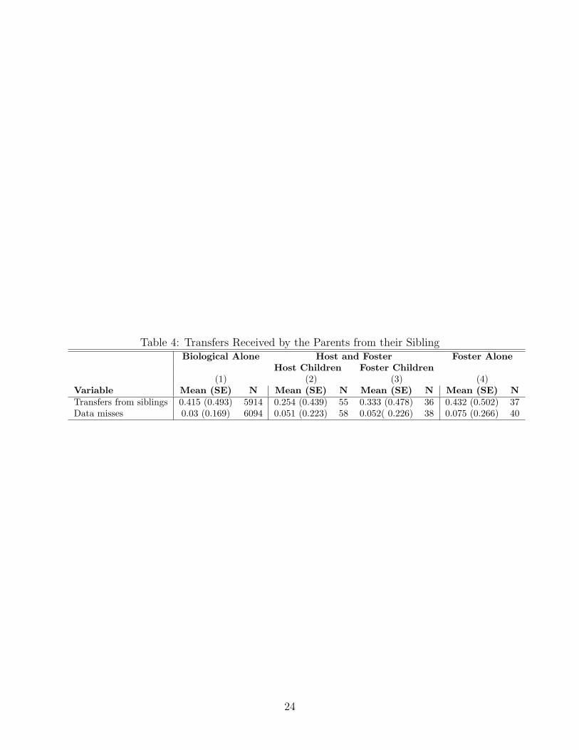
Table 4: Transfers Received by the Parents from their SiblingBiological Alone Host and Foster Foster Alone

Host Children Foster Children(1) (2) (3) (4)

Variable Mean (SE) N Mean (SE) N Mean (SE) N Mean (SE) NTransfers from siblings 0.415 (0.493) 5914 0.254 (0.439) 55 0.333 (0.478) 36 0.432 (0.502) 37Data misses 0.03 (0.169) 6094 0.051 (0.223) 58 0.052( 0.226) 38 0.075 (0.266) 40

24

Table 5: Probit Estimates and Marginal Effects with Transfers Measures

1 specification 2 specificationVariable Prob. ME Prob. MEIs a Host Child 0.574* 0.077** 0.655** 0.084***with Foster-nephew (0.33) (0.03) (0.33) (0.03)

Is a Foster-nephew 0.520 0.069* 0.624 0.077**living Alone (0.41) (0.04) (0.40) (0.03)

Is a Foster-nephew REF REF REF REFwith host Children

Is a Host Child 0.040 0.007 0.187 0.029with Foster-grand-child (0.42) (0.07) (0.41) (0.06)

Is a Foster-grand-child 0.638 0.077** 0.816* 0.087***with Host Children (0.47) (0.04) (0.48) (0.03)

Is a Foster-grand-child 0.619* 0.111* 0.706** 0.127*living Alone (0.36) (0.07) (0.35) (0.07)

Receives Transfers 0.188 0.032 0.197 0.032(0.21) (0.03) (0.22) (0.03)

Transfers miss -0.206 -0.040(0.27) (0.06)

Gender -0.099 -0.017 -0.210 -0.036(0.17) (0.03) (0.17) (0.03)

Age -0.119** -0.021*** -0.144*** -0.025***(0.05) (0.01) (0.05) (0.01)

Both Parents -0.156 -0.026 -0.163 -0.027(0.27) (0.04) (0.25) (0.04)

Educ. Mother 0.200** 0.035** 0.199** 0.034**(0.09) (0.02) (0.09) (0.02)

Educ. Father2 -0.032 -0.006 -0.042 -0.007(0.07) (0.01) (0.07) (0.01)

Mean Age 0.018 0.003 0.017 0.003(0.01) (0.00) (0.01) (0.00)

Consump. pc log 0.264** 0.046* 0.290** 0.050**(0.13) (0.02) (0.13) (0.02)

Rural 0.136 0.024 0.046 0.008(0.22) (0.04) (0.21) (0.04)

Constant -1.795 -1.618(1.62) (1.60)

Pseudo R-squared 0.143 0.143 0.167 0.167Log LR -119.5873 -119.5873 -131.7302 -131.7302N Cluster 220 220 247 247N 360 360 399 399

a* p<0.10, ** p<0.05, *** p<0.01bIn households where the father is absent, we replace the education value by 0 to

not loose observation 25