Biological Modeling of Neural Networks:
26
Biological Modeling of Neural Networks: Week 15 – Fast Transients and Rate models Wulfram Gerstner EPFL, Lausanne, Switzerland 15.1 Review Populations of Neurons - Transients 15.2 Rate models - Week 15 – transients and rate models
-
Upload
shoshana-gallagher -
Category
Documents
-
view
17 -
download
2
description
Week 15 – transients and rate models. 15 .1 Review Populations of Neurons - Transients 15 .2 Rate models -. Biological Modeling of Neural Networks:. Week 15 – Fast Transients and Rate models. Wulfram Gerstner EPFL, Lausanne, Switzerland. - PowerPoint PPT Presentation
Transcript of Biological Modeling of Neural Networks:
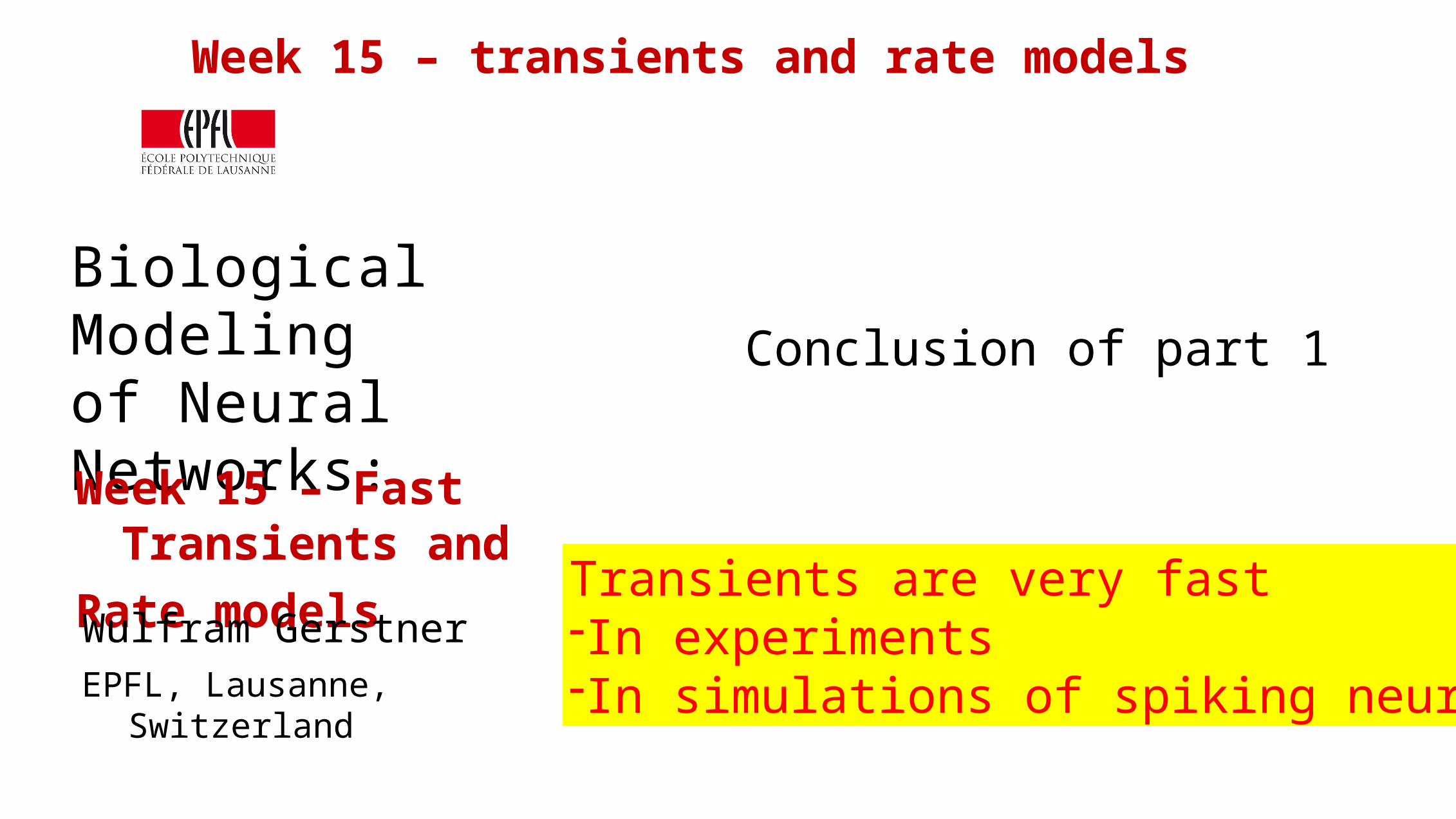
Biological Modeling of Neural Networks:
Week 15 – Fast Transients and
Rate models
Wulfram GerstnerEPFL, Lausanne, Switzerland
15.1 Review Populations of Neurons - Transients15.2 Rate models
-
Week 15 – transients and rate models
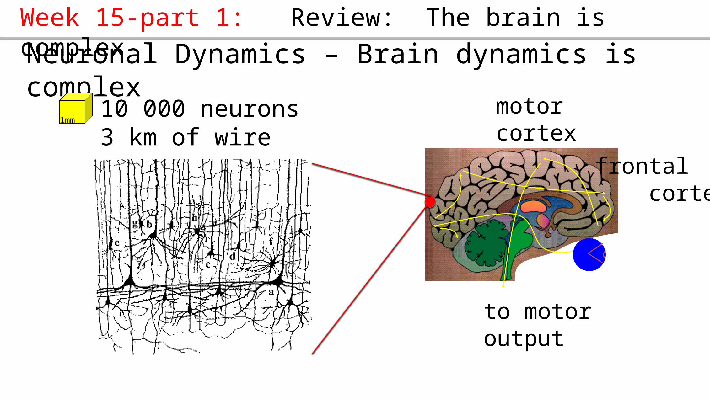
Neuronal Dynamics – Brain dynamics is complex
motor cortex
frontal cortex
to motoroutput
10 000 neurons3 km of wire
1mm
Week 15-part 1: Review: The brain is complex
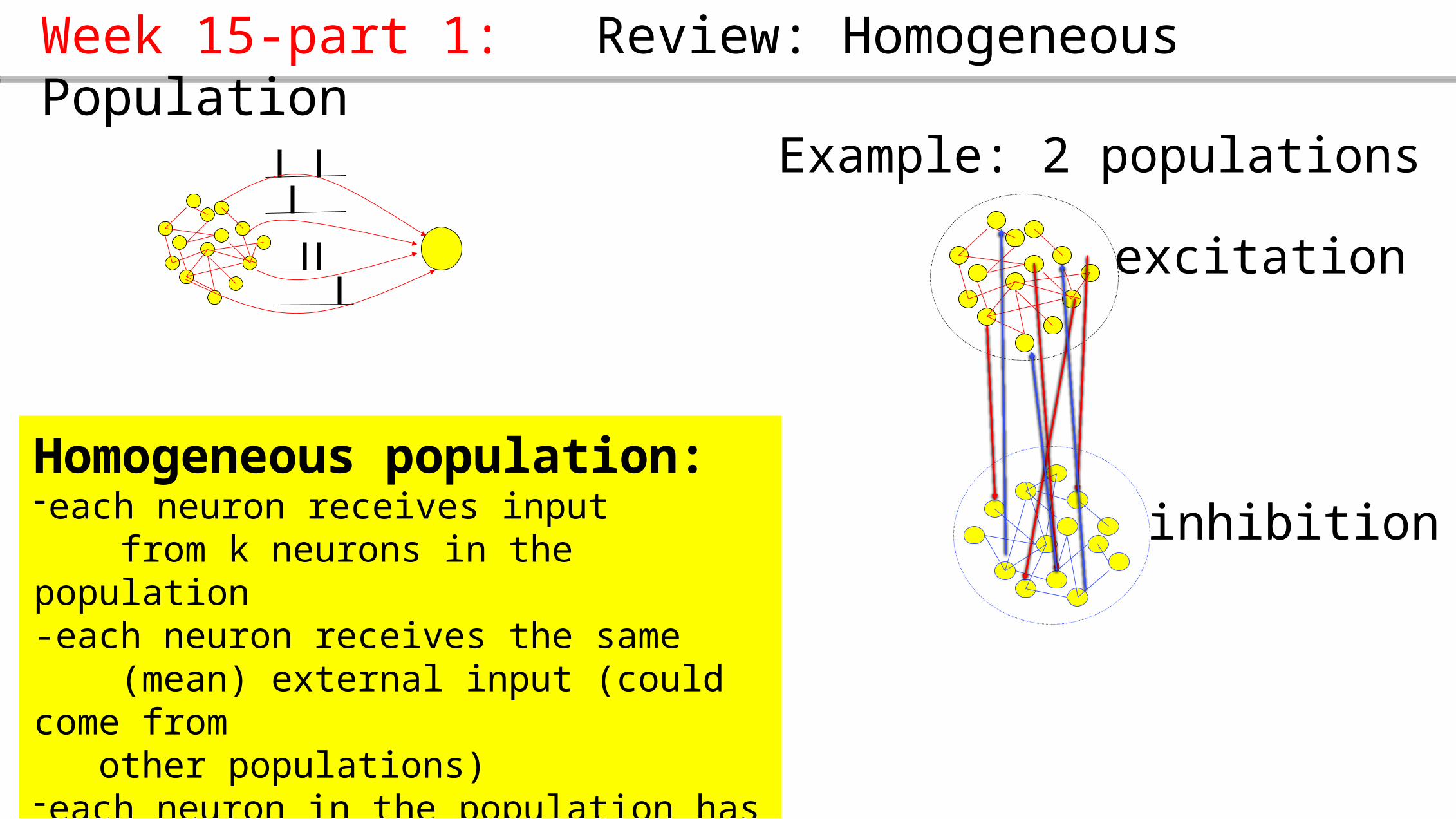
Homogeneous population:-each neuron receives input from k neurons in the population-each neuron receives the same (mean) external input (could come from other populations)-each neuron in the population has roughly the same parameters
Week 15-part 1: Review: Homogeneous Population
excitation
inhibition
Example: 2 populations

I(t)
)(tAn
Week 15-part 1: Review: microscopic vs. macroscopic
microscopic:-spikes are generated by individual neurons-spikes are transmitted from neuron to neuron
macroscopic:-Population activity An(t)-Populations interact via An(t)

I(t)
)(tAn
Week 15-part 1: Review: coupled populations

Populations: - pyramidal neurons in layer 5 of barrel D1 - pyramidal neurons in layer 2/3 of barrel D1 - inhibitory neurons in layer 2/3 of barrel D1
Week 15-part 1: Example: coupled populations in barrel cortex Neuronal Populations
= a homogeneous group of neurons (more or less)
100-2000 neurons per group (Lefort et al., NEURON, 2009)
different barrels and layers, different neuron types different populations

Experimental data: Marsalek et al., 1997
Week 15-part 1: A(t) in experiments:light flash, in vivo
PSTH, single neurons
alignedPSTH, many neurons in V1 (solid)V4 (dashed)

Experimental data: Sakata and Harris, 2009
Week 15-part 2: A(t) in experiments: auditory click stimulus

Experimental data: Tchumatchenko et al. 2011
See also: Poliakov et al. 1997
Week 15-part 1: A(t) in experiments: step current, (in vitro)

Week 15-part 1: A(t) in simulations of integrate-and-fire neuronsSimulation data: Brunel et al. 2011
Image: Gerstner et al.,Neuronal Dynamics, 2014

Week 15-part 1: A(t) in simulations of integrate-and-fire neuronsSimulation data:
Image: Gerstner et al.,Neuronal Dynamics, 2014
Biological Modeling of Neural Networks:
Week 15 – Fast Transients and
Rate models
Wulfram GerstnerEPFL, Lausanne, Switzerland
Week 15 – transients and rate models
Transients are very fast-In experiments-In simulations of spiking neurons
Conclusion of part 1

h(t)
0
( ) ( )h t s I t s ds
Input potential
Week 15-part 2: Rate model with differential equation
( ) ( ( ))A t g h t
I(t)
( ) ( ) ( )dh t h t R I t
dt
Differential equation can be integrated!, exponential kernel

A(t)
h(t)
0
( ) ( ) ...h t s I t s ds
Input potential
Week 15-part 2: Rate model : step current
( ) ( ( )) ( ( ) ( ) )A t g h t g s I t s ds
I(t)
Example LNP rate model: Linear-Nonlinear-Poisson Spikes are generated by a Poisson process, from rate model

A(t)
h(t)
0
( ) ( ) ...h t s I t s ds
Input potential
Week 15-part 2: Wilson-Cowan model : step current
( ) ( ) ( ( ))dA t A t g h t
dt
I(t)
I(t)
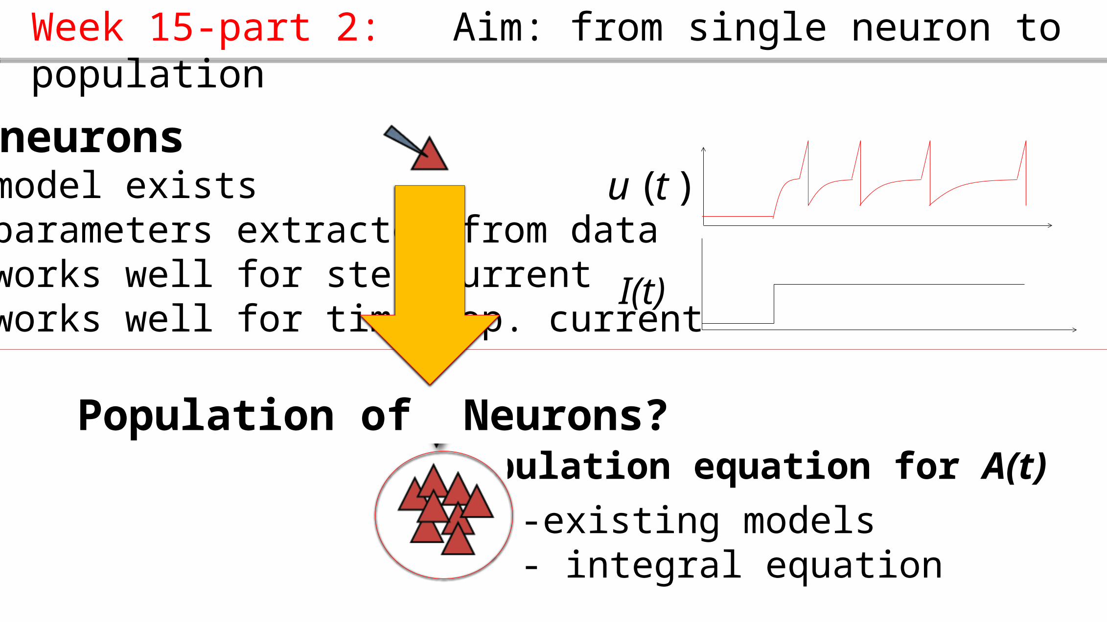
Population of Neurons?
( )u tSingle neurons - model exists - parameters extracted from data - works well for step current - works well for time-dep. current
Population equation for A(t)
Week 15-part 2: Aim: from single neuron to population
-existing models- integral equation
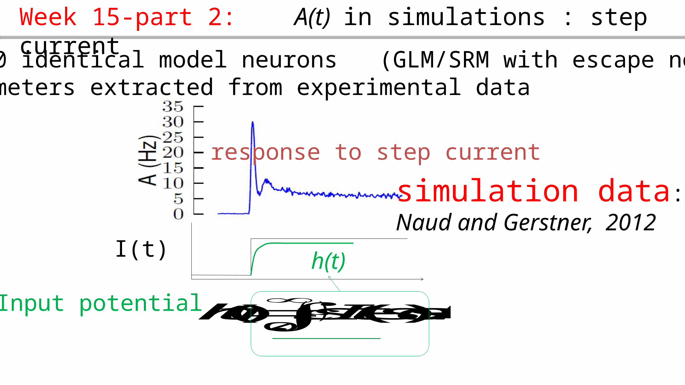
25000 identical model neurons (GLM/SRM with escape noise)parameters extracted from experimental data
response to step current
I(t) h(t)
0
( ) ( ) ...h t s I t s ds
Input potential
simulation data: Naud and Gerstner, 2012
Week 15-part 2: A(t) in simulations : step current

I(t)
Rate adapt.
( )( ) ( ( )) h tA t f h t e
optimal filter(rate adaptation)
Benda-Herz
Week 15-part 2: rate model
LNP theory
simulation
Simple rate model: - too slow during the transient - no adaptation

I(t)
Rate adapt.
( )( ) ( ( )) h tA t f h t e
optimal filter(rate adaptation)
Benda-Herz
Week 15-part : rate model with adaptation
simulation
LNP theory

Rate adapt.
optimal filter(rate adaptation)
Benda-Herz
Week 15-part 2: rate model
Simple rate model: - too slow during the transient - no adaptation
Adaptive rate model: - too slow during the transient - final adaptation phase correct
Rate models can get the slow dynamics and stationary state correct, but are wrong during transient
h(t)
I(t) ?
( ) ( ( )) ( ( ) ( ) )A t f h t f s I t s ds A(t)
A(t) ))(()( tIgtA
potential
A(t) ( ) ( ) ( ( ))dA t A t f h t
dt
t
tN
tttntA
);(
)(populationactivity
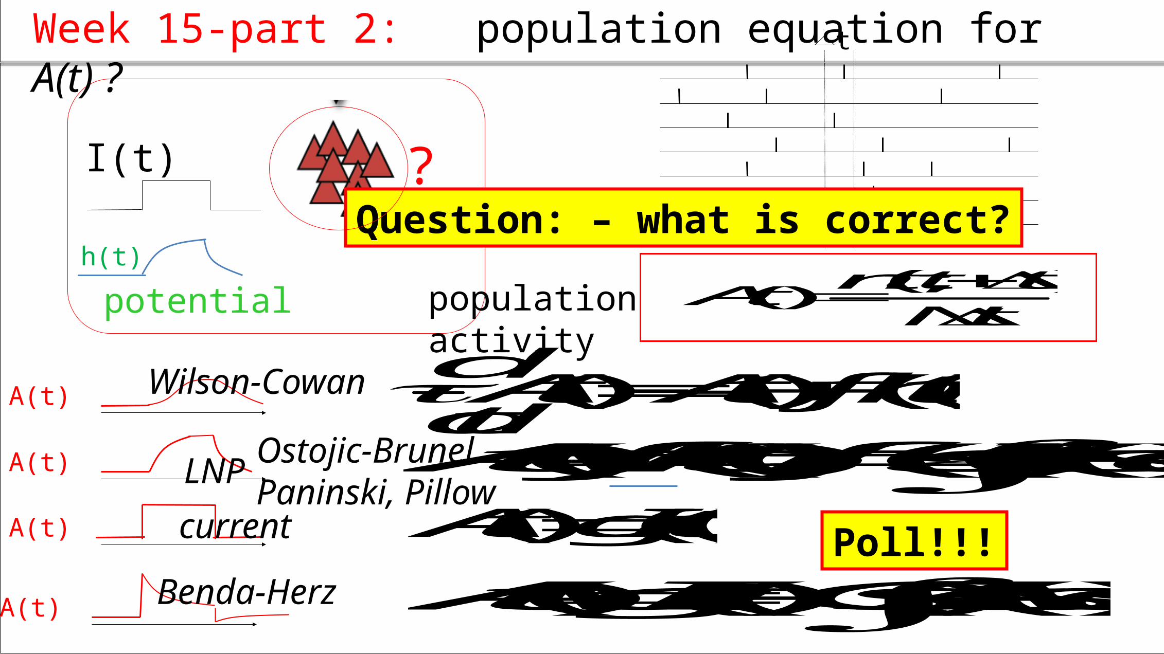
Question: – what is correct?
Poll!!!
A(t) ( ) ( ( ) ( ) ( ) )A t g I t G s A t s ds
Wilson-Cowan
Benda-Herz
LNP
current
Ostojic-BrunelPaninski, Pillow
Week 15-part 2: population equation for A(t) ?
optimal filter(rate adaptation)
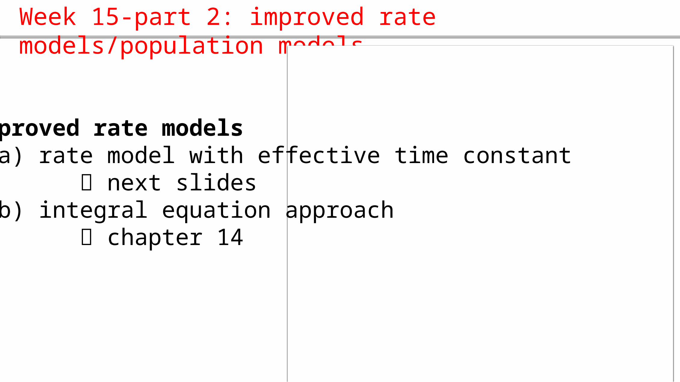
Week 15-part 2: improved rate models/population models
Improved rate models a) rate model with effective time constant next slides b) integral equation approach chapter 14
h(t)
0
( ) ( )h t s I t s ds
Input potential
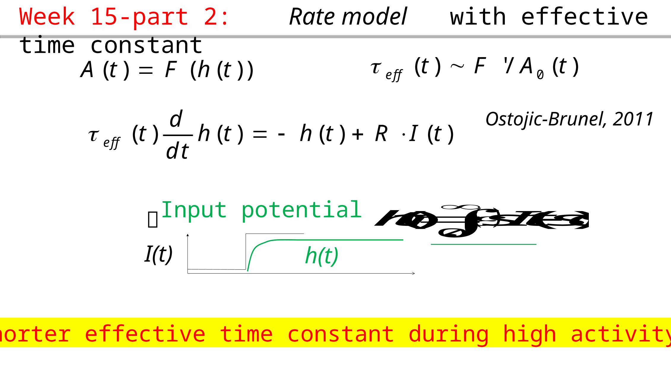
Week 15-part 2: Rate model with effective time constant
( ) ( ( ))A t F h t
I(t)
( ) ( ) ( ) ( )eff
dt h t h t R I tdt
0( ) '/ ( )eff t F A t
Ostojic-Brunel, 2011
Shorter effective time constant during high activity

Week 15-part 2: Rate model with effective time constant
( ) ( ( ))A t F h t
( ) ( ) ( ) ( )eff
dt h t h t R I tdt
0( ) '/ ( )eff t F A t
Ostojic-Brunel, 2011
Shorter effective time constant during high activityTheory fits simulation very well
Image: Gerstner et al.,Neuronal Dynamics, CUP 2014
optimal filter(rate adaptation)
Week 15-part 2; Conclusions
Rate models - are useful, because they are simple - slow dynamics and stationary state correct - simple rate models have wrong transients - improved rate models/population activity models exist

The end
Reading: Chapter 15 ofNEURONAL DYNAMICS, Gerstner et al., Cambridge Univ. Press (2014)