BIOKINEMATIC ANALYSIS OF HUMAN ARM - Ana...
109
i BIOKINEMATIC ANALYSIS OF HUMAN ARM A Thesis Submitted to the Graduate School of Engineering and Sciences of İzmir Institute of Technology in Partial Fulfillment of the Requirements for the Degree of MASTER OF SCIENCE in Mechanical Engineering by Erkin GEZGİN June 2006 İZMİR
Transcript of BIOKINEMATIC ANALYSIS OF HUMAN ARM - Ana...

i
BIOKINEMATIC ANALYSIS OF HUMAN ARM
A Thesis Submitted to the Graduate School of Engineering and Sciences of
İzmir Institute of Technology in Partial Fulfillment of the Requirements for the Degree of
MASTER OF SCIENCE
in Mechanical Engineering
by
Erkin GEZGİN
June 2006 İZMİR

ii
We approve the thesis of Erkin GEZGİN
Date of Signature ………………………… 27 June 2006 Prof. Dr. Tech. Sc. Rasim ALİZADE Supervisor Department of Mechanical Engineering İzmir Institute of Technology ………………………… 27 June 2006 Prof. Dr. Gökmen TAYFUR Department of Civil Engineering İzmir Institute of Technology ………………………… 27 June 2006 Asst. Prof. Dr. Serhan ÖZDEMİR Department of Mechanical Engineering İzmir Institute of Technology ………………………… 27 June 2006 Assoc. Prof. Dr. Barış ÖZERDEM Head of Department İzmir Institute of Technology
………………………… Assoc. Prof. Dr. Semahat ÖZDEMİR
Head of the Graduate School

iii
Anyone who has never made a mistake
has never tried anything new…
Albert Einstein

iv
ACKNOWLEDGMENTS
I would like to express my deepest gratitude to my supervisor Prof. Dr. Tech.
Sc. Rasim ALİZADE for his instructive comments, valued support throughout the all
steps of this study and patience to my questions.

v
ABSTRACT
BIOKINEMATIC ANALYSIS OF HUMAN ARM
Theory of Machines and Mechanisms is one of the main branches of science
including many sub-branches such as biomechanics, human machine systems,
computational kinematics, mechatronics, robotics, design methodology, dynamics of
machinery, gearings and transmissions, cams and linkages, micro machines, nonlinear
oscillations, reliability of machines and mechanisms etc. In this large area of interest,
this study can be matched with the sub groups biomechanics, robotics, computational
kinematics and design methodology. The main concern of the thesis is the
biokinematics of the human arm. In the process of design, a suitable tool for the
kinematics of human arm is investigated as quaternions along with examples. Moreover,
the history of the formulas of Dof is presented as 38 equations with the unique key
controlling parameters that are used in the design of new Cartesian and serial platform
type robot manipulators. Structural syntheses of new manipulators are considered.
Simple serial platform structural groups in subspace λ=3, and general space λ=6 are
presented along with examples. Furthermore, type synthesis of human arm is
accomplished with the new proposed parallel manipulator for the shoulder, elbow and
wrist complex. Finally, computational kinematics of the serial human wrist manipulator
and the geometrical kinematic analysis of the orientation platforms of the new parallel
manipulator design for the human arm are accomplished.

vi
ÖZET
İNSAN KOLUNUN BİOKİNEMATİK ANALİZİ
Ana bilim dallarından biri olan Makina ve Mekanizmalar Teorisi, birçok alanı
kapsamaktadır. Bu alanlardan en önemlileri, biomekanik, insan-makina sistemleri,
sayısal kinematik, mekatronik, robotik, dizayn metodolojisi, makina dinamiği, dişliler
ve aktarma organları, kamlar ve linkler, mikro mekanizmalar, lineer olmayan titreşimler
ve mekanizma güvenilirliği olarak özetlenebilir. Bu kadar geniş bir alan içerisinde, ilgili
çalışma biomekanik, robotik, sayısal kinematik ve dizayn metodolojisiyle
ilişiklendirilebilinir. Tezin ana konusu, insan kolunun biokinematik analizidir. Dizayn
süreci içerisinde, insan kolunun kinematik analizinde kullanılacak önemli bir araç olan
quaternionlar, örneklerle incelenmiştir. Yapısal sentez formullerinin tarihi araştırılmış,
38 farklı denklemde açıklamalarıyla birlikte gösterilmiştir. Bu formuller yeni Kartezyen
ve seri platform tipli robot manipulatörlerin dizaynında kullanılmıştır. Yeni tasarlanan
robot manipulatörlerin yapısal sentezi yapılmış, seri platform robot manipulatörlerinin
alt uzay λ=3 te ve uzay λ=6 daki yapısal grupları gösterilmiştir. İnsan kolunun kategori
sentezi tamamlanmış, omuz, dirsek ve bilek kompleksi için yeni bir parallel robot
manipulatör önerilmiştir. Son olarak seri insan bilek manipulatörünün sayısal
kinematiği ile birlikte, yeni paralel manipulatörün oryantasyon platformlarının
geometrik kinematik analizi yapılmıştır.

vii
TABLE OF CONTENTS
LIST OF FIGURES ........................................................................................................ ix
LIST OF TABLES.......................................................................................................... xi
CHAPTER 1. INTRODUCTION.....................................................................................1
CHAPTER 2. HISTORY OF DEVELOPMENT .............................................................4
2.1. Background.............................................................................................4
2.2. Research Statement...............................................................................14
CHAPTER 3. QUATERNION ALGEBRA ...................................................................16
3.1. Preliminaries .........................................................................................16
3.2. Quaternion Addition and Equality........................................................17
3.3. Quaternion Multiplication.....................................................................20
3.4. Conjugate of the Quaternion.................................................................21
3.5. Norm of the Quaternion........................................................................21
3.6. Inverse of the Quaternion .....................................................................22
CHAPTER 4. STRUCTURAL SYNTHESIS OF SERIAL PLATFORM
MANIPULATORS ..................................................................................24
4.1. Structural Formula ................................................................................24
4.2. Structural Synthesis and Classification of Simple Serial Platform
Structural Groups..................................................................................33
4.3. Structural Synthesis of Parallel Cartesian Platform Robot
Manipulators .........................................................................................37
CHAPTER 5. TYPE SYNTHESIS OF HUMAN ARM ................................................40
5.1. The Clavicle ..........................................................................................41
5.2. The Humerus.........................................................................................44
5.3. The Radius and the Ulna.......................................................................47
5.4. Combined Manipulator for Human Arm ..............................................49

viii
CHAPTER 6. KINEMATICS OF HUMAN WRIST MANIPULATOR.......................51
6.1. Quaternions as a Product of Two Lines................................................51
6.2. Rigid Body Rotations by Using Sequential Method by Quaternion
Operators...............................................................................................55
6.3. Rigid Body Rotations by Using New Modular Method by Quaternion
Operators...............................................................................................56
6.4. Spherical Wrist Motion through Quaternions.......................................59
6.5. Workspaces of the Spherical Wrists .....................................................64
CHAPTER 7. GEOMETRICAL ANALYSIS OF THE HUMAN CLAVICLE AND
ELBOW MANIPULATOR ....................................................................66
7.1. Geometrical Analysis of Spatial 3-Dof Orientation Mechanism
in λ=6 ....................................................................................................66
7.2. Geometrical Analysis of Spatial 2-Dof Orientation Mechanism
in λ=6 ....................................................................................................73
CHAPTER 8. CONCLUSION .......................................................................................77
REFERENCES ...............................................................................................................78
APPENDICES
APPENDIX A. Result of the equations 1
21
11123 )( −−= qqrqqr and
2 1 12 2 1 2 1 2( )r q q r q q
• • •− •−= ............................................................................86
APPENDIX B. Q-BASIC CODE FOR THE CREATION OF THE STRUCTURAL
GROUPS OF SERIAL PLATFORM MANIPULATORS...................88
APPENDIX C. MOTION ANALYSIS OF NEW CARTESIAN ROBOT
MANIPULATORS ...............................................................................90

ix
LIST OF FIGURES
Figure Page
Figure 1.1. Human Shoulder, Elbow, and Wrist Complex ...............................................1
Figure 1.2. Rotation by a Quaternion Operator ................................................................2
Figure 1.3. One of the Structural Groups of Serial Platform Manipulators in 3λ = .......3
Figure 2.1. Primitive Human-like Robots......................................................................14
Figure 4.1. 6 Dof Spatial Serial Platform Robot Manipulator........................................37
Figure 5.1. Structure of Human Arm..............................................................................40
Figure 5.2. Clavicle.........................................................................................................41
Figure 5.3. Clavicle Rotations ........................................................................................42
Figure 5.4. Clavicle Rotations in Detail .........................................................................42
Figure 5.5. 3 Dof Orientation Platform...........................................................................43
Figure 5.6. Humerus and the Shoulder Joint ..................................................................44
Figure 5.7. Scapula Rotations .........................................................................................45
Figure 5.8. Scapula Rotations in Detail ..........................................................................45
Figure 5.9. Humerus Rotations Relative to Scapula, Y-X-Y Sequence .........................46
Figure 5.10. Agile Eye, Optimized3-Dof Spherical Parallel Platform ...........................46
Figure 5.10. Radius and Ulna .........................................................................................47
Figure 5.11. Radius and Ulna Rotations .........................................................................48
Figure 5.12. 2 Dof Orientation Platform.........................................................................48
Figure 5.13. New Manipulator with Variable General Constraints that Mimics
Human Shoulder, Elbow and Wrist Complex ..............................................49
Figure 6.1. Multiplication of Two Lines.........................................................................51
Figure 6.2. Sequential Rotations of 1r ............................................................................55
Figure 6.3. Modular Method Rotations ..........................................................................57
Figure 6.4. Position Vectors of a Spherical Serial Wrist with 2-Dof .............................59
Figure 6.5. Position Vectors of a Spherical Serial Wrist with 3-Dof .............................61
Figure 6.6. Position Vectors of a Spherical Serial Wrist with 4-Dof .............................63
Figure 6.7. Workspace of a Spherical Serial Wrist with 2-Dof......................................64
Figure 6.8. Workspace of a Spherical Serial Wrist with 3-Dof......................................65
Figure 6.9. Workspace of a Spherical Serial Wrist with 4-Dof......................................65

x
Figure 7.1. Orientation Platform (Red) of the New Manipulator Design.......................66
Figure 7.2. Orientation Platform (Closed View) ............................................................66
Figure 7.3. Sphere with Radius “r” whose Center is Fixed at the Origin .......................67
Figure 7.4. Sphere with Radius “r” whose Center is Away from the Origin..................67
Figure 7.5. Generalized Orientation Mechanism............................................................69
Figure 7.6. Construction Parameters of Upper Platform (a, b, c) ...................................70
Figure 7.7. 2 Dof Orientation Platform (Red) of the New Manipulator Design.............74
Figure 7.8. 2 Dof Orientation Platform (Closed View) ..................................................74
Figure 7.9. 2-Dof Orientation Platform (Base)...............................................................74
Figure 7.10. Generalized 2-Dof Orientation Platform....................................................75
Figure C.1. Raw Motion Analysis ..................................................................................90
Figure C.2. Raw Motion Analysis ..................................................................................91
Figure C.3. Raw Motion Analysis ..................................................................................92
Figure C.4. Raw Motion Analysis ..................................................................................93
Figure C.5. Raw Motion Analysis ..................................................................................94
Figure C.6. Raw Motion Analysis ..................................................................................95
Figure C.7. Raw Motion Analysis ..................................................................................96
Figure C.8. Raw Motion Analysis ..................................................................................97
Figure C.9. Raw Motion Analysis ..................................................................................98

xi
LIST OF TABLES
Table Page
Table 2.1. Formulas for Structural Analysis and Synthesis..............................................8
Table 4.1. New Parallel Cartesian Manipulator Types ..................................................29
Table 4.2. Simple Structural Groups of Serial Platform Manipulators in λ=6 ...............35
Table 4.3. Simple Structural Groups of Serial Platform Manipulators in λ=3 ...............36
Table 4.4. Variation of Actuators for Simple Structural Group RRR (λ=3) of Parallel
Cartesian Platform Robot Manipulators ......................................................39

1
CHAPTER 1
INTRODUCTION
Kinematic analysis of robot manipulators can be carried out by using many
tools, such as screw theory, quaternions, biquaternions, rotation and transformation
matrices etc. Each has its own advantages and disadvantages when compared in
different tasks; for instance, pure rotation motions can be easily and precisely analysed
by quaternion operators, while rotation matrices yield computational errors and lack
computational efficiency. On the other hand, quaternions can not be used solely in the
analysis of translation motions, where transformation matrices are capable. As a result
of the fact, it is very important to select the right tool for the desired application for the
ease of use. From this point of view, the first step of the scientific investigation was
assigned to find the best promising tool for the analysis of human arm motion.
Figure 1.1. Human Shoulder, Elbow, and Wrist Complex (Source: CMBBE’99)
After a detailed research on human shoulder, elbow, and wrist complex,
(Fig. 1.1), it was appeared that nearly all of the joints of the complex have limited
spherical motions; therefore, analysis of rotations has taken a great priority. So that, due

2
to their precision, computational speed and efficiency in rotations, quaternions were
selected as the tool for motion analysis of the human arm, (Fig. 1.2).
Figure 1.2. Rotation by a Quaternion Operator (Source: ARTEMMIS)
The investigation was continued by the study of quaternion algebra and
operators for rotations. However, it was seen that, regular sequential rotation method of
quaternions can not simulate the exact human motion. Thus, for one step ahead to reach
the natural motion of human, a new rotation sequence by quaternions was developed
and named modular method. The new method was applied to the serial 2-DoF, 3-DoF
and 4-DoF spherical wrist and compared by the traditional sequential method to prove
the results. Including a new representation of quaternion rotation operator, the modular
method was proposed in IFToMM International Workshop of Computational
Kinematics, CK2005 Italy.
Later in time, another important concept in the design of robot manipulators was
started to be investigated; that is, structural synthesis. Being one of the most important
steps in design, structural synthesis provides the calculation of the desired degrees of
freedom of the robot manipulators. Over 250 years, starting by Euler, many
formulations have been created to fulfil the calculations for different types of robots;
also, in each period new parameters have been introduced.
After collecting all of the information from a deep history about structural
synthesis, the first time in literature, a compact table including all of the structural

3
formulas of the related years and authors were introduced with the definitions of
parameters that are used in the formulations. Using the collected information and table
as a guideline, a new structural formula for Cartesian robot manipulators was proposed
and nine new Cartesian robot manipulators were constructed with respect to the new
formulation. Parallel to this study, structural synthesis of serial platform type
manipulators with lower and higher kinematic pairs according to their structures was
also examined. Serial platform manipulators were created according to the development
of the platforms and closed loops by the new interpretation of the Alizade formula. Also
structural groups of serial platform manipulators in subspace 3λ = and space
6λ = were tabulated in two separate tables, (Fig. 1.3). The complete work about
structural synthesis was accepted by IFToMM Journal of Mechanism and Machine
Theory (MMT40-129).
Figure 1.3. One of the Structural Groups of Serial Platform Manipulators in 3λ =
The last part of the investigation was the design of a new manipulator with
variable general constraints that mimics human shoulder, elbow and wrist complex. The
manipulator was designed with two orientation platforms in space 6λ = and one
spherical platform in subspace 3λ = . After its structural synthesis was completed, and
the animations were carried out, geometrical kinematic analysis of its orientation
platforms was accomplished.

4
CHAPTER 2
HISTORY OF DEVELOPMENT
2.1. Background
Hypercomplex numbers, quaternions, give a wide field of applications in the
area of computational kinematics. First applications, which quaternions have been
found more than 150 years ago, were the description of motion of the rigid body
(Hamilton 1866, WEB_1 2005). Hypercomplex numbers allow simplifying the practical
calculations in a drastic way. At the same time they are applied to such problems of
modern computational kinematics (Porteous 1921, Martinez et al. 2000). From
geometric point of view, a quaternion is the quotient of two directed lines in space, or
operator, which changes one directed line into another. Sir W.R. Hamilton (Britannica
1886) describes that, if motion in one direction along a line is treated as positive, motion
in the opposite direction along the same line is negative.
In the computational kinematics of a rigid system, we have to consider one set of
rotations with regard to the axes that are fixed in the system. Using usual methods, we
have a problem of complexity. Each quaternion formula is a preposition in spherical
trigonometry and the singular quaternion operator q ( ) q-1 turns any directed line,
conically, through a definite angle about a definite axis (Hamilton 1866).
The topological geometry in spatial kinematics is discussed in (Porteous 1921),
and the representation of spherical displacements and motions are described by the
rotation group of unit quaternions.
Angeles (1988) introduced the theory of vector and scalar invariants of a rotation
tensor as a function of time of a spherical motion. Nixravesh et al. (1985) introduced the
method which is based on a sequence of matrix computation, and identities for relating
a representation of spherical motion with their corresponding velocity and acceleration
vectors. Larochelle (2000) used planar quaternions to create synthesis equations for
planar robots, and created a virtual reality environment that could promote the design of
spherical manipulators. Martinez et al. (2000) presented quaternion operators for
describing the position, angular velocity and angular acceleration for a spherical motion

5
of a rigid body with respect to the reference frame. Liu et al. (2003) described the
physical model of the solution space for the spherical 3-DoF serial wrists, the
classification of the reachable and dexterous workspace, and the atlases of the work
spaces.
When an end effector of the spherical 3-DoF serial wrist reaches the tools, it will
work as a spherical four-bar mechanism with 1-DoF. Several discussion of the design of
spherical four-bar mechanisms widely studied in the literature and in the last one was
the study of Alizade et al. (2005) that applied superposition method for linearization of
nonlinear synthesis equations in the problem of analytical synthesis described by five
precision points.
Structural synthesis problem is the first step in the design of new robot
manipulators and the fundamental concept in robot design. The mobility of robotic
mechanical system describes the number of actuators needed to define the location of
end-effectors. It is important that the mobility or the degrees of freedom of robot
manipulators (M>1) indicates the number of independent input parameters to solve the
problem of all the configuration of robots or a kinematic chain with several actuators. If
mobility of the kinematic chain is equal to zero (M=0) and can not be split into several
structural groups, we will get a simple structural group. Combining the simple structural
groups with actuators, we can get serial or parallel robot manipulators. IFToMM
terminology defines “manipulator that controls the motion of its end-effector by means
of at least two kinematic chains going from the end-effector towards the frame” as
parallel manipulator. In parallel manipulators, two platforms can not be connected by
kinematic pairs to each others.
Serial platform manipulators control the motion of the platforms by means of at
least two platforms, which are connected by kinematic pairs, and other kinematic chains
going from the platforms towards the frame. Several connections of the links in series
for gripping and the controlled movement of objects are called serial manipulators.
Combination of serial and parallel manipulators gives hybrid robot manipulators.
Complex robot manipulators consist of independent loops with variable general
constraint (λ=2, 3, 4, 5, 6).
The history of works about the number of independent loops was done by L.
Euler (Courant 1996). Then in the second half of the XIX century, the first structural
formulas of mechanisms were created (Chebyshev 1869, Sylvester 1874, Grübler 1883,
Somov 1987, Gokhman 1889). As shown in Table 2.1, in the mobility equations we can

6
find concepts of the number of independent loops (L), degrees of freedom or mobility of
mechanisms (M), the loop motion parameters (λ), the number of joints (j), number of
moving links (n), number of mobility of kinematic pairs (f), independent joint
constraints (s), number of passive mobilities (jp), and the number of overclosing
constraints (q). To describe and compare the structural formulas and the parameters in
structural analysis and synthesis of robotic mechanical system, the unique key
controlling parameters are used as shown in Table 2.1.
Furthermore, the concepts of the structural formulas and simple structural groups
were developed in the first half of the XX century (Koeings 1905, Assur 1952, Muller
1920, Malushev 1923, Kutzbach 1929, Kolchin 1932, Artobolevskii 1939, Dobrovolskii
1939). As shown in Table2.1, some new concepts in the problem of structural analysis
and synthesis of mechanisms had been reached as number of screw pairs (Sc), simple
structural groups with zero mobility (M=0), number of kinematic pairs with i class (pi,
where i is the number of joint constraint), number of links with variable length (nv),
variable general constraint (λK), and the family of the elementary closed loop (dK =6-
λK).
During the second half of the XX century, the productive results to find general
methods for determination of the mobility of any mechanisms had been obtained
(Moroshkin 1958, Voinea et al. 1959, Paul 1960, Rössner 1961, Boden 1962, Ozol
1962, Waldron 1966, Manolescu 1968, Bagci 1971, Antonescu 1973, Freudenstein et
al.1975, Hunt 1978, Herve 1978, Gronowicz 1981, Davies 1981, Agrawal et al. 1987,
Dudita et al. 1987, Angeles et al. 1988, Alizade 1988, McCarthy 2000). In the
calculation of mechanism mobility, the following new parameters were used (Table 2.1)
: rank of linear independent loop equations or the order of the equivalent screw system
of the closed loop (r), relative displacements of the joint (m), number of independent,
scalar, differential loop-closure equations (λK), the rank of the coefficient matrix (r(j)),
finite dimensional vector space (d(v)), new formula of the number of independent loops
(L=jB-B-cb, where jB is the total number of joints on the platforms, and cB is the total
number of branches between moving platforms and B is the number of moving
platforms), serial open chains connecting to ground or total number of robot legs (cl),
and the degree of constraint of the platform (U). It should be noted that, branches are
the kinematic chains that connects mobile platforms to each other, and legs are the
kinematic chains that connects mobile platforms to the fixed frame.

7
In the beginning of XXI century, further developments of robotic science has
arisen the interest in scientific investigations. New parameters in the structural formulas
describing the real physical essences should be created in the new investigations and be
more suitable for the use in practice in new subjects. In this direction, there are several
studies (Huang 2003, Alizade et al. 2004, Gogu 2005, Alizade et al. 2006). In the
calculation of degrees of freedom of mechanisms, the new parameters are used in the
structural formulas, as a new formulation of the number of independent loops (L=c-B)
and new formulation for simple structural groups (Êfi=λ(c-B)), where c=cb+cl+ch, ch
is the number of hinges between moving platform, and c is the total number of
connections. Also note that, hinges are the revolute pairs that connect mobile platforms
to each other. For describing and comparing structural formulas and parameters in
structural analysis and synthesis of robotic mechanical system the unique key
controlling parameters are used as shown in Table 2.1.
The basis of structural synthesis of manipulators are based on the principles of
truss kinematical unchanging. Determination of indivisible groups as simple structural
groups and creating different new manipulators by using their combination had been
done by striving to systematize investigation methods of manipulators.
Firstly Assur (1982) developed the concept of the open chain and utilized this
concept for plane structure classification. Secondly, the problem of structural synthesis
and analysis was investigated by Malushev (1929). The problem of structural synthesis
for spatial mechanisms was introduced by Artobolevskii (1939). The task of structural
synthesis was solved by using method of developing closed loops. The classes of
structural groups are defined by the number of links of the closed loops and the order is
equal to the number of legs.
According to the method of structural synthesis that is given by Baranov (1952),
spatial and plane structural groups have been created from corresponding trusses, and
class of simple structural groups are defined by the number of closed loops. Kolchin
(1960) has introduced concept of passive constraints to account for existence of the
paradoxical mechanisms. That concept has not presented any means for identifying the
geometric conditions that determine the general constraints.

8
Table 2.1. Formulas for Structural Analysis and Synthesis
Equations Authors Commentary
1 1L j l= − +
l is the number of links; j is the number of joints
L. Euler, 1752
L is the number of independent loops;
2
3 2 1 0
10 1
23 1
m
m
m m
l j
j j l
j l l n l
− − =
< − < +
> − = = −
P. L. Chebyshev,
1869
Eq. for planar mech. with 1 DoF
mj is the number of moving
joints
ml = n is the number of
moving links
3 3 2 4 0
1
l j
j n
− − =
= −
J. J. Sylvester, 1874
Eq. for planar mech. with 1 DoF
4
1
) 3 2 3
) 3 2 4 0
) 2 3 0
) 3 2 4 0
) 5 6 7 0
6( 1) 5
a M l j
b l j q
c l j
d l j q C
e H l
or M l p
= − −
− − + =
− − =
− − + − =
− + =
= − −
q is the number of overclosing constraints
1p is the one mobility joints
C is the number of cam pairs H is the number of helical joints
M. Grübler, 1883, 1885
M is mobility of mechanisms. DoF depends from the rank of functional
determinant (r=3, 2) a) DoF for planar mech.
b) Eq. for kinematic chains with revolute R and prismatic P pairs
c) Eq. for plane mech. just with prismatic P pairs
d) Eq. for kinematic chains with revolute, prismatic and
cam pairs e) DoF of spatial mech. with
helical joints
5
) ( 1)( 1) 2
) ( 1)( 1) 2
) ( 1) 5
5 7, 6, 1,
1
u
i
u p
a l
b l q K
c M l f j L q
l L
K j
λ ν
λ ν
ν λ ν
− − + =
+ + − − + =
= − + − − +
= + = = −
= −
∑∑
∑
pj is the passive mobilities in the joints
if is the mobility of kinematic pairs
P.O. Somov, 1887
a) Eq. for plane (λ=3) and spatial (λ=6) mech. (M=1) b) Eq. for plane and spatial
mech. (M=1) c) Somov’s universal structural formula
λ is the number of independent parameters describing the position of
rigid body (general constraint parameter)
6
) ( 1) 1a l Sλ − − =
( ) iS i fλ= −∑ is the total number of
independent joint constraints
) 1
) ( ) 1
ib f L
c j L S
λ
λ
− =
− − =
∑
Kh. I. Gokhman, 1889
a) Eq. for plane and spatial mech. (M=1)
b) Loop mobility criterion (M=1)
c) Eq for mech. (M=1) Eqs. (a) and (c) gives Euler’s
equation
7 6M n S= − G. Koeings,
1905
Mobility Eq. for spatial mech.
(similar to Gokhman Eq.)
8 3 2 0n j− = L. V. Assur,
1916 Eq. for simple structural
groups
9
( 1) ( 1) 0
( 1)s
s
S l
M n S
λ λ λ
λ λ
− − + + =
= − −
sS is the number of screw pairs
R. Muller, 1920
Eq. for kinematic chains with screw pairs
(Similar to M. Grubler Eq.)

9
Table 2.1 (cont.). Formulas for Structural Analysis and Synthesis
Equations Authors Commentary
10
5
1
6( 1) i v
i
M l ip q n=
= − − + −∑
ip is the kinematic pairs with i class
i = number of joint constraint
A. P. Malushev, 1923
Universal Somov-Malushev’s mobility Eq.
vn is the number of links
with variable length
11 1
1
( 1)
( 1) ( )
j
i
i
j
i
i
M l j f
M l i f
λ
λ λ
=
=
= − − +
= − + −
∑
∑
K. Kutzbach, 1929
Other form of universal mobility Eq.
12 23( 1) 2( )M l P R K p= − − + + −
P is the number of prismatic pairs R is the number of revolute pairs
N. I. Kolchin, 1932-1934
Structural formula for planar mechanisms.
K is the number of higher pairs with pure roll or pure slippage
2p is the number of higher
pair with rolling and slipping
13 1 1
6j L
j K
i K
M n S d q= =
= − + +∑ ∑
6K Kd λ= − is the family of the elementary
closed loop or the number of independent constraints in the loops
I. I. Artobolevskii, 1935
Other form of universal mobility Eq. First time in mobility Eq., it is used
variable general constraint as variable number of
independent close loops family.
Kλ is the variable general
constraint
14
1
1
( )
2,....,6
i
i
M n i p qλ
λ λ
λ
−
=
= − − +
=
∑
V. V. Dobrovolskii, 1939
Other form of universal structural formula
15
)
)
1,...,5 2,...,6
)
i
i
i
i
a M ip r
b M ip L
i
c L j n
λλ
λ
λ
= −
= −
= =
= −
∑
∑ ∑
U. F. Moroshkin, 1958
a) Structural Eq. of system with the integrable joining b) Eq. of the DoF with
variable general constraint c) Number of independent
close loops
r λ= is the rank of linear independent loop
16 1 1
j L
i K p
i K
M f r j= =
= − −∑ ∑
1
j
i
i
f=∑ is the total number DoF of joints with
revolute, prismatic and helical joints;
R. Voinea and M. Atanasiu,
1959
Mobility Eq of a complex mechanisms
1≤rK≤6 is the rank of screw system
17 1L j l= − + B. Paul, 1960
Using formula #1, it was created topological condition of criterion for the degree of constraint of plane kinematic
chains
18 1
6( 1)j
i
i
M f j l=
= − − +∑ W. Rössner ,
1961
The mobility Eq. taking into consideration Euler’s
formula # 1

10
Table 2.1 (cont.). Formulas for Structural Analysis and Synthesis
Equations Authors Commentary
19 1
6( 1) 3( 1)j
i
i
M f j l j l=
= − − + − − +∑ H. Boden,
1962
Mobility Eq., consisting from the planar and the spatial
loops
20
1
1
) 6
) 3
) 2( 1)
) 2
j
i
i
j
i
i
a M f L q
b M f L q
c M l j q
d M j L q
=
=
= − +
= − +
= − − +
= − +
∑
∑ O. G. Ozol,
1962
a), b), and c) mobility Eq.s for variable general
constraint, as λ=6, 3, 2 with excessive constraints d) mobility Eq. for
cylindirical mechanisms (λ=2)
21 M F r= − F is the relative freedom between links
K. J. Waldron, 1966
Mobility Eq of closed loop r is the order of the
equivalent screw system of the closed loop
22 5
1
(6 ) (6 )i
i r
M i p d L= +
= − − −∑ N. Manolescu,
1968
Mobility Eq. with the parameter of the family of the elementary closed loop.
23
5
1 1
6( 1) (6 )L
i K
i K
p
M l i f d
q j
= =
= − − − + +
+ −
∑ ∑
∑ ∑
C. Bagci, 1971
Mobility Eq. to calculate DoF of motion in a
mechanism similar to Eq. #
13 by adding parameter pj
24 5
1
(6 )( 1) ( )a a i
i
M d l i d p=
= − − − −∑ P. Antonescu,
1973
Mobility formulas with different values for the motion coefficient λ
(formula #14)
25
1 1
1 1
1
1
)
)
)
)
2 , 3, 4 , 5, 6
E L
i K
i K
j L
i K
i K
E
i
i
j
i
i
a M m
b M f
c M m L
d M f L
λ
λ
λ
λ
λ
= =
= =
=
=
= −
= −
= −
= −
=
∑ ∑
∑ ∑
∑
∑
E is the total number of independent displacement variable
im is the relative displacements of the joints
if is the relative joint motion when im
correspond in 1:1 with DoF in joints
F. Freudenstein, R. I. Alizade,
1975
Mobility Eq.s without exception
a) and b) mobility Eq.s are used for mechanisms which contain mixed independent loops with variable general
constraint. c) and d) Mobility equations of mechanisms with the same
number of independent, scalar loop closure equations in each independent loop.
Kλ is the number of
independent, scalar, differential loop closure
equations
λ is the DoF of space where the mechanism operates
26 1
( 1)j
i
i
M l j fλ=
= − − +∑ K. H. Hunt,
1978 Mobility Eq. coming from
Eq. 25d using Eq 1
27 1
( 1) ( )j
i
i
M l fλ λ=
= − − −∑ J. M. Herve,
1978
Mobility formula based on the algebraic group structure
of the displacement set

11
Table 2.1 (cont.). Formulas for Structural Analysis and Synthesis
Equations Authors Commentary
28
1
1 1
L L
K Kj
K j K
M Fλ−
= = +
= −∑ ∑ ∑
KjF is the mobility of the joints that is common
between any two loops K and j, and the mobility of the joints in the L loops can be counted once or twice
A. Gronowicz, 1981
Mobility Eq. for multi loop kinematic chains
29
1
j
i
i
M f r=
= −∑ T. H. Davies,
1981
Mobility equations similar to Eq. # 15a
r is the rank of the coefficient matrix of constraint
equations
30
1
2
12
1 1 1 1
2
1
1( 2)
2
1( 3 2)
2
NL L L
K Kj i i ni
K K j K i
N
i i ni
i
M F n n F
n n F
λ−
= = = + =
=
= − + + − +
+ − +
∑ ∑∑ ∑
∑
%% %
V. P. Agrawal, J. S. Rao,
1987
Mobility Eq. to any general mechanism with constant or variable general constraints with simple or multiple joints
1N ,
2N is the total number of
internal and external multiple joints respectively
in% , niF%; in , niF is the
number of links and the mobility of simple joints
forming the i th internal and external multiple joints
respectively.
31
1 1
1
)
) ( 1)
j L
e e
i K
i K
L
e
K comj comj
K j
a M f
b M L f
λ
λ
= =
=
= −
= − −
∑ ∑
∑ ∑
comjL is the number of loops with common joint
j e
comjf is the active degree of mobility of the j th
common joint
F. Dudita, D. Diaconescu,
1987
Eq. of a elementary or a complex (multi loop)
mechanisms e
if is the active mobilities in
i th joint e
Kλ is the dimension of the
active motion space
32
( )
( ) ( ) ( )
M nullity J
nullity J d v r J
=
= −
J is the Jacobian matrix; r(J) is the rank of the Jacobin matrix; d(v) is the finite dimensional vector space v
J. Angeles, C. Gosselin,
1988
The mobility Eq. by using the Jacobian matrix of a
simple or multi loop closed kinematic chain without
exception
33
1
1
1
)
) ( )
) ( )
) ( )
B b
E
i B b
i
j
i B b
i
j
i B b
i
p
p
a L j B c
b M m j B c q j
c M f j B c q j
d f j B c
λ
λ
λ
=
=
=
= − −
= − − − + −
= − − − + −
= − −
∑
∑
∑
B is the number of mobile platform;Bj is the
total number of joints on the mobile platforms
R. I. Alizade, 1988
a) A new formula of number of independent loops b) and c) are structural formulas as a function of number of branches, platforms and sum of
mobility of kinematic pairs and other parameters
d) Eq. for simple structural groups (λ=6,5,4,3,2)
bc is the total number of
branches between mobile platforms

12
Table 2.1 (cont.). Formulas for Structural Analysis and Synthesis
Equations Authors Commentary
34 1
( )lc
i
i
M fλ λ=
= − −∑
( )ifλ − is the degree of constraint of the
platform
J. M. McCarthy, 2000
Mobility Eq. of a parallel manipulator
35 1
(6 )( 1)j
i
i
M d l j f q=
= − − − + +∑ Z. Huang, Q .C. Li, 2003
Structural formula for parallel mechanisms
36
, ,
1
1
2
) ( )
) ( )
)l b l B b
j
i
i
j
i
i
c c c c j c
a M f c B
b f c B
c L c B
λ
λ
=
=
= + = −
= − −
= −
= −
∑
∑
Rasim Alizade, Cagdas Bayram,
2003
a) MobilityEq. of mechanisms
b) Eq.’s for simple structural groups.
c) New formula of the number of independent
loops c is the sum of legs and
branches,
lc is the total number of
legs, connecting mobile platforms to ground
37 1 1
j l
i j p
i j
M f S S= =
= − +∑ ∑
pS and jS are spatialities of mobile platform and
legs respectively
Grigore Gogu, 2005
Mobility Eq. for parallel mechanisms
38 1 1
1
) ( 3) ( ) ( )
) ( )
l lc c
l l p
l l
j
i p
i
l
l b h
b M d D f q j
a M B c f q j
c c c c
λ
λ
λ= =
=
= + + − + + −
= − + + −
−
= + +
∑ ∑
∑
D is number of dimensions of vectors in Cartesian space di is number of dimensions of vectors in Subspace
Rasim Alizade, Cagdas Bayram, Erkin Gezgin,
2005
a) Mobility Eq. for robotic systems with independent
loops with variable general constraint b)A new structural
formula of mobility loop-legs equation for parallel
Cartesian platform manipulators.
λ is the general constraint parameters of simple
structural group
hc is the number of hinges
13
The problem of general constraint parameter was done by Voinea et al. (1960) as
the rank of the matrix of coefficients of the unknowns in a system of equations
describing the angular velocities of the relative helicoidal movements. Ozol (1963) took
a straight point in the theory of structural synthesis by the topological property of
mechanisms.
The methods of structural synthesis were based on graph theory to find the set of
kinematic chains and mechanisms (Crossley 1966, Dobrjanskyi 1966, Buchsbaym 1967,
Freudenstein 1967, Dobrjanskyi et al.1967, Manolescu 1973). The problems of
structural analysis and synthesis of plane and spatial structural groups of higher classes
were done by Djoldasbekov et al. (1976). Determination of structural groups by using
the principles of dividing joints and the method of developing joints were done by
Dobrovolskii (1939), and Kojevnikov (1979). The structure theory of parallel
mechanisms based on the unit of single-open chains was done by Yang (1983,1985),
and the type synthesis of spatial mechanisms on the basis of spatial single loop was
introduced by Alizade et al. (1985). The concept of dual graphs and their applications to
the automatic generation of kinematic chains was done by Sohn et al. (1986).
A computer-aided method for structural synthesis of spatial manipulators by
using method of developing mobile platforms and branches was done by Alizade et al.
(2004), and Alizade (1988). Class of the structural group is defined by the number of
mobile platforms, kind is defined by the set of joints on the mobile platforms, type of
the structural group is determined by the number of branches between mobile platforms,
and order describes the number of legs that connect mobile platforms to the ground. A
computer-aided method for structural synthesis of planar kinematic chains was
introduced by Hwang et al. (1986), and the concept of loop formation which cancels the
necessity of the test for isomorphism was also introduced by Rao et al. (1995).
According to the structural synthesis of parallel mechanisms based on the unit of
single-open chains, a class of 3 DoF (3 translation motion), 5 DoF (3 translation and 2
rotation), and 6 DoF (3 translation and 3 rotation) parallel robot manipulators were
analyzed by Yang et al. (2001, 2002) and Shen et al. (2005).
On the biomechanics side, ISB (International Society of Biomechanics)
proposed a definition on joint coordinate system for the shoulder, elbow, wrist and hand
(Wu et al. 2004). For each joint in the complex, a standard for the local axis system in
each movable bone or segment is generated. Stanisic et al. (2001) proposed a dexterious
humanoid shoulder mechanism that can be used as a simple shoulder joint. In the

14
investigation, kinematic equations of the mechanism are studied as well as its singular
configurations. Okada et al. developed three degrees of freedom cybernetic shoulder
that mimics the biological shoulder motion, has high mobility and has sensitive
compliance.
Bosscher et al. (2003) proposed a novel mechanism to implement multiple
collocated spherical joints that has a large range of motion. Bonev et al. (2005)
presented the singularity loci of spherical parallel mechanisms. Gosselin et al. (1994)
developed a high performance three degrees of freedom orienting device. When
compared to its predecessors, the mechanism is the least singular one.
As mentioned above, the history approaches the same problems in different
points of views. Although they have some distinctions, all investigations improve its
area of interest one step ahead and provide information for future investigations.
2.2. Research Statement
In the path of computational kinematics, rotation matrices have proved much in
many applications that are related to the position analysis of the rotating rigid bodies.
However, having lack of computational efficiency, their usage has dramatically
decreased in the applications, where rapid calculations are needed. Nowadays, as an
alternative solution, quaternions are mostly being used for their fewer addition and
multiplication operation requirements. In this investigation, discussing the quaternion
algebra, not only a new method but also a new representation of quaternion operator for
transformation will be introduced to the rotations by using quaternions, and the results
are analyzed in the kinematics of a spherical wrist manipulator.
Figure 2.1. Primitive Human-like Robots (Source: HONDA)

15
The parallel robot manipulators have precise positioning capability, good
dynamic performance and high load carrying capacity. However, the 6 DoF parallel
structures have poor workspace and the direct kinematic solution gives high coupling
degree between independent loops. On the other hand, it is needed to design the given
translation and rotation motion of mobile platform. Analysis of research topics
mentioned in the history show that the systematic study of mobility equations of
mechanical systems have been described from different points of view, but systematic
study of structural synthesis is relatively weak. This investigation enunciates a new
structural formula of mobility and new method of designing robot manipulators, the
mobile platform that can generate general motion in space, and also generate constraint
motion in subspaces. In the meantime, the structural synthesis of serial platform
manipulators is identified according to the new equations for simple serial platform
structural groups. General guidelines are presented with 9 new robot manipulators and
tables of serial platform structural groups for designing new several serial platform
manipulators.
As the developing technology gives us many possibilities, the world is near to
the robots that mimic totally human motions. Due to the fact that, their mechanical
designs and control system managements are not an easy task, for the current progress,
most of the investigations have been done for the individual complexes; such as, human
arm, leg, spine and neck. So that, future applications can combine all, and built a whole
human-like system (Fig. 2.1). However, when compared to other areas, works on the
biokinematics and robot prostheses are not sufficient. In this investigation, a new and
alternative robot manipulator with variable general constraints that mimics human
shoulder, elbow and wrist complex is proposed with its structural synthesis.
Geometrical kinematic analysis of one of its orientation platforms is performed. By
using the animation software, simulations are carried out for workspace purposes.

16
CHAPTER 3
QUATERNION ALGEBRA
William Rowan Hamilton searched for thirteen years for a system for the
analysis of three-dimensional space. This search came to end in 1843 in four-
dimensional space with his discovery of hyper-complex numbers of rank 4, named
quaternions, one of the main systems of the vector analysis.
In general, quaternions are four dimensional numbers that have one scalar and
one vector part. The vector part is obtained by adding the elements i, j and k to the real
numbers which satisfy the following relations:
2 2 2 -1= = = =i j k ijk (3.1)
Eq. (3.1) shows the main rule of Hamilton for dealing operations on the vector part of
the quaternions. All of his concepts and ideas were developed in the light of this rule.
3.1. Preliminaries
Quaternions can be represented mainly by two alternative ways. As the name
already suggests, they can be considered as the row of four real numbers that is
represented by;
0 1 2 3( , , , )q q q q q= (3.2)
where, 0 1 2, ,q q q and 3q are simply real numbers or scalars. Also, they can be denoted
by scalar and vector parts as,
0q q= + q (3.3)

17
where, 0q is some scalar and q is an ordinary vector in 3R . Eq. (3.3) can be extended
to,
0 1 2 3q q q q q= + + +i j k (3.4)
As seen in Eqs. (3.3-3.4), quaternions can be represented as the sum of scalar
and vector, which is not defined in ordinary linear algebra. So that, it is important to
express the operation procedures of the quaternions.
3.2. Quaternion Addition and Equality
Let us take two quaternions 0 1 2 3q q q q q= + + +i j k and 0 1 2 3p p p p p= + + +i j k .
These quaternions are equal if and only if they have exactly the same components, that
is;
0 0
1 1
2 2
3 3
p q
p qp q
p q
p q
= =
= ⇔ =
=
(3.5)
In the addition case, the sum of two quaternions p q+ is described by adding the
corresponding components of both quaternions, Eq. (3.6).
0 0 1 1 2 2 3 3( ) ( ) ( ) ( )p q p q p q p q p q+ = + + + + + + +i j k (3.6)
Due to the fact that there is no difference between the addition of quaternions and the
row of four real numbers, quaternion addition satisfies the field properties that are
applied to the addition.
The addition of two quaternions is again a new quaternion, so the set of
quaternions are closed under addition, Eq. (3.7).

18
0 1 2 3
p q r
r r r r r
+ =
= + + +i j k (3.7)
Also each quaternion has a negative or additive inverse where each component of the
corresponding quaternion is negative, Eq. (3.8).
0 1 2 3r r r r r− = − − − −i j k (3.8)
Moreover, there exists a zero quaternion, in which each component of the quaternion is
“0”, and the sum of any quaternion with the zero quaternion is again itself, Eq. (3.9).
0
1
2
3
0
00
0
0
p
pp
p
p
r p r
= =
= ⇔ =
= + =
(3.9)
Finally, note that, the quaternion addition is commutative and associative, Eq. (3.10).
( ) ( )
p q q p
p q r p q r
+ = +
+ + = + + (3.10)
3.3. Quaternion Multiplication
When compared with the addition, quaternion multiplication is more
complicated, except the multiplication by a scalar. Similar to the addition,
multiplication of a quaternion by a scalar quantity is described by a quaternion, in which
components of the corresponding quaternion is multiplied by the scalar Eq. (3.11).
0 1 2 3
Aq p
p Ap Ap Ap Ap
=
= + + +i j k (3.11)
On the other hand, if a quaternion is multiplied by another quaternion, more detailed
procedure should be followed.

19
In the product of two quaternions, the fundamental rule of Hamilton, Eq. (3.1),
should be satisfied. Eq. (3.1) can be opened as:
2 2 2 -1= = =i j k
ij = k = -ji
jk = i = -kj
ki = j = -ik
(3.12)
and the product of two quaternions will be,
0 1 2 3 0 1 2 3
20 0 0 1 0 2 0 3 1 0 1 1
21 2 1 3 2 0 2 1 2 2
22 3 3 0 3 1 3 2 3 3
( )( )pq p p p p q q q q
p q p q p q p q p q p q
p q p q p q p q p q
p q p q p q p q p q
= + + + + + +
= + + + + +
+ + + + +
+ + + + +
i j k i j k
i j k i i
ij ik j ji j
jk k ki kj k
(3.13)
When Eq. (3.12) and (3.13) are combined,
0 0 0 1 0 2 0 3
1 0 1 1 1 2 1 3
2 0 2 1 2 2 2 3
3 0 3 1 3 2 3 3
pq p q p q p q p q
p q p q p q p q
p q p q p q p q
p q p q p q p q
= + + +
+ − + −
+ − − +
+ + − −
i j k
i k j
j k i
k j i
(3.14)
and Eq. (3.14) is regrouped,
0 0 1 1 2 2 3 3
0 1 2 3 0 1 2 3
2 3 3 2 3 1 1 3 1 2 2 1
( )
( ) ( )
( ) ( ) ( )
pq p q p q p q p q
p q q q q p p p
p q p q p q p q p q p q
= − + +
+ + + + + +
+ − + − + −
i j k i j k
i j k
(3.15)
From this point, we should recall the cross and dot product of two vectors in three
dimensional space. Let us take two vectors 1 2 3( , , )a a a=a and 1 2 3( , , )b b b=b , then the dot
product of two vectors will be,
1 1 2 2 3 3. ( , , )a b a b a b=a b (3.16)

20
and the cross product will be,
1 2 3
1 2 3
2 3 3 2
3 1 1 3
1 2 2 1
( )
( )
( )
a a a
b b b
a b a b
a b a b
a b a b
× =
= −
+ −
+ −
i j k
a b
i
j
k
(3.17)
Using Eqs. (3.15), (3.16),and Eq. (3.17) the product of two quaternions becomes,
0 0 0 0pq p q p q= − + + +p.q q p p×q (3.18)
where, p and q are the vector parts of the quaternions consecutively.
As it can be easily seen from above equations, multiplication results of
quaternions are still quaternions, and the fundamental rule of Hamilton violate the
commutative rule. As a result, it can be said that, quaternions are closed under the
multiplication and the product of quaternions are non commutative, Eq. (3.19).
0 1 2 3
0 1 2 3
q q q q qAp q
s s s s sqr s
qr rq
= + + += ⇒
= + + += ≠
i j k
i j k (3.19)
Also quaternion product is associative and distributive over addition, Eq. (3.20).
( ) ( )
( )
( )
pq r p qr
p q r pq pr
p q r pr qr
=
+ = +
+ = +
(3.20)
Note that the identity for quaternion multiplication is a quaternion that has real
part “1” and vector part “0”, and the product of any quaternion with the identity is again
itself, Eq. (3.21).

21
0
1
2
3
1
0
0
0
p
ppq q
p
p
= =
= ⇔ =
=
(3.21)
3.4. Conjugate of the Quaternion
Although it is simple, conjugate is a very important algebraic concept of the
quaternions. The conjugate of quaternion q is usually denoted by ( )K q , and it is given
by,
0
0 1 2 3
( )K q q
q q q q
= −
= − − −
q
i j k (3.22)
Due to the fact that, the vector parts of a quaternion and its conjugate differ only
in sign, product and sum of the quaternion and its conjugate are results in scalar
quantity, Eq. (3.23).
2 2 2 2
0 1 2 3
0
( ) ( )
( ) ( )
2
qK q K q q
q q q q
q K q K q q
q
=
= + + +
+ = +
=
(3.23)
As additional information, conjugate of the product of two quaternions is equal
to the product of the individual conjugates in reverse order Eq. (3.24).
( ) ( ) ( )K pq K q K p= (3.24)
3.5. Norm of the Quaternion
As Eq. (3.23) describes, product of the quaternion and its conjugate results in the
scalar quantity, which is the square of another important algebraic concept of the
quaternions, called the norm of a quaternion.

22
The norm of a quaternion is usually denoted by ( )N q or q and can be referred as
the length of q . The norm is defined as,
( ) ( )N q K q q= (3.25)
Using Eq. (3.18), Eq. (3.25) can be extended to,
20 0
0 0 0 0
20
2 2 2 20 1 2 3
2
( ) ( )( )
( ). ( ) ( )
.
N q q q
q q q q
q
q q q q
q
= − +
= − − + + − + −
= +
= + + +
=
q q
q q q q q ×q
q q (3.26)
As additional information, norm of the product of two quaternions is equal to the
product of the individual norms, Eq. (3.27).
( ) ( ) ( )N pq N p N q= (3.27)
Also note that, if the norm of a quaternion is unity, the components of the
corresponding quaternions must have absolute values less than or equal to 1. Such
quaternions are called as unit quaternions.
3.6. Inverse of the Quaternion
Dealing with the conjugate and the norm concepts, now we can show that every
non-zero quaternion have a multiplicative inverse. The inverse of a quaternion usually
denoted by 1q− and by the definition of inverse, product of a quaternion with its inverse
should result in unity Eq. (3.28).
1 1 1q q qq− −= = (3.28)
If we multiply them with ( )K q by post and pre multiplication, Eq. (3.28) becomes,

23
1 1( ) ( ) 1q qK q K q qq− −= = (3.29)
Since 2( ) ( ) ( )qK q K q q N q= = we get the inverse quaternion as:
1
2
( )
( )
K qq
N q
− = (3.30)
Note that if q is a unit quaternion ( ( ) 1N q = ), than the inverse of the quaternion
will be its conjugate as:
1( ) 1 ( )N q q K q−= ⇔ = (3.31)

24
CHAPTER 4
STRUCTURAL SYNTHESIS OF SERIAL PLATFORM
MANIPULATORS
4.1. Structural Formula
An important class of robotic mechanical system consists of parallel platform
manipulators, serial platform manipulators, multiple serial chains, and hybrid robotic
mechanical systems. One or more grippers can be connected to one or several platforms.
That system will describe one or more gripper robotic system. All platform robotic
mechanical systems constructed from the actuators and simple structural groups consist
of one or more platforms, legs, branches and hinges. Usually actuators are connected to
legs. For these robotic mechanical systems loop mobility equations have been used
(Freudenstein et al. 1975, Alizade 1988, Alizade et al. 2004). New method of structural
synthesis of robot manipulators connects the simple structural groups to actuators and
moving platform. Therefore, if the platform moves in Cartesian system coordinates,
simple structural groups will be constructed in the orthogonal planes separately. For
these robotic mechanical systems a new loop-legs mobility equation is used. In this
section, the mobility of these systems is determined. The structural synthesis of serial
platform manipulators is based on the structural synthesis of parallel platform
manipulators that was described by Alizade et al. (2004).
Moving platforms that are supported by lc legs, bc branches, and hc hinges, will
have the total number DoF of joints of the legs as1
lC
li
i
f=∑ , branches as
1
bC
bi
i
f=∑ , and the
hinges as1
hC
hi
i
f=∑ , respectively. The total number of legs, branches and hinges is given as:
hl b cc c c += + (4.1)
and, the total number DoF of joints of all legs, branches and hinges would be:

25
1 1 1 1
b l hC C CC
ci bi li hi
i i i i
f f f f= = = =
= + +∑ ∑ ∑ ∑ (4.2)
All branches, legs and hinges of the manipulators create independent loops as
1b bL c B= − + , 1l lL c= − and h hL c= , respectively, The number of independent loops
in closed kinematic chains as shown by Alizade et al. (2004) can be introduced as:
b l h b l hL L L L c c c B c B= + + = + + − = − (4.3)
Using Eqs (4.1―4.3) we can formulate the following:
• Total number of connection chains is the sum of the number of branches’, legs’,
and hinges.
• Number of independent loops in closed branches’ kinematic chains is the
difference of the number of branches and platforms plus one.
• Number of independent loops in closed legs’ kinematic chains is one less of the
number of legs.
• Two platforms that are connected by a hinge will create independent loop.
• Number of independent loops in a closed kinematic chain is the difference of the
number of the connection chains and platforms.
Rejoining the moving platforms of these branches, legs, and hinges to form
separate B platforms in a space with λB DoF, is the same as removing L=c-B
independent loops from the system to form kinematic chains with1 1
jC
ci i
i i
f f= =
=∑ ∑ . Using
structural formula (Alizade 1988) we can describe the mobility loop equation in the
following form:
1
1
1
( )
( )
( )
j
i B b p
i
C
ci p
i
C
ci p
i
M f j B c q j
f c B q j
B f q j
λ
λ
λ λ
=
=
=
= − − − + −
= − − + −
= + − + −
∑
∑
∑
(4.4)

26
where, BB Mλ = is the sum of mobilities of all platforms in the unconstrained space or
subspace, and 1
( )c
i c
i
f Mλ=
− =∑ is the sum of constraints imposed by the legs, branches
and hinges.
Each leg, branch, and hinge separately introduces an insufficient ( 0)cif λ− < ,
sufficient ( 0)cif λ− = , or a redundant ( 0)cif λ− > kinematic chain. Sum of degrees of
freedom of all platforms and the degrees of constraint that is imposed by kinematic
chains describe the mobility of serial platform and parallel platform manipulators.
Mobility loop equation, Eq. (4.4), for robotic systems with independent loops
with variable general constraint could be described as follows:
1
( )C
ci p
i
M B c f q jλ=
= − + + −∑ (4.5)
where, 2,3, 4,5,6λ = .
Different new platform manipulators could be designed in subspaces 2,3, 4,5λ =
and in general space 6λ = .
The aim of the new method of structural synthesis is:
• Using Eq. (4.5) we can describe the simple structure groups (M = 0) for
subspaces 2,3, 4,5λ = and for general space 6λ = ,as shown in Alizade et al.
(2004). A classification of sets of lines linearly dependent on one, two, three,
four and five given lines has been introduced by McCarthy notation in
McCarthy (2000).
• Simple structural groups can be connected to the general moving platform and
the actuators that are positioned in the orthogonal Cartesian planes.
• Each actuators will moved (or rotated if it is possible) along the orthogonal
Cartesian coordinate system.
Now, our problem is to describe a new structural formula for platform
manipulators which operates in Cartesian space or subspace and its legs consist of
simple structural groups and actuators operates in orthogonal planes.
Euclidian space geometry introduces that any three vectors that are not on the
same plane define a space with dimension D=3, also any two non-zero independent

27
vectors define a plane with dimension d=2, and in the end, one vector define a line
passing through origin of coordinate system d=1.
Let the number of independent parameters describing the structural groups of
three legs 3lc = that are placed in three orthogonal planes isλ . The general moving
platform and the actuators, positioned along orthogonal axis, are connected by simple
structural groups with general constraint parameters 3, 4,5,6λ = . Each simple structural
group creates the legs and introduces the plane or line with one or two dimensions, thus
the total number of leg dimensions are1
lC
l
l
d=∑ , where d =1 or d =2. The dimension of
constraint of the general moving platform that is imposed by dimensions of each leg can
be written as1
( )lC
l
l
d D=
−∑ . Thus, the motion of the general moving platform in Cartesian
orthogonal system will be in the following form:
1
( )( 3)lC
p l
l
d Dm λ=
−= + +∑ (4.6)
The mobility of legs of the general moving platform is:
1
( )lC
l l l p
l
f q jM λ=
− + −=∑ (4.7)
where lλ is the general leg constraint, lf is DoF of leg kinematic pairs.
As a result, the mobility of parallel Cartesian platform robot manipulators
consists of the motion of the general moving platform pm , and the mobility of legs lM
moving in orthogonal planes.
p lM m M+= (4.8)
Combining the Eq.(4.6―4.8) we can describe the new structural formula for the
mobility loop-legs equations as follows:
1 1
( ) ( )( 3)l lC C
l l l p
l l
M d D f q jλλ= =
− + − + −= + +∑ ∑ (4.9)

28
Example 1: Let us design three parallel Cartesian platform manipulators, where the
motion of the general moving platform has translational motions Pz, Py-Pz, and Px-Py-
Pz, respectively.
A) For the first orthogonal robot manipulator we will take three simple structural groups
RRR from the subspace 3λ = , one linear actuator moving along z-axis, and for
symmetry two links rotating around x- and y-axes (Table 4.1.1). In each orthogonal
plane, simple structural groups will be connected to the general moving platform,
actuator and two rotation links. Using mobility loop-legs equation, Eq. (4.9), we can
calculate the mobility of the type PRR-[RRR]-2RRR parallel orthogonal robot
manipulator as: 12, 30, 0, 3, (3,3,4), (1,1,2), .lp l l f Mq j dλ λ = == = = = = ∑ By using Eqs, (4.6)
and (4.7) the motion of the general moving platform and the mobility of legs will be
1pm = and 2lM = , respectively.
B) For the second orthogonal robot manipulator, we will take three simple structural
groups [ 14, 6, 0, 3n p M λ= = = = ] which will be connected to the general moving
platform, two linear actuators along y and z-axes, and for symmetry one link rotating,
around x-axis (Table 4.1.2). Using the same procedure, we can calculate the structural
parameters of the type 2PR(RRR)[RR-RR-RR]-(RRR)RR parallel orthogonal robot
manipulator as: 3, 2, 1.p lM m M= = = Note that the mobility of each leg will be
calculated from two loops as: lM =[(4-3)+(3-4)]+[(4-3)+(3-4)]+[(4-3)+(3-3)]=1
C) For the third orthogonal manipulator, we will follow the same steps in Example 1.B
except three actuators will be used along the x, y, and z-axes (Table 4.1.3). The
structural parameters for 3PR(RRR)[RR-RR-RR] parallel orthogonal manipulator will
be 3, 3, 0.p lM m M= = =

29
Table 4.1. New Parallel Cartesian Robot Manipulator Types

30
Table 4.1 (cont.). New Parallel Cartesian Robot Manipulator Types

31
Table 4.1 (cont.). New Parallel Cartesian Robot Manipulator Types
†
† Ml=-3 comes from the passive degrees of freedom jp=3
32
Example 2: Let us design two parallel Cartesian platform manipulators. In the first, the
motion of the general moving platform has three rotational motions Rx, Ry, Rz and one
translational motion on the line in x-y plane (Pxy). In the second, the motion of the
general moving platform has one rotational motion Rz and three translational motions
Px, Py and Pz.
A) For the first orthogonal robot manipulator, we will take three simple structural
groups RRRR from the subspace 4λ = , and three linear actuators moving along x, y and
z-axes (Table 4.1.4). In each orthogonal plane, simple structural groups will be
connected to the general moving platform and actuators. Using mobility loop-legs
equations, Eq. (4.9), Eq. (4.7) and Eq. (4.6), we can calculate the structural parameters
of the type 3PRRR[RRR] parallel orthogonal robot manipulator as:
4, 4, 0.p lM m M= = = Note that, to reach the given motion of the general moving
platform we need to add one more actuator.
B) For the second orthogonal robot manipulator we will take three simple structural
groups RCR from the subspace 4λ = , which will be connected to the general moving
platform, and three rotational actuators in x, y and z-axes (Table 4.1.5). Using the same
procedure, we can calculate the structural parameters of the type 3RRC[RRR] parallel
orthogonal robot manipulator as: 4, 4, 0.p lM m M= = = We need additional one
actuator to reach the given motion of the general moving platform.
Example 3: Let us design a parallel Cartesian platform manipulator, where the motion
of the general moving platform has three rotational motions Rx, Ry, Rz and three
translational motions Px, Py and Pz. First, we will take three simple structural groups
STR from the space 6λ = , and three linear actuators moving along x, y and z-axes
(Table 4.1.6). In each orthogonal plane, simple structural groups will be connected to
the general moving platform and actuators. Using mobility loop-legs equations, Eq.
(4.9), Eq. (4.7) and Eq. (4.6), we can calculate the structural parameters of the type
3PRT[SSS] parallel orthogonal robot manipulator as: 9, 6, 3.p lM m M= = = Note that,
to reach the given motion of the general moving platform we need to add six more
actuators. Also, to get rid of excessive mobility ( 6, 6, 0)p lM m M= = = , we can

33
connect each 6λ = structural group directly to the x, y and z-axes (Table 4.1.6-4.1.7-
4.1.9).
A Side Note: Due to the fact that, using the same analogy, in all our trials with 5λ =
structural groups, the legs of the parallel Cartesian platform manipulators are converted
to 6λ = structural groups, and the motion of the manipulators is transformed into Rx,
Ry, Rz, Px, Py and Pz (Table 4.1.6-4.1.7-4.1.8-4.1.9). So that investigation for
5pm = with 5λ = structural groups will be continued in future.
4.2. Structural Synthesis and Classification of Simple Serial Platform
Structural Groups
Serial platform kinematic chains means that, at least two platforms are
connected by hinge kinematic pairs (and, therefore, zero number of branches as well)
and all legs are going from the mobile platforms to the frame.
The problem of creating simple structural groups for plane and spatial serial
platform kinematic chains is considered by developing platforms and closed loops.
Simple serial platform structural group is the one that can not be split into several other
structural groups with smaller number of links. A simple serial platform structural group
has the mobility equal to zero (M=0), thus the number of input parameters is zero.
The plane simple structural groups can be created by lower and higher kinematic
pairs, and the spatial structural groups can be created by hinge, revolute, spheric and
slotted spheric kinematic pairs. Using exchangeability of kinematic pairs we can
describe different structure of simple structural group (the hinge joint between mobile
platforms is not changed)
For creating simple structural platform structural groups, mobility loop equation,
Eq. (4.5), could be described as follows:
0)(1
=+− ∑=
c
i
cifcB λ (4.10)
where hl ccc += , as 0=bc .
Simple structural group, Eq. (4.9), for subspace λ=3, and for general space λ=6
can be introduced respectively as:

34
)(31
Bccf hl
cc
i
ci
hl
−+=∑+
=
(4.11)
)(61
Bccf hl
cc
i
ci
hl
−+=∑+
=
(4.12)
The additional conditions of structural synthesis of serial platform kinematic
chains can be introduced as following equalities and inequalities:
2););63);/)
6,3);2);)
≥+=≤≤=
==−=−+=
Bgcccfjecjjd
LjLjccjcbBccLa
hlBll
hBlhl (4.13)
Using objective functions (4.10―4.12) and additional equality and inequality
constraint conditions (4.13), computer software of structural synthesis of simple serial
platform structural groups has been created. Results of plane and spatial simple serial
structural groups are presented in the following Tables 4.2 and 4.3.
The algorithm of structural synthesis of serial platform simple structural groups
can be summarized step by step as follows:
• Take subspace λ=3, or general space λ=6.
• Select values for B and jB (Eq. 4.13e, and 4.13g)
• Select value for hinge joints ch and calculate the number of legs cl (Eq. 4.13b)
• Calculate the number of independent loops L (Eq. 4.13a)
• Calculate the number of joints j with one DoF (Eq. 4.13c)
• Place the joints on legs (Eq. 4.13d) and selected hinge joints ch between mobile
platforms.
• Using the principle of exchangeability of kinematic pair, replace the joints with
one DoF with higher and other kinematic pairs.
• The mobility of manipulator is equal to the number of actuators (Eq. 4.5) added
to the legs of simple serial platform structural group.
The simple serial platform structural groups in subspace λ=3 and in general space λ=6
have been introduced by serial platform kinematic chains with open loops Bo, closed
loops Bc, and mixed open and closed loops Bo+Bc, as shown in Table 4.2 and Table 4.3,
respectively.

35
Table 4.2. Simple Structural Groups of Serial Platform Manipulators in Subspace λ=3

36
Table 4.3. Simple Structural Groups of Serial Platform Manipulators in Subspace λ=6

37
Figure 4.1. 6 DoF Spatial Serial Platform Robot Manipulator
Example: Designing a spatial robot manipulator with 6 DoF and two grippers placed on
two mobile platforms. Select from Table 4.3 simple serial platform structural group
with cl=6, and ch=1, which consist of two mobile platforms B=2, and one hinge joint
ch=1, thus hl ccc += =7 and joints on triangular platform 1Bj =3, and on pentagonal
platform 2Bj =5, and Bj = 1Bj + 2Bj =8. The number of joints of simple structural group
is Ê fi = 30. Six actuators will be placed on six legs and spherical, prismatic, and
revolute pairs are used in this structure. Using Eq. (5) gives, 1
( )C
ci
i
M B c fλ=
= − +∑ = (2-
7)6 + 36 = 6. The structure of serial platform robot manipulator is introduced in Fig.4.1.
4.3. Structural Synthesis of Parallel Cartesian Platform Robot
Manipulators
Kinematic chain shown in Table 4.4.1 is referred as a simple Cartesian structural
group. Simple Cartesian structural group can be obtained by successive coupling of the
three simple structural groups in the orthogonal planes to the general moving platform.
Thus, simple Cartesian structural group is one of the orthogonal parallel groups that can
not be split into several orthogonal parallel structural groups with smaller member of
links. A simple Cartesian structural group has zero number of mobility (Eq. 4.9), that is
number of input links equals to zero.

38
Such structural group can be reached from Eq. (4.14) if and only if the motion of
the general moving platform pm =0 and the leg mobility lM =0:
1 1
( ) ( ) 0( 3)l lC C
l l l
l l
d D f λλ= =
− + − =+ +∑ ∑ (4.14)
1
( ) 0( 3)lC
l
l
d Dλ=
− =+ +∑ (4.15)
1
( ) 0lC
l l
l
f λ=
− =∑ (4.16)
The kinematic chain shown in Table 4.4.1 is the first simple Cartesian structural
group that was constructed in each orthogonal plane by simple structural group RRR,
with the general constraint parameter 3lλ = , and the number of dimension d=1.
The result of the generation principle of parallel Cartesian platform robot
manipulators is shown in Table 4.4. Every Cartesian robot manipulator was generated
by the successive joining of orthogonal simple structural groups with the actuators on
the orthogonal frames. Table 4.4.2, 4.4.4, and 4.4.7 shows Cartesian robots with
mobility of legs lM =1,2,3 (Eq. 4.16), motion of the general moving platform pm =0
(Eq. 4.15), and mobility of robot manipulator M =1,2,3, (Eq. 4.14), respectively.
The generation of a parallel Cartesian platform robot manipulator with one
motion of the general moving platform pm =1 can be generated by three kinematic
chains as was shown in Table 4.4.3, 4.4.5, and 4.4.8. The mobilities of legs are lM =0,1
and 2, and the mobilities of manipulators areM =1,2, and 3 respectively.
Table 4.4.6, and 4.4.9 indicate the two motions of the general moving platform
pm =2 with other parameters as lM =0,1 and M =2,3. The generation of the Cartesian
robot manipulator with three motion of the general moving platform pm =3, mobility of
legs lM =0, and the mobility M =3 with three linear actuators moving along the
orthogonal axes were shown in Table 4.4.10.
In the end, the generation of the variations of actuators for simple structural
group RRR ( 3λ = ) in the orthogonal planes gives five parallel Cartesian platform robot
manipulators (Table 4.4.5, 4.4.6, 4.4.8, 4.4.9, and 4.4.10)

39
Table 4.4. Variations of Actuators for Simple Structural Group RRR (λ =3) of Parallel
Cartesian Platform Robot Manipulators

40
CHAPTER 5
TYPE SYNTHESIS OF HUMAN ARM
As a definition, type synthesis is a process, where a given task to be produced by
a mechanism is analysed to find the type that will best perform it, as a linkage, a cam
mechanism, a gear train, or their combinations. So that, before designing the
mechanism, we need to specify our task clearly. As a result, in the design of a
manipulator that will mimic human arm motion, the complete structure of the arm
should be investigated.
The bones of the human arm start from the shoulder to the wrist Fig. (5.1). In the
first section, humerus creates the upper arm, and in the second section two parallel
bones ulna and radius create the lower arm.
Figure 5.1. Structure of Human Arm
(Source: Encarta)
The nearly spherical head of the humerus stays in the cavity of the scapula,
where it creates the shoulder joint. The shoulder joint is a ball and socket type joint that

41
gives the full circular motion to the arm. The end of the humerus joins the bones of the
lower arm at the elbow to form a revolute joint that permits the forearm to bend up and
down. Also, to give the twist motion to the forearm, the radius can rotate over the ulna.
Note that clavicle is a slender f-shaped bone that connects the upper arm to the trunk of
the body and holds the shoulder joint away from the body to allow for greater freedom
of movement.
5.1. The Clavicle
The clavicle forms the anterior portion of the shoulder girdle. It is a long bone,
curved somewhat like the italic letter f, and placed nearly horizontally at the upper and
anterior part of the thorax, immediately above the first rib Fig. (5.2).
Figure 5.2. Clavicle
(Source: Sports Injuries)
The clavicle is designed to support the shoulder by the help of scapula, acting
like a support that helps to align the shoulder with the rest of the chest. It has three
rotational motions, as it is connected to the thorax with 3-DoF ball and socket type joint.
The rotations are represented in detail in Fig. (5.3) and (5.4).

42
Figure 5.3. Clavicle Rotations (t: Thorax, c: Clavicle Coordinate Systems)
(Source: ISB)
Figure 5.4. Clavicle Rotations in Detail
(a: Elevation and Depression, b: Protraction and Retraction
c: Backward and Forward Rotation)
(Source: D. M. Thompson)

43
After the detailed investigation of the clavicle motions, three degrees of freedom
parallel orientation manipulator is selected for the mechanism that will mimic the
human clavicle Fig. (5.5).
Figure 5.5. 3-DoF Orientation Platform
The parallel manipulator consists of two platforms (base and mobile), mainly
connected by a spherical pair that forms the rotational center of the orientation platform.
For the actuation purposes three linear actuators are connected to each platform by
spherical pairs. The advantage of this configuration is the fact that, the platform
actuation is so simple and the singularities in its desired workspace are overcome. Note
that, although the platform works in the space λ=6, it is constrained by the main
spherical joint and works as a spherical mechanism, so that it has three rotations around
the Cartesian axes. The mobility calculation of the moving platform can be carried out
as;
1
( )
24 6(4 1 0) 0 3
3
j
i B b p
i
M f j B c q jλ=
= − − − + −
= − − − + −
=
∑ (5.1)

44
5.2. The Humerus
The humerus is the longest bone in the arm that begins from the shoulder to the
elbow Fig. (5.6). The head of the humerus articulates with the glenoid cavity of the
scapula at the shoulder joint that is also called glenohumeral joint Fig. (5.6). It is a ball
and socket type joint, which allows a wide range of circular movement.
Figure 5.6. Humerus and the Shoulder Joint
(Source: Staticfiles)
Although it seems, shoulder joint is enough for the analysis of the motion of the
humerus, it is not the case. Also, the motion of the scapula should be included in the
analysis. Detailed representations of the both the motions of scapula and the humerus
are given in Fig. (5.7), (5.8) and (5.9).

45
Figure 5.7. Scapula Rotations (s: Scapula, c: Clavicle Coordinate Systems)
(Source: ISB)
Figure 5.8. Scapula Rotations in Detail
(a:Tipping, b: Upward and Downward Rotation
c: Winging)
(Source: D. M. Thompson)

46
Figure 5.9. Humerus Rotations Relative to Scapula, Y-X-Y Sequence
(s: Scapula, h: Humerus Coordinate Systems)
(a: Plane of Elevation, b: Negative Elevation, c: Axial Rotation)
(Source: ISB)
The figures show that, the motion of the humerus is so complex by the addition
of scapula motions. As a result, to fulfil the desired motion, a manipulator that has a
spherical motion capability with large workspace without singularities should be chosen
for the imitation. From this point of view, the optimized version (Gosselin 1994) of the
spherical parallel manipulator that is patented by R.I. Alizade in Russian patent
“1144875” in subspace λ=3 is selected, Fig (5.10).
Figure 5.10. Agile Eye, Optimized3-DoF Spherical Parallel Platform

47
When compared with the non-optimized versions, agile eye has the largest
workspace that is free from the singularities. Being a spherical parallel manipulator, it
has one platform and three legs, where in each leg there exist three revolute pairs, one
of each is a revolute actuator. The speciality of the manipulator is the fact that all of the
revolute joint directions in each leg intersect in one point, where the rotation center is
staying. In addition to its larger workspace, the agility of the manipulator is high when
compared to its alternatives as orientation platforms. So that it is suitable for the
humerus manipulator. The mobility calculation of the platform can be carried out as:
1
( )
9 3(3 1 0) 0 0
3
j
i B b p
i
M f j B c q jλ=
= − − − + −
= − − − + −
=
∑ (5.2)
5.3. The Radius and the Ulna
The radius and the ulna create the lower portion of the arm Fig. (5.11). These are
the two bones placed in the forelimb in parallel to each other.
Figure 5.11. Radius and Ulna
(Source: Staticfiles)

48
The main function of the radius is to act as the main supporting bone of the
forelimb. It articulates both with the humerus to form the elbow joint, and with the
carpal bones to form the main joint of the wrist. Also, the radius can rotate over the ulna
to give the twist motion to the wrist, as stated before. When compared in structure, it is
shorter than the ulna, which serves as a point for muscle attachment. The motions of the
bone couples include one degree of freedom motion in the elbow that is used to bend
the forearm up and down, and one degree of freedom motion in the wrist that gives the
hand its axial rotation, Fig. (5.12).
Figure 5.12. Radius and Ulna Rotations
(Source: Orthopedic Center)
Due to the simplicity of the motions, and the workspace, the manipulator that
will mimic the forearm is selected to be an orientation platform with two degrees of
freedom, Fig. (5.13).
Figure 5.13. 2-DoF Orientation Platform

49
Similar to the previous example, the manipulator in λ=6 has two platforms (base
and moving), but this time connected by two revolute actuators. The motion is carried
out by these actuators, where one of the actuators controls the elbow motion, while the
other controls the wrist twist. Other legs around the platforms are used for both rigidity
of the manipulator, and the constraint for the wrist twist, as human wrist cannot rotate in
one full circle. The mobility calculation of the manipulator can be carried out as:
1
( )
23 6(4 1 0) 0 3
2
j
i B b p
i
M f j B c q jλ=
= − − − + −
= − − − + −
=
∑ (5.3)
5.4. Combined Manipulator for Human Arm
By the combination of the proposed mechanisms, we end up with a new
manipulator with variable general constraints that mimics human shoulder, elbow and
wrist∗ complex, Fig. (5.14). Variability comes from the different subspace and spaces of
the individual manipulators, as λ=6, and λ=3.
Figure 5.14. New Manipulator with Variable General Constraints that Mimics Human
Shoulder, Elbow and Wrist Complex
∗ Note that the proposed human arm manipulator just gives the axial motion of the wrist. Individual serial mechanisms for the wrist will be investigated in the following chapter.

50
The mobility calculation of the new combined manipulator can be carried out as:
1 1
56 (6 3 3 2 6 3) 0 6
8
j L
i K p
i K
M f q jλ= =
= − + −
= − × + × + × + −
=
∑ ∑ (5.4)

51
CHAPTER 6
KINEMATICS OF HUMAN WRIST MANIPULATOR
6.1. Quaternions as a Product of Two Lines
As it is stated before, the fundamental i, j, k of quaternions furnishs a set of six
quantities, three distinct space units and their combination by multiplication.
2 2 2 1= = = = −i j k ijk (6.1)
Using Eq. (6.1), a directed line in space comes to be represented as ix+jy+kz, while the
product of two lines is the quaternion:
1 1 1 2 2 2
1 2 1 2 1 2 1 2 1 2
1 2 1 2 1 2 1 2
( )( )
( ) ( )
( ) ( )
q x y z x y z
x x y y z z y z z y
z x x z x y y x
= + + + +
= − + + + −
+ − + −
i j k i j k
i
j k
%
(6.2)
Figure 6.1. Multiplication of Two Lines
Suppose the lines r , 1r and 2r to be each at unit length. If θ be the angle between
the two unit vectors 1r and 2r , and 3r is the line that is perpendicular to each of them, we
have,

52
θCosrrzzyyxxrr 2121212121 =++=⋅ (6.3)
where,
121 == rr and θCoszzyyxx =++ 212121 (6.4)
Also,
3 1 2 1 2 1 2 1 2 1 2 1 2 1 2( ) ( ) ( )r r r y z z y z x x z x y y x= × = − + − + −i j k (6.5)
θθ SinSinrrrr .12121 ==× (6.6)
If we write 1 as a length of unit vector r(x, y, z) Eq. (6.6) becomes,
θSinzyxrr .22221 ++=× (6.7)
If we use Eq. (6.5) and (6.6), we get,
2 2 2
1 2 1 2 1 2 1 2 1 2 1 2 1 2
2 2 2 2
( ) ( ) ( )
( )( )
r r y z z y z x x z x y y x
Sin x y zθ
× = − + − + −
= + + (6.8)
The components of Eq.(6.8) are,
1 2 1 2
1 2 1 2
1 2 1 2
( )
( )
( )
y z z y xSin
z x x z ySin
x y y x zSin
θ
θ
θ
− =
− =
− =
(6.9)
By using Eq. (6.2), (6.3) and (6.9), product of two unit lines can be expressed as;
q Cos xSin ySin zSinθ θ θ θ= − + + +i j k% (6.10)

53
Thus, the quaternion (6.10) as a product of two lines becomes
( )q Cos x y z Sinθ θ= − + + +i j k% (6.11)
or,
)(~ kdjcibaq +++= (6.12)
where,
a Cos
b xSin
c ySin
d zSin
θ
θ
θ
θ
= −
=
=
=
(6.13)
The conjugate of q~may be written as,
1 ( )q Cos x y z Sinθ θ− = − − + +i j k% (6.14)
or,
1 ( )q a b c d− = − − −i j k% (6.15)
Now the product of two quaternions can be at once expressed as a third quaternion;
1 2
( )( ' ' ' ')
q q q
a b c d a b c d
A B C D
=
= + + + + + +
= + + +
i j k i j k
i j k
% % %
(6.16)
where the components of (6.16) are
;'''';''''
;'''';''''
cbbcdaadDbddbcaacC
dccdbaabBddccbbaaA
−++=−++=
−++=−−−= (6.17)

54
It should be noted that for the later use, a new quaternion operator can be
introduced for rotations according to Eq. (6.11) and (6.14) as,
qrq ~)(~ 1− (6.18)
where, θθ SinmCosq ˆ~ +−= , m̂ is the unit normed vector that passes through origin and
θθ SinmCosq ˆ~ 1 −−=− is the conjugate of unit quaternion q~ .
The quaternion operator Eq. (6.18) rotates any vector r that passes through origin, by
2θ around m̂ axis and can be reformed as,
1)( −qrq (6.19)
If and only if, θθ SinmCosq ˆ+= and θθ SinmCosq ˆ1 −=− .
Let us now proof transformation from the view of the quaternion operator in Eq.
(6.18) to the view of the quaternion operator in Eq. (6.19).
Multiplying the quaternion q~ and the conjugate quaternion 1~ −q by (-1), the
result will be,
1
1
( 1) ( )
ˆ( )
( 1) ( )
ˆ( )
q a b c d
Cos x y z Sin Cos mSin
q
q a b c d
Cos x y z Sin Cos mSin
q
θ θ θ θ
θ θ θ θ
−
−
− = − − − −
= − + + = −
=
− = − + + +
= + + + = +
=
i j k
i j k
i j k
i j k
%
% (6.20)
Multiplying the quaternion operator in Eq. (6.18) by (-1) and using Eq. (6.20),
the result becomes,
111 (...)~)1(...)(~)1(]~(...)~)[1( −−− =−−=− qqqqqq (6.21)
Similarly, multiplying the quaternion operator in Eq. (6.19) by (-1) makes the equation,

55
qqqqqq ~(...)~)1(...)()1(](...))[1( 111 −−− =−−=− (6.22)
Two quaternion operators in Eq. (6.21) and (6.22) are equal, if it satisfies the following
conditions:
θθ
θθ
SinmCosqq
SinmCosqq
ˆ~ˆ~
1
1
+−=−=
−−=−=−
−
(6.23)
Eq. (6.23) describes an important new definition in quaternion algebra.
Definition:
Two quaternion operators will be equal, if quaternion and its conjugate in former
quaternion operator are equal to the negative conjugate and its negative quaternion in
later quaternion operator respectively.
6.2. Rigid Body Rotations by Using Sequential Method by Quaternion
Operators
Figure 6.2. Sequential Rotations of 1r

56
Fig. (6.2) shows a vector ir that passes through successive rotations about im by
θi (i=1, 2…n). These rotations can be carried out by a quaternion operator in Eq. (6.18)
or (6.19).
Now, let 2
ˆ2
ii
ii SinmCosq
θθ+= a unit quaternion and thus the quaternion
operator in Eq. (6.19) is chosen.
Any 1+ir can be found by using the equation,
1
1 )( −+ = iiii qrqr (6.24)
and generalizing the case in Eq. (6.24),
111
12
1111211 .......)(....... −−
−−−
−+ = nnnnn qqqqrqqqqr (6.25)
It has been shown that rigid body rotations can be modeled in sequential method
by quaternion operators, Eq. (6.25), and it should be noted that sequential model is
closer to the traditional motion of robot manipulators.
6.3. Rigid Body Rotations by Using New Modular Method by
Quaternion Operators
Fig. (6.3) interprets a new method for rotations of a rigid body by using
quaternion operators. In this new method, 1r and all im ’s except nm is rotated around
the nm axis by θn and new vectors are reached as, 11r and im
1 (i=1,2,……n-1) and this
procedure is continued until nr1 is being reached.
Now, let us introduce a unit quaternion 2
ˆ2
1* ki
kk
i SinmCosqθθ −+=
where ipk −+= 1 , (i=1,2,…..n), where p = number of total rotations and a quaternion
operator 1** )( −qrq .
Any ir1 can be found by using the equation,

57
1**
1 )( −= ii
iqrqr (6.26)
and any i
jm can be found by using the equation,
1*1* )( −−= i
i
ji
i
j qmqm (6.27)
Figure 6.3. Modular Method Rotations
and generalizing the case in Eq. (6.26) and (6.27),
1*1*1
1*2
1*11
*1
*2
*1
*1 .......)(....... −−
−−−
−= nnnn
n qqqqrqqqqr (6.28)
The sequential Eq. (6.25) and modular Eq. (6.28) methods of rigid body
rotations by quaternion operators are identical; however, modular method is closer to
the human motion of robot manipulators.
Theorem:
If im (i=1, 2…n) be unit vectors which pass through origin of fixed coordinate
system and )( imiR θ , (i=1, 2…n), (n≥2) be rotation operators about im axes by iθ

58
angles, and these rotations are applied to an 1r vector in )( 1θimR to )( nmi
R θ order,
solution vector is assumed to be 1+nr vector, where subscript shows the operation
numbers. When these rotation operations are applied to an 2r vector and also to im (i=
1,….,n-1) rotation axes at the same time, but in reverse order from nθ around the nm ,
we get 12r and 1
im (i=1,….,n-1). If we apply the same procedure to the resulting vectors,
finally we end up with nr2 . Solutions of these two different set of operations, 1+nr and nr2 ,
are exactly the same if and only if 1r and 2r are equal.
Proof:
In the first case, rotation operators )( imiR θ are applied to vector 1r respectively
as fallows,
112 )(1
rRr m θ= , 223 )(2
rRr m θ= ,………………………, nnmn rRrn
)(1 θ=+ (6.29)
Using quaternion operators, Eq. (6.29) can be shown as,
111
12
1111211 .......)(....... −−
−−−
−+ = nnnnn qqqqrqqqqr (6.30)
If n=2, Eq. (6.30) is reduced to,
12
111123 )( −−= qqrqqr (6.31)
Using Eq. (6.31) where we set 1m = 1 2 3m i m j m k+ + and 2 1 2 3m n i n j n k= + + , we
reached by sequential method analytical expression of rigid body rotations with respect
to two axes as equations shown in Appendix A.
In the second case, first mi (i=1,2….,n-1) axes and 2r are rotated around nm by the angle
nθ and we get 12r and 1
im (i=n-1,….,1). We continued this process until we reach nr2 .
These operations are summarized by using quaternion operators as,
* * * * * 1 * 1 * 1 * 12 1 2 1 2 1 2 1....... ( ) .......n
n n n nr q q q q r q q q q− − − −− −= (6.32)

59
If n=2, Eq. (6.32) is reduced to,
1*2
1*11
*1
*2
22 )( −−= qqrqqr (6.33)
Using Eq. (6.33) where we set 1m = 1 2 3m i m j m k+ + , and 2 1 2 3m n i n j n k= + + , we
reached by modular method analytical expression of rigid body rotations with respect to
two axes as Fig. (6.4).
As it was shown in Appendix A, equations, 1 1
( )3 2 1 1 1 2r q q r q q− −
= and
2 * * * 1 * 12 2 1 2 1 2( )r q q r q q− −= are identical.
As a result, the sequential and modular methods of rigid body rotations by
quaternion operators are identical.
6.4. Spherical Wrist Motion through Quaternions
Suppose 2-DoF spherical manipulator is given as Fig. (6.4), and it is desired to
find the position of the gripper, 2z , after its rotation, first around 1z by 1θ , and then
around 0z by 2θ .
Figure 6.4. Position Vectors of a Spherical Serial Wrist with 2-DoF

60
Applying the first sequential method, the position of the gripper after the first rotation
can be calculated as,
1 12 1 2 1( )z q z q−= (6.34)
where,
2ˆ
21
11
1
θθSinzCosq += (6.35)
and the final position will be,
12
122
22 )( −= qzqz (6.36)
where,
2ˆ
22
02
2
θθSinzCosq += (6.37)
Combining Eq. (6.34÷6.37) we get,
12
11212
22 )( −−= qqzqqz (6.38)
If the desired method will be the modular method, to find the final position of
the gripper, both 1z and 2z will be rotated first around 0z by 2θ to find *12z and *1
1z as,
1*11
*
1*11 )( −= qzqz , 1*
12
*
1*12 )( −= qzqz (6.39)
where,
2
ˆ2
20
2*
1
θθSinzCosq += (6.40)

61
To reach the final position, *12z should be rotated around *1
1z by 1θ and 22z will be,
1*2
*12
*
2*2
222 )( −== qzqzz (6.41)
where,
2
ˆ2
1*11
1*
2
θθSinzCosq += (6.42)
Note that, both Eq. (6.38) and (6.42) will give the same result for the final
position of the gripper.
The same procedure can be applied to more complex systems as 3-DoF spherical
manipulator in Fig. (6.5).
Figure 6.5. Position Vectors of a Spherical Serial Wrist with 3-DoF
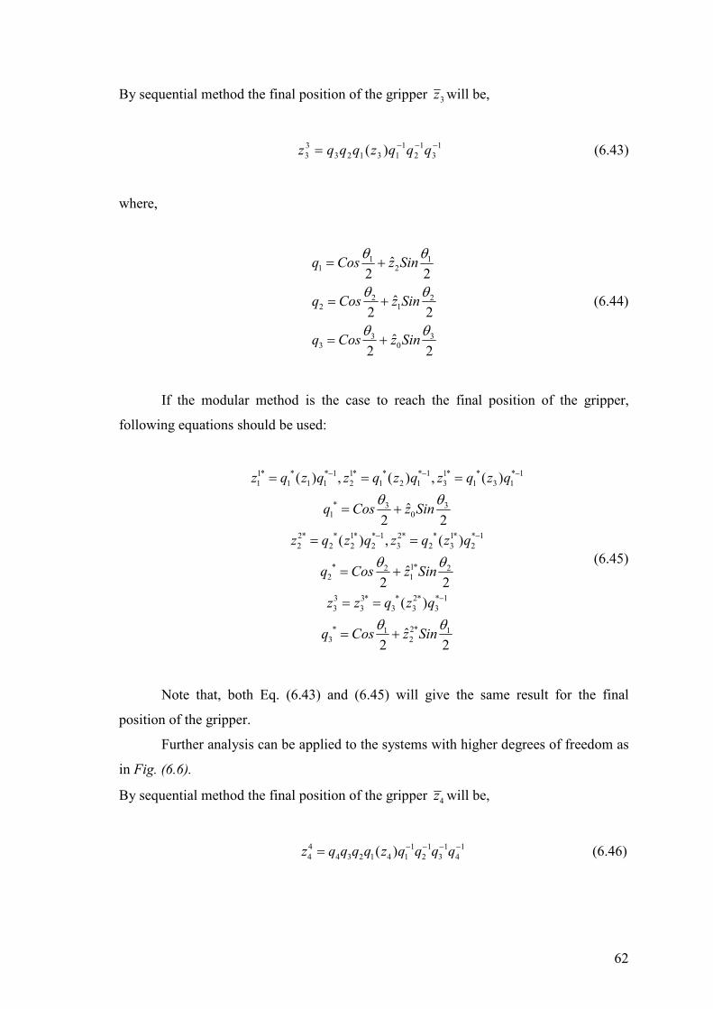
62
By sequential method the final position of the gripper 3z will be,
13
12
113123
33 )( −−−= qqqzqqqz (6.43)
where,
1 11 2
2 22 1
3 33 0
ˆ2 2
ˆ2 2
ˆ2 2
q Cos z Sin
q Cos z Sin
q Cos z Sin
θ θ
θ θ
θ θ
= +
= +
= +
(6.44)
If the modular method is the case to reach the final position of the gripper,
following equations should be used:
1* * * 1 1* * * 1 1* * * 11 1 1 1 2 1 2 1 3 1 3 1
* 3 31 0
2* * 1* * 1 2* * 1* * 12 2 2 2 3 2 3 2
* 1*2 22 1
3 3* * 2* * 13 3 3 3 3
* 2*1 13 2
( ) , ( ) , ( )
ˆ2 2
( ) , ( )
ˆ2 2
( )
ˆ2 2
z q z q z q z q z q z q
q Cos z Sin
z q z q z q z q
q Cos z Sin
z z q z q
q Cos z Sin
θ θ
θ θ
θ θ
− − −
− −
−
= = =
= +
= =
= +
= =
= +
(6.45)
Note that, both Eq. (6.43) and (6.45) will give the same result for the final
position of the gripper.
Further analysis can be applied to the systems with higher degrees of freedom as
in Fig. (6.6).
By sequential method the final position of the gripper 4z will be,
4 1 1 1 14 4 3 2 1 4 1 2 3 4( )z q q q q z q q q q− − − −= (6.46)

63
Figure 6.6. Position Vectors of a Spherical Serial Wrist with 4-DoF
where,
1 11 3
2 22 2
3 33 1
4 44 0
ˆ2 2
ˆ2 2
ˆ2 2
ˆ2 2
q Cos z Sin
q Cos z Sin
q Cos z Sin
q Cos z Sin
θ θ
θ θ
θ θ
θ θ
= +
= +
= +
= +
(6.47)
If the modular method is the case to reach the final position of the gripper,
following equations should be used:
1* * * 1 1* * * 11 1 1 1 2 1 2 1
1* * * 1 1* * * 1 * 4 43 1 3 1 4 1 4 1 1 0
( ) , ( )
ˆ( ) , ( ) ,2 2
z q z q z q z q
z q z q z q z q q Cos z Sinθ θ
− −
− −
= =
= = = + (6.48a)

64
2* * 1* * 1 2* * 1* * 1 2* * 1* * 12 2 2 2 3 2 3 2 4 2 4 2
* 1*3 32 1
3* * 2* * 1 3* * 2* * 13 3 3 3 4 3 4 3
* 2*2 23 2
4 4* * 3* * 14 4 3 4 3
* 3*3 34 3
( ) , ( ) , ( )
ˆ2 2
( ) , ( )
ˆ2 2
( )
ˆ2 2
z q z q z q z q z q z q
q Cos z Sin
z q z q z q z q
q Cos z Sin
z z q z q
q Cos z Sin
θ θ
θ θ
θ θ
− − −
− −
−
= = =
= +
= =
= +
= =
= +
(6.48b)
Again, note that, both Eq. (6.46) and (6.48) will give the same result for the final
position of the gripper.
6.5. Workspaces of the Spherical Wrists
By using the computed equations of the 2-DoF, 3-DoF and 4-DoF spherical
wrists, the workspaces of the grippers are analysed Fig. (6.7), (6.8), and (6.9).
Figure 6.7. Workspace of a Spherical Serial Wrist with 2-DoF

65
Figure 6.8. Workspace of a Spherical Serial Wrist with 3-DoF
Figure 6.9. Workspace of a Spherical Serial Wrist with 4-DoF

66
CHAPTER 7
GEOMETRICAL ANALYSIS OF THE HUMAN
CLAVICLE AND ELBOW MANIPULATOR
7.1. Geometrical Analysis of Spatial 3-DoF Orientation Mechanism in
λ=6
Now, the first part, proposed for the clavicle, of the new manipulator design with
variable general constraints that mimics human shoulder, elbow and wrist complex will
be analysed with respect to the geometrical approach Fig. (7.1-7.2).
Figure 7.1. Orientation Platform (Red) of the New Manipulator Design
Figure 7.2. Orientation Platform (Closed View)

67
Eq.(7.1) shows the simple equation of a sphere with radius “r” whose center is
fixed at the origin Fig.(7.3) and the Eq. (7.2) shows the case when the center is away
from the origin 1 1 1( , , )x y z Fig. (7.3).
2 2 2 2x y z r+ + = (7.1)
2 2 2 21 1 1( ) ( ) ( )x x y y z z r− + − + − = (7.2)
Figure 7.3. Sphere with Radius “r” whose Center is Fixed at the Origin
Figure 7.4. Sphere with Radius “r” whose Center is Away from the Origin

68
Now let us consider the generalized mechanism in Fig. (7.5). We will set the
origin point of the Cartesian coordinate system as the rotation center of the mechanism
where z axis is perpendicular to the upper platform in the initial configuration.
To start to analyse the workspace of the first point 1D we will draw the vector
from the origin to the point 1D . From this point we can describe the workspace of 1r as a
sphere “A” whose equation is,
1 1 1
2 2 2 2
1D D Dx y z r+ + = (7.3)
In second operation, we will pass to the leg 1d . By using the constructional
parameters we can easily find the coordinates of 1O 1 1 1( , , )x y z . Due to the limitation of
the leg 1d the work space of the vector will be the volume between the spheres B and C.
We can show this in equation as,
1 1 1
2 2 2 2
1 1 1 1
1 1min 1max
( ) ( ) ( )D D Dx x y y z z d
d d d
− + − + − =
= → (7.4)
By the same analogy, we can write other 4 equations for the other legs,
2 2 2
2 2 2 2
2D D Dx y z r+ + = (7.5)
2 2 2
2 2 2 2
2 2 2 2
2 2min 2max
( ) ( ) ( )D D Dx x y y z z d
d d d
− + − + − =
= → (7.6)
3 3 3
2 2 2 2
3D D Dx y z r+ + = (7.7)
3 3 3
2 2 2 2
3 3 3 3
3 3min 3max
( ) ( ) ( )D D Dx x y y z z d
d d d
− + − + − =
= → (7.8)

69
Figure 7.5. Generalized Orientation Mechanism
At this point we have 6 equations with 9 unknowns, of which 6 of them are
independent and 3 of them are dependent with respect to the Eq. (7.3), (7.5) and (7.7),
remaining 3 equations comes from the construction parameters of the upper platform
Fig. (7.6).

70
Figure 7.6. Construction Parameters of Upper Platform (a, b, c)
By using the fixed lengths, a, b, and c,
1 2 1 2 1 2
2 2 2 2( ) ( ) ( )D D D D D Dx x y y z z a− + − + − = (7.9)
2 3 2 3 2 3
2 2 2 2( ) ( ) ( )D D D D D Dx x y y z z c− + − + − = (7.10)
1 3 1 3 1 3
2 2 2 2( ) ( ) ( )D D D D D Dx x y y z z b− + − + − = (7.11)
Now from the 9 equations Eq. (7.3÷7.11), we can easily start to compute the
unknowns , ,i i iD D Dx y z (i=1, 2, 3).
From the Eq. (7.3), (7.5) and (7.7), we will get,
1 1 1
2 2 2
3 3 3
21
22
23
D D D
D D D
D D D
z r x y
z r x y
z r x y
= ± − −
= ± − −
= ± − −
(7.12)
by using the transformations in Eq. (7.13), equation sets can be rewritten as,
1
1
1
1
1
1
D
D
D
x x
y y
z z
=
=
=
%
%
%
(7.13)

71
2 2 2 2
1 1 1 1 1 1 1
2 2 2 2
2 2 2 2 2 2 2
2 2 2 2
3 3 3 3 3 3 3
2 2 2 2
1 2 1 2 1 2
2 2 2 2
1 3 1 3 1 3
2 2
3 2 3 2 3 2
( ) ( ) ( )
( ) ( ) ( )
( ) ( ) ( )
( ) ( ) ( )
( ) ( ) ( )
( ) ( ) ( )
x x y y z z d
x x y y z z d
x x y y z z d
x x y y z z a
x x y y z z b
x x y y z z
− + − + − =
− + − + − =
− + − + − =
− + − + − =
− + − + − =
− + − + −
% % %
% % %
% % %
% % % % % %
% % % % % %
% % % % % %2 2
c=
(7.14)
expanding the equations,
2 2 2 2 2 2 2
1 1 1 1 1 1 1 1 1 1 1 1 1
2 2 2 2 2 2 2
2 2 2 2 2 2 2 2 2 2 2 2 2
2 2 2 2 2 2 2
3 3 3 3 3 3 1 1 1 1 1 1 3
2 2 2 2 2 2
1 1 1 2 2 2 1 2 1 2
2 2 2
2 2 2
2 2 2
2 2 2
x y z x y z x x y y z z d
x y z x y z x x y y z z d
x y z x y z x x y y z z d
x y z x y z x x y y
+ + + + + − − − =
+ + + + + − − − =
+ + + + + − − − =
+ + + + + − − −
% % % %% %
% % % %% %
% % % %% %
% % % % % % % %% %2
1 2
2 2 2 2 2 2 2
1 1 1 3 3 3 1 3 1 3 1 3
2 2 2 2 2 2 2
2 2 2 3 3 3 2 3 2 3 2 3
2 2 2
2 2 2
z z a
x y z x y z x x y y z z b
x y z x y z x x y y z z c
=
+ + + + + − − − =
+ + + + + − − − =
% %
% % % % % % % %% % % %
% % % % % % % %% % % %
(7.15)
using Eq. (7.3), (7.5) and (7.7), and arranging the terms,
2 2 2 2 21 1 1 1 1 1 1 1 1 1 1
2 2 2 2 22 2 2 2 2 2 2 2 2 2 2
2 2 2 2 23 3 3 3 3 3 3 3 3 3 3
2 2 21 2 1 2 1 2 1 2
2 2 21 3 1 3 1 3 1 3
1( )
21( )
21( )
21( )
21( )
2
x x y y z z d r x y z
x x y y z z d r x y z
x x y y z z d r x y z
x x y y z z a r r
x x y y z z b r r
x
+ + = − + + + +
+ + = − + + + +
+ + = − + + + +
+ + = − + +
+ + = − + +
% % %
% % %
% % %
% % % % % %
% % % % % %
%2 2 2
2 3 2 3 2 3 2 3
1( )
2x y y z z c r r+ + = − + +% % % % %
(7.16)
For simplifying purposes, new parameters can be used as,

72
2 2 2 2 21 1 1 1 1
2 2 2 2 22 2 2 2 2
2 2 2 2 23 3 3 3 3
2 2 21 1 2
2 2 22 1 3
2 2 23 2 3
1( )
21( )
21( )
21( )
21( )
21( )
2
p d r x y z
q d r x y z
t d r x y z
s a r r
s b r r
s c r r
= − + + + +
= − + + + +
= − + + + +
= − + +
= − + +
= − + +
(7.17)
and using equation set (7.12),
2
1 1 1 1 1 1 1 1
2
2 2 2 2 2 2 2 2
2
3 3 3 3 3 3 3 3
2 2
1 1 1 2 2 2 1 1 2 1 2
2 2
1 1 1 3 3 3 2 1 3 1 3
2 2
2 2 2 3
( )
( )
( )
( )( )
( )( )
( )(
r x y z p x x y y
r x y z q x x y y
r x y z t x x y y
r x y r x y s x x y y
r x y r x y s x x y y
r x y r
± − − = − −
± − − = − −
± − − = − −
± − − ± − − = − −
± − − ± − − = − −
± − − ± −
% % % %
% % % %
% % % %
% % % % % % % %
% % % % % % % %
% %3 3 3 2 3 2 3)x y s x x y y− = − −% % % % % %
(7.18)
Squaring both sides and arranging,
2 2 2 2 2 2 2 2 21 1 1 1 1 1 1 1 1 1 1 1 1 1 1 1
2 2 2 2 2 2 2 2 22 2 2 2 2 2 2 2 2 2 2 2 2 2 2 2
2 2 2 2 2 23 3 3 3 3 3 3 3 3 3
( ) ( ) (2 ) (2 ) ( 2 )
( ) ( ) (2 ) (2 ) ( 2 )
( ) ( ) (2 ) (2 )
x z x y z y x px y py x y x y p z r
x z x y z y x qx y qy x y x y q z r
x z x y z y x tx y ty x
− − + − − + + + − = −
− − + − − + + + − = −
− − + − − + + +
% % % % % %
% % % % % %
% % % % %2 2 2
3 3 3 3 3 3
2 2 2 2 2 2 2 2 2 2 2 21 2 1 2 2 1 2 1 1 2 1 2 1 2 1 1 2 1
2 2 21 2 1 2 1 1 2
2 2 2 2 2 2 2 2 2 2 2 21 3 1 3 3 1 3 1 1 3 1 3 1
( 2 )
( ) ( ) ( ) ( ) (2 ) (2 )
( 2)
( ) ( ) ( ) ( )
y x y t z r
x r y r x r y r x y y x xx s y y s
xx y y s r r
x r y r x r y r x y y x x
− = −
− + − + − + − + + + +
+ − = −
− + − + − + − + + +
%
% % % % % % % % % % % %
% % % %
% % % % % % % % %3 1 1 3 1
2 2 21 3 1 3 2 1 3
2 2 2 2 2 2 2 2 2 2 2 22 3 2 3 3 2 3 2 2 3 2 3 2 3 1 2 3 2
2 2 22 3 2 3 2 2 3
(2 ) (2 )
( 2)
( ) ( ) ( ) ( ) (2 ) (2 )
( 2)
x s y y s
xx y y s r r
x r y r x r y r x y y x x x s y y s
x x y y s r r
+
+ − = −
− + − + − + − + + + +
+ − = −
% % %
% % % %
% % % % % % % % % % % %
% % % %
(7.19)

73
and, in the end, after the combinations of the known values, our final equation sets, that
has 6 independent variables will be,
2 21 1 2 1 3 1 4 1 5 1 1
2 21 2 2 2 3 2 4 2 5 2 2
2 21 3 2 3 3 3 4 3 5 3 3
2 2 2 2 2 2 2 21 1 2 1 3 2 4 2 5 1 2 6 1 2 7 1 2 8 1 2
9 1 2 1 2
21 1
Ax A y A x A y A x y A
B x B y B x B y B x y B
C x C y C x C y C x y C
D x D y D x D y D x y D y x D x x D y y
D x x y y D
E x E
+ + + + =
+ + + + =
+ + + + =
+ + + + + + +
+ =
+
% % % % % %
% % % % % %
% % % % % %
% % % % % % % % % % % %
% % % %
%2 2 2 2 2 2 2
2 1 3 3 4 3 5 1 3 6 1 3 7 1 3 8 1 3
9 1 3 1 3
2 2 2 2 2 2 2 21 2 2 2 3 3 4 3 5 2 3 6 2 3 7 2 3 8 2 3
9 2 3 2 3
y E x E y E x y E y x E x x E y y
E x x y y E
F x F y F x F y F x y F y x F x x F y y
F x x y y F
+ + + + + +
+ =
+ + + + + + +
+ =
% % % % % % % % % % %
% % % %
% % % % % % % % % % % %
% % % %
(7.20)
As we have six independent equations and six unknowns, there exists a unique
solution for the position of the platform with respect to the given parameters. So that,
solving the Eq. (7.20) by numerical methods and get the positions of the corners, any
position and orientation of the center of the orientation platform can be found by using
the input parameters.
7.2. Geometrical Analysis of Spatial 2-DoF Orientation Mechanism in
λ=6
Unlike the 3-DoF orientation mechanism, geometric analysis of the manipulator
proposed for the ankle joint is relatively simple Fig (7.7) and (7.8), as the control of the
platform is carried out by two actuators separately.
In Fig. (7.9), on the closed view of the platform base, two revolute actuators A,
and B can easily be seen. As it is mentioned, revolute actuator A is responsible for the
position of the platform and the other revolute actuator is responsible for the orientation
of the platform.
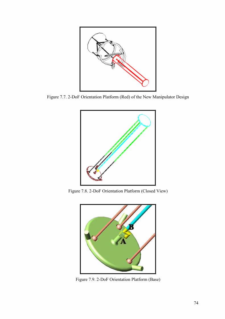
74
Figure 7.7. 2-DoF Orientation Platform (Red) of the New Manipulator Design
Figure 7.8. 2-DoF Orientation Platform (Closed View)
Figure 7.9. 2-DoF Orientation Platform (Base)

75
Figure 7.10. Generalized 2-DoF Orientation Platform
Now, consider the manipulator in Fig (7.10) will be rotated by the angle θ
around z axis by using revolute actuator A in clock wise direction, and rotated by the
angle α around the floating y axis. Note that in this operation, the platform of the
shoulder is taken as a fixed frame. Due to the fact that, the center of the upper platform
(D), will always remain on the circle with radius r, the last position of the platform will
be,
( )
( )
0
x rSin
y rCos
z
θ
θ
=
=
= (7.21)
and the final orientation will be the angle α.

76
Let us now prove the positions by the help of the rotation matrices. As seen in
Fig. (7.10) the first position of the center point of the upper platform is D(0,r,0) and the
final position is Df(0,r,0). By using the rotational sequences,
( , ) ( , )f R z R y DD θ α= − (7.22)
Expanding and evaluating the Eq. (7.22),
( ) ( ) 0 0 0
( ) ( ) 0 0 1 0
0 0 1 0 0
0 0
0
0 0 1 0
0
C S C S
S C r
S C
C S
S C r
rS
rC
x
y
z
θ θ α α
θ θ
α α
θ θ
θ θ
θ
θ
− − −
= − −
−
−
=
=
(7.23)
So, the results of Eq. (7.23) prove the geometrical interpretation for the final
position of the platform Eq. (7.21). By using these equations any of the positions of the
platform can be computed with respect to the given parameters.

77
CHAPTER 8
CONCLUSION
It has been shown in this study that, rigid body rotations can be carried out by
using two different techniques through quaternion algebra with different quaternion
operators. The advantage is the fact that, it is very simple procedure to use quaternions
in rotation sequences when compared with the rotation matrices or other alternative
tools; thus, this means fewer operations and less computational time. Analysis of the
results through kinematics of spherical human wrist manipulators has proved that the
theory is applicable practically as well as theoretically. Also it has been shown that
sequential model is closer to the traditional motion of robot manipulators, while the new
proposed modular method is closer to the human motion of robot manipulators.
Moreover, in this study, a new structural formula for spatial parallel
manipulators having one general moving platform, working in Cartesian space with
three legs that are placed in orthogonal planes introducing simple structural groups in
subspaces λ=3, 4 and general space λ=6, and connected to actuators and to the general
moving platform is introduced. History of formulas DoF is presented as 38 equations
with the unique key controlling parameters. 9 new parallel Cartesian platform robot
manipulators are introduced by applying new mobility loop-legs equation. Structural
synthesis of serial platform manipulators and parallel Cartesian platform manipulators
are considered. Simple serial platform structural groups in subspace λ=3, and general
space λ=6 are presented along with examples.
Finally, after the type synthesis of human arm is completed with the illustrations
of the human arm, a new manipulator with variable general constraints that mimics
human shoulder, elbow and wrist complex is proposed with its structural synthesis. The
manipulator has two orientation platforms in space 6λ = and one spherical platform in
subspace 3λ = . At the end of the study, geometrical kinematic analysis of the
orientation platforms of the new manipulator design for the human arm is accomplished.

78
REFERENCES
Agrawal, V.P.,and Rao, J.S., 1987. “Fractionated freedom kinematic chains and
mechanisms”, Elsevier, IFToMM J. Mech. Mach. Theory Vol. 22, pp. 125-130.
Alizade R.I. and Kilit, Ö., 2005. “Analytical Synthesis of Function Generating Spherical
four-bar Mechanism for the Five Precision Points”, IFToMM J. Mach. and Mech.
Theory, Vol. 40, pp. 863-878.
Alizade, R.I., and Bayram, C., 2004. “Structural synthesis of parallel manipulators”,
Elsevier, IFToMM J. Mech. Mach. Theory, Vol. 39, pp. 857-870.
Alizade, R., Bayram, C., and Gezgin. E., 2006, “Structural synthesis of Serial Platform
Manipulators”, Elsevier, IFToMM J. Mech. Mach. Theory, MMT 40-129.
Alizade, R.I., 1988. “Investigation of linkage mechanisms with lower pairs from point
of view of its structure and classification”, Azerb. Poly. Inst., Baku, pp. 111-127.
Alizade, R.I., 1988. “On degree of freedom of kinematic chain”, Azerbaijan Polytech.
Inst. Automation design of mechanisms, manipulators and robots, Baku, pp.3-14.
Alizade, R.I., Hajiyev, E.T., and Sandor, G.N., 1985. “Type synthesis of spatial
mechanisms on the basis of spatial single loop structural groups”, IFToMM J. Mech.
Mach. Theory, Vol. 20, pp. 95-101.
Angales, J., 1988. “Rational Kinematics”, (Springer Verlag, New York).
Angeles, J., and Gosselin, C., 1988. “Determination du degree de liberte des chaines
cinematiques”, Trans. CSME Vol.12/4, pp. 219-226.
Antonescu, P., 1973. “Extending of structural formula of Dobrovolski to the complex
mechanisms with apparent family”, Proceedings of the SYROM, Bucharest.

79
Artobolevskii, I. I., 1935-1939. “To structure of spatial mechanisms” Vol. 10,
pp. 110-152, and “Experience of structural analysis, Structure and classification of
mechanisms” Moscow pp. 49-66.
Artobolevskii, I.I., 1939. “Structural analysis experience of mechanisms. Structure and
classification of mechanisms”, AS USSR, pp.49-66.
Assur, L.V., 1916. “Investigation of plane linkage mechanisms with lower pairs from
point of view of their structure and classification” unpublished dissertation, AS
USSR p.529.
Bagci, C. 1971. “Degrees of freedom of motion in mechanisms”, ASME J. Eng. Industry
Vol. 93, B pp. 140-148.
Baranov, G.G., 1952. “Classification, structure, kinematic and kinetostatic of
mechanisms with first order pairs”, AS USSR, Mech. Mach. Theory, Vol. 46,
pp.15-39.
Boden, H., 1962. “Zum zwanglauf genuscht raümlichebener getriebe”,
Maschinenbautechnic Vol. 11, pp. 612-615.
Bonev. I.A., and Gosselin. C., 2005. “Singularity loci of spherical parallel
mechanisms”, Proceedings of the IEEE International Conference on Robotics and
Automation, Barcelona, Spain, pp. 2968-2973.
Bosscher, P. et al. 2003. “A novel mechanism for implementing multiple collacated
spherical joints”, Proceedings of the IEEE International Conference on Robotics
and Automation, Taipei, Taiwan, pp. 336-341.
Bottema, O., and Roth, B., 1979. “Theoretical Kinematics”, North Holland.
Buchsbaym, F., 1967. “Structural classification and type synthesis of mechanisms with
multiple elements”, Ph.D Disertation, Columbia University.

80
Chebyshev, P.L., 1869. “Théorie des mécanismes connus sais le non de
parallélogrammes, 2 éme partie” Mémoires présentes a 1’Academie impériale des
sciences de Saint-Pétersbourg par divers savants.
Courant, R., Robbins, and H., Stewart, I., 1996. “What is mathematics”, (N.Y., USA,
Euler’s formula) pp. 235-240.
Crane, D., III, and Duffy, J., 1998. “Kinematic Analysis of Robot Manipulators”
(Cambridge University Press, N.Y, USA).
Davies, T.H., 1981. “Kirchoff’s circulation law applied to multi-loop kinematic chains”,
Elsevier, IFToMM J. Mech. Mach. Theory, Vol. 16, pp. 171-183.
Davies, T.H., and Crossley, F.R.E., 1966. “Structural analysis of plane linkages by
Franke’s condensed notation”, J. Mech., Vol. 1, pp. 171-183.
Djoldasbekov, Y.A., Baygunchekov, J.J., 1976. “Structural analysis one loop Assur
groups of higher class”, Kaz. Acad Sc, p. 12.
Dobrjanskyi, L., 1966. “Application of graph theory to the structural classification of
mechanisms”, Ph.D Disertation, Columbia University.
Dobrjanskyi, L., and Freudenstein, F., 1967. “Some applications of graph theory to the
structural analysis of mechanisms”, Trans. ASME J. Eng. Ind., pp. 153-158.
Dobrovolskii, V.V., 1939. “Main principles of rational classification”, AS USSR
pp. 5-48.
Dudita, F, and Diaconescu, D., 1987. “Optimizarea structurala a mecanismelor”,
Technica, Bucuresti, pp.36-45, pp. 229-254.
Encyclopedia Britannica, 1886. “Quaternions”, pp. 160-164.

81
Freudenstein, F., 1967. “The basic concepts of Polya’s theory of enumeration with
application to the structural classification of mechanisms”, J. of Mechanisms,
Vol. 3, pp. 275-290.
Freudenstein, F., and Alizade, R.I., 1975. “On the degree of freedom of mechanisms
with variable general constraint”, IV World IFToMM Congress, England, pp. 51-56.
Gogu, G., 2005. “Mobility of mechanisms: a critical review”, Elsevier, IFToMM J.
Mech. Mach. Theory, Vol. 40, pp. 1068-1097.
Gokhman, Kh.I., 1889. “Equation for mobility definition and solution of mechanism
classification” Odessa.
Gosselin, C., 1994. “The agile eye: A high performance 3DoF camera orienting device”,
Proceedings of the IEEE International Conference on Robotics and Automation,
San Diego, CA, pp. 781-786.
Gronowicz, A., 1981. “Identifizierungs-Methode der Zwanglaufbedingungen von
kinematischen ketten”, Elsevier, IFToMM J. Mech. Mach. Theory, Vol. 16,
pp. 127-135.
Grübler, M., 1883, 1885. “Allgenmeine Eigenschaften der swanglaufigen ebeden
kinematischen ketten part I Zivilingenieur 29” 167-200, “part II Verh. Ver. Bef.
Gew. 64” pp. 179-223.
Hamilton, W.R., 1866.” Elements of Quaternions”, London.
Herve, J.M., 1978. “Analyse structurelle des mécanismes par groupe des
déplacements”, Mech. Mach. Theory, Vol. 13., pp. 437-450.
Huang, Z., and Li, Q.C., 2003. “Type synthesis of symmetrical lower-mobility parallel
mechanisms using the constraint-synthesis method”, J. Robotics Res. Vol. 22,
pp. 59-79.

82
Hunt, K.H., 1978. “Kinematic geometry of mechanisms”, (Oxford Univ. Press, Oxford).
Hwang, W.M., and Hwang, Y.W. 1986. “Computer-aided structural synthesis of
mechanisms”, Trans. ASME Vol. 108, pp. 392-398.
Jin, Q. , and Yang, T., 2001. “Structure synthesis of a class of five DoF (three
translation and two rotation) parallel robot mechanisms based on single-opened-
chain units”, Proceedings of ASME 27th design Automotion conference, Pittsburgh,
DETC/DAC-21153.
Jin, Q. , and Yang, T., 2002. “Structure synthesis of a class of three DoF translational
parallel robotic mechanisms based on the units single-opened-chain”, Chinese J. of
Mech. Eng. Vol. 38.
Koenigs, G., 1905. “Introduction a une théorie nouvelle des mécanismes” (Librairie
Scientifique A. Hermann, Paris) pp. 27-28.
Kojevnikov, S.N., 1979. “Foundation of structural synthesis of mechanisms”, Kiyev,
p.229.
Kolchin, N.I., 1932-1934. “Applied mechanic in problems” (Issue I-IV, Peterburg)
Kolchin, N.I., 1960. “Experience structure of widening structural classification of
mechanisms and base to its structural table of mechanisms”, Analysis and Synthesis
of Mechanisms, Moscow, pp. 85-97.
Kutzbach, K., 1929. “Mechanische leitungsverzweigung, ihre gezetze und
anwendungen, Maschinenbau” Betrieb Vol. 8, pp. 710-716.
Larochelle, P., 2000. “Approximate motion Synthesis via Parametric Constraint
Manifold Fitting” Advances in Robot Kinematics, (Kluwer Acad. Publ., Dordrecht).
Malushev, A.P., 1923. “Analysis and synthesis of mechanisms from point of view of
their structure” Tomsk, p. 91.

83
Malushev, A.P., 1929. “Analysis and synthesis of mechanisms from point of view of
their structure”, Tomsk, p. 78.
Manolescu, N. 1968. “For a united point of view in the study of the structural analysis
of kinematic chains and mechanisms”, J. Mech. Vol. 3, pp. 149-169.
Manolescu, N.I., 1973. “A method based on Baranov trusses and using graph theory to
find the set of planar jointed kinematic chains and mechanisms”, Elsevier, IFToMM
J. Mech. Mach. Theory Vol. 1, pp. 3-22.
McCarthy, J.M., 1990. “An Introduction to Theoretical Kinematics”, (MIT Press).
McCarthy, J.M., 2000. “Geometric design of linkages”, (Springer-Verlag, N.Y.), p.320.
Moroshkin, U.F., 1958. “Geometry problems of complex kinematic chains”, AS USSR
Vol. 119, pp. 38-41.
Mueller, R., 1920. “Die zwanglanfigkeit kinematische ketten” unpublished dissertation
(as quoted in Federhofer, K., 1932. “Graphische kinematic and kinetostatic”
(Springer, Berlin))
Nixravesh, R.A., Wehage and Kwan, O.K., 1985. “Euler Parameters in Computational
Kinematics and Dynamics”. Part 1, ASME J. Mech. Trans., Aut. Des., Vol. 107,
pp. 358-365.
Okada, M., Nakamura, Y., and Hoshino, S. “Design of programmable passive
complience shoulder mechanism”, Dept. Of Mechano-Informatics, Univ. of Tokyo.
Okada, M., Nakamura, Y., and Hoshino, S. “Development of the cybernetic shoulder- A
three DoF mechanism that imitates biological shoulder motion”, Dept. Of Mechano-
Informatics, Univ. of Tokyo.
Ozol, O.G, 1962. “A new structural formula for mechanisms and its theoretical and
practical importance”, Latv. Agric. Acad. Vol. 11, pp. 113-129.

84
Ozol, O.G., 1963. “Expansion of structural theory and classification plane mechanisms
with lower pairs”, Latv. Acrycult. Acad, Vol. 13, pp. 71-91.
Paul, B, 1960. “A unified criterion for the degree of constraint of plane kinematic
chains”, J. Appl. Mechanics Vol. 27, pp. 196-200.
Porteous, I.R., 1921. “Topological Geometry”, (Cambridge University Press,
Cambridge, U.K).
Rao, A.C., and Deshmukh, P.B., 1995. “Computer aided structural synthesis of planar
kinematicchains with simple joints”, Elsevier, IFToMM J. Mech. Mach. Theory
Vol. 30, pp. 1193-1215.
Rico-Martinez, J.M. and Gallardo-Alvarado, J., 2000. “A simple method for the
determination of angular velocity and acceleration of a spherical motion through
quaternions” Nederlands, Meccanica Vol. 35, pp. 111-118.
Rössner, W., 1961. “Zur strukturellen ordnung der getriebe” (Wissenschaft. Tech.
Univ., Dresden), Vol. 10, pp. 1101-1115.
Shen, H., Yang, T., and Ma, L. 2005. “Synthesis and structure analysis of kinematic
structures of 6 DoF parallel robotic mechanisms”, Elsevier, IFToMM J. Mech.
Mach. Theory.
Sohn, W.J., and Freudenstein, F., 1986. “An application of dual graphs to the automatic
generation of kinematic structures of mechanisms”, Trans. ASME, Vol. 108,
pp. 392-398.
Somov, P.O., and Chen, J.P., 1987. “On the DoF of kinematic chains” pp. 443-447
Stanisic M.M. et al., 2001. “A dextereous humanoid shoulder mechanism”, Journal of
robotic systems, Vol. 18, pp. 737-745.

85
Sylvester, J.J., 1874. “On recent discoveries in mechanical conversion of motion” Proc.
Roy. Inst. Great Britain, Vol. 7/5, pp. 179-198.
Voinea, R., and Atanasiu, M., 1959 “Contributions a la theorie geometrigue des vis”,
(Bull. Inst. Politech. Bucuresti, XXI).
Voinea, R., and Atanasiu, M., 1960. “Contribution a l’etude de la structure des chaines
cinematiques”, Bulrtinul Institutului Pol., Bucharesti, 21-1.
Waldron, K.J., 1966. “The constraint analysis of mechanisms”, J. Mech. Vol. 1,
pp. 101-114.
WEB_1,2005. “A history of Clifford Algebras”, 03/04/2005.
(http://members.fortunecity.com/jonhays/clifhistory.htm)
Wu. G. et al. 2004. “ISB recommendation on definitions of joint coordinate systems of
various joints for the reporting of human joint motion-Part II: shoulder, elbow, wrist
and hand”, Journal of Biomechanics, Vol. 38. pp. 981-992.
Xin-Jun Liu, Jinsong Wang and Fang Gao, 2003. “Workspace Atlases for the Design of
Spherical 3-DoF Serial Wrists”, J. of Intelligent and Robotic Systems Vol. 36, pp.
389-405.
Yang, T., 1983. “Structural analysis and number synthesis of spatial mechanisms”, Sixth
World Congress on Theory Mach. and Mech., New Delhi, India, pp. 280-283.
Yang, T., 1985. “Structural synthesis of spatial multi loop chains with variable over
constraints”, The Fourth IFToMM Symp., Bucharest, Romania, Vol. 11,
pp. 447-456.

86
APPENDIX A
RESULT OF THE EQUATIONS
12
111123 )( −−= qqrqqr AND
2 1 12 2 1 2 1 2( )r q q r q q• • •− •−=
[ ], , ,Quaternion a b c d
[ ]0a =
[ ]
2
21 1
1 2 2 2 2 2 2 2( 2 2 ((1 ) 2 ( ))1 2 3 1 2 1 3 1 2 3 1 2 32
2( 2 2 ) ) (2 2 23 2 1 3 2 1 2 3 2 3 2 3 1 3
2 2 2 2 222 3 3 3 2 1 2 2 2 3 2 2
2Cos x m x m x m x m m y m m z m m m x m m y m z
Cos m y m z Sin Sin m m n x m m n x m m n y n y m n y
m n y m n y n z m n z m n z m n z m m
b
θ θ
θ
θ
+ − − + + + − + + − +
+ − + + − + − + −
+ + − − + −
=
2
1
1
2( ( 2 2 )3 3 1 3 2 2 3 3 3 3
2 2 2( ) ( ) ( 2 2 2 )) 2(2 3 2 1 3 2 2 3 2 2 3 2 3 2 3 3 2 2
2 2 2 2 2 2 2 2( )) ) ( 43 3 1 2 3 1 1 1 2 1 3 1 1 2 1 22
n z m m n x m n x n y m n y
n z m n z m n y n z m n y n z m m n y m n y m n z Cos m n x
m n x m n y n z Sin Sin n x m n x m n x m n x m m n n x
θ
θθ
+ − + − −
+ − + − + + + + − + + −
+ − + + + − − +
22
2 2 2 2 2 2 2 2 2 2 2 2 24 2 2 21 2 2 2 1 3 1 3 3 1 3 2 3 3 3 1 2 1 1 2 1 1 2
2 2 2 2 2 22 2 2 4 2 2 4 22 1 2 3 1 2 1 2 2 2 3 1 3 1 2 3 1 3 1 2 3 1 2 1 3 2
2 22 2 2 21 3 1 1 3 2 1 3
n x
m n x m n x m m n n x n x m n x m n x m n x m m n y n n y m n n y
m n n y m n n y m m n y m m n n y m m n y m m n z m m n n z m m n z
n n z m n n z m n n z m
− −
+ + − − + + + + − +
− − + − + + − +
− − +
1
2 2 2 2 2 22 ( (( 1 ) 2 ( ))3 1 3 1 3 3 1 1 2 3 1 2 3
2 2 2 2 2 2 2( )(( 1 ) 2 ( )) 2 ( 2 ( ) (2 3 1 2 3 1 2 3 1 1 2 2 3 3 2 2 3
2 2 22 ) ( 2 ) ( ))) 2( ( 22 3 3 2 3 2 3 1 2 3 3 1 2
n n z m m n z n m m m x m m y m z
n n m m m x m m y m z n m m n m n x n y m y m y
m m z n m m y z m z m z m n y n z Cos m n nθ
− − − + − − + +
− + − + − − + + − − + + − +
− + − + + − + + − −
1
2 2 2( ) )1 2 3
2 2 22 ( ) (2 ( ) )) ))1 1 3 2 2 1 3 1 2 3
x n y n n y
m n n y n z m n n x n z n n z Sin θ
+ − +
+ − + + − + +

87
[ ]
[ ] [ ]
2 2 2 22 1 3 1 3 1 3 2 3 3 3 2 3 1 1 2 3 1 1 1
2 2 2 2 2 2 22 1 3 1 1 3 3 2 3 3 1 2 3 2 3 1 3 1
1 3 1 2 3 3 3 1 2 1 1 1 1
1( (2 2 2
2
2 ( (1 ) ( 2 ) ( )
2 ( )) 2 2
Sin m m n x n x m n x m n x m n x m m n y m m n y n z m n z
m n z m n z m m n z m m n x n m m y z m z m z m n x n z
m m n x m n y m n z Cos m n xSin m n y
c
θ
θ θ
− − − + + + − + − −
+ − + − + + + − + + − + +
+ − + + − +
=
[ ] [ ]
[ ]
[ ] [ ]
1 3 3 1
2 2 2 2 222 3 1 1 2 1 2 3 2 3 1 2 1
2 2 2 222 3 2 3 1 3 1 1 1 2 1 1 2
2 2 21 1 2 2 1 2 3 1 2 1 2
2
2 ) (2 2 ( 22
2 ) 2( ) ) ( 2 22
2 2 2 2
Sin m n ySin
m n zSin Cos m m x y m y m y m y m m z m m x y m y
m y m y m m z Cos m x m z Sin Sin m m n x n n x
m n n x m n n x m n n x m n n
θ θ
θθ
θθ θ
+ −
+ + − + − + + − + + −
+ − + − + − + +
− − + 2 2 2 2 2 2 22 1 3 2 3 1 2 3 1 1 1 2 1
2 2 2 2 2 2 2 2 2 2 2 2 2 23 1 1 2 1 2 2 1 2 2 2 3 2 2 3 2 3 3 1 3 2 3
2 2 2 2 2 2 23 3 2 3 1 1 3 1 2 2 3 2 2 3 1 2 3 2 2 3 3 2 3
4 2
4 4
2 4 2 2 2 2 2
x m m n n x m n n x n y m n y m n y
m n y m m n n y n y m n y m n y m n y m m n n y n y m n y m n y
m n y m m n z m m n n z m m n z n n z m n n z m n n z m n n
+ − − + −
+ + + − + − + − + − +
− + + + − − +2 2 2 2 2 2 2 2 2 2 2 2 2
2 3 3 2 3 1 2 2 2 2 3 2 2 3 2 3 3 2 3 3 3
2 2 2 2 2 2 22 3 2 2 3 2 2 3 3 2 3 2 3 3 1 2 3 2 3
2 2 2 21 1 2 1 2 3 2 3 1 2 1
2 ( 2(1 ) 4
2 2 2 2 2 ( 2 )
(2 2 ) ( 2 (
z
m m n z m m n n x n y m n y m n y m m n n y n y m n y m n y
m m n z n n z m n n z m n n z m m n z n y m y m y m m z
m n n x n y n y n y n n z m m n
−
− − + + − + − + + − +
+ − − + − + − + − +
+ − + − + −
[ ][ ]
2 2 22 3 1 2 3 2 3 1
2 2 2 2 2 21 3 1 2 3 1 2 2 2 3 1 1 2 3 2 1 3
1
2 ) 4 ( )))
2( ( ( ) 2 ) 2 ( ) ( 2 ( ) ))
))
x n x n x n n y m n n x n z
Cos m n x n n x n n y m n n x n z m n n y n z n n z
Sin
θ
θ
− + − + +
− + − + + + − + − + − +
[ ] [ ] [ ]
2 2 2 2 2 2 221 3 2 3 1 2 3 1 3 2 3 1 2 3
2 2 2 21 2 1 1 2 1 2 1 2 1 2 2 2 3 2 1 1 1
2 22 1 3 1 1 2 2 2 3 1 1 3 2
1( (2 2 ( 2 2 )
2 2
( 2 2 ) ) (2
2 2 2
Cos m m x m m y z m z m z m z m m x m m y z m z m z m z
Cos m x m y Sin Sin m m n x n x m n x m n x m n x n y m n y
m n y m n y m m n y m m n z m m n z
d
θ
θ θ θ
+ + − − + + − − + + + −
+ − + + − − + + + −
+ − − + − +
=
[ ]
2 2 22 3 2 1 2 1 1
2 22 3 2 3 1 2 1 2 2 3 2 1 3 1 1 3 2 1
2 2 2 2 221 1 1 2 1 1 1 3 1 1 3 2 1 3 1 1 3 2 1
( (1 ) ( ) (
2 ) ( 2 2 2 )) 2 [ ] 2 [ ]
2 [ ] 2 [ ]) ( 2 2 2 2 22
m m n x m n x n y n y
m y m y m m z m m n x m n y m n z Cos m n xSin m n ySin
m n zSin m n zSin Sin m m n x m m n x n n x m n n x m n
θ θ θ
θθ θ
− + + + + + −
+ − + − + + + + −
− + − − + + − 3
2 2 2 2 23 1 3 1 2 2 3 1 3 3 2 3 1 2 3 2 1 2 1 3 2 3 1 2 3
2 2 2 2 2 2 2 2 2 2 2 2 2 2 2 2 22 2 3 3 2 3 2 3 3 1 1 1 2 1 3 1 2 1 2 2 2 3 2
21 3 1 3 2 3 2 3 3 1
2 4 2 2 2 4 2 2
2 2 2
4 4
n x
m n n x m m n n x m m n x m m n y m m n y m m n n y n n y m n n y
m n n y m n n y m m n y n z m n z m n z m n z n z m n z m n z m n z
m m n n z m m n n z n z m
− + + − − + + − +
− + − + + − − + + − +
+ + − 2 2 2 2 2 2 2 2 23 2 3 3 3 2 3 1 3 2 3 2
2 2 2 2 2 2 2 2 2 2 22 3 2 2 3 3 2 3 2 3 3 2 2 2 3 3 2 3 2 3 3 2 3
2 2 2 2 2 2 2 2 23 3 1 2 3 2 3 1 1 3 2 3 1 2 3
( 2(1 ) 2
2 2 2 2 4
( 2 ) (2 2 )
n z m n z m n z m m n n x m m n y
n n y m n n y m n n y m m n y n z m n z m n z m m n n z n z m n z
m n z n m m y z m z m z m n n x n n y n z n z n z
− + − − + + − −
+ − + + + − + − − +
+ − + + − + − + + −
[ ][ ]
1 2 3 2 1
2 2 2 2 2 23 1 2 3 1 3 1 3 3 2 1 2 1 2 3 1 3
2 2 21 1 2 3 2 3 1
(4 ( )
2 ( 2 ))) 2(2 ( ) ( ( ) 2 )
( 2 )) ))
m m n n x n y
m n x n x n x n n z Cos m n n x n y m n x n n x n n z
m n y n y n y n n z Sin
θ
θ
+ + − + − − + − + + − + −
+ − +

88
APPENDIX B
Q-BASIC CODE FOR THE CREATION OF THE STRUCTURAL
GROUPS OF SERIAL PLATFORM MANIPULATORS
DO
CLS
INPUT “Select the subspace 3 or 6”, s
REDIM s(B)
REDIM c(2)
REDIM L(2)
REDIM j(2)
REDIM a(2)
REDIM B(2)
c(1)=B-1
c(2)=B
IF s=3 THEN
FOR i=1 to B
s(i)=3
NEXT i
ELSE
PRINT “Select the platform structures 3,4,5,6:”
FOR i=1 to B
PRINT “B(“;i;”):”;
INPUT “ “, s(i)
NEXT i
END IF
Jb=0
FOR i=1 to B
Jb=jb+s(i)
NEXT i
cl(1)=jb-(2*c(1))

89
cl(2)=jb-(2*c(2))
L(1)=cl(1)+c(1)-B
L(2)=cl(2)+c(2)-B
j(1)=s*L(1)
j(2)=s*L(2)
a(1)=INT((j(1)-c(1))(cl(1))
B(1)=j(1)-c(1)-(a(1)*cl(1))
a(2)=INT((j(2)-c(2))(cl(2))
B(2)=j(2)-c(2)-(a(2)*cl(2))
CLS
PRINT “Subspace or space=”;s
PRINT “Number of platforms=”;B
PRINT “Structure of platforms”;
FOR i=1 to B
PRINT s(i);
NEXT i
PRINT “*****”
PRINT “by using” ;c(1); "hinges…"
PRINT “total number of legs=”;cl(1)
PRINT “total number of joints=”;j(1)
PRINT “in each leg there should be ”;a(1);”joints”
PRINT “remaining” ;B(1) ; ” joints can be placed to any leg”
IF B>=4 THEN
PRINT “*****”
PRINT “by using” ;c(2); "hinges…"
PRINT “total number of legs=”;cl(2)
PRINT “total number of joints=”;j(2)
PRINT “in each leg there should be ”;a(2);”joints”
PRINT “remaining” ;B(2) ; ” joints can be placed to any leg”
IF (a(1)-INT((-B(2))/(B(2)+1)))>=s THEN PRINT “warning: impossible configuration”
END IF
INPUT “Do you want to exit (y/n)”,exit$
LOOP until exit$=”y”

90
APPENDIX C
MOTION ANALYSIS OF NEW CARTESIAN ROBOT
MANIPULATORS
Figure C.1. Raw Motion Analysis

91
Figure C.2. Raw Motion Analysis

92
Figure C.3. Raw Motion Analysis

93
Figure C.4. Raw Motion Analysis

94
Figure C.5. Raw Motion Analysis

95
Figure C.6. Raw Motion Analysis

96
Figure C.7. Raw Motion Analysis

97
Figure C.8. Raw Motion Analysis
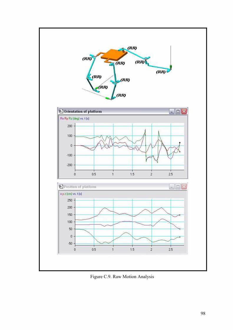
98
Figure C.9. Raw Motion Analysis