Bioinformatics for biomedicine

Gene expression data, methods of analysis

Lecture 7, 2006-10-31

Per Kraulis

http://biomedicum.ut.ee/~kraulis

Course design

1. What is bioinformatics? Basic databases and tools

2. Sequence searches: BLAST, FASTA

3. Multiple alignments, phylogenetic trees

4. Protein domains and 3D structure

5. Seminar: Sequence analysis of a favourite gene

6. More annotation, Gene Ontology and pathways

7. Gene expression data, methods of analysis

8. Seminar: Further analysis of a favourite gene

Task

• Locate protein in GO, Reactome, etc

• Wee1

• SREBP1

• Your own

Task: Wee1

• GO via– UniProt (WEE1_HUMAN)

• Protein kinase; cell cycle; nucleus

– Ensembl• Mitosis (code IEA: Inferred from Electronic

Annotation)

• Reactome– Phosphorylated by Chk1, Plk1; inactivation– Phosphorylates cyclins B1, E1, E2, A

Task: SREBP1• GO

– via UniProt• ER membrane, nuclear envelope, nucleus• Transcription factor; lipid metabolism

– Via Ensembl• Steroid metabolism (IEA)

• Reactome: nothing• KEGG: Insulin signaling pathway

– Downstream of PI3K, PIP3, PKC iota– Regulates metabolic enzymes PFK, PyK, GK

Gene activity; expression

• Gene expression = mRNA level• Proxy for gene activity

– Approximation (usually reasonable)

• Many technologies for measurement– Performance

• Absolute leve/relative change• Accuracy• Throughput (arrays vs. samples)• Predefined gene set, or identification of new genes

– Cost• Investment vs. running cost

Microarrays for gene expression

• Attach known oligonucleotides on a surface, spot by spot

• Hybridize with color-labelled sample– Relative: two samples with different color– Absolute: one single color

• Read off intensity of color in each spot– Convert to expression value for each gene– Relative change or absolute level

cDNA microarrayPat Brown’s lab, Stanford

Yeast genomeDeRisi, Iyer & BrownScience 278 (1997) 680-686

Glass slide, cDNA spotsTwo-color approach: relative change

Sample 1 (ref) is labelled green (Cy3)Sample 2 (exp) is labelled red (Cy5)

Spot colors:• Black: no mRNA; no change• Green: exp mRNA downregulated• Red: exp mRNA upregulated• Yellow: ref and exp mRNA; no change

Why not absolute values?

• C = k * Ic– C : level of mRNA– k : proportionality constant– Ic : color intensity

• Absolute value C requires k– k different for each cDNA– Calibration needed

Why relative values?

• How to avoid calibration for k ?

• Experiment relative to reference– Measure up- or down-regulation

• G = Cexp/Cref = k*Icexp/k*Icref = Icexp/Icref

• But: Equal amounts of total mRNA in the two samples (exp, ref)?

Data reduction issues

• Treatment from raw data to useful value– From spot shape/color to up/down

regulation– Similar problem in many technologies

• Many steps– Depends on microarray technology– Define spot; shape, position– Measure color intensity; background?– Handle artifacts (damaged spots, etc)

Normalization• Goal: Make data sets comparable• Microarrays

– Between colors in chip– Between chips in experiment– Between genes in different experiments

• Common approaches– Use constant gene(s); “house-keeping” genes

• Ribosomal proteins• Fundamental metabolic enzymes

– Danger: Based on assumptions!

Example analysis: Pathways

• Up/down regulation of genes

• Map onto known pathways

• Indicates changes in flows or signals

• Mechanistic information:– Verification of known data– Patterns– Interesting anomalies

• Assumes biological knowledge

Yeast: diauxic shift

• Green: anaerobic fermentation (glucose>ethanol)

• Red: aerobic respiration (ethanol>TCA cycle)

• Shows activation/ deactivation of pathways

• Behaviour of gene copies

DeRisi, Iyer & BrownScience 278 (1997) 680-686

Clustering 1

• Groups according to some property

• Computational– Measure of relationship; distance(i,j)– Many algorithms to form groups

• Powerful data analysis technique– Always some assumption on type of groups– No single optimal clustering method

Clustering 2

• A set of data points

• Two dimensions (x, y)

• How form groups?

All includedRoundness

TightnessRoundness

All includedAny shape

Clustering 3

• Depends on previous knowledge– What groups are expected?– How measure when assumptions violated?

Hierarchical How notice problem?

Clustering 4

• Hierarchical clustering– Common in gene expression analysis– Useful, but not necessary

• There is no intrinsic biological reason!

• Possible problems– Sensitive to minor errors– At what level “natural” clusters?– Hard to detect “strangely shaped” clusters

More than 2 dimensions

• More than one treatment– Ref + exp1 + exp2 + exp3 +…

• Time course experiment– Ref(t0), exp (t1), exp(t2), …

• Add other parameters– Anything of interest: pI, Mw,…

• Very common, and very useful

Scaling problem

• How to compare different dimensions?– Expression value, pI, Mw,…– Distance functions require scaling

• Making values comparable

• Possible approaches– Weights: Specific to each problem– Recalculation: Statistical

• Same average• Same standard deviation

Clustering in many dimensions

• Can be generalized into N dimensions

• Each point a vector (si, sj, …sn)

• Distance between two points– Many possible functions; also called “metric”

• Euclidean: d = sqrt(di2 + dj

2 + …dn2)

• Manhattan: d = |di | + |dj| + … |dn|

• Correlation: similar “tendency” for values s

Example: Hierarchical clustering

• 12 values per gene– Time course, 0-24 hrs

• Clustering– Correlation coefficient metric– Hierarchical; dendrogram– No cutoff level– No test of significance

Eisen et alPNAS 95 (1998) 14863-14868

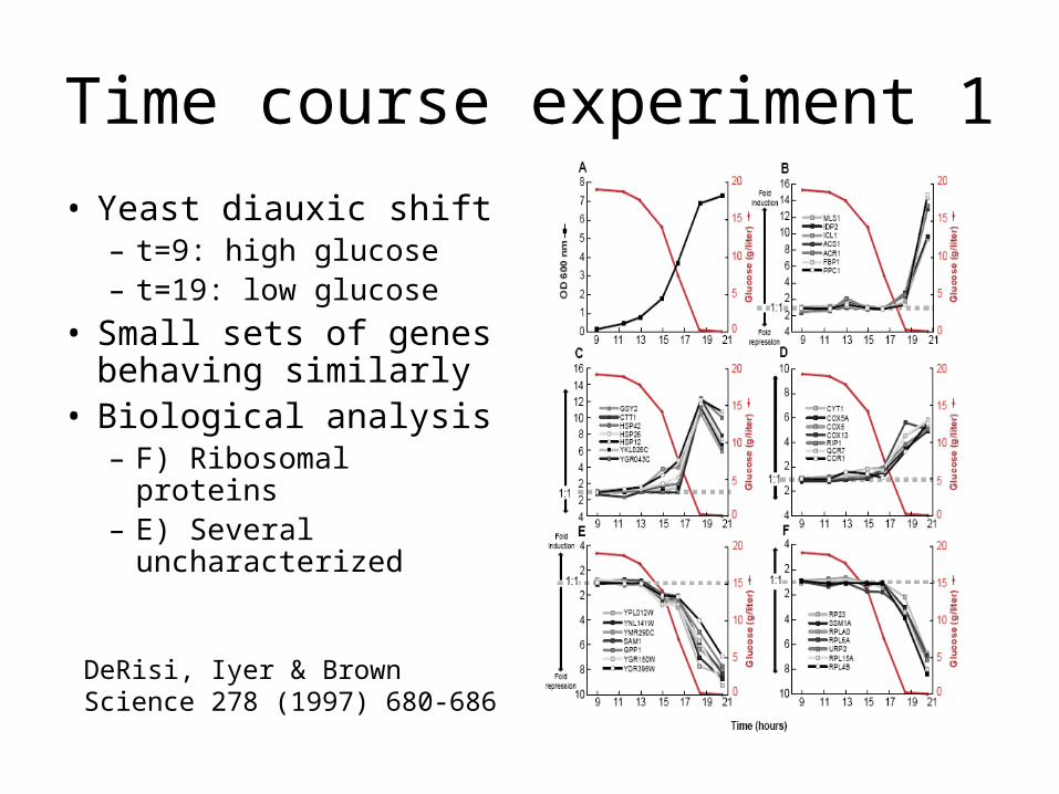
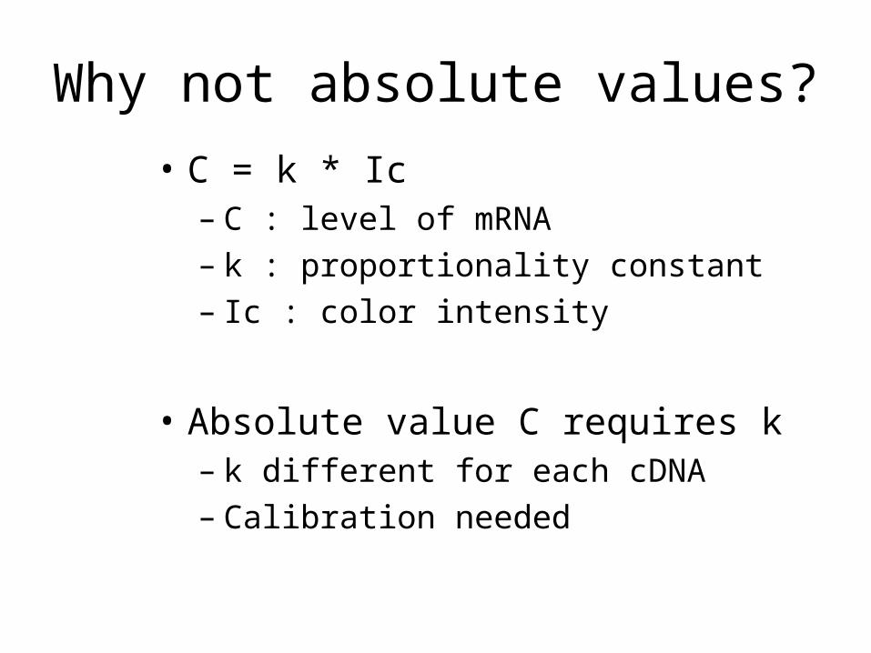
Time course experiment 1

• Yeast diauxic shift– t=9: high glucose– t=19: low glucose

• Small sets of genes behaving similarly

• Biological analysis– F) Ribosomal proteins– E) Several

uncharacterized

DeRisi, Iyer & BrownScience 278 (1997) 680-686

Time course experiment 2

• Human fibroblasts• Serum treatment• Time course; 0-24 hrs

– 12 time points• Hierarchical clustering

– Ordered by expression similarity

Iyer, et alScience 283 (1999) 83-87

Time course experiment 3

• Human fibroblasts

• Sorted according to gene function (pre-GO)

Iyer, et alScience 283 (1999) 83-87

Other approaches

• A set of “related” genes– Simplified clustering; in the set, or not

• “Related” using any criterion:– Enriched in EST data– Cluster from gene expression– Sequence similarity– Contains a specific sequence pattern– Forms a complex– …

Uncharacterized genes 1

• Goal: Identify possible classification of a previously uncharacterized gene

• “Guilt by association”– If your friend is guilty, then so are you!– If gene X and Y behave similarly in an

experiment, then both may be involved in the same biological process

Uncharacterized genes 2

• Similar gene behavior is significant if…– Statistically significant– Some genes well-characterized, as basis– Well-designed experiment

• Still, may be artifact– Spurious correlations

• Price of Cuban rum vs. Swedish pharmacist salary

– Indirectly related

Uncharacterized genes 3

• But: Other types of correlation?– Anti-correlated– Phase-shifted– Other possibilities?

• Depends on biology

GOSt• Data mining tool

– Gene Ontology– Start from a set of genes

• E.g. co-regulated in gene expression• Any other selection criterion

– Find “enriched” GO terms• Give hints for uncharacterized genes

• http://www.bioinf.ebc.ee/GOST/

• Jüri Reimand, Jaak Vilo (Tartu)

Data mining 1

• Given large amount of data…– Many different dimensions (types)– Many data points

• How to find interesting features– Correlations– Patterns– Outliers

Data mining 2

• Visualization is fundamental– Look at the data!– Look again, different angle!– Clustering, and similar, are never enough

• Many dimensions– Increasingly common in clinical setting– Novel tools

• Commercial: Spotfire, AVS,…• Open source: Mondrian,…

Data mining 3

• Patients• Parameters

– Clinical data– Biomarkers– Treatment

• Spotfire visualisation

Michael Merz, NovartisPresentation 2006Spotfire web site

Data mining 4

• Clustering is an example of data mining

• Useful in many contexts– Gene expression– Clinical data– Text analysis; text mining

• Also with smallish data sets– Example: 20 patients, 8 parameters

• Found 1 clear outlier using Spotfire visualization

Data mining 5

• NCI cancer drugs– 118 drugs– 60 human cancer

cell lines– 8000 genes

• Correlation values

• Clustering

Scherf et alNature Genetics 24 (2000) 236-244

Gene expression data

• Databases– Gene Expression Omnibus at NCBI

http://www.ncbi.nlm.nih.gov/geo/ – ArrayExpress at EBI

http://www.ebi.ac.uk/arrayexpress/ – GNF SymAtlas (Novartis Research

Foundation) http://symatlas.gnf.org/SymAtlas/

• Molecular Pharmacology of Cancer (NCI) http://discover.nci.nih.gov/nature2000/