Bioinformatics: Applications

ZOO 4903Fall 2006, MW 10:30-11:45

Sutton Hall, Room 312Jonathan Wren

Protein-Protein Interaction Networks

Lecture overview What we’ve talked about so far

Proteins & their domains Protein 3D structure

Overview Proteins do not function in a vacuum Methods of detecting protein-protein

interactions (PPI) Structure and types of networks Behavior of networks

Hopper & Mayer, 1999, Prokaryotes. Am.Sci. 87:518

Cells are crowded places!

Importance of protein-protein interactions Many cellular processes are

regulated by multiprotein complexes

Distortions of protein interactions can cause diseases

Protein function can be predicted by knowing functions of interacting partners (“guilt by association”)

Adapted from S. Fields, FEBS, 2005

A comparison of sequence (GenBank) and protein-protein interaction data (DIP database)

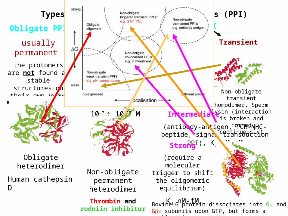
Types of protein-protein interactions (PPI)

Obligate PPI

usually permanent

the protomers are not found as stable structures on their

own in vivo

Non-obligate PPI

Obligate heterodimer

Human cathepsin D

Non-obligate transient homodimer, Sperm lysin (interaction is broken and

formed continuously)

Stable

(many enzyme-inhibitor complexes)

dissociation constant Kd=[A][B] / [AB]

10-7 ÷ 10-13 M

Transient

Weak

(electron transport

complexes)

Kd mM-M

Non-obligate permanent

heterodimer

Thrombin and rodniin inhibitor

Intermediate

(antibody-antigen, TCR-MHC-peptide, signal transduction PPI), Kd M-nM

Strong

(require a molecular trigger to shift the

oligomeric equilibrium)

Kd nM-fM

Bovine G protein dissociates into G and G subunits upon GTP, but forms a stable trimer upon GDP

Multiple interactions: Guanine-nucleotide binding protein

Adapted from Vetter & Wittinghofer, Science 2001

Multiple interactions: Guanine-nucleotide binding protein

Adapted from Vetter & Wittinghofer, Science 2001

Question: How conserved are the interactive vs non-interactive portions of this protein?

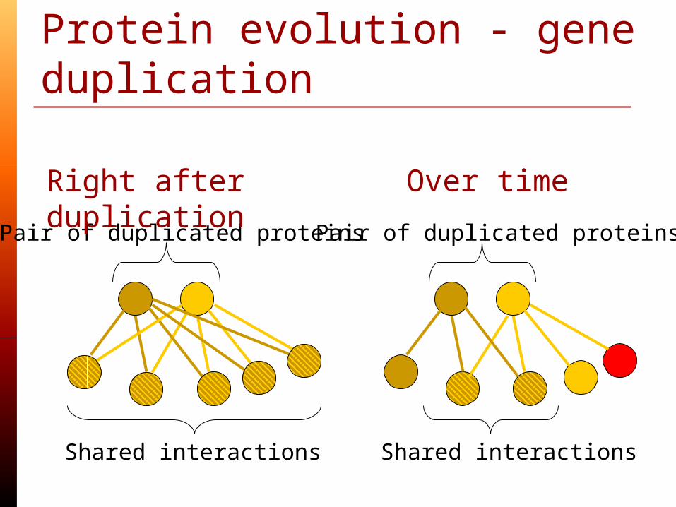
Protein evolution - gene duplication

Pair of duplicated proteins

Shared interactions

Pair of duplicated proteins

Shared interactions

Right after duplication

Over time

Methods of identifying PPIs Experimental

Protein-protein arrays Y2H assay TAP assay

Computational/Inferential Interolog analysis Co-localization, co-expression Correlated mutations Text-mining

Interologs

Homolog Common ancestors Common 3D structure Common active sites Ortholog

Derived from Speciation Paralog

Derived from Duplication

Interolog Conserved Protein-Protein

Interaction

Thus, finding one PPI may yield dividends!

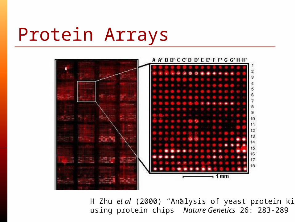
Protein Arrays

H Zhu et al (2000) “Analysis of yeast protein kinases using protein chips” Nature Genetics 26: 283-289

Reporter Gene

BaitProtein

BindingDomain

Prey Protein

ActivationDomain

Two hybrid proteins are generated with transcription factor domains

Both fusions are expressed in a yeast cell that carries a reporter gene whose expression is under the control of binding sites for the DNA-binding domain

The Two-Hybrid System

Reporter Gene

BaitProtein

BindingDomain

Prey Protein

ActivationDomain

The Two-Hybrid System Interaction of bait and prey proteins localizes the

activation domain to the reporter gene, thus activating transcription.

Since the reporter gene typically codes for a survival factor, yeast colonies will grow only when an interaction occurs.

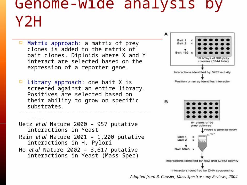
Genome-wide analysis by Y2H

Matrix approach: a matrix of prey clones is added to the matrix of bait clones. Diploids where X and Y interact are selected based on the expression of a reporter gene.

Library approach: one bait X is

screened against an entire library. Positives are selected based on their ability to grow on specific substrates.

---------------------------------------------------------

Uetz et al Nature 2000 – 957 putative interactions in Yeast

Rain et al Nature 2001 – 1,200 putative interactions in H. Pylori

Ho et al Nature 2002 – 3,617 putative interactions in Yeast (Mass Spec)

Adapted from B. Causier, Mass Spectroscopy Reviews, 2004

Advantages of Y2H In vivo technique, good approximation of

processes which occur in higher eukaryotes.

Transient interactions can be determined, can predict the affinity of an interaction.

Can be used to detect potential interactions of genes not yet observed to be translated into proteins (e.g. rarely expressed) or novel constructs (e.g. therapeutics)

Relatively fast and efficient.

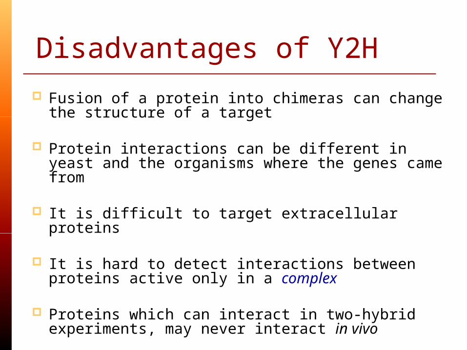
Disadvantages of Y2H

Fusion of a protein into chimeras can change the structure of a target

Protein interactions can be different in yeast and the organisms where the genes came from

It is difficult to target extracellular proteins

It is hard to detect interactions between proteins active only in a complex

Proteins which can interact in two-hybrid

experiments, may never interact in vivo

Tandem affinity purification method (TAP)

Target protein ORF is fused with the DNA sequences encoding TAP tag;

Tagged ORFs are expressed in yeast cells and form native complexes;

The complexes are purified by TAP method;

Components of each complex are found by gel electrophoresis or MS.

Tandem affinity purification method (TAP)

TAP tag consists of two IgG binding domains of Staphylococcus protein A and calmodulin binding peptide;

-------------------------------------- 7123 interactions can be clustered

into 547 complexes (Krogan et al, 2006)

O. Puig et al, Methods, 2001

Differences and similarities between Y2H and MS-TAP

TAP permits protein complexes to be isolated, but cannot detect weak/transient PPIs

Both methods generate a lot of false positives, only ~50% interactions are biologically significant

Y2H is in vivo technique

MS can detect large stable complexes and networks of interactions

Text Mining

Searching Medline or PubMed for words or word combinations

Co-occurrence of terms is the simplest metric, yet lends to a higher FP rate

NLP methods are more specific (e.g., “X binds to Y”; “X interacts with Y”; “X associates with Y” etc.) yet are difficult to detect so it has a higher FN rate

Normally requires a list of known gene names or protein names for a given organism

Pre-BIND

Used Support Vector Machine (SVM) to scan literature for PPIs

Precision, accuracy and recall of 92% for correctly classifying PPI abstracts

Estimated to capture 60% of all abstracted protein interactions for a given organism

Donaldson et al. BMC Bioinformatics 2003 4:11

From:A Protein Interaction Map of DrosophilaGiot et al. Science 302, 1727-1136 (2003)

Drosophila interaction map

Comparing large scale data of protein-protein interactions

All methods except for Y2H and synthetic lethality technique are biased toward abundant proteins.

PPI are biased toward certain cellular localizations. Evolutionarily conserved proteins have much better coverage in

Y2H than the proteins restricted to a certain organism.

Von Mering et al, Nature, 2002

Functional organization of yeast proteome: network of protein complexes

• Essential gene products are more likely to interact with essential rather than nonessential proteins

• Orthologous proteins interact with complexes enriched with orthologs

Gavin et al, Nature, 2002

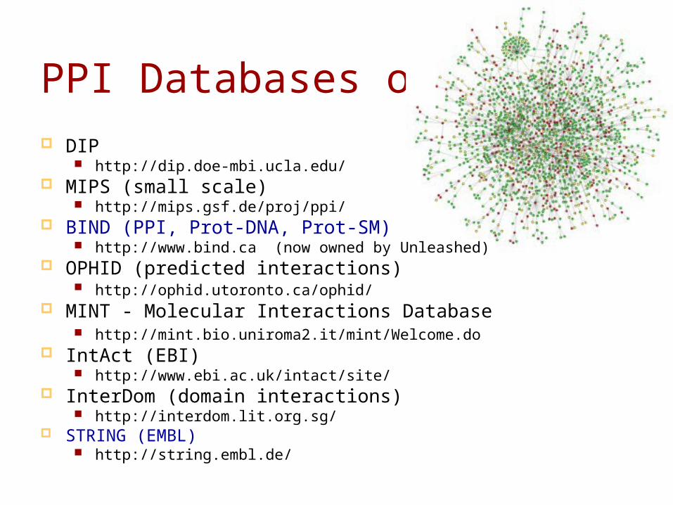
PPI Databases online DIP

http://dip.doe-mbi.ucla.edu/ MIPS (small scale)

http://mips.gsf.de/proj/ppi/ BIND (PPI, Prot-DNA, Prot-SM)

http://www.bind.ca (now owned by Unleashed) OPHID (predicted interactions)

http://ophid.utoronto.ca/ophid/ MINT - Molecular Interactions Database

http://mint.bio.uniroma2.it/mint/Welcome.do IntAct (EBI)

http://www.ebi.ac.uk/intact/site/ InterDom (domain interactions)

http://interdom.lit.org.sg/ STRING (EMBL)

http://string.embl.de/

Interaction databasesTypes Experiment (E) Structure detail (S) Predicted

Physical (P) Functional (F)

Curated (C) Homology modeling

(H) *International

Molecular Exchange (IMEx) consortium

Comparing the DBs High FP rate in high-

throughput exp. Disagreement between

benchmark sets Experimental PPI data is

sparse relative to all PPIs, so dataset overlap is small and hard to confirm with multiple sources

28

PPI network properties

Nodes & connections

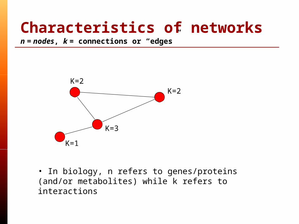
Characteristics of networksn = nodes, k = connections or “edges”

K=2K=2

K=3

K=1

• In biology, n refers to genes/proteins (and/or metabolites) while k refers to interactions

Examples of networks: Proximity-based interactions

Examples of networks: Distant interactions

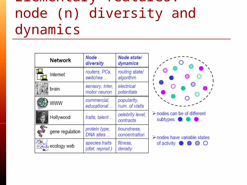
Elementary features:node (n) diversity and dynamics

Elementary features:edge (k) diversity and dynamics

Elementary features:Network Evolution

Network properties Network Structure Metrics

Average path length Degree distribution(connectivity) Clustering coefficient

Network Structure Types Regular Random Small-world Scale-free

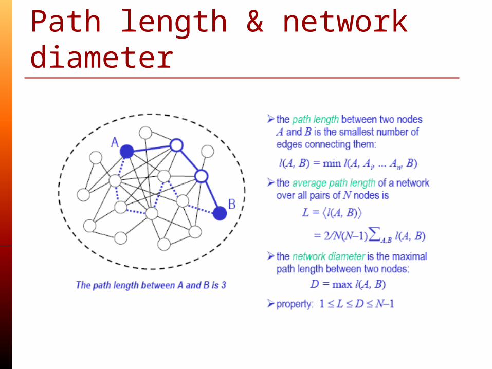
Structural metrics: Path length & network diameter

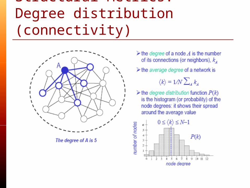
Structural Metrics:Degree distribution (connectivity)

Structural Metrics:Clustering coefficient

Network properties Network Metrics

Average path length Degree distribution(connectivity) Clustering coefficient

Network Structures Regular Random Small-world Scale-free

Regular networks – fully connected

Regular networks –Lattice

Regular networks –Lattice: ring world

Random networks

Random Networks

Small-world networks

Exponential network degree distribution

.

.

.

.

Scale-free networks

Coined by A.L. Barabasi in 1998

New nodes preferentially attach to highly connected ones

Different network models: Barabasi-Alberts.Model of preferential attachment. At each step, a new node is added to the graph. The new node is attached to one of old nodes with probability

proportional to the vertex degree.

ln(P(k))

ln(k)

kkp )(

Degree distribution – power law distribution.

Barabasi & Albert, Science, 1999

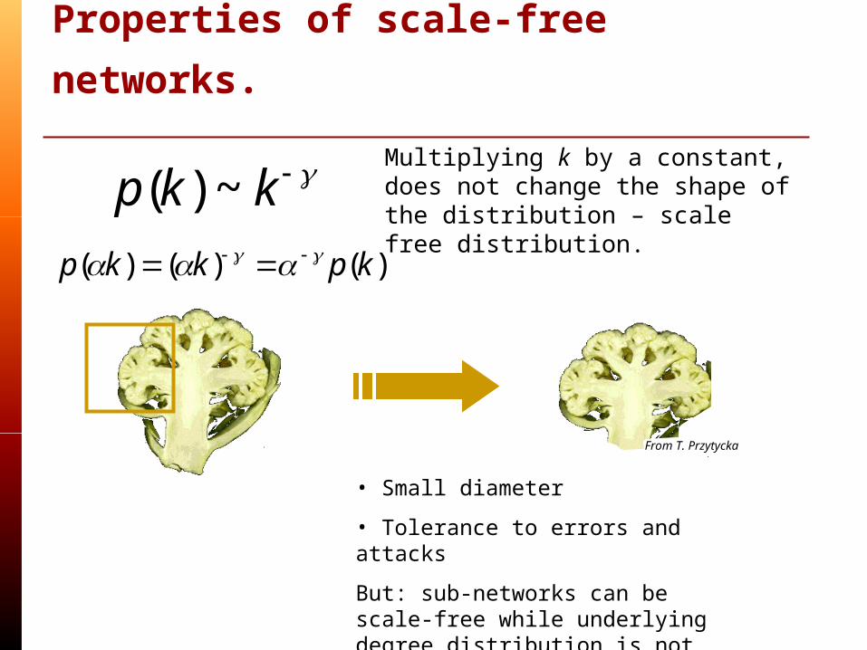
Properties of scale-free networks.

kkp ~)(

)()()( kpkkp

Multiplying k by a constant, does not change the shape of the distribution – scale free distribution.

From T. Przytycka

• Small diameter

• Tolerance to errors and attacks

But: sub-networks can be scale-free while underlying degree distribution is not.

Difference between scale-free and random graph models.

Random networks are homogeneous, most nodes have the same number of links.

Scale-free networks have a number of highly connected verteces.

Adapted from Jeong et al, Nature, 2000

.

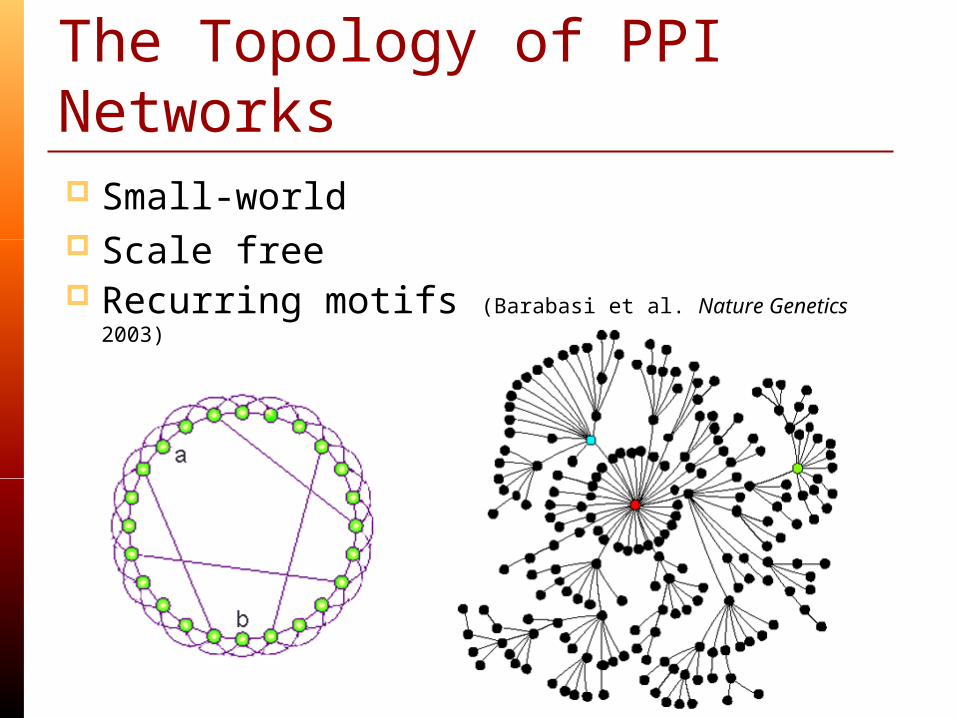
The Topology of PPI Networks Small-world Scale free Recurring motifs (Barabasi et al. Nature Genetics 2003)

Reprinted from Linked: The New Science of Networks by Albert-Laszlo Barabasi

The Internet

Category: Internet Topology Description: Internet connectivity snapshot using Skitter data and Walrus visualization

Category: Natural NetworksDescription: Yeast protein network map, inside cell

Category: Natural NetworksDescription: Portion of food web in North Atlantic Ocean

Category: Social NetworksDescription: Individuals and their professions in the network of activities during the German Revolution of 1848-1849

Category: Economic NetworksDescription: World Trade network, 1992

Metabolic Networks

• The metabolic networks of all organisms in all three domains of life (prokaryote, eukaryote, archaea) appear to be scale-free (43 examined)

• The network diameter of all 43 metabolic networks is the same, irrespective of the number of proteins involved.

• Does this seem counter-intuitive?

Implications – Attack Tolerance

Robust. For <3, removing nodes does not break network into islands.

Very resistant to random attacks, but attacks targeting key nodes are more dangerous.

Ma x

Clu

s te r

Siz

e P

ath

Leng

th

61

Order, complexity and chaos

Principles of evolution

Evolutionary puzzle The cell is constructed from unreliable

parts and is subjected to mutations, yet it behaves in a robust and reliable manner.

Can natural selection alone explain this? Or might some additional principles also come into play, such as self-organization?

Kaufmann’s hypothesis: Natural selection acts on self-organizing systems, rather than creating them. Without an innate tendency toward order, most mutations would be fatal.

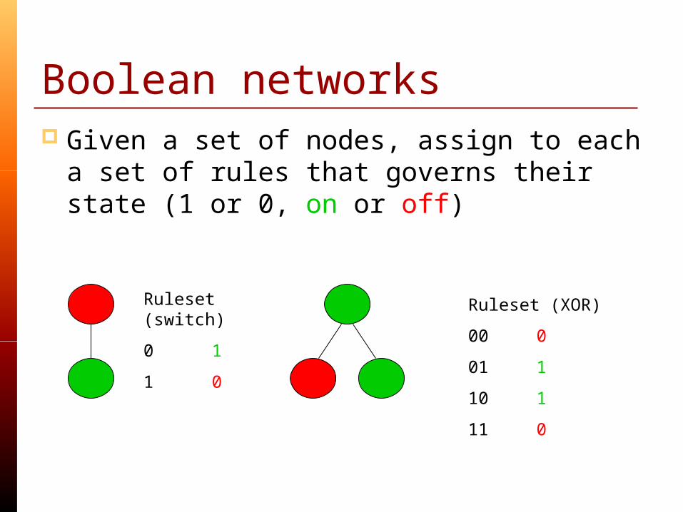
Boolean networks Given a set of nodes, assign to each a set

of rules that governs their state (1 or 0, on or off)

Ruleset (switch)

0 1

1 0

Ruleset (XOR)

00 0

01 1

10 1

11 0

Boolean networks Given a set of nodes, assign to each a set

of rules that governs their state (1 or 0, on or off)

Ruleset (switch)

0 1

1 0

Ruleset (XOR)

00 0

01 1

10 1

11 0

Boolean networks Given a set of nodes, assign to each a set

of rules that governs their state (1 or 0, on or off)

Ruleset (switch)

0 1

1 0

Ruleset (XOR)

00 0

01 1

10 1

11 0

Network behavior Given this type of setup for network

structure, what does the network behave like? Does behavior change as n increases? Does behavior change as k increases? What do sparsely connected networks behave

like? What do highly connected networks behave

like? We can answer this with a simulation…

Complexity Ordered behavior is characteristic of genomic and

metabolic networks: they quickly settle down into periodic patterns of activity that resist disturbance or cycle thru states.

Chaotic behavior is characteristic of many non-biological complex systems: sensitivity to initial conditions, long transients, and very large limit cycles (strange attractors).

BUT… Life exists and evolves in a region between order and chaos, termed “complexity” because it exhibits enough order to be stable & reproducible, but enough variation & instability to adapt to change

Summary PPI networks are one of the most active areas of

bioinformatics research interest PPI networks are constructed by empirical &

computational methods Networks have a structure that dictates their

behavior Biological networks are scale-free Essential proteins have high connectivity Life evolves on the edge between order & chaos

For next time Supplementary reading S4