Biodegradation and Transport of Crude Oil in Sand and Gravel Beaches of Arctic Alaska

Principal Investigator Dr. Silke Schiewer

Graduate Students Anna Iverson Priyam Sharma Department of Civil & Environmental Engineering University of Alaska Fairbanks FINAL REPORT July 2015 OCS Study BOEM 2015-041

Contact Information: email: CMI@alaska.edu phone: 907.474.6782 fax: 907.474.7204 Coastal Marine Institute School of Fisheries and Ocean Sciences University of Alaska Fairbanks P. O. Box 757220 Fairbanks, AK 99775-7220 This study was funded in part by the U.S. Department of the Interior, Bureau of Ocean Energy Management (BOEM) through Cooperative Agreement M14AC00020 between BOEM, Alaska Outer Continental Shelf Region, and the University of Alaska Fairbanks. This report, OCS Study BOEM 2015-041, is available through the Coastal Marine Institute, select federal depository libraries and electronically from http://www.boem.gov/Environmental-Stewardship/Environmental-Studies/Alaska-Region/Index.aspx. The views and conclusions contained in this document are those of the authors and should not be interpreted as representing the opinions or policies of the U.S. Government. Mention of trade names or commercial products does not constitute their endorsement by the U.S. Government. .

CONTENTS

LIST OF FIGURES ...........................................................................................................................v

LIST OF TABLES .............................................................................................................................vi

LIST OF ACRONYMS .....................................................................................................................vii

ABSTRACT .......................................................................................................................................ix

INTRODUCTION .............................................................................................................................1 Background ........................................................................................................................................1 Oil exploration in the Arctic .........................................................................................................1 Oil spill management in the Arctic ...............................................................................................1 Oil spill cleanup methods..............................................................................................................1 Objectives ..........................................................................................................................................2 Hypotheses .........................................................................................................................................3 Microcosm experiments ................................................................................................................3 Mini-column experiments .............................................................................................................4

LITERATURE REVIEW ..................................................................................................................4 Factors affecting biodegradation ........................................................................................................4 Role of temperature.......................................................................................................................4 Role of nutrients ............................................................................................................................5 Role of seawater salinity ...............................................................................................................6 Role of crude oil characteristics ....................................................................................................6 Role of evaporation .......................................................................................................................7 Role of sediment characteristics ...................................................................................................7 Environmental Sensitivity Index...................................................................................................8

METHODS ........................................................................................................................................8 Sediment sampling .............................................................................................................................8 Microcosm experiment ......................................................................................................................9 Analytical methods ............................................................................................................................12 Titration to determine CO2 production.........................................................................................12 Gas chromatography/flame ionization detection ..........................................................................12 Gas chromatography/mass spectroscopy ......................................................................................13 Most probable number ..................................................................................................................13 Mini-column studies ..........................................................................................................................15 Construction of mini-columns ......................................................................................................15 Experimental design......................................................................................................................15 Methodology for mini-column experiments .................................................................................16 Wave tank study .................................................................................................................................18

iii

RESULTS AND DISCUSSION ........................................................................................................18 Microcosm experiments .....................................................................................................................18 Carbon dioxide production in microcosms at 20°C ......................................................................19 Volatilization in microcosms at 20°C ...........................................................................................20 Hydrocarbons remaining in sediments in microcosms at 20°C ....................................................21 Carbon dioxide production in microcosms at 3°C ........................................................................21 Volatilization in microcosms at 3°C .............................................................................................23 Hydrocarbons remaining in sediments in microcosms at 3°C ......................................................23 Carbon dioxide production in microcosms at both temperatures .................................................26 Volatilization in microcosms at both temperatures ......................................................................27 Hydrocarbons remaining in sediments in microcosms at both temperatures ...............................27 Mass balance of crude oil in microcosms at both temperatures ...................................................28

Mini-column experiments ..................................................................................................................29 Crude oil movement in sandy gravel-sediment ............................................................................30 Carbon dioxide release in sandy gravel-sediment ........................................................................31 Effect of fertilization & temperature in sandy gravel ...................................................................33 Crude oil movement in pebble sediment ......................................................................................34 Carbon dioxide release in pebble sediment ..................................................................................36 Effect of fertilization & temperature in pebble sediment .............................................................37 Respiration ....................................................................................................................................39 Comparison of sediment types at 20 °C ........................................................................................39 Comparison of sediment types at 3°C ...........................................................................................41

CONCLUSIONS................................................................................................................................43 Microcosms ...................................................................................................................................43 Mini-columns ................................................................................................................................45

RECOMMENDATIONS ...................................................................................................................46

ACKNOWLEDGEMENTS ...............................................................................................................46

REFERENCES ..................................................................................................................................47

APPENDIX ........................................................................................................................................50

iv

LIST OF FIGURES

Figure 1. Sampling locations .......................................................................................................................... 9

Figure 2. Illustration of microcosm containing sediments with crude oil ....................................................... 10

Figure 3. MPN plate with crude oil as a carbon source .................................................................................. 14

Figure 4. Column design used in the experiment ............................................................................................ 15

Figure 5. Mini-column experimental set-up ................................................................................................... 16

Figure 6. Wave tank schematic ....................................................................................................................... 18

Figure 7. Cumulative CO2 production at 20°C ............................................................................................... 19

Figure 8. Cumulative CO2 production due to crude oil at low salinity and 20°C .......................................... 20

Figure 9. Amount of volatile compounds released per week from the crude oil at 20°C ............................... 20

Figure 10. Total petroleum hydrocarbons remaining in sediments at 20°C ................................................... 21

Figure 11. Percentage of TPH removal from sediments over 6 weeks at 20°C .............................................. 22

Figure 12. Cumulative CO2 production at 3°C ............................................................................................... 23

Figure 13. Cumulative CO2 production due to crude oil for low salinity at 3°C ............................................ 23

Figure 14. Amount of volatile compounds released per week from the crude oil at 3°C ............................... 24

Figure 15. Total petroleum hydrocarbons remaining in sediments at 3°C ..................................................... 25

Figure 16. Percentage of TPH removal from sediments over 6 weeks at 3°C ................................................ 26

Figure 17. Cumulative CO2 produced in 6 weeks at 20°C and 3°C ............................................................... 26

Figure 18. Percentage of volatile compounds released during 6 weeks at 20°C and 3°C .............................. 27

Figure 19. Percentage of TPH removal from sediments over 6 weeks at 20°C and 3°C ................................ 27

Figure 20. Mass balances of crude oil at 20°C and 3°C after 6 weeks. Graph shows fractions mineralized (CO2), volatilized (VOC) and remaining in soil (TPH) .................................................................................. 29

Figure 21. TPH concentration at different depths after 3-12 days in sandy-gravel at 20°C ........................... 31

Figure 22. TPH concentration at different depths after 3-18 days in sandy-gravel at 3°C ............................. 31

Figure 23. Cumulative CO2 released from sandy-gravel at 20°C ................................................................... 32

Figure 24. Cumulative CO2 released from sandy-gravel at 3°C ..................................................................... 32

Figure 25. Effect of temperature on TPH concentrations in samples with no fertilizer and with liquid fertilizer ........................................................................................................................................................... 33

Figure 26. Effect of temperature on release of CO2 from sandy-gravel with liquid fertilizer ....................... 34

Figure 27. TPH concentration at different depths after 3-18 days in pebble sediment at 20°C. ..................... 35

Figure 28. TPH concentration at different depths after 3-18 days in pebble sediment at 3°C ........................ 35

Figure 29. Cumulative CO2 released from pebble sediment at 20 °C ............................................................ 37

v

Figure 30. Cumulative CO2 released from pebble sediment at 3°C ............................................................... 37

Figure 31. Temperature effect on crude oil movement in pebble sediment with no fertilizer ........................ 38

Figure 32. Temperature effect on crude oil movement in pebble sediment with liquid fertilizer ................... 38

Figure 33. Temperature effect on release of CO2 from pebble sediment with fertilizer ................................ 39

Figure 34. Impact of sediment type on crude oil movement at 20°C with no fertilizer and with liquid fertilizer ........................................................................................................................................................... 40

Figure 35. Impact of sediment type on CO2 release at 20°C with liquid fertilizer ......................................... 41

Figure 36. Impact of sediment type on crude oil movement at 3°C with no fertilizer, with liquid fertilizer, and with solid fertilizer ................................................................................................................................... 42

Figure 37. Impact of sediment type on CO2 release at 3°C with fertilizer ..................................................... 43

Figure A1. MPN of crude oil degraders from 20°C experiments ................................................................... 50

Figure A2. MPN plate for the C1S2 and C2S1 samples at 20°C with crude oil as C source ......................... 51

Figure A3. MPN plate for C2S1 and C2S2 samples at 3°C with diesel as C source ..................................... 52

Figure A4. Addition of pebble sediment ......................................................................................................... 52

Figure A5. Addition of sandy-gravel sediment ............................................................................................... 53

Figure A6. Waterline on sediments ................................................................................................................. 53

Figure A7. Wave tank in action ...................................................................................................................... 54

Figure A8. Sequence of steps in wave tank experiment ................................................................................. 54

LIST OF TABLES

Table 1. Sampling location coordinates .......................................................................................................... 9

Table 2. Experimental parameters for microcosms at 20˚C and 3˚C .............................................................. 11

Table 3. Microcosm sampling schedule .......................................................................................................... 12

Table 4. Sampling schedule for replicate microcosm jars .............................................................................. 12

Table 5. Conditions in each column experiment ............................................................................................. 16

Table 6. Column flush cycle ........................................................................................................................... 17

Table A1. MPN values of number of microbes per gram of soil at 20°C ....................................................... 50

vi

LIST OF ACRONYMS

API American Petroleum Institute

BOEM Bureau of Ocean Energy Management

C0 no crude oil added

C1 1 mL crude oil added

C2 5 mL crude oil added

ESI Environmental Sensitivity Index

GC/FID Gas Chromatography with Flame Ionization Detector

GC/MS Gas Chromatography with Mass Spectrometry

MPN Most Probable Number

PAH Polycyclic Aromatic Hydrocarbons

PVC Polyvinylchloride

S1 Low salinity of 30 g/L

S2 High salinity of 35 g/L

UAF University of Alaska Fairbanks

VOC Volatile Organic Compounds

WERC Water and Environmental Research Center

TPH Total Petroleum Hydrocarbons

vii

ABSTRACT

Offshore oil production along Alaska’s arctic coast is expected to increase in coming years. While this will create large economic benefits for the state, crude oil spills may occur. Oil spills reaching the shoreline could create adverse ecological effects, so it is important to understand methods, such as bioremediation, that might expedite oil removal. Mass transfer processes play an important role in determining the fate of crude oil along shorelines. Biodegradation and mass transfer processes are strongly dependent on temperature and sediment material. It is, therefore, necessary to study how the beach matrix, temperature, and nutrient addition affect the fate of hydrocarbons.

The effect of environmental conditions on the rate of crude oil removal was studied in the laboratory, simulating oil spills at arctic seashores. Laboratory microcosms were set up containing beach sediments collected from Barrow, spiked with North Slope Crude. The microcosms were spiked with a standard concentration of nutrients and incubated at varying temperatures (3°C vs. 20°C), salinities (30 vs. 35 g/L), and crude oil concentrations (1 vs. 5 mL/kg). Respiration rates (breakdown of hydrocarbons to CO2), hydrocarbons remaining in the sediment (GC/FID), and hydrocarbons volatilized and sorbed to activated carbon (GC/MS) were measured. Mini-column experiments to simulate the transport of oil through the sediment profile were conducted for two different sediment types (sandy-gravel versus pebble) obtained from Barrow and two different temperatures (20° and 3° Celsius).

In all microcosms, higher respiration rates by naturally occurring microorganisms were observed at 20ºC compared to 3°C. Surprisingly, the release of volatile organic compounds (VOC) was similar at both temperatures, for different crude oil concentration and salinities. Regardless of temperature, increased salinity had a positive impact on the rate of crude oil removal. At higher crude oil dosages, a larger amount of volatiles was released; however, CO2 production did not significantly increase with the contaminant concentration. A mass balance was established that showed that only a small fraction of the crude oil was mineralized, approximately 40% was volatilized and most TPH remained in the sediment.

Mini-column data showed that the amount of crude oil pooling and its location was dependent on sediment structure and fertilizer addition. In sandy gravel sediment, TPH pooled in the middle of the column, six inches below the surface. In pebble sediment, the highest TPH concentrations initially occurred at the top and then at the bottom of the column. Overall, less TPH remained in pebble sediment compared to sandy gravel. Apparently hydrocarbons had been washed out more easily from pebble sediment. Both sediments had higher CO2 production at higher temperatures, with the highest respiration found in sandy-gravel, i.e., more biodegradation occurs in sandy-gravel sediment. While CO2 releases were slightly higher in sediments with the addition of fertilizer; overall the application of fertilizer did not have a significant impact on CO2 release.

The results of this study will assist decision-makers in choosing effective spill response strategies for future crude oil spills in Arctic shorelines.

ix

1

INTRODUCTION

Background

Oil exploration in the Arctic

The expected increase in offshore oil production in Alaska, combined with the potential opening

of the Northwest Passage in the coming years, could lead to an increase in barge and tanker

traffic through the Arctic. Increased exploratory drilling in the Chukchi and Beaufort Seas can

increase the risk of oil spills in Alaska’s arctic marine waters. While oil production provides

economic benefits to local communities and the state of Alaska, related activities have the

potential to adversely affect ecosystems, as well as the livelihood of local residents, especially

when it is based on subsistence fishing. The commercial benefits of increased oil revenues must

be weighed against the potential environmental costs of oil spills. Due to its remoteness and

harsh weather, Alaska’s Arctic coast has limited infrastructure such as ports, roads and airports

(CRRC 2010), which makes oil spill response more difficult. Therefore, it becomes important to

investigate which oil spill response strategies might be most effective in such conditions.

Oil spill management in the Arctic

Overall management of oil spills is increasing in complexity and magnitude worldwide

(Othumpangat and Castranova 2014). The most effective response strategy for a specific spill

depends on a number of factors, such as type of oil (viscosity, composition), geology, amount of

turbulent energy, temperature, sea and air currents, sensitivity of biological communities and

water salinity (EPA 2014, Owens and Lee 2003). Further, rapid removal of spilled oil is

important to reduce the harmful effects of oil spills on sensitive habitats (EPA 2014). For any oil

response, the oil company and other oil spill response organizations should have a generalized

protocol follow (Sydnes and Sydnes 2013).

Clean-up of oil spills in Arctic waters poses significant challenges because of harsh conditions.

Inadequate infrastructure and poor weather can delay the arrival of vessels, equipment, and other

supplies, and the presence of ice can confound response efforts by interfering with mechanical

oil removal (PEW Charitable Trust 2013). It is critical to identify technologies and recovery

techniques specifically tailored to oil spill clean-up in Arctic waters.

Oil spill cleanup methods

There are mechanical, chemical and biological methods for oil spill response. Mechanical

methods include the use of skimmers, sorbent barriers, and inflatable booms, the latter most

frequently used to concentrate oil on the water surface for easier recovery. Skimmers draw the

oil from the water surface, and sorbent materials absorb the oil (EPA 2014). Chemical methods

include the use of dispersants that break down the oil into tiny droplets, creating more surface

area for degrading microbes (EPA 2014). Herders are chemicals that thicken oil spills so they

can undergo in situ burning. Biological methods rely on microbial degradation for removing the

spilled oil. Biodegradation use as an oil removal process is well documented in the literature

2

(Brakstad and Bonaunet 2006) and can be an affordable and environmentally beneficial approach

for removing hydrocarbons (Prince et al. 2003).

Biodegradation is the breakdown of complex compounds into simple molecules by microbes.

Bioremediation is a specific case of biodegradation, where the latter is used as an engineered

method to degrade undesired complex compounds. To accelerate biodegradation, bioremediation

strategies may include the addition of nutrients or electron acceptors to accelerate the growth and

metabolic rate of micro-organisms (biostimulation) and/or the addition of oil-degrading microbes

at the contaminated region (bioaugmentation).

Bioremediation can be a cost-effective and safe technique for cleaning up crude oil contaminated

sediments, even in Arctic and subarctic environments. A combination of mechanical removal and

bioremediation, enhanced by nutrient addition, has shown potential in clean-up efforts in the

past; for example, after the Exxon Valdez oil spill (Wrabel and Peckol 2000). In situ

bioremediation offers a promising alternative in remote locations and other areas where

mechanical removal is not feasible. However, previous studies have also shown that

bioremediation was not effective for heavy crude oil or in low-temperature environments, so

further research is necessary to evaluate conditions under which bioremediation of crude oil can

be effective in cold climates. Heiser (1999) demonstrated that, even at low temperatures, oil spill

bioremediation can be successful if there is a nutrient supply. Several researchers have concluded

that nutrient supply and adjustment of pH, oxygen, and soil moisture levels can increase the oil

biodegradation rates in Alaskan soils (Rice 2007, Heiser 1999, Horel and Schiewer 2009).

Limited research has been conducted on crude oil degradation at low temperatures in soil and on

the effect of salinity (Minai-Tehrani et al. 2009).

Arctic shorelines have not been exposed to a major oil spill, so little is known about

biodegradation of crude oil in that environment. Therefore, it is essential to study the rate of

crude oil biodegradation in arctic seashore sediments. However, sometimes results of small-scale

laboratory studies cannot directly be scaled up due to heterogeneity and concentration gradients

in larger settings (Horel and Schiewer 2015).

Objectives

The objective of this study was to investigate the combined effects of varying temperatures,

crude oil concentrations and salinities on the fate of crude oil biodegradation in laboratory

experiments simulating environmental conditions along Alaska’s arctic shore. This project

focused on evaluating the potential for crude oil biodegradation in an oil spill response along

Arctic shorelines and providing a better understanding of how crude oil interacts with the

shoreline sediment. Mass transfer processes play an important role in determining the fate of

crude oil along shorelines, and the diffusion and dispersion of oil, and its viscous properties, are

strongly temperature dependent. Penetration of oil also depends on the sediment characteristics

(Yang et al. 2009). Additionally, nutrients added to stimulate bioremediation may be washed out

by waves and tides. Therefore, it is necessary to study how factors such as the beach matrix and

temperature affect hydrocarbon and nutrient distribution.

3

Biodegradation was studied in Barrow beach sediments in laboratory microcosms as a proxy for

an actual oil spill bioremediation on the Arctic shoreline. Typical sandy-gravel beach sediments

obtained from Barrow were spiked with crude oil as the contaminant, amended with nutrients,

and incubated to determine the extent to which crude oil was degraded, volatilized or remained

in the sediments. Microcosm experiments were designed to examine the role of varying

temperature, crude oil concentration and salinities on the fate of crude oil and the degradation

rate.

In a laboratory setting, mini-columns were used to study mass transfer, simulating shoreline

conditions of the Chukchi and Beaufort Seas. The effectiveness of fertilizer addition (both solid

and liquid) was examined to determine if nutrient addition had a significant impact on CO2

production. Studies were done at two temperatures (3°C, as typical for the arctic summer, and

20°C, as typical for temperate regions), to determine if temperature has a significant effect on oil

movement and degradation. Crude oil fate was determined by tracking its movement through the

sediment profile (top, middle, and bottom) for two different sediment types to determine whether

petroleum hydrocarbons were washed out, converted to CO2 or volatilized.

Identifying where oil might pool and estimating the depth to which it might penetrate shoreline

sediments are important considerations in research on microbial degradation in the Arctic.

Furthermore, the ability to predict how an environment will react to an oil spill under specific

conditions will help inform response planning and assist decision-makers in choosing effective

spill response strategies should crude oil spills occur on Arctic shorelines.

Hypotheses

Microcosm experiments

1. Crude oil is degraded by indigenous microbes present in the Barrow sediments (i.e.,

biostimulation or inoculation with microbes is not required).

2. Mineralization of crude oil increases with increasing contaminant concentration in

absolute terms, but relative mineralization percentages will be lower for higher crude oil

concentrations.

3. Increasing crude oil concentrations lead to higher volatilization in absolute terms.

4. For higher crude oil concentrations, higher quantities of crude oil will remain in the

sediment.

5. Biodegradation is faster at higher temperatures, but even at low temperatures measurable

degradation (CO2 production) will take place over the course of several months.

6. Overall hydrocarbon removal from the soil will be greater at higher temperatures.

7. Volatilization is greater at higher temperatures.

8. Higher salinity will have a positive impact on hydrocarbon degradation rates (CO2

production).

4

Mini-column experiments

9. Remaining crude oil concentrations will be lower in pebble versus sandy-gravel

sediment.

10. Oil pooling should be visible in sandy-gravel, but not pebble sediments.

11. Lower temperatures should inhibit crude oil movement, causing higher TPH

concentrations, especially in the upper layers.

12. Higher temperatures will allow for higher CO2 production.

13. The addition of fertilizer should have a positive influence on CO2 production.

14. Solid fertilizer will increase CO2 production more than liquid fertilizer.

LITERATURE REVIEW

Factors affecting biodegradation

The rate of hydrocarbon biodegradation depends on many different factors such as nutrient

availability, microbial growth, oxygen, water content, sediment type, temperature, hydrocarbon

type, pH-value and bioavailability of contaminants (Margesin 2000). For any oil spill, all

environmental factors influence the degradation rate cumulatively. Bioremediation accelerates

the natural attenuation by optimizing the limiting environmental conditions present at a spill site

(Margesin 2000). Some of the factors particularly relevant for the present research will be

discussed in the following subsections.

Role of temperature

Temperature plays an important role in the process of biodegradation and bioremediation.

Different organisms have different optimal temperatures, depending on the environment in which

they typically occur. However, even organisms found in areas with cold climates, such as

Alaska, often show higher metabolism at room temperature than at lower temperatures. This

suggests that bioremediation is less effective at lower temperatures. Biodegradation typically

follows the Arrhenius relationship, where metabolic activity decreases with a decrease in

temperature (Heiser 1999, Yang et al. 2009). The Arrhenius relationship can also be applied to

microbial community systems, where microbial growth increases with an increase in

temperature. A study conducted by Yang et al. (2009) showed that heavy fuel biodegradation in

the North Sea was four times faster at 18ºC than at 4ºC. However, while microbial activity at low

temperatures slows down, it does not stop (Yang et al. 2009, Aislabie et al. 2006). Laboratory

experiments have shown that, though the microbial activity does not cease in a cold environment,

the rate of mineralization is still higher in warmer environments (Aislabie et al. 2006, Horel and

Schiewer 2009, Schiewer and Niemeyer 2006). Even at low temperature, there are hydrocarbon-

degrading microorganisms that occur and can survive solely on hydrocarbon products (Rike et al.

2003, Heiser 1999, Yang et al. 2009).

5

Crude oil is a complex mixture of different hydrocarbons, and its properties depend on the

surrounding temperature (Heiser 1999, Yang et al. 2009). Temperature is a critical parameter for

bioremediation as it affects the rates of hydrocarbon degradation, microbial growth and mass

transfer of substrate in cold soils (Yang et al. 2009). Additionally, the rates of volatilization are

significantly reduced as temperatures decrease (Paudyn et al. 2008).

Role of nutrients

Microbial growth would not be possible without suitable nutrients present in the system. For

growth to occur, microbes require a source of carbon (main substrate, e.g. hydrocarbon), sources

of nitrogen and phosphorus (nutrients), and electron donors/acceptors (Yang et al. 2009). In

aerobic respiration, heterotrophic microorganisms use oxygen as a terminal electron acceptor

(Rike et al. 2003). Nitrogen and phosphorous are often limiting nutrients in Arctic soils;

therefore, nutrient supplementation enhances the degradation of hydrocarbons. The addition of a

commercial fertilizer such as 20:20:20 has been demonstrated to increase the mineralization of

the majority of crude oil alkanes in Arctic soils (Aislabie et al. 2006). Amending sandy-gravel

soil (from Barrow, AK) with 50-100 mg N/kg increased hydrocarbon degradation, whereas 200

mg N/kg inhibited the degradation activity (Aislabie et al. 2006). This inhibition of soil microbial

activity could be due to nitrite toxicity (Yang et al. 2009). Redfield stoichiometry states that the

desired ratio of C, N, P and K is 100:15:1:1; therefore, it is important to supply nutrients in the

form of N and P as they often become limiting when the contaminant functions as a carbon

source (Yang et al. 2009).

The addition of nutrients to oiled sites facilitates faster microbial growth and hydrocarbon

degradation. A field study by Margesin (2000) was conducted on oil-contaminated soil at an

alpine skiing resort. The contamination had resulted from motor vehicles oil leakage and storage

tank rupture. Results showed that fertilization led to a 42% reduction in hydrocarbon

contamination, whereas natural attenuation led to a reduction of only 14% (Margesin 2000).

Similar studies at low temperatures have demonstrated a positive relationship between

degradation of oil and nutrient supply. For example, addition of fertilizer in a cold alpine soil

contaminated with diesel fuel showed 43% decontamination in 30 days (Heiser 1999).

The addition of nutrients can have a significant effect on the bioremediation of oil. Various

studies have investigated the combination of nutrients that would result in the maximum

microbial productivity. Braddock et al. (1997) found that phosphorus and nitrogen have the

greatest effect on petroleum biodegradation by microbial communities. Mohn and Stewart (2000)

found that adding phosphorous and nitrogen increased microbial activity in mineralizing

petroleum products. However, the biodegradation rate was not increased for hydrocarbons with

higher molecular weights.

Braddock et al. (1997) showed that different rates of nutrient addition to soil samples affect

microbial activity. They found that nitrogen was the most important nutrient to stimulate

microbial activity; however, nutrient addition over the 400 mg N/kg soil threshold caused

inhibition. This inhibition was assumed to be caused by reduced water availability due to

6

osmotic effects. Furthermore, the soil may have contained less moisture due to the lower

precipitation rates and higher permafrost level at the study sites. Reduced productivity may have

followed a decrease in carbon in the soil and a change in salinity.

Role of seawater salinity

The Beaufort Sea, Chukchi Sea, and the North Aleutian Basin have water temperatures and

salinity levels ranging from 5-10°C and 10-24 ‰ in the summer (CRRC 2010).

The interaction of oil and minerals (present either in the sediments, soil or rocks) is an important

factor in the clean-up of an oil spill. Recent studies have confirmed that saline seawater enhances

the formation of oil-mineral aggregates (OMA), which help in the degradation of oil and increase

biodegradation at higher salinities. Owens and Lee (2003) found that some OMA formation still

occurs under low saline conditions.

Salinity is a major factor that affects microbial activity in the marine environment (Thavasi et al.

2007). Thavasi et al. (2007) found that increased levels of salinity (33-282 g/L) decreased

hydrocarbon degradation. A study was conducted by Diaz et al. (2002) where a bacterial

consortium was immobilized on polypropylene fibers to degrade the oil in saline water. The

immobilized cells showed higher hydrocarbon degradation rates than non-immobilized cells

(Diaz et al. 2002). This is a new approach to bioaugmentation, in this case, immobilizing

microbes to increase the efficiency of degradation. High salinity can make the conventional

bioremediation of oil difficult in crude oil contaminated water (Diaz et al. 2002).

Minai-Tehrani et al. (2009) observed a positive correlation between salinity and the rate of

phenanthrene mineralization; 10g/L and 30 g/L NaCl facilitated degradation of PAHs in soil,

whereas 50g/L NaCl inhibited the microbial activity. Thavasi et al. (2007) found the strain of the

common Gram-negative bacterium Pseudomonas aeruginosa exhibited maximum

biodegradation activity and growth at 35 g/L salinity.

Most of the above experimental studies used NaCl to prepare saline water. However, one should

note actual seawater contains other constituents in addition to NaCl. Results from different

experimental studies discussed above concur that salinity does have a significant effect on oil

biodegradation; however, results differ as to what salinity level leads to the highest degradation

rates.

Role of crude oil characteristics

Crude oil is a complex mixture of hydrocarbon compounds including alkanes, cycloalkanes and

aromatic hydrocarbons (Yang et al. 2009, API 2011). The American Petroleum Institute (API)

submitted a report to the Environmental Protection Agency (EPA) in 2011 that divided crude oil

into three categories: light, medium and heavy. Crude oil is classified by its density, common

measured as API gravity. The API gravity calculation is API=141.5/specific gravity - 131.5.

Light crude has an API gravity ≥33°, heavy crude has an API gravity ≤28°, and medium crude

has values between these grades.

7

The rate of crude oil biodegradation depends on the composition of hydrocarbon compounds

present in the crude. Polycyclic aromatic hydrocarbons (PAHs) take longer than aliphatic

compounds to degrade at cold temperatures (Yang et al. 2009). In decreasing order, the

biodegradability of compounds is n-alkanes, branched-chained alkanes, branch alkenes, n-alkyl

aromatics, monoaromatics, cyclic alkanes and PAHs (Yang et al. 2009).

The crude oil concentration plays an important role in the act of degradation. Thavasi et al.

(2007) conducted a biodegradation study with substrate (crude oil) concentration varying from

0.1% - 4.5% in water. Maximum degradation activity occurred at a substrate concentration of 2%

in water samples. This experiment revealed the significance of oil concentration on its

biodegradation.

Residual crude oil is no longer degradable and contains mainly PAH and asphaltenes. A study by

Fernandez-Alvarez et al. (2006) at Sorrizo beach, which was affected by the Prestige oil spill,

monitored the rate of biodegradation of weathered fuel oil that remained after initial

volatilization and some microbial degradation. Neither biostimulation nor bioaugmentation

increased degradation of the residual fuel oil; however, the introduction of biodiesel increased

the degradation of the weathered oil (Fernandez-Alvarez et al. 2006).

The role of evaporation

Weathering of oil in the water column includes surface evaporation, droplet formation,

biodegradation and other environmental processes (Wrabel and Peckol 2000, Brakstad and

Bonaunet 2006). Wrabel and Peckol (2000) found that natural attenuation proceeded mainly by

evaporation, with little microbial degradation, when there was low nutrient availability at an oil-

spill site; 25-30% more n-alkanes were lost with the addition of nutrients (N and P). Low

temperature usually results in reduced evaporation of volatiles and a delayed start of

biodegradation (Heiser 1999, Yang et al. 2009, Aislabie et al. 2006, Margesin 2000). The

volatilization of short-chain alkanes is higher at higher temperatures.

The role of sediment characteristics

Shoreline particle size and distribution of the sediment can have a large impact on the movement

of oil. Higher porosity sediments contain a larger amount of voids allowing fluids to travel more

freely through the sediment. Sand sediment presents a much greater resistance to fluid flow

through porous media because sand grains can be more neatly packed resulting in much smaller

pore sizes. The ability for oil to be retained in soil is inversely related to its ability to penetrate

the sediment (Harper 1978). Additionally, the sediment particle size can influence how many

microbes are present in the soil. If sediment has large grain size (such as pebbles), there is less

surface area for organic matter and moisture to be retained, making it a harsh environment for

microbes to survive.

Sediment characteristics are also an important factor in determining the fate of crude oil in

sediments. Every beach is different in terms of climate, grain size distribution and biological and

chemical characteristics. The components of the beach sediments govern the possible effects of

8

oil on the shoreline (EPA 2014). The eastern Beaufort Sea coastal sediments contain a large

amount of organic carbon due to river inputs and coastal erosion of peat. However, the fate of

this organic matter in the sediments is still unknown (CRRC 2010). During storms, these

sediments can be redistributed. In the Barrow area, separate zones of mostly pebbles alternate

with those that are mostly sand. If an oil spill occurs on such a beach, oil could penetrate up to 50

cm depth (pooling there) and storms can erode some surface-spilled oil (NOAA 2002).

Oil movement deeper into the sand renders degradation difficult due to limited availability of

oxygen (EPA 2014). Tilling has been used as an oil spill response method on oiled beaches.

Tilling allows escaped oil to materialize on the surface where microbes can readily degrade the

oil because of oxygen availability. Tilling accelerates physical, chemical and biological

processes that would be absent or slower under natural conditions (Owens and Lee 2003). An

EPA study (2014) was conducted on a soil plot where IF-30 intermediate fuel was used as a

contaminant, and the role of tilling and fertilizer addition was monitored. The tilled sediment

with fertilizer showed the maximum oil degradation compared to untilled and unfertilized

sediment.

Environmental Sensitivity Index

Since coastal environments respond differently to oil spills, the National Oceanic and

Atmospheric Administration (NOAA) developed an Environmental Sensitivity Index (ESI) that

classifies susceptibility to oil spills on the basis of three factors: shoreline classification,

biological resources and human use resources (NOAA 2002). The ESI shoreline classifications

range from 1 (high levels of physical energy and low biological activity) to 10 (sheltered

shorelines, high biological activity). By looking at substrate type, grain size, wave action, tidal

currents and river currents, a prediction of behavior and persistence of oil in intertidal habitat can

be made. If a spill were to occur, responders could then look up the affected shoreline’s

characteristics and determine its ESI number; which gives the responder a general idea of how

oil will react in the environment, and what potential problems could arise. ESI maps have been a

vital part of oil spill response and planning since 1979.

The North Slope contains shorelines that fall under ESI 1, 4 and 5. This research will focus on

sediments typical of ESI 4 and 5 areas, coastlines predominantly composed of sand and gravel

sediment (NOAA 2002). Much of the Chukchi Sea and Beaufort Sea region falls under the ESI

5B category, which is characterized by mixed sand with at least 20% gravel, an intermediate

slope of 8-15 degrees, and low fauna and epifauna populations (NOAA 2002).

METHODS

Sediment sampling

Sediment samples were collected from July 22 - 25, 2013 at a four beach locations near the city

of Barrow, the local hub of Alaska’s northern coast at the intersection of the Beaufort and

Chukchi Seas. Four 10-gallon buckets were filled from the top 60 cm of beach sediment (roughly

30 kg per bucket). Samples were collected at four different locations (Figure 1, Table 1). Two

9

buckets were collected along the Beaufort Sea/Elson Lagoon, where the sediment had a more

sandy-gravel composition (4-ESI). Two buckets were collected along the Chukchi Sea; these

sediments were primarily composed of pebble material (5-ESI). The samples were transported

back to the laboratory and kept at 4°C. Water samples were collected from the sea adjacent to

each sampling site and returned to the laboratory where salinity (30 g/L) was determined by

salinity meter.

A sandy gravel sample with some pebbles collected at 71°21'39.80"N, 156°21'47.90"W was used

for the microcosms. One bucket of each ESI type was used to determine the fate of crude oil for

a variety of conditions both in mini-column and wave tank studies. The two sediment types were

classified as sandy-gravel and pebble, respectively.

Figure 1. Sampling locations.

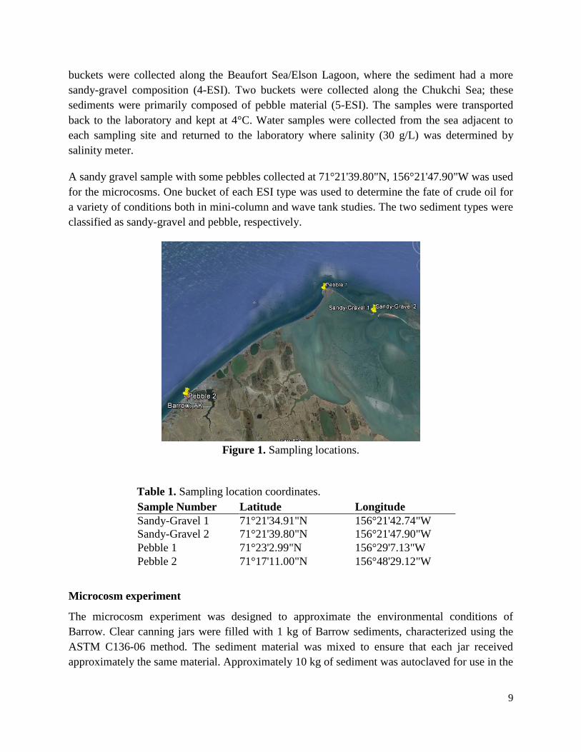
Table 1. Sampling location coordinates.

Sample Number Latitude Longitude

Sandy-Gravel 1 71°21'34.91"N 156°21'42.74"W

Sandy-Gravel 2 71°21'39.80"N 156°21'47.90"W

Pebble 1 71°23'2.99"N 156°29'7.13"W

Pebble 2 71°17'11.00"N 156°48'29.12"W

Microcosm experiment

The microcosm experiment was designed to approximate the environmental conditions of

Barrow. Clear canning jars were filled with 1 kg of Barrow sediments, characterized using the

ASTM C136-06 method. The sediment material was mixed to ensure that each jar received

approximately the same material. Approximately 10 kg of sediment was autoclaved for use in the

10

sterile control microcosms. To evaluate biodegradation by the naturally present microorganisms,

sediment used in the experimental microcosms was not sterilized. No inoculation was performed.

Figure 2 below shows the experimental setup for this study. In each microcosm, a “tea bag” (one

side open) made from mosquito netting, with a size of 10x8 cm, was filled with 5 g of coconut

shell activated carbon and suspended with a string in the jar’s headspace to trap the volatile

compounds released from the crude oil. Each jar had a metal loop stand, prepared from a 12-inch

steel wire inserted into the sediment, to suspend a beaker filled with 20 mL of 1 N NaOH

solution in the headspace. Each jar received 10 mL of nutrient solution prepared from fertilizer

with an N:P:K ratio of 20:20:20; the nitrogen fraction consisted of 20% ammonia, 30% nitrate,

and 50% urea nitrogen. Each microcosm received a total nitrogen concentration of 300 mg/kg

sediment.

Figure 2. Illustration of microcosm containing sediments with crude oil.

Quadruple microcosms were set up to represent seven different conditions, three as controls and

four experimental, with varying crude oil concentrations and salinities as specified in Table 2.

Twenty-eight jars were prepared for each temperature regime (20°C and 3°C). Microcosm jars

were tightly sealed and placed inside a fume hood for 6 weeks for the 20˚C series and kept in a

refrigerator for 9 weeks for the 3°C series.

Table 2. Experimental parameters for microcosms at 20˚C and 3˚C.

Type Setup ID Crude Oil

(mL/kg)

Salinity (g/L) Sterilized No. replicate

Jars

contr

ol C0S1 0 30 -- 4

C0S1 0 30 yes 4

C1S1 1 30 yes 4

Exper

imen

tal C1S1 1 30 -- 4

C1S2 1 35 -- 4

C2S1 5 30 -- 4

C2S2 5 35 -- 4

11

Experiments were performed at two different salinities. Sediments brought from Barrow had

been naturally saturated with ocean water of a salinity of 30 g/L. This material was used for S1

(low salinity of 30 g/L) experiments. For the high salinity (S2) experiments, sediment was

flushed with artificial seawater (35 g/L salinity prepared using Instant Ocean Aquarium Salt)

before filling the jars.

Either 1 or 5 mL of crude oil was pipetted onto the sediment surface. The specific gravity of

crude oil was measured at 0.87 at 20°C and 3°C. Therefore, the initial concentration of added

crude oil was 870 mg/kg for 1 mL of crude oil added and 4350 mg/kg for 5 mL of crude oil.

After addition of crude oil and fertilizer, the sediment was mixed vigorously with a spoon as a

proxy for sediment tilling.

The experiment was designed to establish a mass balance for the initially present crude oil

including volatilization of short chained hydrocarbons, crude oil remaining in the sediment, and

crude oil mineralized (converted to carbon dioxide). The following parameters were used to

evaluate the results:

1. CO2 produced and captured in NaOH solution was quantified by titration with HCl.

2. Volatiles released from the crude oil and captured by activated carbon were assessed via

gas chromatography/mass spectrophotometry (GC/MS).

3. Crude oil remaining in the sediments was determined by gas chromatography/flame

ionization detector (GC/FID).

4. Number of microbes present in the sediments was calculated by using the most probable

number (MPN) method.

The sampling frequencies for the above parameters are shown in Table 3. Additionally, each

temperature series had four replicate microcosm jars (A-D) for each environmental condition,

and these were sacrificed for sampling every two or three weeks (Table 4).

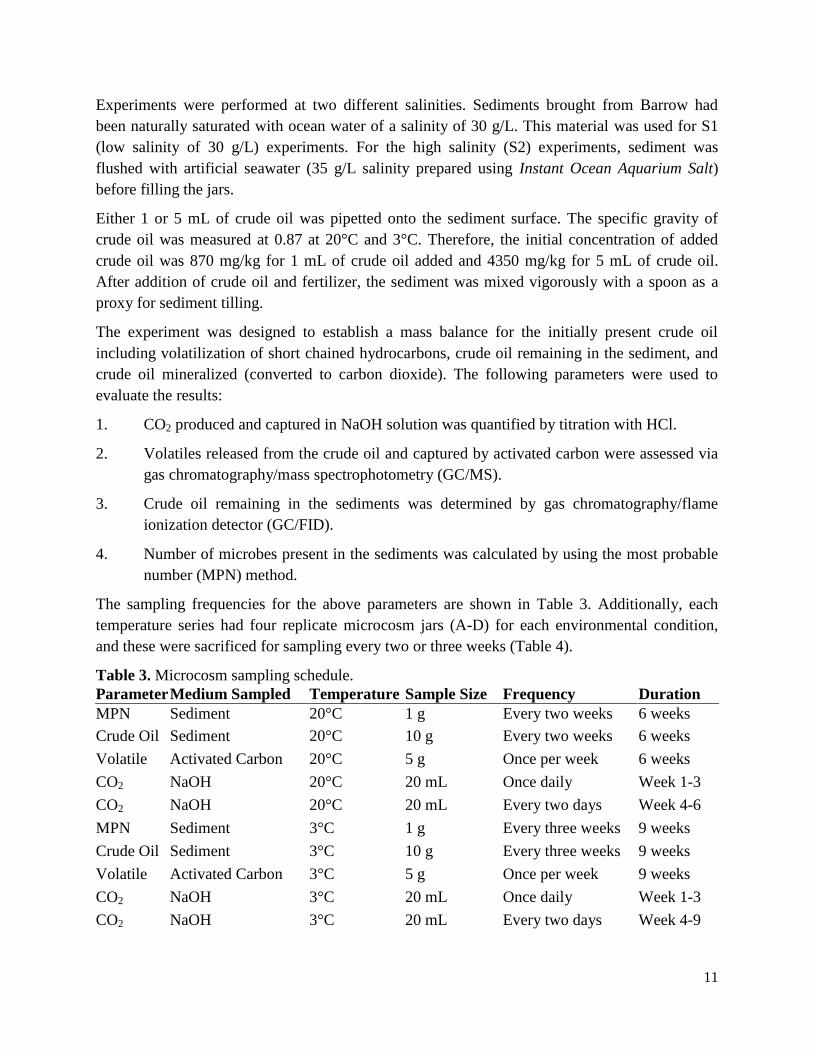
Table 3. Microcosm sampling schedule.

Parameter Medium Sampled Temperature Sample Size Frequency Duration

MPN Sediment 20°C 1 g Every two weeks 6 weeks

Crude Oil Sediment 20°C 10 g Every two weeks 6 weeks

Volatile Activated Carbon 20°C 5 g Once per week 6 weeks

CO2 NaOH 20°C 20 mL Once daily Week 1-3

CO2 NaOH 20°C 20 mL Every two days Week 4-6

MPN Sediment 3°C 1 g Every three weeks 9 weeks

Crude Oil Sediment 3°C 10 g Every three weeks 9 weeks

Volatile Activated Carbon 3°C 5 g Once per week 9 weeks

CO2 NaOH 3°C 20 mL Once daily Week 1-3

CO2 NaOH 3°C 20 mL Every two days Week 4-9

12

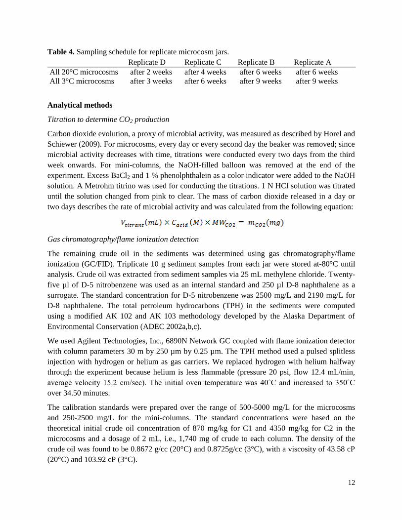
Table 4. Sampling schedule for replicate microcosm jars.

Replicate D Replicate C Replicate B Replicate A

All 20°C microcosms after 2 weeks after 4 weeks after 6 weeks after 6 weeks

All 3°C microcosms after 3 weeks after 6 weeks after 9 weeks after 9 weeks

Analytical methods

Titration to determine CO2 production

Carbon dioxide evolution, a proxy of microbial activity, was measured as described by Horel and

Schiewer (2009). For microcosms, every day or every second day the beaker was removed; since

microbial activity decreases with time, titrations were conducted every two days from the third

week onwards. For mini-columns, the NaOH-filled balloon was removed at the end of the

experiment. Excess BaCl2 and 1 % phenolphthalein as a color indicator were added to the NaOH

solution. A Metrohm titrino was used for conducting the titrations. 1 N HCl solution was titrated

until the solution changed from pink to clear. The mass of carbon dioxide released in a day or

two days describes the rate of microbial activity and was calculated from the following equation:

Gas chromatography/flame ionization detection

The remaining crude oil in the sediments was determined using gas chromatography/flame

ionization (GC/FID). Triplicate 10 g sediment samples from each jar were stored at-80°C until

analysis. Crude oil was extracted from sediment samples via 25 mL methylene chloride. Twenty-

five µl of D-5 nitrobenzene was used as an internal standard and 250 µl D-8 naphthalene as a

surrogate. The standard concentration for D-5 nitrobenzene was 2500 mg/L and 2190 mg/L for

D-8 naphthalene. The total petroleum hydrocarbons (TPH) in the sediments were computed

using a modified AK 102 and AK 103 methodology developed by the Alaska Department of

Environmental Conservation (ADEC 2002a,b,c).

We used Agilent Technologies, Inc., 6890N Network GC coupled with flame ionization detector

with column parameters 30 m by 250 µm by 0.25 µm. The TPH method used a pulsed splitless

injection with hydrogen or helium as gas carriers. We replaced hydrogen with helium halfway

through the experiment because helium is less flammable (pressure 20 psi, flow 12.4 mL/min,

average velocity 15.2 cm/sec). The initial oven temperature was 40˚C and increased to 350˚C

over 34.50 minutes.

The calibration standards were prepared over the range of 500-5000 mg/L for the microcosms

and 250-2500 mg/L for the mini-columns. The standard concentrations were based on the

theoretical initial crude oil concentration of 870 mg/kg for C1 and 4350 mg/kg for C2 in the

microcosms and a dosage of 2 mL, i.e., 1,740 mg of crude to each column. The density of the

crude oil was found to be 0.8672 g/cc (20°C) and 0.8725g/cc (3°C), with a viscosity of 43.58 cP

(20°C) and 103.92 cP (3°C).

13

The total area of the chromatogram was taken into account when calculating the concentration of

crude oil present in the sediments for days 0, 14, 28 and 42 at 20°C and for days 0, 21, 42 and 63

at 3°C.

Gas chromatography/mass spectroscopy

For microcosms, volatile compounds released by crude oil were trapped in 5 g of activated

carbon suspended in a mesh bag in the jar. In weekly intervals, the activated carbon was removed

from the microcosms. To extract hydrocarbons from the activated carbon, 0.22 g of activated

carbon was put in a GC vial and 1.5 mL of carbon disulfide was added with 25 µl of D-5

Nitrobenzene as an internal standard to verify the efficiency of the extraction. The concentration

of the internal standard was 2500 mg/L.

For mini-columns, 0.5 g of activated carbon was measured into individual GC vials; the vials

were labeled and stored at -80°C. When the samples were ready for analysis, the vials were

allowed to defrost. One mL of carbon disulfide was added to each vial. Five µL of the internal

standard of 2500 mg/L of heating fuel in carbon disulfide was added to each vial. The vials were

immediately placed on the GC-MS for analysis.

To determine the gasoline range organics for microcosms and mini-columns, we modified the

AK 102 (ADEC 2002) method. The GC-MS used was an Agilent Technologies 6890N Network

with a JW 123-1062 and a 60 m by 250 µm by 0.25 µm column. The volatile organic compounds

(VOC) method uses a splitless injection with helium as the carrier gas (pressure 9 psi, flow 1.6

mL/min, average velocity 3.2 cm/sec). The oven was set at an initial temperature of 150°C and

increased to 350°C, over 16.50 minutes.

A calibration curve was established using standards over a range from 250 to 5000 mg/L. The

total area of the gasoline range was used, and the concentration of the released volatiles was

calculated based on the calibration curve. The D-5 Nitrobenzene had an affinity for the activated

carbon that was used in this study and this compromised the recovery efficiency for the volatiles.

The same procedure and data analysis were followed for experiments at both 20°C and 3°C.

When analyzing samples from mini-columns, the GC/MS encountered some technical

difficulties (samples were skipped over and not analyzed or only analyzed for an insufficient

time period) leaving over a quarter of the data unusable. Therefore, no results are available for

volatiles in the mini-columns.

Most probable number

Crude oil is degraded by microbes present in the sediments. The number of crude oil-degrading

microorganisms was calculated by using the most probable number (MPN) method. This

technique follows a standard protocol where triplicate 1 gram sediment samples from each jar

were taken in a falcon tube. Ten mL of 1% sodium pyrophosphate solution along with 3-4 grams

of sterile glass beads were added to those falcon tubes. This mixture was put on the shaker table

for 1 hour, after which the tube was allowed to stand for half an hour. Then, in each well of 96-

14

well microtiter plates, 180 µl of Bushnell growth medium, 20 µl of microbial suspension (after

1.5 hours) and 5 µl of filtered crude oil (carbon source) was added. Three replicates (i.e., 3 rows)

were performed for each sample, each row with increasing dilution from left to right; including

one control row without a carbon source and one control row containing no microbial suspension

(Figure 3). The 96-well plates were incubated for 14 days at room temperature. Five µl of 2-(4-

iodophenyl)-3-(4-nitrophenyl)-5-phenyl-2H-tetrazolium (INT) dye was added to each well on the

15th

day, and again the plates were incubated for 24 hours in the dark. Positive growth as

indicated by a change in color (pink) was noted on the 16th

day. The experimental procedure was

followed for 20°C.

The observed data were entered into the EPA MPN calculator software to determine the number

of microbes present in the sediments. The EPA MPN calculator provides a specific concentration

in MPN/mL based on the number of positive wells.

However, there was some inconsistency in recording the color change on day 16, as the crude oil

formed a dark layer on top of each well, hindering the correct color change identification.

Therefore, the carbon source and incubation temperature were changed for low-temperature

experiments.

For the experimental study at 3°C, diesel was used as the carbon source. Since diesel is clear in

color, it was expected that this would enable better visual inspection. Wrenn and Venosa (1996)

demonstrated success using separate carbon sources to provide alkanes and PAHs as an

alternative to using only crude oil. The incubation temperature was kept at 10°C as this was

expected to result in a reasonable number of microbes for the reading on day 16.

Unfortunately, no reasonable MPN results were obtained due to low-temperature dormancy of

the microbes and poor conditions for visual inspection. Therefore, the MPN results will not be

discussed in the results section but are included in the Appendix.

Figure 3. MPN plate with crude oil as a carbon source.

15

Mini-column studies

The purpose of these experiments was to study biodegradation and transport of crude oil through

the sediment. Mini-columns were filled with sediment, crude oil was added, and several flushing

cycles were performed to simulate tidal action. After different experimental durations, the

petroleum hydrocarbons at different depths within the column were measured. The amount of

hydrocarbons evaporated was determined by measuring volatiles collected in activated carbon,

and the amount of CO2 released was determined by titrations of NaOH. Temperature, sediment

type, and the addition of liquid or solid fertilizer varied for the experiment.

Construction of mini-columns

Mini-columns were constructed using PVC pipe, as shown in Figure 4. A 1½ inch ABS PVC-

pipe was cut into 18-inch sections, each with an ABS adapter and a threaded plug fitting attached

to each end. A threaded ¼ in. hole was drilled into the plug fitting and a barbed nylon national

pipe thread was threaded into place. ABS cement was then used to seal the adapter fitting and

barbed nylon into place to ensure no water could leak out.

Figure 4. Column design used in the experiment.

Experimental design

Two preliminary experiments were performed to determine whether the frequency or number of

flushes was most influential in moving crude oil through the profile. The first experiment

involved varying the time between each flush, with the same number of flushes (six) in each

experiment. Three setups were compared; the first was a 6-hour study where the system was

flushed every hour. The second was over 48 hours, and the system was flushed every 8 hours.

The latter took 72 hours, and the system was flushed every 12 hours. The second experiment

varied the number of flushes using a standard time of 12 hours between flushes to reflect ocean

tidal cycles. As a 3-day trial had already been run, two additional studies were run for durations

of 6 and 12 days, with a total of 12 and 24 flushes, respectively. It was concluded that the

number of flushes had a greater impact on the overall movement of the oil than did time between

flushing

The titration data showing the amount of CO2 released produced interesting results. There was no

difference in the release of CO2 between the control column and the columns with crude oil

added. Two possible explanations for the relatively high respiration in the control and the low

16

respiration in columns with crude oil are (1) a carbon source may have been present in the soil,

and (2) the liquid fertilizer was rinsed out too fast to have an impact. For these reasons, it was

decided to conduct additional experiments of 18-day duration and with solid fertilizer as shown

in Table 5. These experiments were run for 3, 6, 12 and 18 days, with flushes every 12 hours.

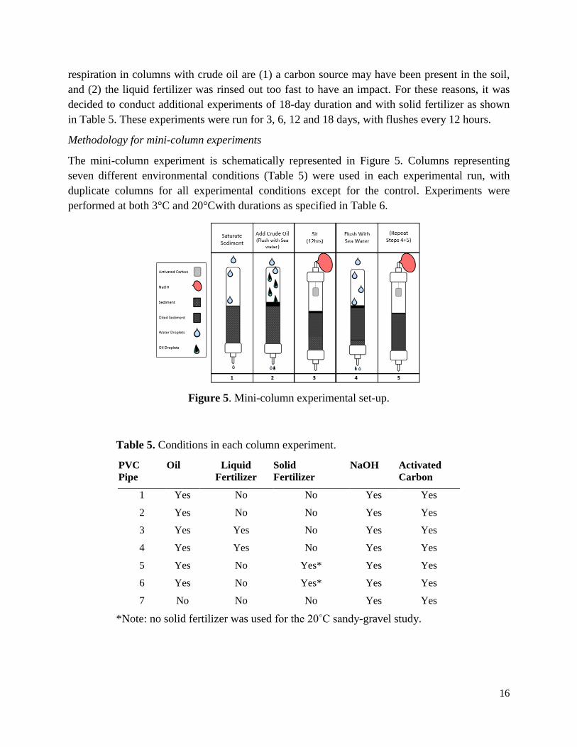
Methodology for mini-column experiments

The mini-column experiment is schematically represented in Figure 5. Columns representing

seven different environmental conditions (Table 5) were used in each experimental run, with

duplicate columns for all experimental conditions except for the control. Experiments were

performed at both 3°C and 20°Cwith durations as specified in Table 6.

Figure 5. Mini-column experimental set-up.

Table 5. Conditions in each column experiment.

PVC

Pipe

Oil Liquid

Fertilizer

Solid

Fertilizer

NaOH Activated

Carbon

1 Yes No No Yes Yes

2 Yes No No Yes Yes

3 Yes Yes No Yes Yes

4 Yes Yes No Yes Yes

5 Yes No Yes* Yes Yes

6 Yes No Yes* Yes Yes

7 No No No Yes Yes

*Note: no solid fertilizer was used for the 20˚C sandy-gravel study.

17

The procedure for the mini-column experiment follows:

1. Seven PVC pipes were filled with enough sediment mixture to make 12-inch sections and

placed on a shaker table to pack the column down to simulate ocean beaches.

2. The sediment was saturated from the top with water. Once saturated the bottom of the

column was opened to drain excess water.

3. Two mL of crude oil was introduced from the top to PVC pipes 1, 2, 3, 4, 5 and 6.

4. Twenty mL of fertilizer (N=300 mg/mL) was then added to column 3 and 4. The fertilizer

solution was prepared by dissolving a solid 20-20-20 fertilizer (20% nitrogen from 20%

ammonia, 30% nitrate, and 50% urea) in water.

5. 0.5 g of solid fertilizer of the same type was added to column 5 and 6 to achieve a dosage

of 600 mg/ of nitrogen. PVC pipe 7 was used as a control with no fertilizer or oil added.

6. Fifty mL of artificial sea water (prepared using Instant Ocean Aquarium Salt to

salinity=30 g/L) was added from the top and allowed to drain out completely. Once

drained, the bottom valve was shut allowing no more water or oil to exit the column.

7. A “tea bag” filled with ~1.5 g of activated carbon was suspended in the tube air space.

The same “tea bag” would be used for the entire course of each experiment, to ensure that

the final reading would be total volatiles released over the specific time frame.

8. A clear balloon filled with 20 mL of 1 N NaOH solution was attached to the cap of the

PVC-pipe to ensure that no air could escape. The same NaOH was used for the entire

experiment and, after the 18 day experiment, it was clear from titrations that the NaOH

was still able to absorb CO2, so no loss of CO2 was believed to occur.

9. The top of the column was sealed using plumbers tape wrapped around the thread cap

tightly fitted to the top of the column so no air could escape.

10. After allowing the system to sit for 12 hours, the NaOH balloon and activated carbon

were removed. Steps 7-12 were repeated for the remaining flush cycles with experimental

durations of 3, 6, 12 or 18 days (Table 6).

Table 6. Column flush cycle.

Hours between flushes Number of Flushes Number Days

12 6 3

12 12 6

12 24 12

12 36 18

Total petroleum hydrocarbon remaining in the sediment, released CO2, captured in NaOH

solution (indicating hydrocarbon mineralization) and volatilized hydrocarbons captured in

activated carbon were analyzed (see above: Analytical methods). After the last cycle, the bottom

end of the mini-column PVC pipe was opened and allowed to sit for 30 minutes. The NaOH

balloon and activated carbon were removed for analysis. One composite sediment sample of

approximately 10 g was taken from the top, middle and bottom of each column. The samples

were stored in amber vials at -80˚C until analysis.

18

Wave tank study

A wave tank was used in an observational study to simulate how crashing waves on the shore

affect the movement of the oil through the sediment horizon. A 5×1.5×2 ft. Plexiglas tank was

fitted with a divider so sandy-gravel and pebble sediment types could be evaluated

simultaneously under identical conditions. Sediment was placed into the tank creating a slope of

approximately 30 degrees. The sediment was approximately 12 inches high and extended 20

inches on the tank’s bottom (Figure 6).

Figure 6. Wave tank schematic.

The tank was filled with 10 gallons of artificial salt water mixture. After allowing the water to

saturate the sediment (~ 30 min), a wave-maker (Jebao WP-40, 900 to 3400 GPH) was used to

generate a consistent wave pattern. Once the wave generation stabilized, 20 mL of crude oil was

added to one end of the tank, and 5 mL was added straight to the shoreline. The 20°C and 3°C

experiments were conducted over three day periods with continuous wave action. At the end of

the study, the wave simulator was turned off. After 30 min, the water was slowly drained from

the tank. Samples were collected but could not be analyzed due to water saturation; drying them

would have resulted in too much hydrocarbon loss. Therefore, this study was strictly

observational, and results are presented in the Appendix.

RESULTS AND DISCUSSION

Microcosm experiments

The rate of crude oil degradation for different salinities and crude oil concentration was assessed

as carbon dioxide production, loss of volatile compounds, and quantity of crude oil remaining in

the sediments. Microcosms were run for six weeks for 20°C treatments, and nine weeks for 3°C

treatments; all used subsamples of the same sandy-gravel sediment. Seven condition scenarios (3

controls and 4 experimental) were executed for each temperature and experimental duration.

Condition variables are described by the following abbreviations: C0 specifies that no crude oil

was added, C1 stands for a low crude oil concentration (1 mL/kg), C2 indicates high crude oil

concentration (5 mL/kg), S1 refers to low salinity (30 g/L, as present in Beaufort and Chukchi

sea) and S2 refers to a high salinity (35 g/L, as common worldwide) (Table 2). Abbreviation

pairs represent condition combinations.

19

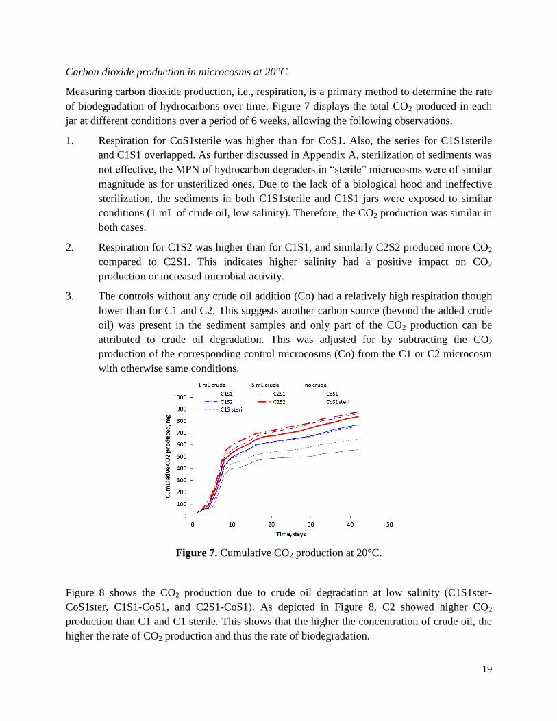
Carbon dioxide production in microcosms at 20°C

Measuring carbon dioxide production, i.e., respiration, is a primary method to determine the rate

of biodegradation of hydrocarbons over time. Figure 7 displays the total CO2 produced in each

jar at different conditions over a period of 6 weeks, allowing the following observations.

1. Respiration for CoS1sterile was higher than for CoS1. Also, the series for C1S1sterile

and C1S1 overlapped. As further discussed in Appendix A, sterilization of sediments was

not effective, the MPN of hydrocarbon degraders in “sterile” microcosms were of similar

magnitude as for unsterilized ones. Due to the lack of a biological hood and ineffective

sterilization, the sediments in both C1S1sterile and C1S1 jars were exposed to similar

conditions (1 mL of crude oil, low salinity). Therefore, the CO2 production was similar in

both cases.

2. Respiration for C1S2 was higher than for C1S1, and similarly C2S2 produced more CO2

compared to C2S1. This indicates higher salinity had a positive impact on CO2

production or increased microbial activity.

3. The controls without any crude oil addition (Co) had a relatively high respiration though

lower than for C1 and C2. This suggests another carbon source (beyond the added crude

oil) was present in the sediment samples and only part of the CO2 production can be

attributed to crude oil degradation. This was adjusted for by subtracting the CO2

production of the corresponding control microcosms (Co) from the C1 or C2 microcosm

with otherwise same conditions.

Figure 7. Cumulative CO2 production at 20°C.

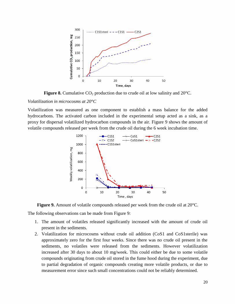
Figure 8 shows the CO2 production due to crude oil degradation at low salinity (C1S1ster-

CoS1ster, C1S1-CoS1, and C2S1-CoS1). As depicted in Figure 8, C2 showed higher CO2

production than C1 and C1 sterile. This shows that the higher the concentration of crude oil, the

higher the rate of CO2 production and thus the rate of biodegradation.

20

Figure 8. Cumulative CO2 production due to crude oil at low salinity and 20°C.

Volatilization in microcosms at 20°C

Volatilization was measured as one component to establish a mass balance for the added

hydrocarbons. The activated carbon included in the experimental setup acted as a sink, as a

proxy for dispersal volatilized hydrocarbon compounds in the air. Figure 9 shows the amount of

volatile compounds released per week from the crude oil during the 6 week incubation time.

Figure 9. Amount of volatile compounds released per week from the crude oil at 20°C.

The following observations can be made from Figure 9:

1. The amount of volatiles released significantly increased with the amount of crude oil

present in the sediments.

2. Volatilization for microcosms without crude oil addition (CoS1 and CoS1sterile) was

approximately zero for the first four weeks. Since there was no crude oil present in the

sediments, no volatiles were released from the sediments. However volatilization

increased after 30 days to about 10 mg/week. This could either be due to some volatile

compounds originating from crude oil stored in the fume hood during the experiment, due

to partial degradation of organic compounds creating more volatile products, or due to

measurement error since such small concentrations could not be reliably determined.

21

3. C1S1 sterile, C1S1 and C1S2 initially contained the same amount of crude oil and

consequently showed very similar release of volatiles, which was only substantial over

the first week and rapidly declined thereafter.

4. C2S1 and C2S2 also showed similar volatilization, as reflected in similar amounts of

hydrocarbons being present. Volatilization was very high in the initial week and rapidly

declined over the course of the experiment.

5. Salinity had no significant impact on volatilization.

Hydrocarbons remaining in sediments in microcosms at 20°C

Total petroleum hydrocarbons present in the sediments declined over time at 20°C as illustrated

in Figure 10.

Figure 10. Total petroleum hydrocarbons remaining in sediments at 20°C.

Total petroleum hydrocarbon changes showed the following trends:

1. The CoS1 control and CoS1 sterile series coincided, which can be explained by the fact

that sterilization was not successfully executed.

2. C1S1sterile, C1S1, and C1S2 also showed very similar results. Again, the fact that

sterilization was not effective explains the similar behavior of the “sterile” set-ups.

Salinity did not show a significant impact on TPH removal at low crude oil

concentrations.

3. C2S2 and C2S1 initially showed a difference in the amount of crude oil measured

initially though the same amount of crude oil was added for both. This could be either a

measurement error or an error when adding crude oil. TPH in C2S2 declined sharply and

then showed similar values as for C2S1, which makes it more likely that a measurement

error on day 1 occurred.

Hydrocarbon data showed a similar declining trend over time as volatile compounds in Figure 9.

Comparing Figures 8 through 10, the same result was observed; maximum oil removal was

22

observed at high crude oil concentration and high salinity. The percentage of crude oil removal

from the sediments over 6 weeks was:

% removal = 100 × (TPHday0 – TPHday42)/TPHday0

The removal percentages shown in Figure 11 increase with increasing concentration and salinity,

following the same trends as discussed above.

Figure 11. Percentage of TPH removal from sediments over 6 weeks at 20°C.

Carbon dioxide production in microcosms at 3°C

The cumulative respiration over time is shown in Figure 12, and the following observations can

be made from this figure.

1. CoS1 and CoS1sterile series (controls) are overlapping, which was due to ineffective

sterilization. Both show substantial CO2 production, in the same order of magnitude as

other experiments with crude oil addition, which suggests another carbon source was

present in the sediments. This matches observations made at 20°C. This can also be

confirmed by data shown in Figure 15, where organic carbon was found in the sediments,

even when no crude oil had been added.

2. The low crude oil concentration series C1S1 and C1S2 overlapped (no effect of salinity)

and show the highest CO2 production of all setups at 3°C.

3. All microcosms at the lower crude oil concentration, even the C1S1 sterile control

showed higher CO2 production than C2S2 and C2S1. This is unusual, typically CO2

production increases with higher substrate (hydrocarbon) concentration. This could be

because the microbes were not able to break down the complex compounds of crude into

CO2. Inhibition or toxicity may have occurred at the higher crude oil concentration.

4. C2S2 showed higher CO2 production compared to low salinity C2S1. Apparently higher

salinity had a positive impact on CO2 production for C2, as observed at 20°C.

23

Figure 12. Cumulative CO2 production at 3°C.

Figure 13 shows the CO2 production due crude oil mineralization for different concentrations at

low salinity. From C1 and C2 respiration values, the CO2 production for the control without

crude oil was subtracted to calculate the respiration due to crude oil mineralization. High crude

oil concentrations (C2) clearly led to lower CO2 production than for low crude oil concentration

(C1). At 3°C, the higher crude oil concentration apparently inhibited the process of CO2

production. Some initial negative values (shown as zero) were calculated since Co initially had

higher respiration than C1 or C2 in some cases. A possible explanation could be that crude oil

hindered oxygen supply.

Figure 13. Cumulative CO2 production due to crude oil for low salinity at 3°C.

Volatilization in microcosms at 3°C

The following observations can be made based on Figure 14, which presents the amount of

volatiles released from crude oil over 9 weeks at 3°C.

24

1. CoS1 control and CoS1 sterile volatilization values were insignificant for the first four

weeks. Since there was no crude oil present in the sediments, no volatiles were released

from the sediments.

2. In all setups with 1 mL crude oil (C1S1 sterile, C1S1 and C1S2), volatile compounds

released declined over time, with similar volatilization values for all three series.

3. Similarly, the two setups with the higher crude oil concentration, C2S1, and C2S2,

showed initially high volatilization with a decreasing trend, though some fluctuations

were observed especially around day 21.

4. Salinity had no significant impact on volatilization.

5. The amount of volatiles released increased with the amount of crude oil present.

Figure 14. Amount of volatile compounds released per week from the crude oil at 3°C.

Hydrocarbons remaining in sediments in microcosms at 3°C

Total petroleum hydrocarbons present in the sediments at 3°C declined over time as illustrated in

Figure 15. For data obtained at different crude oil concentrations, the following observations

were made.

1. TPH in the CoS1 control and CoS1 sterile were very low as expected. The small amount

of TPH measured may be due to measurement error or other carbon compounds

interfering with the measurement, as similarly observed for 20°C.

2. All setups at the lower crude oil concentration, i.e., C1S1 sterile control, C1S1, and C1S2

showed very similar and quite low TPH values, with little change over time. Salinity did

not show a significant impact at low crude oil concentrations. Sterilization also showed

no effect.

3. C2S2 and C2S1, which had the same higher concentration of crude oil, initially showed a

difference; however, TPH values for C2S2 declined sharply, eventually approaching

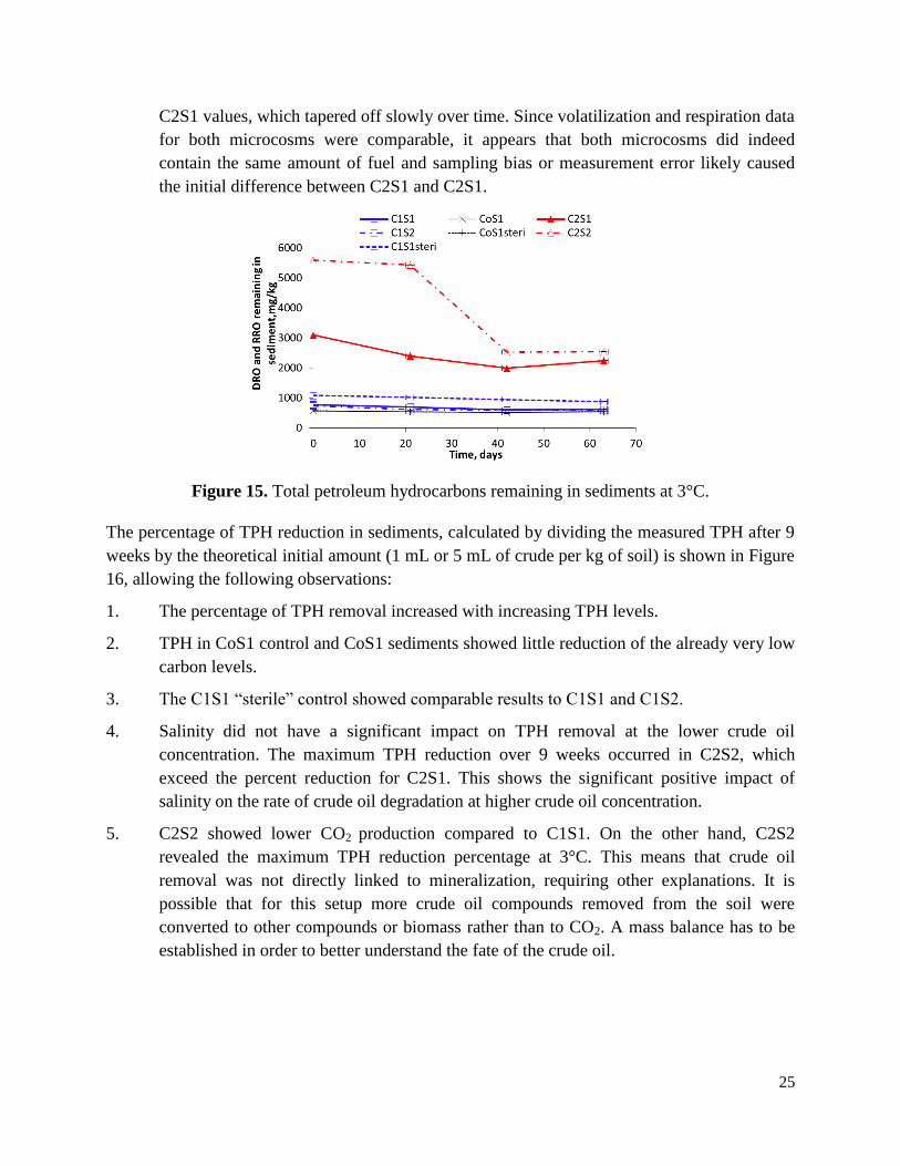
25

C2S1 values, which tapered off slowly over time. Since volatilization and respiration data

for both microcosms were comparable, it appears that both microcosms did indeed

contain the same amount of fuel and sampling bias or measurement error likely caused

the initial difference between C2S1 and C2S1.

Figure 15. Total petroleum hydrocarbons remaining in sediments at 3°C.

The percentage of TPH reduction in sediments, calculated by dividing the measured TPH after 9

weeks by the theoretical initial amount (1 mL or 5 mL of crude per kg of soil) is shown in Figure

16, allowing the following observations:

1. The percentage of TPH removal increased with increasing TPH levels.

2. TPH in CoS1 control and CoS1 sediments showed little reduction of the already very low

carbon levels.

3. The C1S1 “sterile” control showed comparable results to C1S1 and C1S2.

4. Salinity did not have a significant impact on TPH removal at the lower crude oil

concentration. The maximum TPH reduction over 9 weeks occurred in C2S2, which

exceed the percent reduction for C2S1. This shows the significant positive impact of

salinity on the rate of crude oil degradation at higher crude oil concentration.

5. C2S2 showed lower CO2 production compared to C1S1. On the other hand, C2S2

revealed the maximum TPH reduction percentage at 3°C. This means that crude oil

removal was not directly linked to mineralization, requiring other explanations. It is

possible that for this setup more crude oil compounds removed from the soil were

converted to other compounds or biomass rather than to CO2. A mass balance has to be

established in order to better understand the fate of the crude oil.

26

Figure 16. Percentage of TPH removal from sediments over 6 weeks at 3°C.

Carbon dioxide production in microcosms at both temperatures

Since 20°C experiments were conducted for 6 weeks and 3°C studies were carried out for 9

weeks, the results for both temperatures will be compared over 6 weeks. The following

observations can be made from Figure 17, which shows the cumulative CO2 production.

1. For each set of conditions, the CO2 production at 20°C was higher than at 3°C. These

results are consistent with Arrhenius principle, according to which biological activity

slows down at low temperatures. Therefore, more time will be required for the microbes

to mineralize crude oil at lower temperatures.

2. For both temperatures and both crude oil concentrations (C1S1 vs. C1S2, and C2S1 vs.

C2S2), respiration for S2 was slightly higher than for S1.

3. At 20°C, respiration was a little higher for C2 than for the corresponding C1 microcosms.

However, at 3°C respiration in C2 was lower than in C1. This indicates that higher crude

concentration inhibits the conversion of crude to CO2 at 3°C.

4. For both temperatures, C1S1sterile and C1S1 showed similar values, suggesting

incomplete sterilization.

Figure 17. Cumulative CO2 produced in 6 weeks at 20°C and 3°C.

27

Volatilization in microcosms at both temperatures

Figure 18 compares volatilization at both temperatures. The percentage volatilized was

calculated as described above. According to literature, volatilization is slower at low

temperatures. However, the data in the figure below show comparable volatilization percentages

for both temperatures, in some cases even higher volatilization at the lower temperature.

Figure 18. Percentage of volatile compounds released during 6 weeks at 20°C and 3°C.

Hydrocarbons remaining in sediments in microcosms at both temperatures

Figure 19 compares the percentage of total petroleum hydrocarbons removed from the sediments

at 20°C and 3°C. Similarly high removal percentages were achieved at 3°C as observed at 20°C.

At both temperatures, C2S2 showed the highest percentage decline of carbon in sediments,

which confirms the initial hypothesis that better removal is achieved at high salinity. Removal at

3°C exceeded 50% after 6 weeks.

Figure 19. Percentage of TPH removal from sediments over 6 weeks at 20°C and 3°C.

28

Mass balance of crude oil in microcosms at both temperatures

A mass balance was made for the carbon initially present as crude oil, based on carbon recovery

in the form of carbon dioxide, volatile compounds, total petroleum hydrocarbons present in the

sediments, and an unidentified “other” being the difference between the above three categories

and 100%.

The carbon from crude oil converted to CO2 was calculated after subtracting the Co control

values from the respiration for C1 and C2 samples. Since Co had some carbon content initially,

C1 and C2 should have the same initial natural carbon content contributing towards CO2 release.

To relate the mass of hydrocarbons consumed to the amount of CO2 produced in the experiment,

the following generic stoichiometric equation for mineralization of hydrocarbons applies

(Cunningham 2004).

For icosane, C20H42 as a representative TPH for the current study, the above equation can be

written as:

This means the mineralization of 282 mg of hydrocarbons (1 mole icosane) leads to the

production of 880 mg of carbon dioxide (20 moles), i.e., 0.32 mg crude were consumed per mg

of CO2 produced. In order to calculate what percentage of crude oil was converted to CO2 the

following equations were used:

For the amount of crude initially present (mcrude added), the theoretical value based on the volume

of crude oil added was used, i.e., 870 mg for C1 and 4350 mg for C2.

The following equation was used to calculate the % of carbon recovered as Volatile Organic

Compounds (VOC):

The percentage of Total Petroleum Hydrocarbons (TPH) remaining in the sediment was

calculated as:

These mass balance percentages provide a better understanding of what is actually happening

and how much CO2, VOC, and TPH were recovered under different environmental conditions.

29

Mass balances for both temperatures are compared in Figure 20, allowing the following

observations:

1. Mineralization (CO2) was the smallest of the fractions shown in the mass balance. The

mineralization percentage at 20°C was consistently higher than at 3°C. This conforms to

the common observation that microbial activity increases with temperature. At the higher

crude oil dosage, a smaller percentage was mineralized.

2. Volatilization was quite high. The percentage volatilized was a little higher at the lower

crude oil dosage. According to the literature, VOC release should slow down at low

temperature. However most microcosms, especially C1S1sterile, showed higher

volatilization at 3°C than at 20°C. VOC releases in other microcosms were similar for

both temperatures.

3. The remaining TPH percentage did not show a clear trend with respect to temperature.

4. At the lower crude oil concentration, recovery was >100 %, which may have been due to

the presence of some naturally occurring carbon source. The impact of that naturally

present carbon was less noticeable in the mass balance for the higher crude oil

concentration.

Figure 20. Mass balances of crude oil at 20°C and 3°C after 6 weeks. The graph shows fractions

mineralized (CO2), volatilized (VOC) and remaining in soil (TPH). Red line is at 100%.

Mini-column experiments

The purpose of these experiments was to understand the fate of crude oil in different shoreline

substrates. After describing results for sandy-gravel and pebble sediment, respectively, a

comparison of sandy-gravel versus pebble was presented. In each case, two temperatures and

different fertilizer types were compared to determine their effect on the fate of the crude oil.

30

For all of the above conditions (different sediment types, temperatures, and fertilizer

application), the crude oil degradation and transport were evaluated by measuring three

parameters: the concentration of crude oil throughout the column profile, the CO2 production,

and the release of hydrocarbon volatiles (data not shown due to analytical problems). Studies

performed over 3, 6, 12, and 18 days were compared to evaluate hydrocarbon movement in the

sediment over time.

It should be noted that for all graphs showing the variation of crude oil concentration, the control

columns are not included because the hydrocarbon concentration was consistently very low

(approx. 50 mg/kg) for all experiments.

Crude oil movement in sandy-gravel sediment

The sandy-gravel sediment was composed of coarse grain sand, with some gravel. The sandy-

gravel sediment was found to have a porosity of 0.359 with an expected oil penetration of 25 cm

(NOAA 2004). Figures 21 and 22 show the average crude oil concentration at different places in

the column for the 20°C and 3°C studies, respectively.

At 20°C, it is notable that all sandy-gravel columns follow the same general trend. A much

higher concentration of crude oil resided in the middle section of the column, about 6 inches

below the surface. This result is consistent with the classification as ESI 4, which has an

expected maximum oil penetration of 25 cm (NOAA 2002).

For most days, a higher concentration of crude oil was noted in the columns with no fertilizer

added. The crude oil concentration in the column with no fertilizer showed a consistent

downward trend over time for the top and middle of the column, with concentrations consistently

highest in the middle.

The liquid fertilizer follows the same trend with highest concentrations observed in the middle of

the column followed by the bottom of the column and lowest concentrations at the top. The

increase in TPH at the top of the column from day 3 to day 6 must have been a sampling error on

either day 3 or 6. There was an initial decline in TPH from 0 to 3 days, but from 3 to 12 days a

very little additional decline in crude oil concentration is seen. Therefore, it appears that the

addition of fertilizer does not have a significant impact on the degradation of crude oil after 3

days. This can be attributed to the fact that the fertilizer was in liquid form and most likely

washed through the entire column by day 3.

Crude oil concentrations at 3°C did not follow the clear trend as seen at 20°C. In unfertilized

columns, the maximal crude oil concentration occurred in the middle of the column. It also

appears that past day 6, there was no significant decrease in crude oil concentration at the top of

the column, with nearly identical concentrations on day 6, 12, and 18, indicating that no further

movement from the top of the column occurred through the sediment. Over time, the average

crude oil concentrations slowly decreased. Although there is a downward trend, removal did not

occur to the same extent as at 20°C.

31

Figure 21. TPH concentration at different depths after 3-12 days in sandy-gravel at 20°C.

Figure 22. TPH concentration at different depths after 3-18 days in sandy-gravel at 3°C.

In columns with liquid or solid fertilizer, either the top or the middle of the column showed the

highest TPH concentrations. Similar to 20°C the crude oil concentrations decreased over time,

but it does not appear that fertilizer addition contributes to oil movement. With solid fertilizer,

average TPH concentrations decrease at a very slow rate. The concentration at the top of the

column remains consistently high. By day 18, the columns with solid fertilizer had the highest

crude concentration at any level.

Carbon dioxide release in sandy-gravel sediment

Figures 23 and 24 show the average cumulative amounts of CO2 that were released from each of

the columns over 3, 6, 12, and 18 days for 20°C and 3°C, respectively. Respiration data at 20°C

followed the generally expected trend, with a steady increase in CO2 produced over time. Day 3

and 6 show very similar respiration for all 3 conditions, i.e., there was no noticeable effect of

crude oil or nutrient addition. The similarly high CO2 release without crude oil addition indicates

that there must have already been a carbon source present in the soil; a similar finding was made

by Sharma, 2015. For the first 6 days, the microbes present in the soil may still have been

32

utilizing the original carbon source and had not yet begun to degrade the crude oil. By day 12,

the original carbon source may have been used up, and the microbes moved on to the crude oil

allowing them to release an additional 20-40 mg of CO2. It is interesting to note that the liquid

fertilizer does not appear to have as positive an impact on the release of CO2, as was expected.

As mentioned before, this could be due to the fertilizer being flushed out of the system early on,

and therefore no longer being present by day 12 when crude oil utilization started. It should be

mentioned that throughout the experiment, the columns were flushed with sea water, which

means that along with a higher salinity, there were also nutrients present in the water. So it is

possible that the simple addition of sea water to the system was enough to stimulate the

microbes. It is still unclear why the columns with no fertilizer released so much more CO2.

Figure 23. Cumulative CO2 released from sandy-gravel at 20°C.

Figure 24. Cumulative CO2 released from sandy-gravel at 3°C

The CO2 production from sandy-gravel at 3°C showed a similar trend as in the 20°C study,

where independent of fertilization and crude oil addition almost the same amount of CO2 was

released for day 3 and 6 (in the 20°C study a nearly identical release was also seen at day 12). It

was not until day 18 that a significant spike in CO2 release due to crude oil degradation was seen.

This longer lag time can be attributed to the lower temperature. It is known that as temperature

decreases, microbes slow down their metabolic rate and, therefore, do not need to consume their

energy source at as quickly (Horel, 2009). While it is higher than on day 12, it is important to

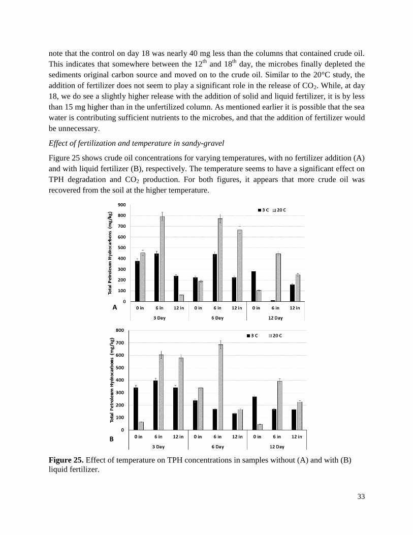
33

note that the control on day 18 was nearly 40 mg less than the columns that contained crude oil.

This indicates that somewhere between the 12th

and 18th

day, the microbes finally depleted the

sediments original carbon source and moved on to the crude oil. Similar to the 20°C study, the

addition of fertilizer does not seem to play a significant role in the release of CO2. While, at day

18, we do see a slightly higher release with the addition of solid and liquid fertilizer, it is by less

than 15 mg higher than in the unfertilized column. As mentioned earlier it is possible that the sea

water is contributing sufficient nutrients to the microbes, and that the addition of fertilizer would

be unnecessary.

Effect of fertilization and temperature in sandy-gravel

Figure 25 shows crude oil concentrations for varying temperatures, with no fertilizer addition (A)

and with liquid fertilizer (B), respectively. The temperature seems to have a significant effect on

TPH degradation and CO2 production. For both figures, it appears that more crude oil was

recovered from the soil at the higher temperature.

Figure 25. Effect of temperature on TPH concentrations in samples without (A) and with (B)

liquid fertilizer.

A

A

m

i

x

e

d

s

a

n

d

/

p

e

b

b

l

e

s

a

B

A

m

i

x

e

d

s

34

At 20°C, there is a fairly clear trend of crude oil moving through the column, with only little

TPH present in the top layer after day 6. TPH concentrations overall decreased with time but

were nevertheless on average still higher than at 3°C. At the lower temperature, the concentration

after 3 days was already relatively low and decreased only slightly over time. One explanation

for this apparently quick loss of TPH in the first three days at 3°C could be that an initial

movement of crude oil through the system led to the removal of crude oil, but, considering the

lower viscosity at low temperatures, that situation seems unlikely. Another possible explanation

could be that the 20°C samples were extracted and analyzed within a week of the completion of

the experiment. Whereas, the 3°C samples were stored in the -80°C freezer for about three weeks

(up to 31 days), before extraction and then due to machine malfunction had to be stored for

another four weeks (up to 40 days) before analysis could be completed. While extraction and

analysis were both within the required time frames, they did have a slightly lower crude oil

recovery from the soil, but still within the recommended recovery rate.

Figure 26 shows how the temperature affected the release of CO2 in sandy-gravel sediment. For

any time period, there was a higher release at 20°C than at 3°C. It is normal for microbes to be

more active at higher temperatures than at lower temperatures. Nevertheless, this is interesting as

the native microorganisms would be more adapted to low temperatures and perform well. The

majority of the Arctic rarely reaches air temperatures of 20°C, and the average summer

temperature is around 3°C. It can be extrapolated from the data that if an 18 day study at 20°C

had been completed, the CO2 release would have been greater than the 110 mg released at 3°C.

Figure 26. Effect of temperature on the release of CO2 from sandy-gravel with liquid fertilizer.

Crude oil movement in pebble sediment

The pebble sediment used was characteristic of ESI 5 sediments, which are comprised of a

mixture of pebbles with some sand. The pebble sediment porosity was determined to be 0.307, a

medium to high permeability with a high chance of oil penetration up to 50 cm (NOAA 2002).

Figures 27 and 28 show the average crude oil concentration at different locations in the column

for the 20°C and 3°C studies, respectively. A similar trend is seen at both temperatures, with a

higher crude oil concentration at the top (0 in) and the bottom (12 in), and the lowest

concentration in the middle.

35

Figure 27. TPH concentration at different depths after 3 - 18 days in pebble sediment at 20°C.

Figure 28. TPH concentration at different depths after 3 -18 days in pebble sediment at 3°C.

At 20°C, it appears that the movement of crude oil is consistent with the ESI 5 rating. Already on

day 3, a high concentration of crude oil was observed not only at the top but also at the bottom of

the column, indicating that significant transport had occurred during that short time period, i.e.,

the crude oil moved freely through the column. By day 6, the concentration at all levels, but

especially at the top had decreased, indicating that, the majority of crude oil (~ 75 mg/kg remain)

had been removed from both the top and middle layers of the column. This removal could have

been due to volatilization and/or biodegradation (discussed below). The upper two layers showed

a further slight decrease in concentration over the next 12 days, with a residual concentration of

approximately 50 mg/kg. At the bottom of the column, a relatively high concentration was still

36

present at day 6 and 12, indicating some pooling may have occurred. By day 18, the entire

column exhibited the same low crude oil concentration, i.e., the majority of crude oil was

removed from the system, and the soils approached the TPH concentrations in the control

without fuel addition (approx. 50 mg/kg). TPH removal from the bottom layer may have been

due to crude oil slowly being washed out of the column over time. In situ, crude oil may be

washed back out into the ocean.

The same trend is seen at 3°C. The top and bottom of the column had a very high concentration

at day 3. At the top, this concentration dropped by day 6 to about 50 mg/kg and remained at that

level for the remainder of the study. After three days, the middle of the column showed

concentrations (100 mg/kg) that were lower than at the top or bottom. Over the next 12 days,

concentrations slowly decreased to a final concentration of 50 mg/kg. By day 18, this pooling

effect was no longer exhibited, and the entire column exhibited the same generally low

concentration of 50 mg/kg which is consistent with the control concentration. This means, at the

lower temperature, crude oil had been largely removed from the column over the 18-day

duration. As in the 20°C pebble study, the addition of fertilizers did not cause a large effect on

the movement of crude oil through the column. However, at 3°C, it appears the solid fertilizer

enabled TPH removal at a slightly faster rate. The liquid fertilizer also had this impact, but not to

the same degree as the solid fertilizer.

Carbon dioxide release in pebble sediment

Figures 29 and 30 show the amount of CO2 that was released (average of duplicate columns)

over 3, 6, 12, and 18 days for 20°C and 3°C, respectively. Respiration data at 20°C followed the

general trend that was seen in the sandy-gravel sediment. Compared to sandy-gravel, where for

the first 6 days all conditions showed comparable results (i.e., no effect of fertilizer or crude oil),

we see this trend at day 12 for the pebble sediment. Only on day 18, the effect of crude oil

mineralization on overall CO2 production becomes noticeable. Lower microbial numbers present

in the pebble sediment offers one explanation for this consistent release extending as far as day

12. A lower microbial population could be sustained by the original carbon source for a greater

amount of time and take longer before utilizing the crude oil. The reason why fewer microbes

might be present has to do with the structure of the sediment. Due to the greater porosity there is

a larger amount of air space in the sediment and a smaller surface area of the sediment grains.

Microbes, in general, favor lower porosity sediments, where they can be in contact with a greater

amount of resources. If large gaps exist, the microbes additionally encounter the risk of being

flushed out of the system.

The addition of fertilizer does appear to have had a fairly significant effect on the release of CO2.

Over time, the addition of both liquid and solid fertilizer increased the amount of CO2 being

produced. It appears that the solid fertilizer was more effective than the liquid fertilizer. By day

6, the columns with fertilizer released almost 20 mg (solid) and 10 mg (liquid) more CO2. At day

18 the fertilized columns released 40 mg (solid) and 20 mg (liquid) respectively more than the

unfertilized column, showing that fertilizer, in fact, facilitates CO2 production.

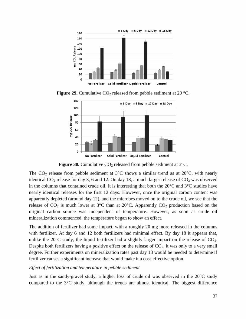
37

Figure 29. Cumulative CO2 released from pebble sediment at 20 °C.

Figure 30. Cumulative CO2 released from pebble sediment at 3°C.

The CO2 release from pebble sediment at 3°C shows a similar trend as at 20°C, with nearly

identical CO2 release for day 3, 6 and 12. On day 18, a much larger release of CO2 was observed

in the columns that contained crude oil. It is interesting that both the 20°C and 3°C studies have

nearly identical releases for the first 12 days. However, once the original carbon content was

apparently depleted (around day 12), and the microbes moved on to the crude oil, we see that the

release of CO2 is much lower at 3°C than at 20°C. Apparently CO2 production based on the

original carbon source was independent of temperature. However, as soon as crude oil

mineralization commenced, the temperature began to show an effect.

The addition of fertilizer had some impact, with a roughly 20 mg more released in the columns

with fertilizer. At day 6 and 12 both fertilizers had minimal effect. By day 18 it appears that,

unlike the 20°C study, the liquid fertilizer had a slightly larger impact on the release of CO2.

Despite both fertilizers having a positive effect on the release of CO2, it was only to a very small

degree. Further experiments on mineralization rates past day 18 would be needed to determine if

fertilizer causes a significant increase that would make it a cost-effective option.

Effect of fertilization and temperature in pebble sediment

Just as in the sandy-gravel study, a higher loss of crude oil was observed in the 20°C study

compared to the 3°C study, although the trends are almost identical. The biggest difference

38

between the two temperatures was seen at day 3. However, by day 6 there was no real

discernable difference between the two studies. It appears that crude oil movement in pebble

sediment is not greatly affected by the change in viscosity and available pore size as was seen in

the sandy-gravel studies. This makes sense, as pebble sediments generally have a much larger

pore size, which allows water to drain quickly through the system.

In an environment with no fertilizer addition (Figure 31), the TPH concentrations in the sediment

are generally slightly lower at 20°C than at 3°C. This means at the warmer temperature a slightly

greater loss of crude oil from the system takes place, especially during the first days; however,

there was no significant difference between TPH at 3°C and 20°C. In contrast to the sandy-

gravel sediment, a much smaller difference between the two temperatures was observed. Pebble

sediment has a much larger pore space, which allows for the crude oil to penetrate more freely. It

is apparent that temperature had no significant impact on the movement of crude oil. Figure 32

shows the movement of oil in the presence of fertilizer. Just as with the previous figure,

temperature does not appear to have a significant impact on the movement of crude oil.

Figure 31. Temperature effects on crude oil movement in pebble sediment with no fertilizer.

Figure 32. Temperature effects on crude oil movement in pebble sediment with fertilizer.

39

Respiration

Figure 33 illustrates the release of CO2 and its dependency on temperature. The graph shows

CO2 production for solid fertilizer (light lines) and liquid fertilizer (dark lines) as a function of

time. For the first six days, the release of CO2 is nearly identical for all temperatures and

fertilizers. At day 12, we begin to see a significantly higher release at 20°C. Recall that it was

concluded that, at day 12, the organisms had finally consumed the originally present natural

carbon source and had moved on to the crude oil. This caused a significant increase in CO2

release, especially at 20°C. At day 18, it was very clear that the warmer temperature showed a

much greater release of CO2 over time.

This trend makes sense because microbes require a higher amount of substrate at warmer

temperatures and more readily degrade contaminants due to increased metabolic rates. It can be

concluded that over the course of the first 12 days, as long as respiration was due to the natural

carbon source, the temperature had no significant impact. However, once the microbes had to

move to a new foreign substrate, the higher temperature led to a faster mineralization rate.

Figure 33. Temperature effects on the release of CO2 from pebble sediment with fertilizer.

Comparison of sediment types at 20 °C

Figures 34 A and B show the distribution of crude oil in the column at 20°C, for both sediment

types with no fertilizer addition. As already discussed above, the sandy-gravel sediment

accumulated oil in the middle of the column, whereas pebble sediment showed a higher

concentration initially at the top and bottom of the column. In a natural environment, it appears

that crude oil would remain in the sandy-gravel sediment for a much longer time frame. By day

6, the oil concentrations in pebble sediment have decreased significantly, where sandy-gravel

contained 700 mg/kg or 10 times as much crude oil as the pebble sediment in the middle section.

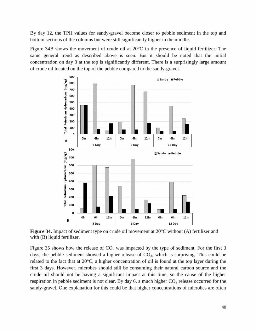
40

By day 12, the TPH values for sandy-gravel become closer to pebble sediment in the top and

bottom sections of the columns but were still significantly higher in the middle.

Figure 34B shows the movement of crude oil at 20°C in the presence of liquid fertilizer. The

same general trend as described above is seen. But it should be noted that the initial

concentration on day 3 at the top is significantly different. There is a surprisingly large amount

of crude oil located on the top of the pebble compared to the sandy-gravel.

Figure 34. Impact of sediment type on crude oil movement at 20°C without (A) fertilizer and

with (B) liquid fertilizer.

Figure 35 shows how the release of CO2 was impacted by the type of sediment. For the first 3

days, the pebble sediment showed a higher release of CO2, which is surprising. This could be

related to the fact that at 20°C, a higher concentration of oil is found at the top layer during the

first 3 days. However, microbes should still be consuming their natural carbon source and the

crude oil should not be having a significant impact at this time, so the cause of the higher

respiration in pebble sediment is not clear. By day 6, a much higher CO2 release occurred for the

sandy-gravel. One explanation for this could be that higher concentrations of microbes are often

41

present in finer grained material. Additionally, the concentration of crude oil in sandy-gravel was

higher, i.e., an increased amount of carbon source was available to the microbes.

Figure 35. Impact of sediment type on CO2 release at 20°C with liquid fertilizer.

Comparison of sediment types at 3°C

Figures 36A and B show the crude oil distribution at 3°C, without and with liquid fertilizer

addition, respectively. A similar trend as seen at 20°C is shown. There is higher crude oil

concentration for pebble sediment over the first 3 days. However, there is a smaller difference

between the concentration levels over time. From day 6 on, the crude oil concentration at the top

and middle in sandy-gravel was a multiple of that for pebble. Sandy-gravel and pebble showed

similar concentrations at the bottom of the columns, with a decreasing trend over time.

Different results were observed with the addition of solid fertilizer. Unlike previous results,

Figure 36C shows that, after 3 days, sandy-gravel had a much higher TPH concentration on the

top than pebble. Concentrations in pebble were extremely low after the first 3 days in the top and

middle sections of the column, with the highest crude oil concentrations at the bottom of the

column, where it also reached background (2 mg) levels after 18 days. By day 6 similar trends as

for the other fertilization regimes are shown, with lower concentrations in pebble sediment, and

TPH values in sandy-gravel remaining relatively high in the top and middle sections.

42

Figure 36. Impact of sediment type on crude oil movement at 3°C without fertilizer (A), with

liquid fertilizer (B), and with solid fertilizer (C).

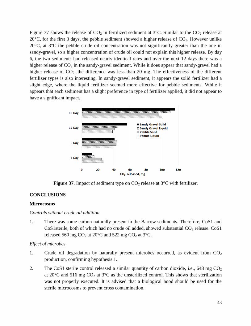
43

Figure 37 shows the release of CO2 in fertilized sediment at 3°C. Similar to the CO2 release at

20°C, for the first 3 days, the pebble sediment showed a higher release of CO2. However unlike

20°C, at 3°C the pebble crude oil concentration was not significantly greater than the one in

sandy-gravel, so a higher concentration of crude oil could not explain this higher release. By day

6, the two sediments had released nearly identical rates and over the next 12 days there was a

higher release of CO2 in the sandy-gravel sediment. While it does appear that sandy-gravel had a

higher release of CO2, the difference was less than 20 mg. The effectiveness of the different

fertilizer types is also interesting. In sandy-gravel sediment, it appears the solid fertilizer had a

slight edge, where the liquid fertilizer seemed more effective for pebble sediments. While it

appears that each sediment has a slight preference in type of fertilizer applied, it did not appear to

have a significant impact.

Figure 37. Impact of sediment type on CO2 release at 3°C with fertilizer.

CONCLUSIONS

Microcosms

Controls without crude oil addition

1. There was some carbon naturally present in the Barrow sediments. Therefore, CoS1 and

CoS1sterile, both of which had no crude oil added, showed substantial CO2 release. CoS1

released 560 mg CO2 at 20°C and 522 mg CO2 at 3°C.

Effect of microbes

1. Crude oil degradation by naturally present microbes occurred, as evident from CO2

production, confirming hypothesis 1.

2. The CoS1 sterile control released a similar quantity of carbon dioxide, i.e., 648 mg CO2

at 20°C and 516 mg CO2 at 3°C as the unsterilized control. This shows that sterilization

was not properly executed. It is advised that a biological hood should be used for the

sterile microcosms to prevent cross contamination.

44

Effect of crude oil concentration

1. Samples with higher crude oil concentration did not produce a significantly higher

amount of CO2 at either temperature. At 3°C, mineralization was even somewhat lower

for C2 than for C1, showing that complete mineralization is difficult in higher

contamination levels. Hypothesis 2a, which stated that a higher crude oil concentration

would increase the rate of mineralization was therefore proven wrong. In the mass

balance, relative mineralization percentages were lower for higher crude oil

concentrations confirming the initial hypothesis 2b.

2. VOC release was higher for C2 than for C1, i.e., more volatilization took place at higher

crude oil dosages, confirming hypothesis 3. However, the volatilization percentage was

lower for C2.

3. At higher crude oil dosages, more TPH remained in the sediments, both in absolute and

relative terms, confirming hypothesis 4.

Effect of temperature

1. Temperature played an important role in mineralization of crude oil. Higher CO2

production was observed at 20°C, than at 3°C, confirming hypothesis 5.

2. Also, the amount of TPH remaining in the sediment was higher at the lower temperature,

especially for high fuel dosages, confirming hypothesis 6 that higher temperatures

increase the microbial activity and lead to better crude oil removal.

3. Surprisingly, similar VOC production was noted for both temperatures, contradicting

hypothesis 7; literature describes that volatilization is lower at low temperatures.

Effect of Salinity

1. According to hypothesis 8, salinity has a positive impact on hydrocarbon degradation

rates, which was confirmed by the results at 20°C and 3°C. At both temperatures, S2

samples displayed higher respiration and volatilization as well as lower TPH. Literature

supports that at a high temperature increased salinity leads to higher oil degradation rates.

Based on the present research it can be concluded that the same effect can be seen at

lower temperatures.

Mass balance

1. According to the mass balance, only a small fraction was mineralized, most TPH removal

was due to volatilization rather than biodegradation.

2. Overall it can be concluded that environmental factors like temperature, crude oil volume

and salinity all impact the rate of crude oil degradation in laboratory experiments and are

expected to do so in real oil spill accidents.

45

Mini-columns

The experiments showed that the movement of crude oil is overall not dependent on temperature.

Rather, sediment type had a significant impact on the fate of the crude oil. While fertilizer

application can increase CO2 production, this may not be at a significant enough level to justify

the cost of application. The following summary can be made for each sediment type and each

temperature.

Sandy-gravel sediment

1. TPH persisted 6 inches below the surface for first 12 days

2. Overall lower oil concentrations at 3 °C

3. By day 12, TPH concentrations were roughly equal at both temperatures

4. Higher crude oil retention than in pebble sediment (at both temperatures)

5. Higher respiration than in pebble sediment, i.e., more biodegradation in sandy-gravel

6. Higher CO2 release at 20°C

Pebble Sediment

1. TPH persists at the top and bottom of column

2. Nearly identical TPH movement for both temperatures. By day 18, TPH concentrations

were roughly equal at both temperatures

3. Overall much lower TPH levels than in sandy-gravel

4. Higher CO2 released at 20°C starting at day 12

5. Liquid Fertilizer was most effective after day 12

Temperature at 20° C

1. No large difference between sediment types

2. Liquid fertilizer is more effective than solid fertilizer in Sandy-Gravel

3. Solid fertilizer is more effective than liquid fertilizer in Pebble

Temperature at 3° C

1. Pebble sediment had initial higher CO2 release

2. Sandy-gravel had significantly higher CO2 release after day 3

3. Neither sediment-type nor fertilizer-type had a significant impact on CO2 release

46

RECOMMENDATIONS

While this experiment has provided some beneficial insight on how fertilizer and temperature

can affect the fate of crude oil on an Arctic shoreline, further research would help explain the

observed results and address open questions.

To better understand the influence of salinity, crude oil concentration, and temperature,

experiments with longer incubation periods could be performed. A longer timeframe will help to

determine what quantities of TPH would remain in the sediments in the long run.

Nutrient addition in regular time intervals might help maintain the microbial population in the

exponential growth phase. This could increase the rate of degradation.

A different technique should be used for monitoring the number of microbes present in the

sediments to provide an accurate number.

It would be useful to perform experiments with saturated versus unsaturated sediments and

investigate the effect of saturation level on oxygen supply (aerobic vs. anoxic) and resulting

degradation rates.

Additional wave tank studies and the ability to collect and analyze the sediment would greatly

help to show how the swash and backwash affect the crude oil movement.

Larger columns that extend at least 50 cm (the proposed depth that ESI 5 sediment will penetrate

to) would be extremely useful.

Future studies should measure the quantities of nutrients washed out, and if other types of slow

release fertilizer would be more effective.

ACKNOWLEDGEMENTS

This research was funded through the University of Alaska Coastal Marine Institute and the

Bureau of Ocean Energy Management cooperative agreement number M14AC00020. Flint Hills

provided the crude oil. Financial support for the initial phase of this research was provided by a

USGS NIWR grant and funds for supplies from the UAF Water and Environmental Research

Center (WERC). WERC lab manager Shane Billings helped MS students, Anna Iverson and

Priyamvada Sharma, with analytical methods and data analysis. Andy Chamberlain helped with

collecting seashore sediments from Barrow, Alaska.

47

REFERENCES

ADEC (2002a). Method AK 101 for determination of gasoline range organics, Version 4/08/02.

Alaska Department of Environmental Conservation.

ADEC (2002b). Method AK 102 for determination of diesel range organics, Version 4/08/02.

Alaska Department of Environmental Conservation.

ADEC (2002c). Method AK 103 for determination of residual range organics, Version 4/08/02.

Alaska Department of Environmental Conservation.

Aislabie, J., Saul, D. J., & Foght, J. M. (2006). Bioremediation of hydrocarbon-contaminated

polar soils. Extremophiles, 10(3), 171-179.

API (2011). The American Petroleum Institute, Petroleum HPV Testing Group. Crude oil

category assessment document. http://www.petroleumhpv.org/petroleum-substances-

nd-categories/~/media/0DA0EA3771174E9DB6F5B43B73 857842.ashx.

Braddock, J. F., Ruth, M. L., Catterall, P. H., Walworth J. L., & McCarthy, K. A. (1997).

Enhancement and inhibition of microbial activity in hydrocarbon-contaminated arctic

soils: implications for nutrient-amended bioremediation. Environmental Science &

Technology, 31, 2078-2084.

Brakstad, O. G., & Bonaunet, K. (2006). Biodegradation of petroleum hydrocarbons in seawater

at low temperatures (0–5 °C) and bacterial communities associated with degradation.

Biodegradation, 17(1), 71-82.

Conn, J. C. Behr-Anders, J. Wiegers, E. Meggert, & Glover, N. (2001). Remediation of Arctic

tundra following petroleum or salt water spills. Polar Record, 37, 264-266.

CRRC (2010). Coastal Response Research Center, University of New Hampshire. Coastal and

aquatic habitats and species present in the Beaufort and Chukchi seas. Provided for

workshop NRDA in Arctic waters. https://crrc.unh.edu/sites/crrc.unh.edu/files/media/

docs/Workshops/nrda_arctic/arctic_species_and_habitats%20resource.pdf.

Cunningham, C. R. (2004). Biodegradation Rates of Weathered Hydrocarbons in Controlled

Laboratory Microcosms and Soil Columns Simulating Natural Attenuation Field

Conditions. MSc thesis, College of Civil and Environmental Engineering, California

Polytechnic State University, San Luis Obispo, CA.

Díaz, M. P., Boyd, K. G., Grigson, S. J., & Burgess, J. G. (2002). Biodegradation of

crude oil across a wide range of salinities by an extremely halotolerant bacterial

consortium MPD‐immobilized onto polypropylene fibers. Biotechnology and

Bioengineering, 79(2), 145-153.

EPA (2014). US Environmental Protection Agency Shoreline Cleanup of oil spills. Archived

document: http://www.epa.gov/swercepp/web/docs/oil/edu/oilspill_book/chap4.pdf.

Fernández-Álvarez, P., Vila, J., Garrido-Fernández, J., Grifoll, M., & Lema, J. (2006). Trials of

bioremediation on a beach affected by the heavy oil spill of the Prestige. Journal of

Hazardous Materials, 137(3), 1523-1531.

Harper, J. R. (1978). Coastal Erosion Rates along the Chukchi Sea Coast near Barrow, Alaska.

Arctic, 31, 428-433.

Heiser, D. (1999). Bioremediation of petroleum pollutants in cold environments. Restoration and

Reclamation Review, 5(2), 1-7.

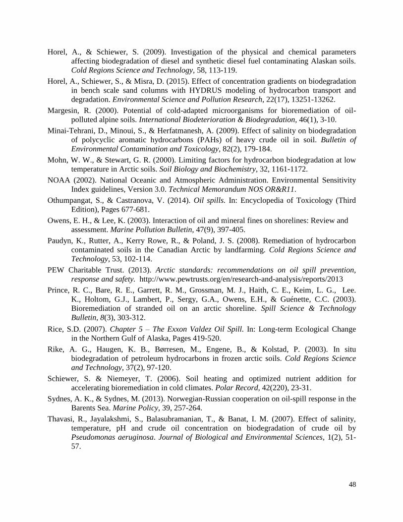
48

Horel, A., & Schiewer, S. (2009). Investigation of the physical and chemical parameters

affecting biodegradation of diesel and synthetic diesel fuel contaminating Alaskan soils.

Cold Regions Science and Technology, 58, 113-119.

Horel, A., Schiewer, S., & Misra, D. (2015). Effect of concentration gradients on biodegradation

in bench scale sand columns with HYDRUS modeling of hydrocarbon transport and

degradation. Environmental Science and Pollution Research, 22(17), 13251-13262.

Margesin, R. (2000). Potential of cold-adapted microorganisms for bioremediation of oil-

polluted alpine soils. International Biodeterioration & Biodegradation, 46(1), 3-10.

Minai-Tehrani, D., Minoui, S., & Herfatmanesh, A. (2009). Effect of salinity on biodegradation

of polycyclic aromatic hydrocarbons (PAHs) of heavy crude oil in soil. Bulletin of

Environmental Contamination and Toxicology, 82(2), 179-184.

Mohn, W. W., & Stewart, G. R. (2000). Limiting factors for hydrocarbon biodegradation at low

temperature in Arctic soils. Soil Biology and Biochemistry, 32, 1161-1172.

NOAA (2002). National Oceanic and Atmospheric Administration. Environmental Sensitivity

Index guidelines, Version 3.0. Technical Memorandum NOS OR&R11.

Othumpangat, S., & Castranova, V. (2014). Oil spills. In: Encyclopedia of Toxicology (Third

Edition), Pages 677-681.

Owens, E. H., & Lee, K. (2003). Interaction of oil and mineral fines on shorelines: Review and

assessment. Marine Pollution Bulletin, 47(9), 397-405.

Paudyn, K., Rutter, A., Kerry Rowe, R., & Poland, J. S. (2008). Remediation of hydrocarbon

contaminated soils in the Canadian Arctic by landfarming. Cold Regions Science and

Technology, 53, 102-114.

PEW Charitable Trust. (2013). Arctic standards: recommendations on oil spill prevention,

response and safety. http://www.pewtrusts.org/en/research-and-analysis/reports/2013

Prince, R. C., Bare, R. E., Garrett, R. M., Grossman, M. J., Haith, C. E., Keim, L. G., Lee.

K., Holtom, G.J., Lambert, P., Sergy, G.A., Owens, E.H., & Guénette, C.C. (2003).

Bioremediation of stranded oil on an arctic shoreline. Spill Science & Technology

Bulletin, 8(3), 303-312.

Rice, S.D. (2007). Chapter 5 – The Exxon Valdez Oil Spill. In: Long-term Ecological Change

in the Northern Gulf of Alaska, Pages 419-520.

Rike, A. G., Haugen, K. B., Børresen, M., Engene, B., & Kolstad, P. (2003). In situ

biodegradation of petroleum hydrocarbons in frozen arctic soils. Cold Regions Science

and Technology, 37(2), 97-120.

Schiewer, S. & Niemeyer, T. (2006). Soil heating and optimized nutrient addition for

accelerating bioremediation in cold climates. Polar Record, 42(220), 23-31.

Sydnes, A. K., & Sydnes, M. (2013). Norwegian-Russian cooperation on oil-spill response in the

Barents Sea. Marine Policy, 39, 257-264.

Thavasi, R., Jayalakshmi, S., Balasubramanian, T., & Banat, I. M. (2007). Effect of salinity,

temperature, pH and crude oil concentration on biodegradation of crude oil by

Pseudomonas aeruginosa. Journal of Biological and Environmental Sciences, 1(2), 51-

57.

49

Wrabel, M. L., & Peckol, P. (2000). Effects of bioremediation on toxicity and chemical

composition of no. 2 fuel oil: Growth responses of the brown alga Fucus vesiculosus.

Marine Pollution Bulletin, 40(2), 135-139.

Wrenn, B. A., & Venosa, A. D. (1996). Selective enumeration of aromatic and aliphatic

hydrocarbondegrading bacteria by a most-probable-number procedure. Canadian Journal

of Microbiology, 42(3), 252-258.

Yang, S. Z., Jin H. J., Wei Z., He R. X., Ji Y. J., Li X. M., & Yu S. P. (2009). Bioremediation of

oil spills in cold environments: A review. Pedosphere, 19(3), 371-381.

50

APPENDIX

MPN results

MPN results were obtained using the EPA MPN calculator after visual identification of positive

wells (Table A.1). As shown in Figure A.1, the data do not show a clear trend over time and do

not follow the growth kinetics anticipated from the review of prior studies.

The “sterile” microcosms contained similar quantities of hydrocarbon degraders as the other

microcosms. This means sterilization by autoclaving had no lasting effect. Either the autoclaving

was not effective in the first place, and/or microbes present in the ambient air colonized the

microcosms. The latter is quite likely since no biological hood was available for these

experiments. During daily CO2 measurements, microcosms had to be opened, which could have

allowed microbes to enter the sterile microcosms.

Figure A1. MPN of crude oil degraders from 20°C experiments.

Table A1. MPN values of number of microbes per gram (MPN/g) of soil at 20°C.

Days CoS1 con CoS1 ster C1S1 ster C1S1 exp C1S2 exp C2S1 exp C2S2 exp

14 0 370 11989 1053 466 9328 0

28 0 466 119893 734 119893 7344 360

42 0 105 7344 10532 1894 1913 310

51

A further potential error source was the difficulty of identifying the color change indicating

positive samples. Figure A.2 shows an MPN plate using crude oil as a carbon source at 20°C.

Due to the presence of a dark surface layer of crude oil, it was difficult to visually identify the

positive wells.

Therefore, diesel was used as a carbon source for 3°C study. An example of a well plate using

samples from 3°C experiments incubated at 10°C with diesel as a carbon source is shown in

Figure A.3. A temperature of 10°C was used to incubate well plates from the 3°C experimental

study because incubation at 3°C may not have resulted in color change within the incubation

period. However, even at 10°C, only one well developed a pink color (i.e., positive for diesel

degraders) which is not a good representative of the number of microbes in the sediments.

Therefore, no MPN can be reported for the 3°C experiments.

The absence of color change in wells could be due to the lower temperature where the microbes

would not yet degrade the diesel in the Bushnell medium since lag phases are typically longer at

low temperature (Horel 2011). It is likely that microbes were inactive during the incubation

period, because after their incubation at low temperature, these plates were moved to a hazardous

waste cabinet at room temperature, where all wells changed to a pink color within a few days.

This shows that microbes must have been present, and those microbes became active after being

discarded, consumed the diesel, and caused a color change. Therefore, no data are available for

3°C. For future studies, it is recommended to change the protocol, possibly by using longer

incubation periods or higher incubation temperatures, to ensure that microbes become active

during incubation.

Figure A2. MPN plate for the C1S2 and C2S1 samples at 20°C with crude oil as C source.

52

Figure A3. MPN plate for C2S1 and C2S2 samples at 3°C with diesel as C source.

Wave tank photographs

Figures A4-A8 show the wave tank experiment.

Figure A4. Addition of pebble sediment

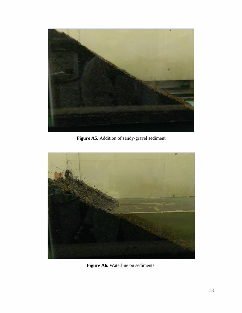
53

Figure A5. Addition of sandy-gravel sediment

Figure A6. Waterline on sediments.

54

Figure A7. Wave tank in action.

Figure A8. Sequence of steps in wave tank experiment (a) Sediment before water addition, (b)

sediment with water, and (c) sediment with water and crude oil.

a b c

The Department of the Interior Mission As the Nation’s principal conservation agency, the Department of the Interior has responsibility for most of our nationally owned public lands and natural resources. This includes fostering the sound use of our land and water resources, protecting our fish, wildlife and biological diversity; preserving the environmental and cultural values of our national parks and historical places; and providing for the enjoyment of life through outdoor recreation. The Department assesses our energy and mineral resources and works to ensure that their development is in the best interests of all our people by encouraging stewardship and citizen participation in their care. The Department also has a major responsibility for American Indian reservation communities and for people who live in island communities.

The Bureau of Ocean Energy Management The Bureau of Ocean Energy Management (BOEM) works to manage the exploration and development of the nation's offshore resources in a way that appropriately balances economic development, energy independence, and environmental protection through oil and gas leases, renewable energy development and environmental reviews and studies.