Biochar and activated carbon filters for greywater...

Examensarbete 2012:14 ISSN 1654-9392 Uppsala 2012

Photo: Christina Berger

Biochar and activated carbon filters for greywater treatment – comparison of organic matter and nutrients removal Christina Berger

SLU, Sveriges lantbruksuniversitet SUAS, Swedish University of Agricultural Sciences Institutionen för energi och teknik Department of Energy and technology Swedish title: Filter av biokol och aktivt kol för behandling av BDT-vatten – jämförelse av reduktionen av organiskt material och näringsämnen English title: Biochar and activated carbon filters for greywater treatment – comparison of organic matter and nutrients removal Author: Christina Berger Supervisor: Sahar Dalahmeh External Co-Supervisor: Günter Langergraber Examiner: Håkan Jönsson Credits: 30 hec Level: Advanced, A2E Course title: Independent Project in Environmental Science Course code: EX0431 Programme/education: Master thesis in EnvEURO Place of publication: Uppsala, Sweden Year of publication: 2012 Title of series: Examensarbete/Thesis no: 2012:14 ISSN 1654-9392 Cover Photo: Christina Berger Keywords: Phosphorous removal, nitrogen removal, vertical flow, anionic

2

Abstract

Activated carbon has long been used for the treatment of water. The industrial activation processes increase the environmental footprint and cost of this product. Biochar, which is organic material pyrolyzed/charred, often by means of simple and low cost techniques, might be an interesting alternative to replace the industrial activated carbon for greywater cleaning. The objective of this study is to evaluate and compare biochar and activated carbon by assessing reductions of COD, MBAS, Tot-N and Tot-P as well as the transformation of nitrogen in the greywater-infiltrated filters. The activated carbon and biochar were packed to a depth of 50 cm into columns with a diameter of 4.3 cm. The columns were fed with artificial greywater at a hydraulic loading rate of 0.043 m3/m2/day under vertical flow. The bulk density, particle density, total porosity and residence time of the filters were initially measured. Then their water cleaning capacity was assessed over a period of ten weeks based on nine chemical parameters (pH, EC, NH4-N, NO3-N, Tot-N, PO4-P, Tot-P, MBAS and COD). The residence time in the activated carbon filters was 119 hours and in the biochar filters 108 hours. Both materials cleaned the greywater well from organic matter, with 99% efficiency for COD and MBAS. It is remarkable that biochar removed Tot-P and PO4 –P more effectively than activated carbon, on average to 89% in case of Tot-P and 86% in case of PO4 –P. The efficiency of biochar in Tot-N and NH4-N was not stable, whereas activated carbon had stable efficiency levels of 97% and 98% for Tot-N and NH4–N. Further investigations are recommended in regards to how long the cleaning capacity of biochar lasts and how the performance of the filter changes under an increased load of greywater. The performance of biochar from different parent materials and recycling options for the used filter materials are also interesting aspects for future research.

3

Foreword

This Master Thesis work has been conducted at the Department of Energy and Technology at the Swedish University of Agricultural Sciences (Sveriges Landbruksuniversitet, SLU), in Uppsala. It was financed by the Swedish Research Council FORMAS and the Swedish International Development Cooperation Agency, Sida. The work was conducted as part of a research project that focused on on-site treatment of greywater in order to upgrade it to a resource for irrigation, service or recharge. I would like to thank my supervisor, Sahar Dalahmeh (Department of Energy and Technology/SLU), for her continuous supervision during the planning of the study, laboratory work, data analysis and writing process. Furthermore I wish to thank my second supervisor, Günter Langergraber (Department of Water, Atmosphere and Environment/ University of Applied Life Sciences in Vienna), for professional feedback and supervision meetings. I also want to thank Håkan Jönsson (Department of Energy and Technology/SLU) for offering his time and scholarly advice. On a related note I need to express my appreciation for Lars Hylander from Uppsala University and the local biochar group for providing the biochar and helpful information and meetings concerning the biochar material. I also extend my gratitude to Tomas Thierfelder for helping me with the statistical tests and to Nilima Rabl for linguistic advice.

4

Contents

Abstract

Foreword

Contents ..................................................................................................................... 4

Introduction ................................................................................................................ 5

Material and Methods ................................................................................................ 8 Experimental Plan................................................................................................................... 8 Characteristics of Filter Materials .......................................................................................... 9 Buildup of Filters .................................................................................................................... 9 Determination of Physical Parameters ................................................................................. 10 Residence Time .................................................................................................................... 12 Greywater Preparation and Composition ............................................................................. 12 Feeding of the Filters ............................................................................................................ 13 Sampling and Chemical Analysis ......................................................................................... 14 Statistics ................................................................................................................................ 17

Results ...................................................................................................................... 19 Particle Density, Bulk Density, Total Porosity and Residence Time ................................... 19 Statistical tests ...................................................................................................................... 21 Pollutants Concentrations and Treatment Efficiency: Overview ......................................... 22 Performance of Biochar and Activated Carbon Filters ........................................................ 24

Discussion ................................................................................................................ 34 Influence of Physical Parameters on Filter Performance ..................................................... 34 Greywater Influent Characteristics ....................................................................................... 34 Organic Matter Removal ...................................................................................................... 35 Phosphorous Removal .......................................................................................................... 35 Nitrogen Removal................................................................................................................. 35

Conclusion ............................................................................................................... 37

References ............................................................................................................... 38

Appendices .............................................................................................................. 40

5

Introduction

Greywater is household wastewater in all its aspects - including water from bathtubs, showers and hand basins to kitchen sinks and laundry machines - with the exception that it does not contain any water derived from the toilet (Eriksson et al., 2002). It accounts for approximately 50-80% of a household’s total wastewater (Li et al., 2009). The main target in greywater treatment is the reduction of easily degradable organic compounds responsible for bad odors (Ridderstolpe, 2004) and the immediate processing and reuse of greywater before anaerobic conditions occur (Al-Jayyousi 2003). The release of untreated greywater to the environment can lead to oxygen depletion and increased turbidity in the receiving water body (Morel & Diener, 2006). The reduction of organic matter in treated greywater, including surfactants, was measured in this study. Furthermore, nutrient reduction was monitored. Levels of nutrients in greywater are low if compared to normal wastewater that contains toilet water. In untreated greywater - with phosphorous and nitrogen levels below the concentrations normally found in water used for fertilization - no negative effects on soils were detected upon direct irrigation reuse (Gross et al., 2005). However, nutrients from untreated greywater disposed into the environment can lead to eutrophication (Morel & Diener, 2006). Untreated greywater compared to treated wastewater contains a much lower density of pathogens; the reduction of pathogens was not investigated in this study, but is still a secondary target in greywater treatment (Ridderstolpe, 2004) and topic of current research. Hydraulic load and pollution load of greywater depend on household activities and are crucial for the design of an appropriate greywater treatment system (Ridderstolpe, 2004). Organic matter levels (expressed as chemical oxygen demand, COD) in greywater range between a COD of 13 and 8000 mg/l and are expected to be almost similar to household wastewater -which includes the waste from toilet facilities- simply because the source of COD in mixed wastewater also consists mainly of chemicals such as dishwashing or laundry detergent (Eriksson et al., 2002). The COD level depends on the use of such products and also on the water consumption of the household. Greywater studies conducted in rural villages of Jordan, for instance with greywater consumption of 14 liters /capita/day reported COD 2568 mg/l (Halalsheh et al., 2008) whereas studies from a community in Sweden with greywater consumption of around 66 liters/capita/day reported COD 588 mg/l (Palmquist & Hanæus, 2005). Total nitrogen levels in greywater are ranging from 0.6 to 74 mg/l in literature reviewed by Eriksson et al. (2002), which is very low if compared to household wastewater, due to the fact that urine, the main source of nitrogen in wastewater, is not included in the greywater. Total phosphorous levels in greywater depend primarily on whether a country has banned the use of phosphorous containing detergents. Levels are ranging from 4 to 14 mg/l where non-phosphorous detergents are used and from 6 to 23 mg/l where detergents still contain phosphorous (Eriksson et al., 2002). Through reusing the treated greywater for irrigation, toilet flushing, outdoor applications, development and preservation of wetlands or into-ground infiltration (Eriksson et al., 2002),a community can benefit by saving water and protecting the environment. Reasons for reusing greywater can be water shortage (e.g. Australia), large demands of freshwater (e.g. Japan) or economical considerations (Eriksson et al., 2002). In rural and peri-urban areas of low and middle-income countries, untreated greywater is commonly used for agriculture or discharged into drainage channels, open fields or natural aquatic systems (Morel & Diener, 2006). In these situations, outbreaks of waterborne diseases are of concern for public health, and bad odors as well as aesthetic deterioration may determine living conditions (Morel & Diener, 2006). Faced with stress placed on water resources as well as increased development and

6

environmental protection goals, some countries are already giving special attention to the reuse of treated wastewater, as for instance the arid countries of the Middle East and North Africa (Smith & Bani-Melhem, 2012). In order to contribute to the protection of public health and environment, greywater treatment/ management should achieve a number of basic requirements: ensurance of soil fertility, socio-cultural and economic acceptance, compliance with regulations and standards, as well as the provision of simple and user friendly guidance (Morel & Diener, 2006). Greywater management consists of the following elements: source control, plumbing and pipe system, pre-treatment, treatment, and discharge or reuse (Ridderstolpe, 2004). The purpose of pre-treatment or primary treatment is to remove coarse solids, settleable suspended solids, oil, grease and part of the organic matter (Morel & Diener 2006) through screening or settling, for instance using a septic tank system. Greywater treatment aims at reducing dissolved and remaining suspended organic matter, pathogens and nutrients in the greywater (Morel & Diener 2006). Li et al. (2009) reviewed and evaluated literature of different greywater treatment alternatives published between 1995 and 2008 and brought up a reuse scheme according to greywater characteristics. They make recommendations to follow up on pre-treatment: low strength greywater should undergo chemical treatment with subsequent membrane or sand filtration, while medium and high strength greywater demands aerobic biological treatment (Rotating biological contactor, sequencing batch reactor, and constructed wetland) with subsequent sand or membrane filtration. They consider aerobic biological processes with physical filtration and, eventually, disinfection as the most economical and feasible solution for greywater recycling. Ridderstolpe (2004) also recommends the use of aerobic attached biofilm techniques in greywater treatment that leads to biological degradation of organic matter under aerobic conditions. Vertical-flow filter systems are often implemented in constructed wetlands. To ensure oxygen supply, the greywater is intermittently and evenly spread over the filter surface typically made from sand and gravel, and aerobic attached biofilm processes develop (Morel & Diener 2006). These filter materials, which are commonly used as growing medium, are of mineral origin (Runying et al. 2009). Other mineral substances, such as slag or charcoal, can increase phosphorous removal due to high adsorption capacity (Runying et al.). In previous lab experiments Dalahmeh et al. (2012) tested appropriate materials for small-scale greywater vertical filters: The goals of these experiments were to analyze and compare the reduction in BOD5, COD, MBAS, phosphorous and certain microorganisms for artificial greywater (Dalahmeh et al. 2012). Activated carbon showed superior performance in reducing organics (94% COD & 97% BOD reduction), surfactants (99% reduction), and total phosphorous (91% reduction). Activated carbon also reduced total nitrogen by 98% (Dalahmeh at al. 2012). The activation of the carbon is expensive and has thus prevented its use in waste water treatment (Streubel, 2011). Charcoal or biochar is produced from different organic materials in a rather similar way as activated carbon, but without the activation. It is therefore interesting for field application, where it could function as an alternative to activated carbon. Activated carbon can be produced either from a biochar-type substance or coal by different possible processes (e.g steam or chemicals), increasing its surface area for use in industrial processes such as filtration (Lehmann & Joseph, 2009). Granular activated carbon (GAC) filters have been used for a long time to adsorb different organic macropolutants, disinfectant by-products, as well as odour and taste compounds from water (Velten, 2008). Biochar and charcoal are basically the same: organic parent material being charred/ pyrolized without the presence of sufficient oxygen. The term “biochar” is used when the material is charred with

7

the intention of amending it to soils, using it as carbon sink or filtration of percolating soil water, whereas the term “charcoal” is mainly used when intended to be applied as a source of energy (Lehmann & Joseph, 2009). The first evidence of biochar use in history goes back to the Amazonia dark earth “terra preta” that formed as a result of indigenous settlement in Brazil (Steiner, 2007). Research has documented positive effects of biochar amendment to soil on the vegetation growth for quite some time, but its development for environmental management on a global scale is quite recent (Lehmann & Joseph, 2009). The international biochar initiative reports 40 biochar groups worldwide (IBI, 2012). The objectives of the biochar application for environmental management are soil improvement, waste management, climate change mitigation and energy production (Lehmann & Joseph, 2009). Animal and crop wastes from agriculture can have negative effects on the environment due to pollution of ground and surface waters (Carpenter et al. 1998). On the other hand, there are advantages (e.g. removal of organic pollutants from wastewater) when using organic by-products such as bark, compost, wheat straw and wood chips as filter material (Dalahmeh et al. 2011). Agricultural wastes and other by-products can be used as a resource for pyrolysis, resulting in biochar (Lehmann & Joseph, 2009). By noting that organic wastes can have beneficial properties instead of merely functioning as pollutants, they can serve new ideas for environmental management, such as the use of biochar in form of charred agricultural residues as filter materials for greywater. The overall goal of this thesis is to study the use of biochar as a replacement/ alternative for activated carbon to serve as a filter material for greywater purification. The specific objectives are (i) to evaluate the COD, MBAS, Tot-N and Tot-P reductions in greywater infiltrated filters made of biochar and activated carbon and (ii) to compare the greywater purification efficiency of biochar and activated carbon.

Mater

Experim

Figure 1 A columbiochar greywatfractionFigure 1applicat

1. Mdw

2. Tud

rial and

mental Pla

1. Experime

mn experimeand activat

ter. The six s of the mai

1).The phystion phase a

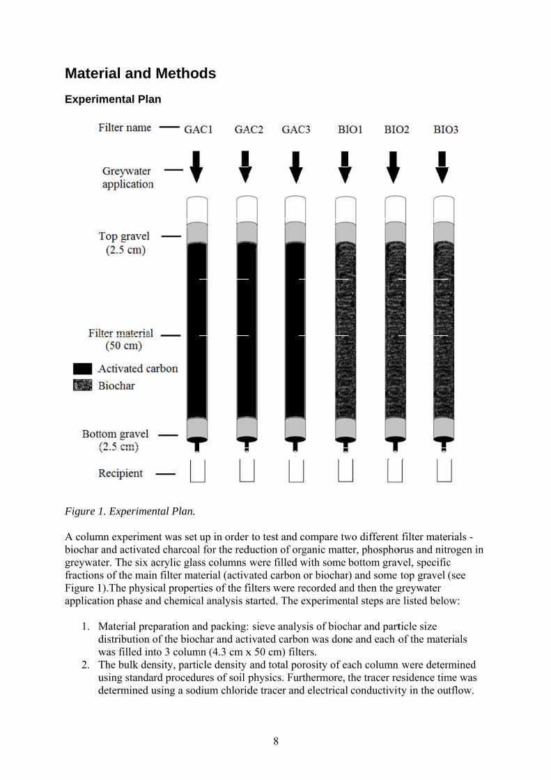
Material predistributionwas filled inThe bulk deusing standadetermined

d Metho

an

ental Plan.

ent was set ted charcoalacrylic glasin filter mat

sical propertand chemica

eparation ann of the biocnto 3 columensity, partiard proceduusing a sod

ds

up in order l for the redss columns terial (activties of the fial analysis s

nd packing:char and actimn (4.3 cm x

cle density ures of soil pdium chlorid

8

to test and duction of orwere filled

vated carbonfilters were rstarted. The

sieve analyivated carbo

x 50 cm) filtand total pophysics. Fude tracer an

compare twrganic mattewith some b

n or biocharrecorded anexperiment

ysis of biochon was donters. orosity of earthermore, t

nd electrical

wo different er, phosphobottom grav) and some

nd then the gtal steps are

har and parte and each o

ach column the tracer reconductivit

t filter materorus and nitrvel, specifictop gravel

greywater e listed belo

ticle size of the mate

n were deteresidence timty in the ou

rials -rogen in c (see

ow:

rials

mined me was tflow.

9

3. Over a period of 10 weeks from Monday until Friday artificial greywater - 42 ml at 9 a.m. and 21 ml at 4 p.m. - was distributed over the filters, corresponding to a load of 0.043 m³/m²/day.

4. The effluent greywater from the activated carbon and biochar filters was sampled twice a week from week 1 to 5 and once a week from week 6 to 10. It was tested for pH, electrical conductivity (EC), chemical oxygen demand (COD), methylene blue active substances (MBAS) as indicator for anionic surfactants, nitrate (NO3-N), ammonium (NH4-N), total nitrogen (Tot-N), phosphate (PO4-P) and total phosphorous (Tot-P).

Characteristics of Filter Materials

Activated carbon was bought from Merck with particle size 1.5 mm (granular) and 3-5 mm long activated carbon pellets with a diameter inbetween 0.85 and 1.7 mm (10-18 mesh). The activated carbon originated from black coal. The specific surface area of both carbon fractions was >1000 m2 g-1 and the effective size was 1.4 mm. The biochar originated from chopped salix, a broadleaf tree with low density. It was grown in Germany and charred at a temperature of 450°C. In order to have particle sizes that were comparable to the activated carbon and also comparable to previous greywater studies by Dalahmeh et al (2012), biochar was sieved on a stack of sieves with mesh openings of 1 mm, 1.4 mm, 2.8 mm and 5 mm placed on the mechanical shaker (Retsch, Haan, Germany). The uppermost sieve was loaded with four cups (around 170 g) of pre-sieved biochar material. The shaker was run at 30 rpm for ten minutes and finally the fractions 1-1.4 mm and 2.8-5 mm were selected to be packed in the cylinders. Pictures of the different fractions of the biochar are shown in Appendix 1. Of the raw biochar, 41% consisted of particles smaller than 1mm (see Table 1) and were mainly removed manually before the mechanical shaking. Table 1. Particle size distribution of the biochar before sieving Particle size (mm) Percentage (%) <1 41 1-1.4 7 1.4-2.8 20 >5 13

Buildup of Filters

Six acrylic glass cylinders, three for each of the activated carbon and biochar materials, were used as filter columns. The cylinders were 65 cm long and had a diameter of 4.3 cm. The bottom of each column was sealed by a round plastic plate with a small 0.5 cm diameter outlet. For biochar, two parts by weight of particle size 1-1.4 mm and three parts by weight of particles size 2.8-5 mm were mixed in a bucket. For activated carbon, two parts by weight of particle size 1.5 mm and three parts by weight of particle size 3-5 mm were mixed. The content for each filter was homogenously mixed in the bucket with a spoon. These specific ratios were chosen in order to obtain a similar effective size and uniformity coefficient as sand filters and to design them comparable to the filters used in Dalahmeh et al. (2012). As illustrated in Figure 1, the columns were filled up to 2.5 cm with bottom gravel (0.5 cm diameter), then 50 cm of the filter material evenly mixed in the bucket were added to the column spoon by spoon in order to pack them as densely as possible. For the same reason, the outside of the column was knocked after each spoon. A layer of 2.5 cm top gravel was added and finally the whole column was packed into aluminum foil in order to prevent light

10

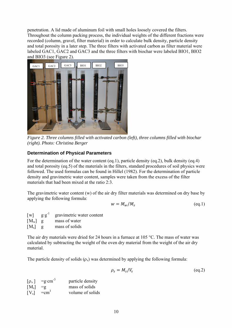
penetration. A lid made of aluminum foil with small holes loosely covered the filters. Throughout the column packing process, the individual weights of the different fractions were recorded (column, gravel, filter material) in order to calculate bulk density, particle density and total porosity in a later step. The three filters with activated carbon as filter material were labeled GAC1, GAC2 and GAC3 and the three filters with biochar were labeled BIO1, BIO2 and BIO3 (see Figure 2).

Figure 2. Three columns filled with activated carbon (left), three columns filled with biochar (right). Photo: Christina Berger

Determination of Physical Parameters

For the determination of the water content (eq.1), particle density (eq.2), bulk density (eq.4) and total porosity (eq.5) of the materials in the filters, standard procedures of soil physics were followed. The used formulas can be found in Hillel (1982). For the determination of particle density and gravimetric water content, samples were taken from the excess of the filter materials that had been mixed at the ratio 2:3. The gravimetric water content (w) of the air dry filter materials was determined on dry base by applying the following formula:

/ (eq.1)

w g·g-1 gravimetric water content Mw g mass of water Ms g mass of solids The air dry materials were dried for 24 hours in a furnace at 105 °C. The mass of water was calculated by subtracting the weight of the oven dry material from the weight of the air dry material. The particle density of solids (s) was determined by applying the following formula:

/ (eq.2) s =g·cm-3 particle density Ms =g mass of solids Vs =cm3 volume of solids

GAC1 GAC2 GAC3 BIO1 BIO2 BIO3

11

Two volumetric flasks were filled up to a third with the oven dried materials, one with biochar, the other one with granular activated carbon. The flasks were filled with deionized water that had settled for three days until up to the half. Then the flasks were placed for boiling on a hot plate for around 10 minutes, until no more air bubbles came up. The cooled and covered flasks remained standing in the lab for 24 hours and then they were filled up with deionized water to the volume line. The weight of the flasks was recorded for all steps and at the end also the temperature of the water in the flask was recorded. The determination of the density of the water at the measured temperature was done with the help of the following formula according to Tanaka et al. (2011):

∙ 1 ∙

∙ (eq.3)

w (t) = kg·m-3 density of clean water, free from air, having the isotopic

composition of SMOW (Standard Mean Ocean Water) at p0=101325 Pa

t = ˚C temperature a1 = ˚C coefficient(-3.983035) a2 = ˚C coefficient (301.797) a3 = ˚C coefficient (522528.9) a4 = ˚C coefficient (69.34881) a5 = kg·m-3 coefficient (999.974950) The density of the water at the measured temperature was also compared with a water density table for pure water (Simetric, 2012) showing very similar density values. The water denisty was multiplied by the mass of water in order to obtain the volume of water. By abstracting the volume of water from the total volume, the volume of solids was calculated. The mass of solids was then divided by the volume of solids to obtain particle density (see eq. 2). The bulk density (b) was determined applying the following formula:

/ (eq.4)

b = g·cm-3 bulk density Ms = g mass of solids Vt = cm3 total volume of the representative soil (here: carbon) body Vs = cm3 volume of solids Va = cm3 volume of air Vw = cm3 volume of water The total volume (Vt) in our case is the part of the column that is filled with the filter material (excluding top and bottom gravel). The column was filled with 50 cm of filter material and had a diameter of 4.3 cm. The mass of solids was determined by subtracting the mass of water from the air dry filter material in the column. The mass of water was calculated by multiplying the airdry weight of the filter material by the gravimetric water content.

12

The total porosity was calculated with the formula:

1 (eq.5)

f = cm3· cm-3 Porosity b = g·cm-3 bulk density s =g·cm-3 particle density

Residence Time

Initially the filters were fed with distilled water (42 ml at 9 a.m. and 21 ml at 4 p.m.). A pulse of 42 ml of a 1% sodium chloride solution was added as a tracer for residence time measurements and subsequently the electrical conductivity (EC) of the outflow from the filters was measured as a function of time. The EC of the outflow water was measured using a Conductivity Pocket Meter (WTW, Germany). Initially, before starting the tracer experiment, the effluent from the filters had an EC of 129.9 μS/cm (activated carbon) and 1188.5 μS/cm (biochar). The increase and decrease in EC (“Net EC”) over fifteen days was plotted by subtracting these background values. Each time the EC in the effluent was measured, the respective outflow volume was recorded. The recorded effluent volume was multiplied by the measured EC and cumulated over time. The total EC of the tracer added to each filter was 776.2 mS*ml/cm being the volume of the pulse (42ml) times the EC of the sodium chloride solution (18.48 mS/cm). The residence time of the tracer within one material was calculated as the mean of the cumulated EC values of the three filters of one filter material divided by 776.2 mS/cm and then plotted. The time it took to recover 50% of the tracer was reported as mean residence time.

Greywater Preparation and Composition

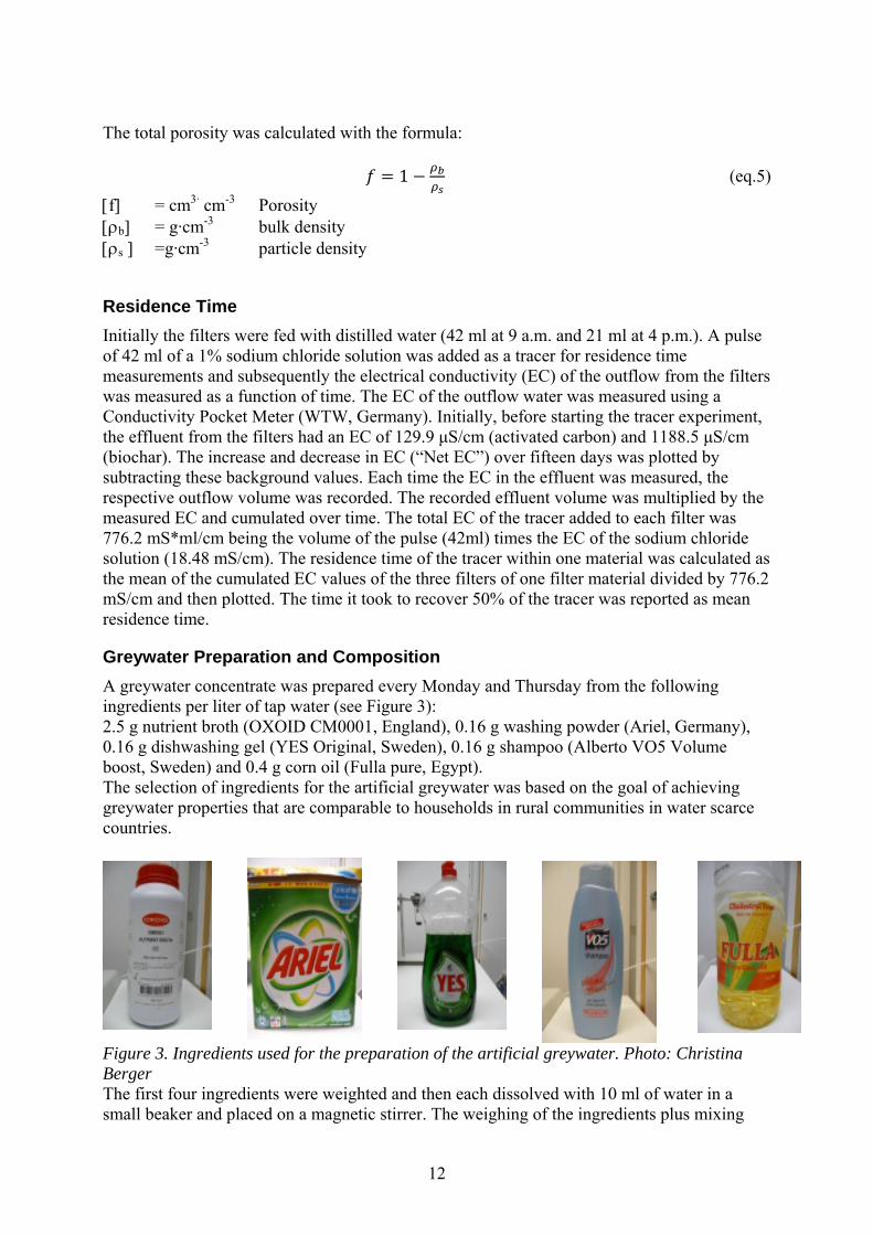
A greywater concentrate was prepared every Monday and Thursday from the following ingredients per liter of tap water (see Figure 3): 2.5 g nutrient broth (OXOID CM0001, England), 0.16 g washing powder (Ariel, Germany), 0.16 g dishwashing gel (YES Original, Sweden), 0.16 g shampoo (Alberto VO5 Volume boost, Sweden) and 0.4 g corn oil (Fulla pure, Egypt). The selection of ingredients for the artificial greywater was based on the goal of achieving greywater properties that are comparable to households in rural communities in water scarce countries.

Figure 3. Ingredients used for the preparation of the artificial greywater. Photo: Christina Berger The first four ingredients were weighted and then each dissolved with 10 ml of water in a small beaker and placed on a magnetic stirrer. The weighing of the ingredients plus mixing

13

with water took around 4 minutes per ingredient and as one beaker was ready it was placed for stirring on the magnetic stirrer and remained there until the final mixing (ranging from 8 to 16 minutes depending on the ingredient). The ingredients were always dissolved one after the other in the above listed order. This order was chosen because the first two ingredients being in powder form needed more time to dissolve. The corn oil and 10 ml of water were put directly into a big beaker in order to prevent oil losses. Then 950 ml of hot tap water (temperature ranging from 40-43 °C) were used to rinse the small beakers with the dissolved ingredients into the big beaker. The mix of all the ingredients and the one liter of water (50 ml+ 950 ml) were placed on the magnetic stirrer for another 10 minutes. 250 ml of this basic concentrate were used immediately for further mixing (see next step) and the rest was stored in a bottle in the fridge at 8°C. The obtained concentrate was the double of the needed concentration for the feeding of the filters. As a feeding temperature of 25°C was targeted, the right temperature of the final greywater could be adjusted by adding either hot or cold tap water depending on the temperature of the greywater concentrate. On Monday and Thursday morning the concentrate used for dilution was freshly prepared and had a temperature of around 37°C. Therefore it was mixed at the ratio 1:1 with cold tap water (15-20°C), resulting in a feeding temperature between 26 and 28°C. For all the other feeding events the greywater concentrate came out of the fridge and after a mixing of the bottle for five minutes, the concentrate temperature was around 10°C. The needed amount of greywater concentrate was taken from the bottle and the bottle with the remaining concentrate was again stored in the fridge. In this case the final greywater was obtained by mixing the concentrate at the ratio 1:1 with hot tap water (40-43°C), resulting in a feeding temperature between 23 and 26°C.

Feeding of the Filters

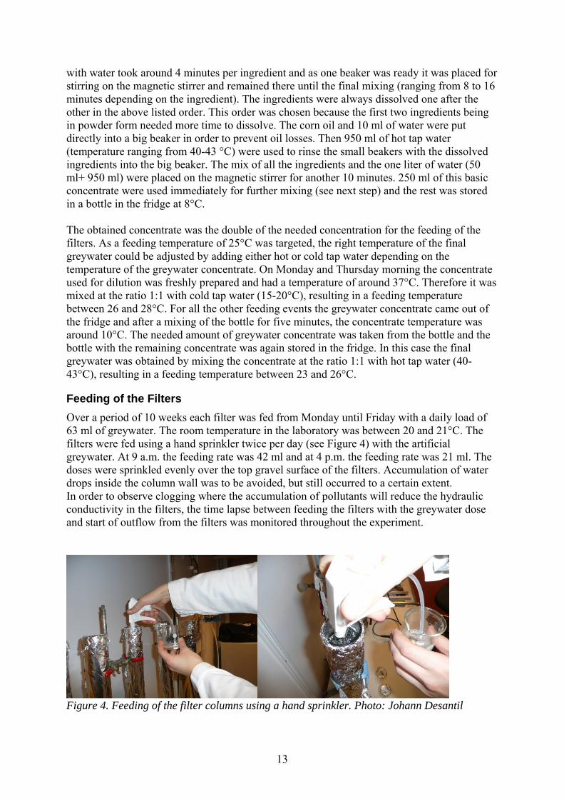
Over a period of 10 weeks each filter was fed from Monday until Friday with a daily load of 63 ml of greywater. The room temperature in the laboratory was between 20 and 21°C. The filters were fed using a hand sprinkler twice per day (see Figure 4) with the artificial greywater. At 9 a.m. the feeding rate was 42 ml and at 4 p.m. the feeding rate was 21 ml. The doses were sprinkled evenly over the top gravel surface of the filters. Accumulation of water drops inside the column wall was to be avoided, but still occurred to a certain extent. In order to observe clogging where the accumulation of pollutants will reduce the hydraulic conductivity in the filters, the time lapse between feeding the filters with the greywater dose and start of outflow from the filters was monitored throughout the experiment.

Figure 4. Feeding of the filter columns using a hand sprinkler. Photo: Johann Desantil

14

Sampling and Chemical Analysis

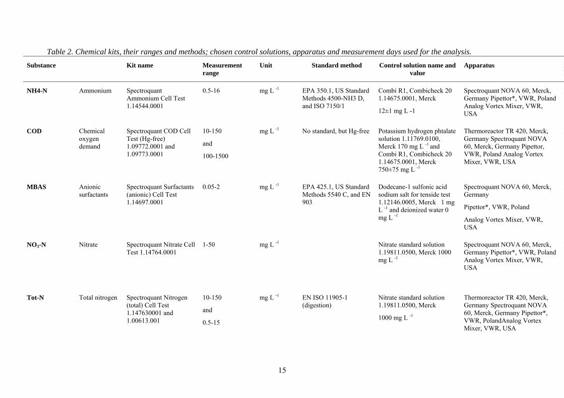
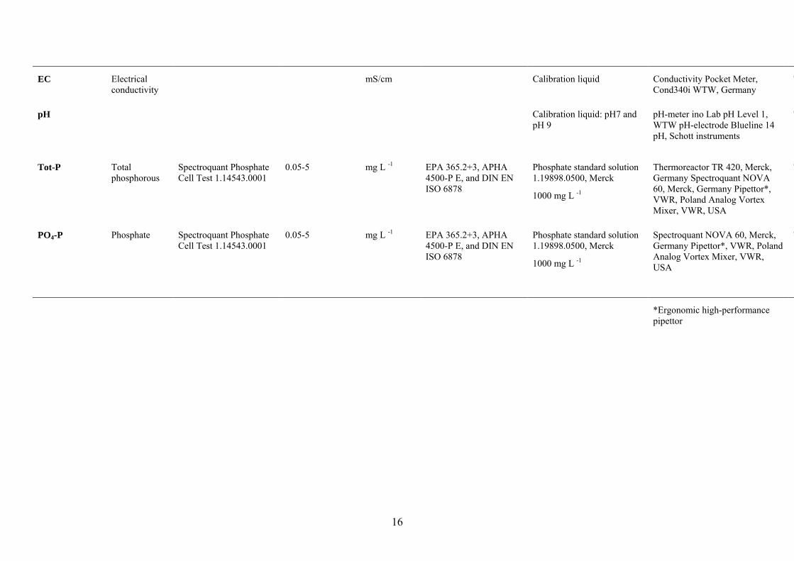
Samples of the inflow and outflow were collected for the chemical analysis. Samples of the inflow greywater were taken at the time of feeding and stored in the fridge in order to be analyzed after the feeding event together with the outflow samples. During the first five weeks of the experiment, the following chemical parameters were determined twice a week; NH4-N, COD, MBAS, NO3-N and Tot-N on Monday and Thursday and EC, pH, PO4-P and Tot-P on Tuesday and Friday. During the last 5 weeks of the experiment, the samples were collected and analyzed once a week; NH4-N, COD, MBAS, NO3-N and Tot-N on Thursday and EC, pH, PO4-P and Tot-P on Friday as shown in Table 2. Outflow samples were taken immediately after enough water had accumulated in the outlet recipient. The parameters were determined using chemical kits and according to methods shown in Table 2. The procedures for the determination of each of the parameters were described in the manuals provided by the supplier and are attached in Appendix 2. The analytical quality was insured by using control solutions with known concentrations of the substance for every measurement series (specified in Table 2). For the EC determination, adjustment due to temperature deviation was needed. Nonlinear temperature compensation was selected on the EC meter and therefore EC values were already temperature adjusted. The pH meter had an integrated thermometer and pH values were also temperature adjusted automatically. The sampling size per parameter and measurement day was 16 for biochar and activated carbon together (2 replicates for each of the 6 filter effluents, 3 replicates for the inflow and 1 control solution), except pH and EC were measured without replicates due to the small amount of liquid available in the effluent. The total sampling size of effluent samples per filter material over the 65 days of the experiment was 42 for pH and EC, 66 for Mbas and 84 for COD, Tot-P, PO4-P, Tot-N, NH4-N and NO3-N.

15

Table 2. Chemical kits, their ranges and methods; chosen control solutions, apparatus and measurement days used for the analysis.

Substance Kit name Measurement range

Unit Standard method Control solution name and value

Apparatus DD

NH4-N Ammonium Spectroquant Ammonium Cell Test 1.14544.0001

0.5-16 mg L -1 EPA 350.1, US Standard Methods 4500-NH3 D, and ISO 7150/1

Combi R1, Combicheck 20 1.14675.0001, Merck

12±1 mg L -1

Spectroquant NOVA 60, Merck, Germany Pipettor*, VWR, Poland Analog Vortex Mixer, VWR, USA

M

COD Chemical oxygen demand

Spectroquant COD Cell Test (Hg-free) 1.09772.0001 and 1.09773.0001

10-150

and

100-1500

mg L -1 No standard, but Hg-free Potassium hydrogen phtalate solution 1.11769.0100, Merck 170 mg L -1 and Combi R1, Combicheck 20 1.14675.0001, Merck 750±75 mg L -1

Thermoreactor TR 420, Merck, Germany Spectroquant NOVA 60, Merck, Germany Pipettor, VWR, Poland Analog Vortex Mixer, VWR, USA

M

MBAS Anionic surfactants

Spectroquant Surfactants (anionic) Cell Test 1.14697.0001

0.05-2 mg L -1 EPA 425.1, US Standard Methods 5540 C, and EN 903

Dodecane-1 sulfonic acid sodium salt for tenside test 1.12146.0005, Merck 1 mg L -1 and deionized water 0 mg L -1

Spectroquant NOVA 60, Merck, Germany

Pipettor*, VWR, Poland

Analog Vortex Mixer, VWR, USA

M

NO3-N Nitrate Spectroquant Nitrate Cell Test 1.14764.0001

1-50 mg L -1 Nitrate standard solution 1.19811.0500, Merck 1000 mg L -1


M

Tot-N Total nitrogen Spectroquant Nitrogen (total) Cell Test 1.147630001 and 1.00613.001

10-150

and

0.5-15

mg L -1 EN ISO 11905-1 (digestion)

Nitrate standard solution 1.19811.0500, Merck

1000 mg L -1

Thermoreactor TR 420, Merck, Germany Spectroquant NOVA 60, Merck, Germany Pipettor*, VWR, PolandAnalog Vortex Mixer, VWR, USA

M

16

EC Electrical conductivity

mS/cm Calibration liquid Conductivity Pocket Meter, Cond340i WTW, Germany

T

pH Calibration liquid: pH7 and pH 9

pH-meter ino Lab pH Level 1, WTW pH-electrode Blueline 14 pH, Schott instruments

T

Tot-P Total phosphorous

Spectroquant Phosphate Cell Test 1.14543.0001

0.05-5 mg L -1 EPA 365.2+3, APHA 4500-P E, and DIN EN ISO 6878

Phosphate standard solution 1.19898.0500, Merck

1000 mg L -1

Thermoreactor TR 420, Merck, Germany Spectroquant NOVA 60, Merck, Germany Pipettor*, VWR, Poland Analog Vortex Mixer, VWR, USA

T

PO4-P Phosphate Spectroquant Phosphate Cell Test 1.14543.0001

0.05-5 mg L -1 EPA 365.2+3, APHA 4500-P E, and DIN EN ISO 6878

Phosphate standard solution 1.19898.0500, Merck

1000 mg L -1


T

*Ergonomic high-performance pipettor

17

The efficiency in reduction of the measured substances was calculated with the following formula:

(eq.7)

[E] Efficiency [Cin] Influent concentration (mg L-1) [Cout] Effluent concentration (mg L-1)

Statistics

The statistical program used to analyze the results is Statistica (Statsoft), version 10. The variables of one substance within one measuring day were organized according to the scheme shown in Table 3. Table 3. Organization of variables for statistical analysis

Date Week Day Column Repl-icate

Repl. ID

Week day Material Sub-stance

Concen-tration

Effi-ciency

In-flow

Cont

15.12.2011 50 64 1 1 163 Thursday GAC COD 10 0,99 1410 220

15.12.2011 50 64 1 2 163 Thursday GAC COD 11 0,99 1328

15.12.2011 50 64 2 1 164 Thursday GAC COD 10 0,99 1274

15.12.2011 50 64 2 2 164 Thursday GAC COD 10 0,99

15.12.2011 50 64 3 1 165 Thursday GAC COD 10 0,99

15.12.2011 50 64 3 2 165 Thursday GAC COD 14 0,99

15.12.2011 50 64 4 1 166 Thursday BIO COD 10 0,99

15.12.2011 50 64 4 2 166 Thursday BIO COD 11 0,99

15.12.2011 50 64 5 1 167 Thursday BIO COD 10 0,99

15.12.2011 50 64 5 2 167 Thursday BIO COD 10 0,99

15.12.2011 50 64 6 1 168 Thursday BIO COD 10 0,99

15.12.2011 50 64 6 2 168 Thursday BIO COD 18 0,99

As duplicate samples were taken for chemical analysis and each column also can be assumed to behave in its own way, independent observations cannot be assumed. On the contrary, covariance can be assumed within columns and column replicates. With column and replicate identities properly assigned, the presence of within-subject covariance was addressed with a mixed linear model (Fitzmaurice et al., 1994) implemented in the STATISTICA toolbox Variance Estimation and Precision (VEPAC). In VEPAC, column and/or replicate identities (Column and Replicate ID in Table 3) were considered as random variables in linear combination with fixed variables like Material or column (see the hypotheses given below).

18

The resulting linear combinations were used to infer the observed variability in the response variable Efficiency. The following two hypotheses were tested:” Test1: H0: There is no significant difference between the efficiencies of columns of the same material regarding the reduction of a selected substance.

Test 2: H0: There is no significant difference between the efficiencies of columns of different filter materials regarding the reduction of a selected substance. In Test 1, one substance and material after the other was tested using a filter while “Column” was used as a fixed variable in linear combination with random “Replicate identities”. “Efficiency” was used as response variable. For the second hypothesis (Test 2), one Substance after the other was tested using a filter while Material was used as a fixed variable in linear combination with random “Column” and “Replicate Identities”. “Efficiency” was used as response variable. Since there were no big differences between observations over time, the concentrations were tested as two sets (biochar and activated carbon). For a graphical presentation of the observed values showing in- and effluent concentration of the filters, as well as for the efficiencies of the filters over the 65 experiment days, means with error plots were used, where one mean corresponds to the mean of all the substance concentrations that were measured in the outflow of all the three filters of the same material on the same day. The whiskers were chosen to show the standard deviation. When upper or lower detection limits were reached, the recorded value was the detection limit, even if values below the lower or above the upper detection limit were detected by the spectrophotometer. All the measured concentrations are plotted including the measurement errors and explanations for the errors, such as pipettes being out for calibration resulting in tips not matching the replacement pipettes or dilution errors that occurred. These errors were removed and for the results new plots for efficiency and statistical test were performed excluding these errors. When errors in the data set were left blank, the statistical tests as described above lead to error messages within the Statistica program. Therefore errors were substituted by a mean value of the specific filter material for this specific substance.

19

Results

Particle Density, Bulk Density, Total Porosity and Residence Time

Particle size, bulk density, particle density, total porosity and the tracer mean residence time of biochar and activated carbon are shown in Table 4. Table 4. Properties of the activated carbon and biochar filters

Filter material Activated carbon Biochar

Particle size (mm) 1.5 and 2.8-5 1-1.4 and 2.8-5

Airdry water content (%) 0.6 6.3

Bulk density (g cm-3) 0.56 0.27

Particle density (g cm-3) 1.89 0.74

Total porosity (%) 70.6 63.3

Mean residence time (hours) 119 108

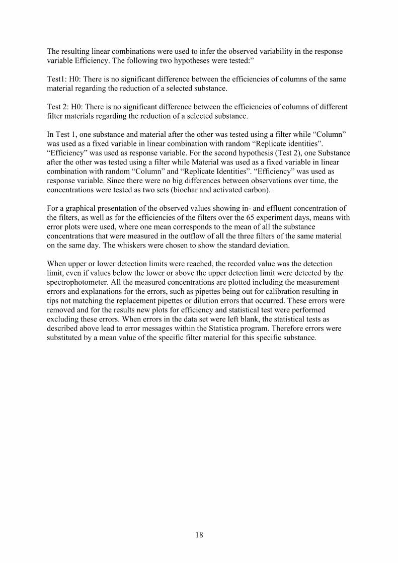
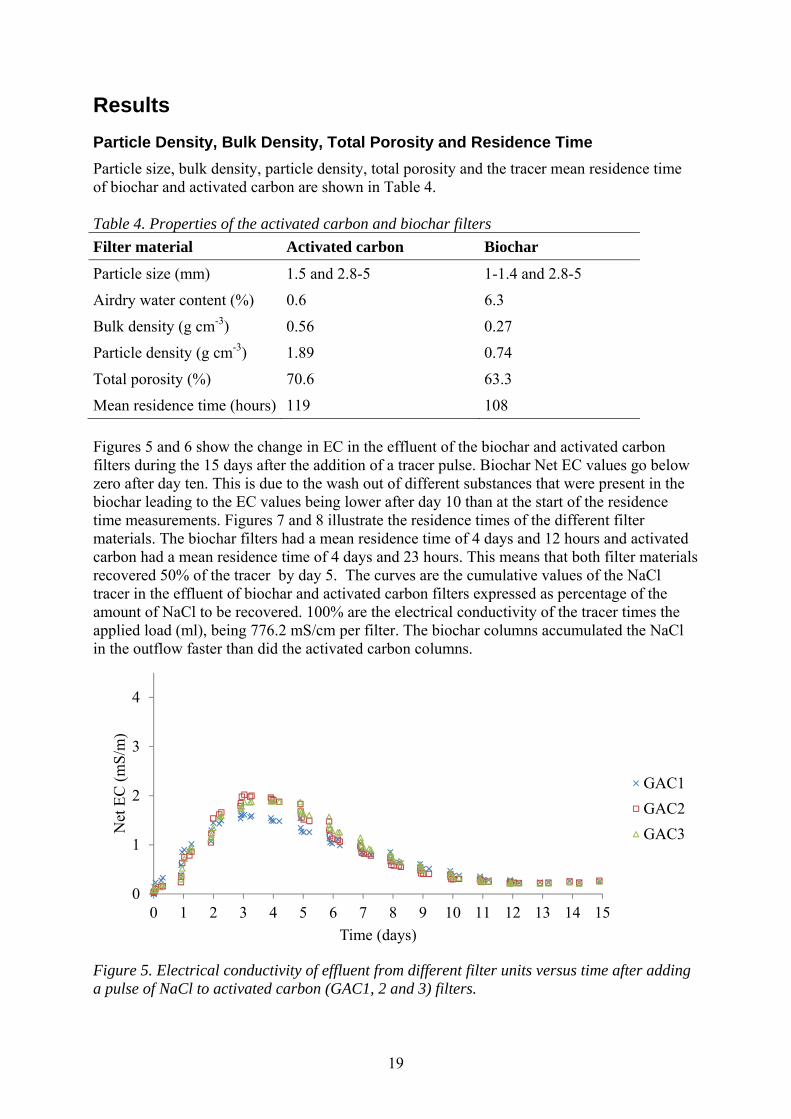
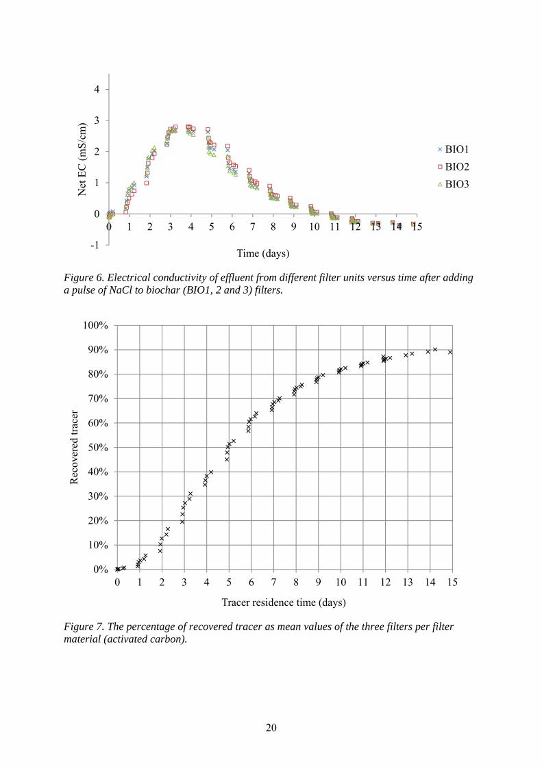
Figures 5 and 6 show the change in EC in the effluent of the biochar and activated carbon filters during the 15 days after the addition of a tracer pulse. Biochar Net EC values go below zero after day ten. This is due to the wash out of different substances that were present in the biochar leading to the EC values being lower after day 10 than at the start of the residence time measurements. Figures 7 and 8 illustrate the residence times of the different filter materials. The biochar filters had a mean residence time of 4 days and 12 hours and activated carbon had a mean residence time of 4 days and 23 hours. This means that both filter materials recovered 50% of the tracer by day 5. The curves are the cumulative values of the NaCl tracer in the effluent of biochar and activated carbon filters expressed as percentage of the amount of NaCl to be recovered. 100% are the electrical conductivity of the tracer times the applied load (ml), being 776.2 mS/cm per filter. The biochar columns accumulated the NaCl in the outflow faster than did the activated carbon columns.

Figure 5. Electrical conductivity of effluent from different filter units versus time after adding a pulse of NaCl to activated carbon (GAC1, 2 and 3) filters.

0

1

2

3

4

0 1 2 3 4 5 6 7 8 9 10 11 12 13 14 15

Net

EC

(m

S/m

)

Time (days)

GAC1

GAC2

GAC3

20

Figure 6. Electrical conductivity of effluent from different filter units versus time after adding a pulse of NaCl to biochar (BIO1, 2 and 3) filters.

Figure 7. The percentage of recovered tracer as mean values of the three filters per filter material (activated carbon).

-1

0

1

2

3

4

0 1 2 3 4 5 6 7 8 9 10 11 12 13 14 15

Net

EC

(m

S/c

m)

Time (days)

BIO1

BIO2

BIO3

0%

10%

20%

30%

40%

50%

60%

70%

80%

90%

100%

0 1 2 3 4 5 6 7 8 9 10 11 12 13 14 15

Rec

over

ed tr

acer

Tracer residence time (days)

21

Figure 8. The percentage of recovered tracer as mean values of the three filters per filter material (biochar).

Statistical tests

When testing the first null hypothesis, H0 (1): There is no significant difference, at 95% significance level, between the efficiencies of columns of the same material regarding the filtering of a selected substance, we can clearly see from the p-values in Table 5 that the hypothesis can be accepted. There is no significant difference between the efficiencies of the three filters filled with activated carbon, nor between the filters filled with biochar. This means that the three columns of each material performed similarly to the other columns of the same material regarding the efficiency of all tested substances. EC and pH were not included in the tests as efficiencies were not calculated for these parameters. When testing the second null hypothesis, H0 (2): There is no significant difference between the efficiencies of columns of different filter materials regarding the filtering of a selected substance, p-values in Table 6 show a significant difference between the performance of biochar and activated carbon regarding the efficiency in ammonium, total nitrogen, phosphate and total phosphorous removal. Regarding the efficiency in removal of the other parameters, there is no significant difference.

0%

10%

20%

30%

40%

50%

60%

70%

80%

90%

100%

0 1 2 3 4 5 6 7 8 9 10 11 12 13 14 15

Rec

over

ed tr

acer

Tracer residence time (days)

22

Table 5. Results (p-values) of mixed linear model (test 1). Activated carbon Biochar

NH4-N 0.510 0.919

COD 0.302 0.690

MBAS 0.896 0.297

NO3-N 0.997 0.487

Tot-N 0.990 0.436

PO4-P 0.657 0.982

Tot-P 0.710 0.920

Table 6. Results (p-values) of mixed linear model (test 2). Activated carbon vs. Biochar

NH4-N 0.000

COD 0.544

MBAS 0.501

NO3-N 0.208

Tot-N 0.021

PO4-P 0.000

Tot-P 0.000

Pollutants Concentrations and Treatment Efficiency: Overview

The pH, EC, MBAS, COD, Tot-P, PO4, Tot-N, NH4 and NO3 in the influent greywater are presented in Table 7. The mean and standard deviation of the efficiencies of the MBAS, COD, Tot-P, PO4, Tot-N, NH4 and NO3, as well as pH and EC mean values in biochar and activated carbon effluents over 65 days are presented in Table 8. The variation of the efficiencies of MBAS, COD, Tot-P, PO4, Tot-N, and NH4 for biochar and activated carbon filters are presented in Figures 9 and 10 respectively. These two scatter plots showing all measured parameters in one plot were made in Excel from the mean efficiencies of a filter material regarding one substance on one day. Table 7. Mean inflow concentrations for each filter material and measured substance Influent (mean) Stdv. n influent

pH 8.5 0.1 15

EC (mS/cm) 1.8 0.04 16

MBAS (mg/l) 82 15 32

COD (mg/l) 1389 100 40

Tot-P (mg/l) 3.6 0.1 41

PO4-P (mg/l) 2.6 0.1 41

Tot-N (mg/l) 95 6 40

NH4–N (mg/l) 3.7 0.5 42

NO3-N (mg/l) 1.3 0.2 42

23

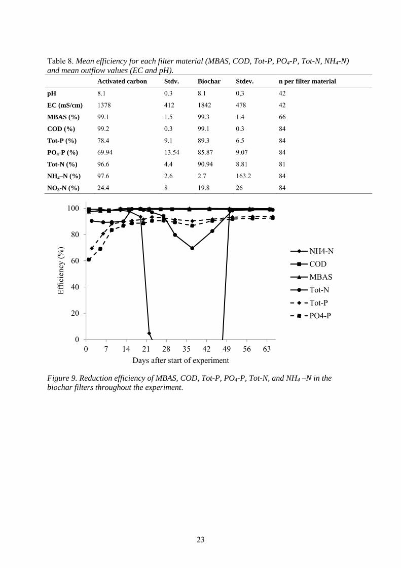
Table 8. Mean efficiency for each filter material (MBAS, COD, Tot-P, PO4-P, Tot-N, NH4-N) and mean outflow values (EC and pH). Activated carbon Stdv. Biochar Stdev. n per filter material

pH 8.1 0.3 8.1 0,3 42

EC (mS/cm) 1378 412 1842 478 42

MBAS (%) 99.1 1.5 99.3 1.4 66

COD (%) 99.2 0.3 99.1 0.3 84

Tot-P (%) 78.4 9.1 89.3 6.5 84

PO4-P (%) 69.94 13.54 85.87 9.07 84

Tot-N (%) 96.6 4.4 90.94 8.81 81

NH4–N (%) 97.6 2.6 2.7 163.2 84

NO3-N (%) 24.4 8 19.8 26 84

Figure 9. Reduction efficiency of MBAS, COD, Tot-P, PO4-P, Tot-N, and NH4 –N in the biochar filters throughout the experiment.

0

20

40

60

80

100

0 7 14 21 28 35 42 49 56 63

Eff

icie

ncy

(%)

Days after start of experiment

NH4-N

COD

MBAS

Tot-N

Tot-P

PO4-P

24

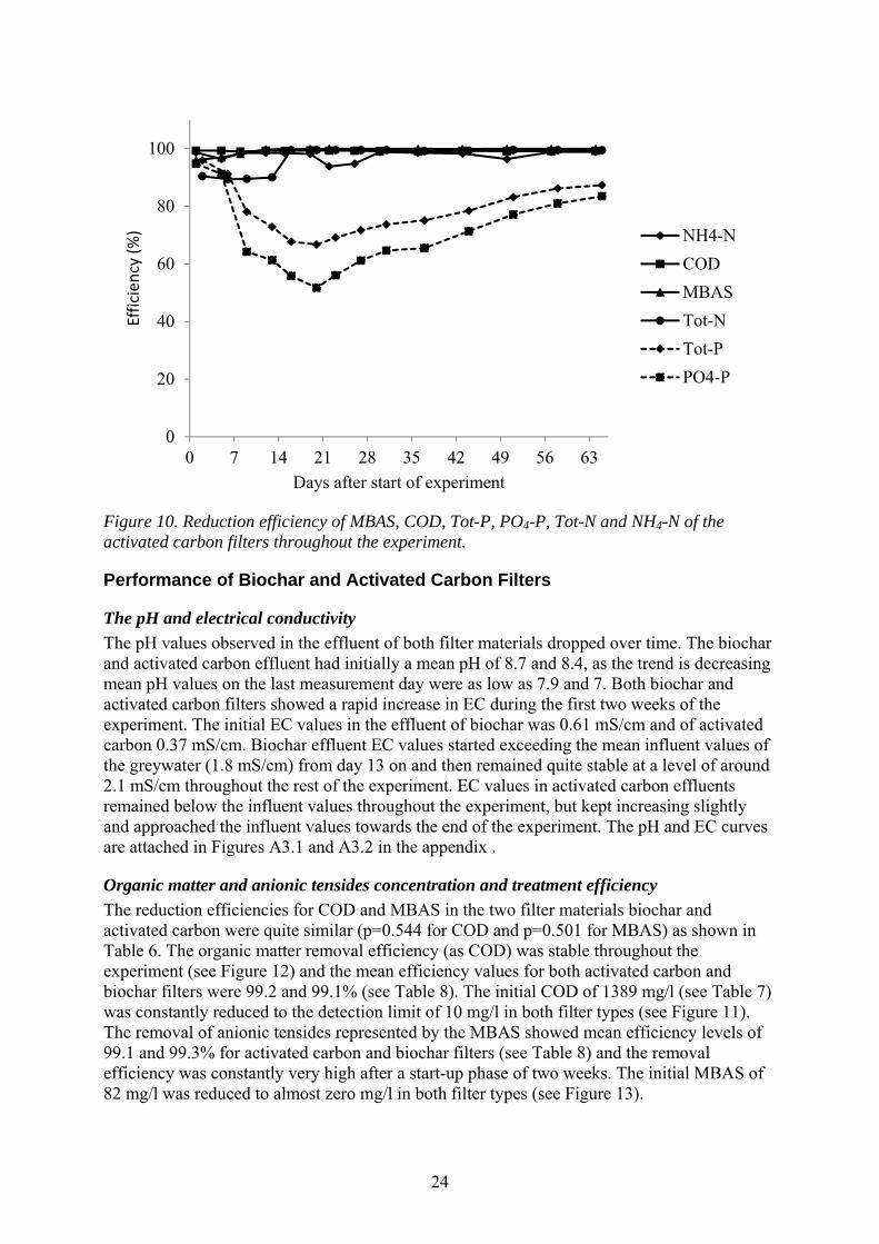
Figure 10. Reduction efficiency of MBAS, COD, Tot-P, PO4-P, Tot-N and NH4-N of the activated carbon filters throughout the experiment.

Performance of Biochar and Activated Carbon Filters

The pH and electrical conductivity

The pH values observed in the effluent of both filter materials dropped over time. The biochar and activated carbon effluent had initially a mean pH of 8.7 and 8.4, as the trend is decreasing mean pH values on the last measurement day were as low as 7.9 and 7. Both biochar and activated carbon filters showed a rapid increase in EC during the first two weeks of the experiment. The initial EC values in the effluent of biochar was 0.61 mS/cm and of activated carbon 0.37 mS/cm. Biochar effluent EC values started exceeding the mean influent values of the greywater (1.8 mS/cm) from day 13 on and then remained quite stable at a level of around 2.1 mS/cm throughout the rest of the experiment. EC values in activated carbon effluents remained below the influent values throughout the experiment, but kept increasing slightly and approached the influent values towards the end of the experiment. The pH and EC curves are attached in Figures A3.1 and A3.2 in the appendix .

Organic matter and anionic tensides concentration and treatment efficiency

The reduction efficiencies for COD and MBAS in the two filter materials biochar and activated carbon were quite similar (p=0.544 for COD and p=0.501 for MBAS) as shown in Table 6. The organic matter removal efficiency (as COD) was stable throughout the experiment (see Figure 12) and the mean efficiency values for both activated carbon and biochar filters were 99.2 and 99.1% (see Table 8). The initial COD of 1389 mg/l (see Table 7) was constantly reduced to the detection limit of 10 mg/l in both filter types (see Figure 11). The removal of anionic tensides represented by the MBAS showed mean efficiency levels of 99.1 and 99.3% for activated carbon and biochar filters (see Table 8) and the removal efficiency was constantly very high after a start-up phase of two weeks. The initial MBAS of 82 mg/l was reduced to almost zero mg/l in both filter types (see Figure 13).

0

20

40

60

80

100

0 7 14 21 28 35 42 49 56 63

Efficien

cy (%)


NH4-N

COD

MBAS

Tot-N

Tot-P

PO4-P

25

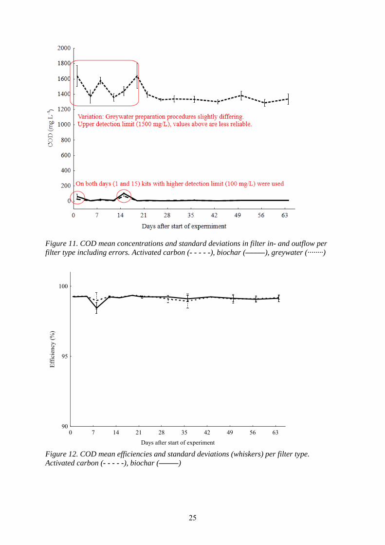
Figure 11. COD mean concentrations and standard deviations in filter in- and outflow per filter type including errors. Activated carbon (- - - - -), biochar (–––––), greywater (········)

0 7 14 21 28 35 42 49 56 63


90

95

100

Eff

icie

ncy

(%)

Figure 12. COD mean efficiencies and standard deviations (whiskers) per filter type. Activated carbon (- - - - -), biochar (–––––)

26

0 7 14 21 28 35 42 49 56 63


0

20

40

60

80

100

120M

BA

S (m

g L

-1)

Dilution error. Higher values can be assumed.

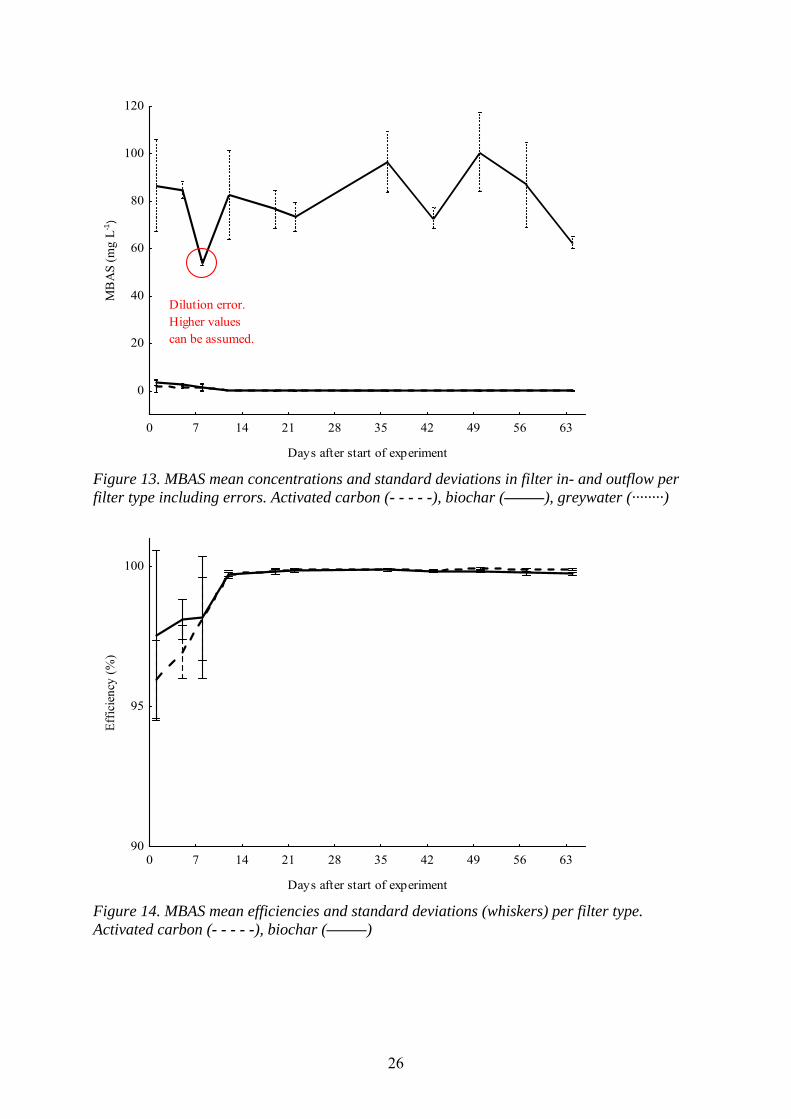
Figure 13. MBAS mean concentrations and standard deviations in filter in- and outflow per filter type including errors. Activated carbon (- - - - -), biochar (–––––), greywater (········)

0 7 14 21 28 35 42 49 56 63


90

95

100

Eff

icie

ncy

(%)

Figure 14. MBAS mean efficiencies and standard deviations (whiskers) per filter type. Activated carbon (- - - - -), biochar (–––––)

27

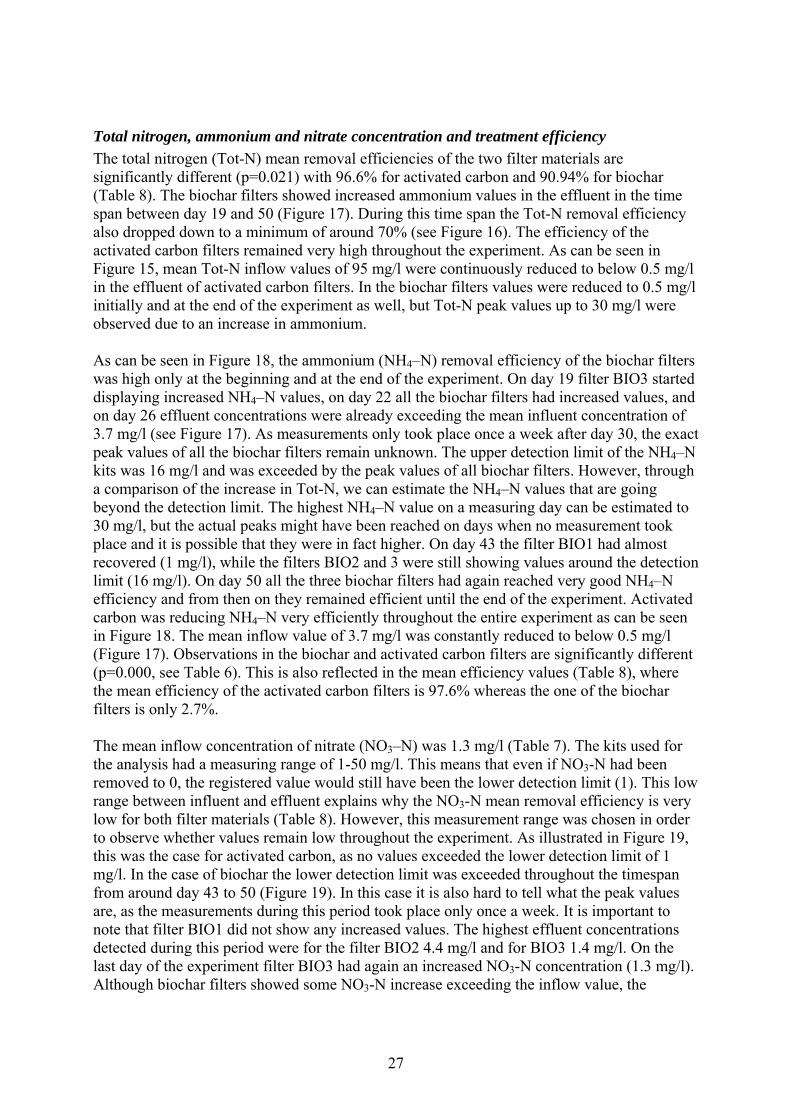
Total nitrogen, ammonium and nitrate concentration and treatment efficiency

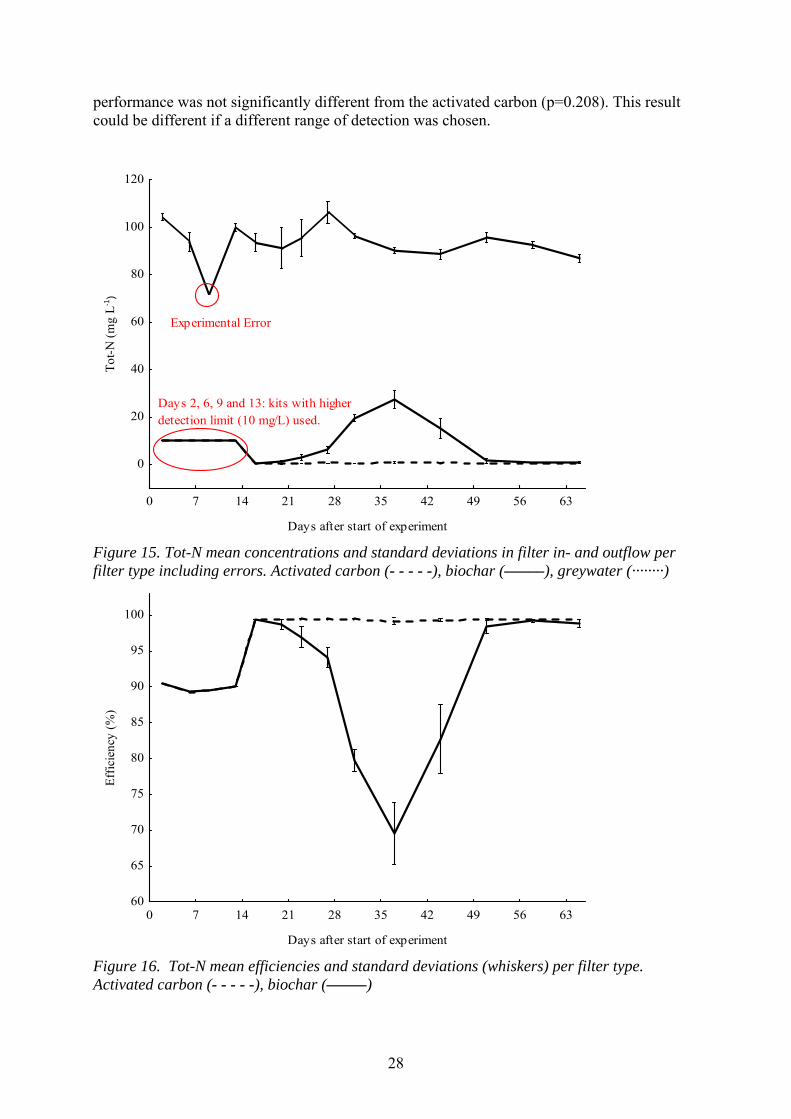
The total nitrogen (Tot-N) mean removal efficiencies of the two filter materials are significantly different (p=0.021) with 96.6% for activated carbon and 90.94% for biochar (Table 8). The biochar filters showed increased ammonium values in the effluent in the time span between day 19 and 50 (Figure 17). During this time span the Tot-N removal efficiency also dropped down to a minimum of around 70% (see Figure 16). The efficiency of the activated carbon filters remained very high throughout the experiment. As can be seen in Figure 15, mean Tot-N inflow values of 95 mg/l were continuously reduced to below 0.5 mg/l in the effluent of activated carbon filters. In the biochar filters values were reduced to 0.5 mg/l initially and at the end of the experiment as well, but Tot-N peak values up to 30 mg/l were observed due to an increase in ammonium. As can be seen in Figure 18, the ammonium (NH4–N) removal efficiency of the biochar filters was high only at the beginning and at the end of the experiment. On day 19 filter BIO3 started displaying increased NH4–N values, on day 22 all the biochar filters had increased values, and on day 26 effluent concentrations were already exceeding the mean influent concentration of 3.7 mg/l (see Figure 17). As measurements only took place once a week after day 30, the exact peak values of all the biochar filters remain unknown. The upper detection limit of the NH4–N kits was 16 mg/l and was exceeded by the peak values of all biochar filters. However, through a comparison of the increase in Tot-N, we can estimate the NH4–N values that are going beyond the detection limit. The highest NH4–N value on a measuring day can be estimated to 30 mg/l, but the actual peaks might have been reached on days when no measurement took place and it is possible that they were in fact higher. On day 43 the filter BIO1 had almost recovered (1 mg/l), while the filters BIO2 and 3 were still showing values around the detection limit (16 mg/l). On day 50 all the three biochar filters had again reached very good NH4–N

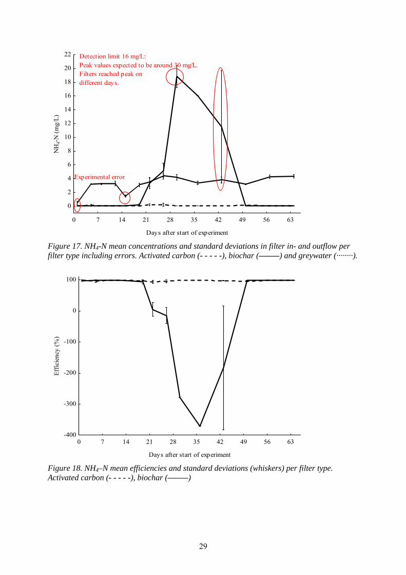
efficiency and from then on they remained efficient until the end of the experiment. Activated carbon was reducing NH4–N very efficiently throughout the entire experiment as can be seen in Figure 18. The mean inflow value of 3.7 mg/l was constantly reduced to below 0.5 mg/l (Figure 17). Observations in the biochar and activated carbon filters are significantly different (p=0.000, see Table 6). This is also reflected in the mean efficiency values (Table 8), where the mean efficiency of the activated carbon filters is 97.6% whereas the one of the biochar filters is only 2.7%. The mean inflow concentration of nitrate (NO3–N) was 1.3 mg/l (Table 7). The kits used for the analysis had a measuring range of 1-50 mg/l. This means that even if NO3-N had been removed to 0, the registered value would still have been the lower detection limit (1). This low range between influent and effluent explains why the NO3-N mean removal efficiency is very low for both filter materials (Table 8). However, this measurement range was chosen in order to observe whether values remain low throughout the experiment. As illustrated in Figure 19, this was the case for activated carbon, as no values exceeded the lower detection limit of 1 mg/l. In the case of biochar the lower detection limit was exceeded throughout the timespan from around day 43 to 50 (Figure 19). In this case it is also hard to tell what the peak values are, as the measurements during this period took place only once a week. It is important to note that filter BIO1 did not show any increased values. The highest effluent concentrations detected during this period were for the filter BIO2 4.4 mg/l and for BIO3 1.4 mg/l. On the last day of the experiment filter BIO3 had again an increased NO3-N concentration (1.3 mg/l). Although biochar filters showed some NO3-N increase exceeding the inflow value, the

28

performance was not significantly different from the activated carbon (p=0.208). This result could be different if a different range of detection was chosen.

0 7 14 21 28 35 42 49 56 63


0

20

40

60

80

100

120

Tot

-N (

mg

L-1

)

Days 2, 6, 9 and 13: kits with higher detection limit (10 mg/L) used.

Experimental Error

Figure 15. Tot-N mean concentrations and standard deviations in filter in- and outflow per filter type including errors. Activated carbon (- - - - -), biochar (–––––), greywater (········)

0 7 14 21 28 35 42 49 56 63


60

65

70

75

80

85

90

95

100

Eff

icie

ncy

(%)

Figure 16. Tot-N mean efficiencies and standard deviations (whiskers) per filter type. Activated carbon (- - - - -), biochar (–––––)

29

0 7 14 21 28 35 42 49 56 63


0

2

4

6

8

10

12

14

16

18

20

22N

H4-

N (

mg/

L)

Detection limit 16 mg/L:Peak values expected to be around 30 mg/L.Filters reached peak on different days.

Experimental error

Figure 17. NH4-N mean concentrations and standard deviations in filter in- and outflow per filter type including errors. Activated carbon (- - - - -), biochar (–––––) and greywater (········).

0 7 14 21 28 35 42 49 56 63


-400

-300

-200

-100

0

100

Eff

icie

ncy

(%)

Figure 18. NH4–N mean efficiencies and standard deviations (whiskers) per filter type. Activated carbon (- - - - -), biochar (–––––)

30

0 7 14 21 28 35 42 49 56 63


0

1

2

3N

O3-

N (

mg

L-1

)

Filters "BIO2" and "BIO3" had increased values (up to 2,4 mg/L)

Filter "BIO3" increased

to 1,5 mg L-1Experimental errors. 0,5 and 1 ml pipettes were out for calibration.

Experimental error. Two out of three greywater measurements were unusually high.

Figure 19. NO3-N mean concentrations and standard deviations in filter in- and outflow per filter type including errors. Activated carbon (- - - - -), biochar (–––––), greywater (········).

Total phosphorous and phosphate concentration and treatment efficiency

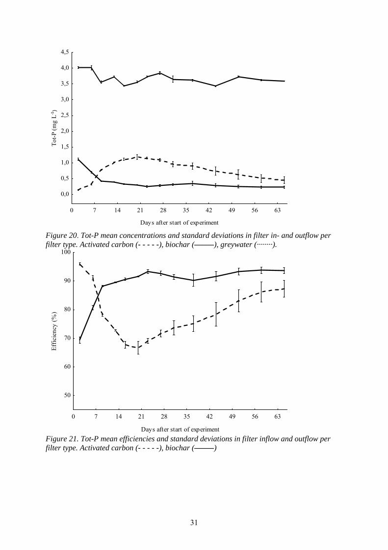
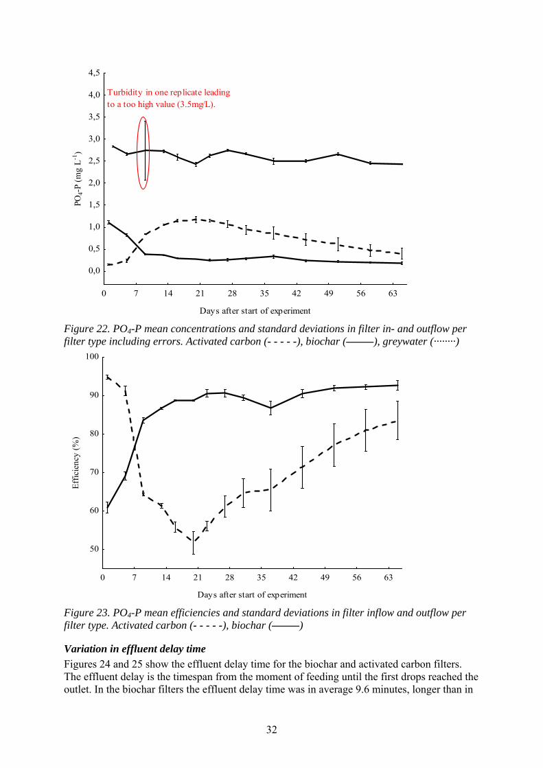
The efficiencies in total phosphorous (Tot-P) and phosphate (PO4-P) removal followed the same pattern throughout the experiment (see Figures 21 and 23). The performance of biochar and activated carbon filters was significantly different (p=0.000 for both Tot-P and PO4-P). At the beginning, the efficiency of the activated carbon filters was 94% for phosphate and 96% for total phosphorous, then values continually decreased and dropped down to 49% and 67% on day 20. On day 23 values started increasing again. The efficiency of the biochar filters was initially 62% for phosphate and 70% for total phosphorous, and then values continually increased until they reached a rather stable efficiency level of around 90% phosphate and 90-95% total phosphorous removal. As can be seen in Table 8, biochar has a mean efficiency of 86% and 89% for PO4-P and Tot-P whereas activated carbon reaches a mean of 70% and 78% respectively. As illustrated on Figures 22 and 24, the initial total phosphorous and phosphate concentration of 3.6 mg/l and 2.6 mg/l in the greywater were reduced to levels ranging from 0 to around 1 mg/l in the effluents of the biochar and activated carbon filters.

31

0 7 14 21 28 35 42 49 56 63


0,0

0,5

1,0

1,5

2,0

2,5

3,0

3,5

4,0

4,5T

ot-P

(m

g L

-1)

Figure 20. Tot-P mean concentrations and standard deviations in filter in- and outflow per filter type. Activated carbon (- - - - -), biochar (–––––), greywater (········).

0 7 14 21 28 35 42 49 56 63


50

60

70

80

90

100

Eff

icie

ncy

(%)

Figure 21. Tot-P mean efficiencies and standard deviations in filter inflow and outflow per filter type. Activated carbon (- - - - -), biochar (–––––)

32

0 7 14 21 28 35 42 49 56 63


0,0

0,5

1,0

1,5

2,0

2,5

3,0

3,5

4,0

4,5PO

4-P

(mg

L-1

)

Turbidity in one replicate leading to a too high value (3.5mg/L).

Figure 22. PO4-P mean concentrations and standard deviations in filter in- and outflow per filter type including errors. Activated carbon (- - - - -), biochar (–––––), greywater (········)

0 7 14 21 28 35 42 49 56 63


50

60

70

80

90

100

Eff

icie

ncy

(%)

Figure 23. PO4-P mean efficiencies and standard deviations in filter inflow and outflow per filter type. Activated carbon (- - - - -), biochar (–––––)

Variation in effluent delay time

Figures 24 and 25 show the effluent delay time for the biochar and activated carbon filters. The effluent delay is the timespan from the moment of feeding until the first drops reached the outlet. In the biochar filters the effluent delay time was in average 9.6 minutes, longer than in

33

the activated carbon filters where it took 3.9 minutes. During the first five weeks also Mondays and Tuesdays are plotted whereas in the last five weeks only Thursdays and Fridays are plotted. The filters were not fed with greywater during the weekends; therefore, on Mondays the outflow took more time to reach the outlet as the filters leached out over the weekend. This explains the peak effluent start values that were observed in both filter materials. Throughout the experiment the time it took until the first drops reached the outlet decreased for both filters.

Figure 24. Effluent delay time of the biochar filters throughout the experiment.

Figure 25. Effluent delay time of the activated carbon filters throughout the experiment

00:00

00:07

00:14

00:21

00:28

00:36

0 7 14 21 28 35 42 49 56 63

Eff

luen

t del

ay ti

me

(min

)


00:00

00:01

00:02

00:04

00:05

00:07

00:08

00:10

00:11

0 7 14 21 28 35 42 49 56 63

Eff

luen

t del

ay ti

me

(min

)


34

Discussion

Influence of Physical Parameters on Filter Performance

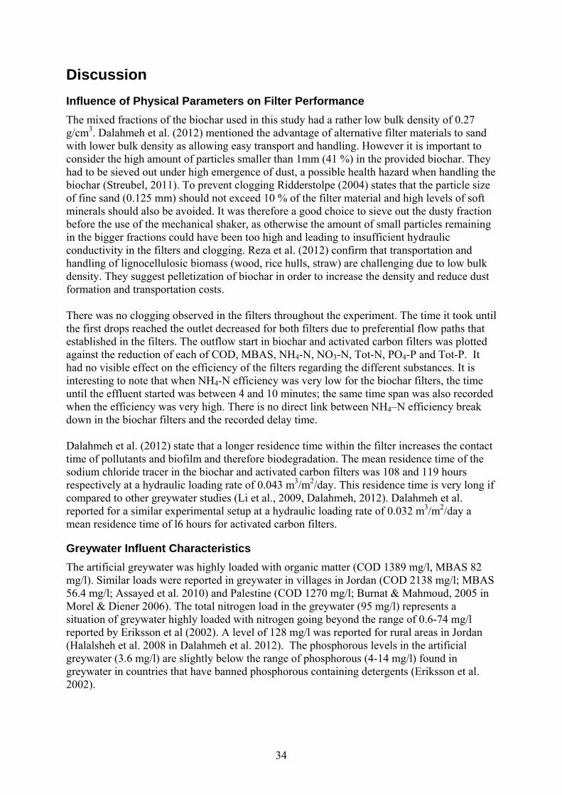
The mixed fractions of the biochar used in this study had a rather low bulk density of 0.27 g/cm3. Dalahmeh et al. (2012) mentioned the advantage of alternative filter materials to sand with lower bulk density as allowing easy transport and handling. However it is important to consider the high amount of particles smaller than 1mm (41 %) in the provided biochar. They had to be sieved out under high emergence of dust, a possible health hazard when handling the biochar (Streubel, 2011). To prevent clogging Ridderstolpe (2004) states that the particle size of fine sand (0.125 mm) should not exceed 10 % of the filter material and high levels of soft minerals should also be avoided. It was therefore a good choice to sieve out the dusty fraction before the use of the mechanical shaker, as otherwise the amount of small particles remaining in the bigger fractions could have been too high and leading to insufficient hydraulic conductivity in the filters and clogging. Reza et al. (2012) confirm that transportation and handling of lignocellulosic biomass (wood, rice hulls, straw) are challenging due to low bulk density. They suggest pelletization of biochar in order to increase the density and reduce dust formation and transportation costs. There was no clogging observed in the filters throughout the experiment. The time it took until the first drops reached the outlet decreased for both filters due to preferential flow paths that established in the filters. The outflow start in biochar and activated carbon filters was plotted against the reduction of each of COD, MBAS, NH4-N, NO3-N, Tot-N, PO4-P and Tot-P. It had no visible effect on the efficiency of the filters regarding the different substances. It is interesting to note that when NH4-N efficiency was very low for the biochar filters, the time until the effluent started was between 4 and 10 minutes; the same time span was also recorded when the efficiency was very high. There is no direct link between NH4–N efficiency break down in the biochar filters and the recorded delay time. Dalahmeh et al. (2012) state that a longer residence time within the filter increases the contact time of pollutants and biofilm and therefore biodegradation. The mean residence time of the sodium chloride tracer in the biochar and activated carbon filters was 108 and 119 hours respectively at a hydraulic loading rate of 0.043 m3/m2/day. This residence time is very long if compared to other greywater studies (Li et al., 2009, Dalahmeh, 2012). Dalahmeh et al. reported for a similar experimental setup at a hydraulic loading rate of 0.032 m3/m2/day a mean residence time of l6 hours for activated carbon filters.

Greywater Influent Characteristics

The artificial greywater was highly loaded with organic matter (COD 1389 mg/l, MBAS 82 mg/l). Similar loads were reported in greywater in villages in Jordan (COD 2138 mg/l; MBAS 56.4 mg/l; Assayed et al. 2010) and Palestine (COD 1270 mg/l; Burnat & Mahmoud, 2005 in Morel & Diener 2006). The total nitrogen load in the greywater (95 mg/l) represents a situation of greywater highly loaded with nitrogen going beyond the range of 0.6-74 mg/l reported by Eriksson et al (2002). A level of 128 mg/l was reported for rural areas in Jordan (Halalsheh et al. 2008 in Dalahmeh et al. 2012). The phosphorous levels in the artificial greywater (3.6 mg/l) are slightly below the range of phosphorous (4-14 mg/l) found in greywater in countries that have banned phosphorous containing detergents (Eriksson et al. 2002).

35

Organic Matter Removal

The 99% efficiency of both filter materials in removing COD and MBAS are similar to the efficiency (94% and 99% respectively) of activated carbon reported by Dalahmeh et al.(2012). As the efficiency was very high from the beginning on, the first process leading to the reduction of organic matter was probably adsorption. Over time a biofilm formed and biological activity contributed more and more to the organic matter removal (Lens et al., 1993, Dalahmeh et al., 2012). The treated greywater from both filter types of this experiment fulfills in terms of COD reduction all chosen examples of international wastewater reuse standards that are collected in Table 9.

Phosphorous Removal

The biochar performed better in total phosphorous removal than the activated carbon (89% and 78% respectively). The performance of the activated carbon filters in Dalahmeh et al. (2012) with 98% for phosphate removal was higher than the performance of the same material in this study (70%). The biochar in this study removed phosphate to 86%. It is important to consider that the total phosphorous concentration in the greywater was very low (3.6 mg/l) and that the filter performance may change under an increased load. The with biochar treated greywater fulfills the EU standard for discharge from urban wastewater treatment plants, the Italian standard for irrigation and urban reuse and -except for the first two weeks- also the Chinese standard for reuse in impoundments and lakes (see Table 9). The greywater treated by activated carbon always exceeded the threshold value (0.5 mg/l) of this Chinese standard, but it fulfilled the mentioned standards from the EU and Italy. The activated carbon used in this study and by Dalahmeh et al. (2012) has a very high specific surface area (>1000 m2/g) providing ample surface for adsorption (Dalahmeh et al. 2012). The specific surface area of the used biochar is unknown. Biochar surface areas are bigger than sand and comparable or higher than clay (5-750 m2/g) (Lehmann & Joseph, 2009). Streubel (2011) conducted an experiment using biochar to recover phosphorous in tanks from dairy effluent that had undergone prior anaerobic digestion. The effluent was filtered by a pressurized bio-filtration system filled with biochar as filter material. The parent material used for making the biochar in that study was anaerobically digested dairy manure fiber. The dairy effluent water was collected in a tank and then filtered over a period of 15 days. The mean initial phosphorous concentration was 546 mg/l and the mean reduction after 5 and 15 days was 63 and 70%. Although the design of this study and the filters were different from this study, the results are still relevant, as proving high efficiency of one biochar as filter material under very high loads of phosphorous.

Nitrogen Removal

Although the total nitrogen reduction in the biochar filters was not always stable, it was always efficient. Efficiency did not go below 70% and the mean efficiency was 91%. Activated carbon performance was stable in this experiment, and also in previous studies (Dalahmeh et al. 2012) and in average slightly more efficient (97% and 98% respectively) than biochar. The activated carbon filters fulfilled the wastewater reuse standards of the EU, Italy and China listed in Table 9. Total nitrogen values in the biochar effluent temporary went up to around 30 mg/l and therefore exceeded the threshold level of 15 mg/l as required for wastewater release in the EU, for irrigation in Italy or for reuse in lakes or impoundments in China.

36

The average ammonium reduction efficiency is very low for biochar (3%). However initially and towards the end of the experiment biochar performed as well as activated carbon. The greywater composition and feeding procedure remained the same throughout the whole experiment and there is no evidence for any human mistakes causing this phenomenon. It is possible that the ammonium was initially adsorbed by the biochar and that between day 19 and 22 the adsorption capacity of all biochar filters depleted, leading to NH4–N in the effluent. By day 50 all the biochar filters had recovered from the peak values and were again performing very efficiently. Eventually it took some time after the depletion of the adsorption capacity until the nitrifying bacteria grew and adapted. As nitrification occurred, NH4-N values went down again and the filters recovered. This hypothesis cannot be supported at this point of time. It would be interesting for further studies to investigate on the adsorption capacity of biochar for ammonium. Table 9. International Wastewater Reuse Standards EU Jordan Egypt Italy China

COD

125 mg/l

100 mg/l

40 mg/l

100 mg/l

Anionic surfactants

100 mg/l 0.5 mg/l

Tot-P 1-2 mg/l 2 mg/l 0.5 mg/l

Tot-N 10-15 mg/l 15 mg/l 15 mg/l

NH4 5 mg/l

EC 1500

pH

6-9 6-9.5 6-9

Reuse Discharge from urban wastewater treatment plants

Reclaimed domestic reuse

Unrestricted irrigation

Irrigation, urban reuse

Impoundments and lakes

Source Council Directive (1991)

Dalahmeh et al. (2011)

Smith & Bani-Melhem (2012)

Chaillou et al. (2009)

Ernst et al. (2006)

37

Conclusions

1. Concerning the filter efficiency, both materials tested high for all parameters (COD, MBAS, Tot-N, NO3-N, NH4-N, Tot-P, PO4-P), except biochar for NH4-N efficiency. Regarding the reduction of organic matter both filter materials had equal performance. For the reduction of total phosphorous and phosphate, biochar performed superior to the activated carbon and for the removal of total nitrogen activated carbon performed slightly superior to biochar due to some processes leading to a temporary ammonium nitrogen efficiency drop in the biochar effluent.

2. The equal performance in organic matter and total phosphorous filtering from greywater suggests that the investigated biochar can function as alternative to activated carbon for organic matter and phosphorous removal. Biochar even showed superior phosphorous removal.

3. Further research on the biochar performance under increased hydraulic load and higher phosphorous load is recommended. It is also relevant to investigate on the efficiency of the biochar over a longer period of time and to test and compare the performance of biochars derived from different parent materials. Regarding biochar recycling it is of interest to investigate on the effects of the application of the used biochar filter material to soils.

38

References

Ahsan, S., Kaneco, S., Ohta, K., Mizuno, T., Kani, K. 2001. Use of some natural and waste materials for waste water treatment. Water Research, 35, 3738–3742.

Al-Jayyousi, O.R., 2003, Greywater reuse: towards sustainable water management. Desalination. 156 , 181-192. Assayed, M., Dalahmeh, S., Suleiman, W., 2010. Onsite Greywater Treatment Using Septic Tank Followed by

Intermittent Sand Filter- A Case Study of Abu Al Farth Village in Jordan. International Journal of Chemical and Environmental Engineering, 1(1), 67-71.

Carpenter, S.R., Caraco, N.F., Correll, D.L., Howarth, R.W., Sharpley, A.N., Smith, V.H., 1998. Nonpoint

pollution of surface waters with phosphorous and nitrogen. Ecological Applications 8, 559–568. Chaillou, K., Gérente, C., Andrès, Y., Wolbert, D. 2009. Bathroom greywater characterization and potential

treatments for reuse. Water Air Soil Pollution. 215, 31-42. Council Directive (EC) 1991/271/EEC of 21 May 1991 concerning urban waste water teatment. Published at:

http://eur-lex.europa.eu/LexUriServ/LexUriServ.do?uri=OJ:L:1991:135:0040:0052:EN:PDF (1.7.2012) Dalahmeh, S.S., Pell, M., Vinneras, B., Hylander, L.D., Oborn, I., Jonsson, H., 2012. Efficiency of bark,

activated charcoal, foam and sand filters in reducing pollutants from greywater. Water, Air, & Soil Pollution, 1–15.

Dalahmeh, S.S., Hylander, L.D., Vinneras, B., Pell, M., Oborn, I., Jonsson, H., 2011. Potential of organic filter

materials for treating greywater to achieve irrigation quality: a review. Water Science & Technology, 63, 1832–1840.

Eriksson, E., Auffarth, K., Henze, M., Ledin, A. 2002.Characteristics of grey wastewater. Urban Water, 4 (1), 85-

104. Erns,t M., Sperlich, A., Zheng, X., Gan, Y., Hu, J., Zhao, X., Wang, J., Jekel, M. 2007. An integrated wastewater

treatment and reuse concept for the Olympic Park 2008, Beijing. Desalination, 202(1-3), 293–301. Gross, A. et al. 2005. Environmental impact and health risks associated with greywater irrigation: a case study.

Water Science and Technology, 52(8), 161-169. Halalsheh, M., Dalahmeh, S., Sayed, M., Suleiman, W., Shareef, M., Mansour, M., Safi, M., 2008. Grey water

characteristics and treatment options for rural areas in Jordan. Bioresource Technology, 99, 6635–6641. Hillel, D. 1982. Introduction to Soil Physics. Academic Press Inc. Internationan Biochar Initiative. 2012. IBI member network. Regional biochar groups. http://www.biochar-

international.org/network/communities (28.4.2012) Lehmann, J., Joseph, S., 2009. Biochar for Environmental Management: Science and Technology. Earthscan. Li, F., Wichmann, K., Otterpohl, R. 2009. Review of the technological approaches for greywater treatment and

reuses. Science of the Total Environment, 407(11), 3439-3449. Morel, A., Diener, S. 2006. Greywater management in low and middle-income countries: review of different

treatment systems for households or neighbourhoods. Swiss Federal Institute of Aquatic Science and Technology Eawag.

Palmquist, H., Hanæus, J., 2005. Hazardous substances in separately collected grey- and blackwater from

ordinary Swedish households. Science of the Total Environment, 348, 151–163. Reza, M., Lynam, J., Vasquez, V., Coronella, C., 2012. Pelletization of biochar from hydrothermally carbonized

wood.Environmental Progress & Sustainable Energy, 31(2), 225-234.

39

Ridderstolpe, P., 2004. Introduction to greywater management. EcoSanRes Publication Series. Stockholm Environment Institute, Stockholm.

Simetric, 2012. Table of Density of Pure and Tap Water and Specific Gravity. Published at:

http://www.simetric.co.uk/si_water.htm (05.04.2012) Smith, E., Bani-Melhem, K., 2012. Grey water characterization and treatment for reuse in an arid environment.

Water Science & Technology, 66(1), 72-78.

Steiner, C., 2007. Slash and Char as Alternative to Slash and Burn: Soil Charcoal Amendments Maintain Soil Fertility and Establish a Carbon Sink. Cuvillier Verlag.

Streubel, J., 2011. Biochar: Its Characterization and Utility for Recovering Phosphorous from Anaerobic

Digested Dairy Effluent. Dissertation. Washington State University. Published at: http://research.wsulibs.wsu.edu/xmlui/bitstream/handle/2376/2891/Streubel_wsu_0251E_10131.pdf?sequence=1

Tanaka, M., Girard, G., Davis, R., Peuto, A., Bignell, N. 2011. Recommended table for the density of water

between 0°C and 40°C based on recent experimental reports. Metrologia 38, 301 Velten, S. 2008. Adsorption capacity and biological activity of biological activated carbon filters in drinking

water treatment. ETH. http://dx.doi.org/10.3929/ethz-a-005820821

40

Appendices

Appendix 1. Fractions of the sieved biochar

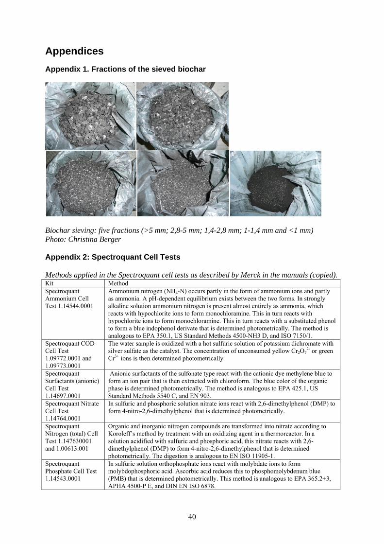
Biochar sieving: five fractions (>5 mm; 2,8-5 mm; 1,4-2,8 mm; 1-1,4 mm and <1 mm) Photo: Christina Berger Appendix 2: Spectroquant Cell Tests Methods applied in the Spectroquant cell tests as described by Merck in the manuals (copied). Kit Method Spectroquant Ammonium Cell Test 1.14544.0001

Ammonium nitrogen (NH4-N) occurs partly in the form of ammonium ions and partly as ammonia. A pH-dependent equilibrium exists between the two forms. In strongly alkaline solution ammonium nitrogen is present almost entirely as ammonia, which reacts with hypochlorite ions to form monochloramine. This in turn reacts with hypochlorite ions to form monochloramine. This in turn reacts with a substituted phenol to form a blue indophenol derivate that is determined photometrically. The method is analogous to EPA 350.1, US Standard Methods 4500-NH3 D, and ISO 7150/1.

Spectroquant COD Cell Test 1.09772.0001 and 1.09773.0001

The water sample is oxidized with a hot sulfuric solution of potassium dichromate with silver sulfate as the catalyst. The concentration of unconsumed yellow Cr2O7

2- or green Cr3+ ions is then determined photometrically.

Spectroquant Surfactants (anionic) Cell Test 1.14697.0001

Anionic surfactants of the sulfonate type react with the cationic dye methylene blue to form an ion pair that is then extracted with chloroform. The blue color of the organic phase is determined photometrically. The method is analogous to EPA 425.1, US Standard Methods 5540 C, and EN 903.

Spectroquant Nitrate Cell Test 1.14764.0001

In sulfuric and phosphoric solution nitrate ions react with 2,6-dimethylphenol (DMP) to form 4-nitro-2,6-dimethylphenol that is determined photometrically.

Spectroquant Nitrogen (total) Cell Test 1.147630001 and 1.00613.001

Organic and inorganic nitrogen compounds are transformed into nitrate according to Koroleff’s method by treatment with an oxidizing agent in a thermoreactor. In a solution acidified with sulfuric and phosphoric acid, this nitrate reacts with 2,6-dimethylphenol (DMP) to form 4-nitro-2,6-dimethylphenol that is determined photometrically. The digestion is analogous to EN ISO 11905-1.

Spectroquant Phosphate Cell Test 1.14543.0001

In sulfuric solution orthophosphate ions react with molybdate ions to form molybdophosphoric acid. Ascorbic acid reduces this to phosphomolybdenum blue (PMB) that is determined photometrically. This method is analogous to EPA 365.2+3, APHA 4500-P E, and DIN EN ISO 6878.

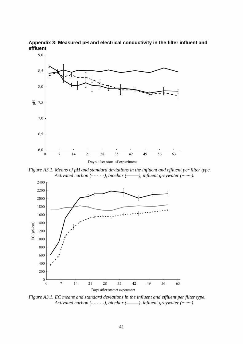
41

Appendix 3: Measured pH and electrical conductivity in the filter influent and effluent

0 7 14 21 28 35 42 49 56 63


6,0

6,5

7,0

7,5

8,0

8,5

9,0

pH

Figure A3.1. Means of pH and standard deviations in the influent and effluent per filter type.

Activated carbon (- - - - -), biochar (–––––), influent greywater (········).

0 7 14 21 28 35 42 49 56 63


0

200

400

600

800

1000

1200

1400

1600

1800

2000

2200

2400

EC

(µ

S/c

m)

Figure A3.1. EC means and standard deviations in the influent and effluent per filter type.

Activated carbon (- - - - -), biochar (–––––), influent greywater (········).

SLU

Institutionen för energi och teknik

Box 7032

75007 UPPSALA

Tel. 018-67 1O 00

www.slu.se/energyandtechnology

SLU

Department of Energy and Technology

Box 7032

S-75007 UPPSALA

SWEDEN Phone +46 18 671000

http://www.slu.se/

Biochar and activated carbon filters for greywater...

Documents

Transcript of Biochar and activated carbon filters for greywater...