Slide 1Copyright © 2007 Pearson Education, Inc Publishing as Pearson Addison-Wesley.

A

Presentation On

Binomial Probability Distributions

By

Tayab Ali (M/12/ME-11)

ME- Industrial and Production

Jorhat Engineering College

Slide 2

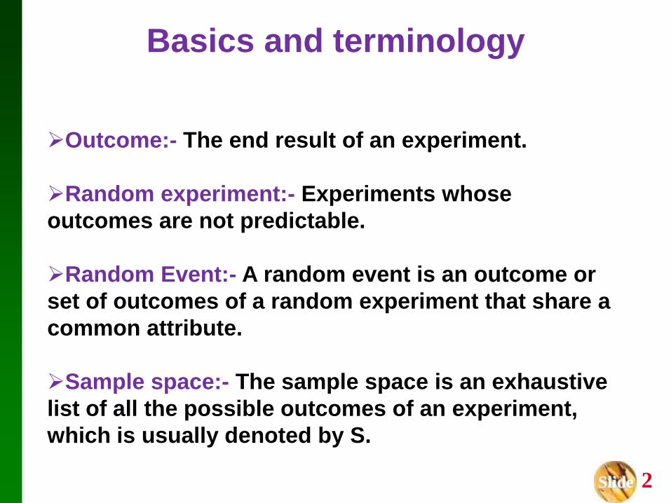
Outcome:- The end result of an experiment.

Random experiment:- Experiments whose

outcomes are not predictable.

Random Event:- A random event is an outcome or

set of outcomes of a random experiment that share a

common attribute.

Sample space:- The sample space is an exhaustive

list of all the possible outcomes of an experiment,

which is usually denoted by S.

Basics and terminology

Slide 3

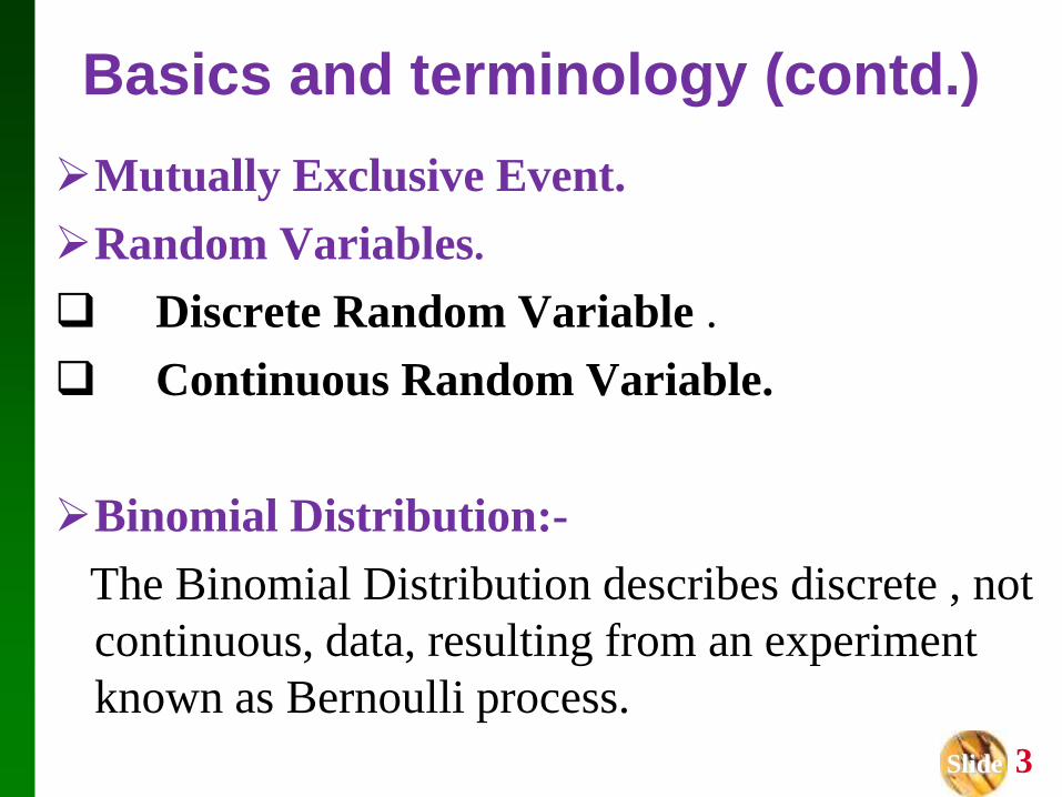
Basics and terminology (contd.)

Mutually Exclusive Event.

Random Variables.

Discrete Random Variable .

Continuous Random Variable.

Binomial Distribution:-

The Binomial Distribution describes discrete , not

continuous, data, resulting from an experiment

known as Bernoulli process.

Slide 4

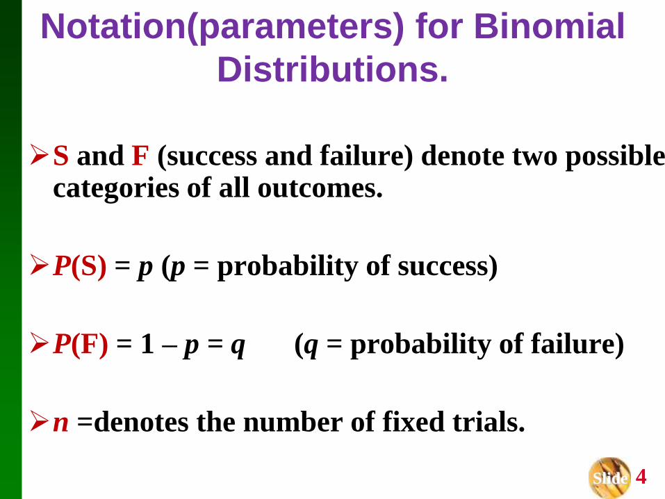
Notation(parameters) for Binomial

Distributions.

S and F (success and failure) denote two possible categories of all outcomes.

P(S) = p (p = probability of success)

P(F) = 1 – p = q (q = probability of failure)

n =denotes the number of fixed trials.

Slide 5

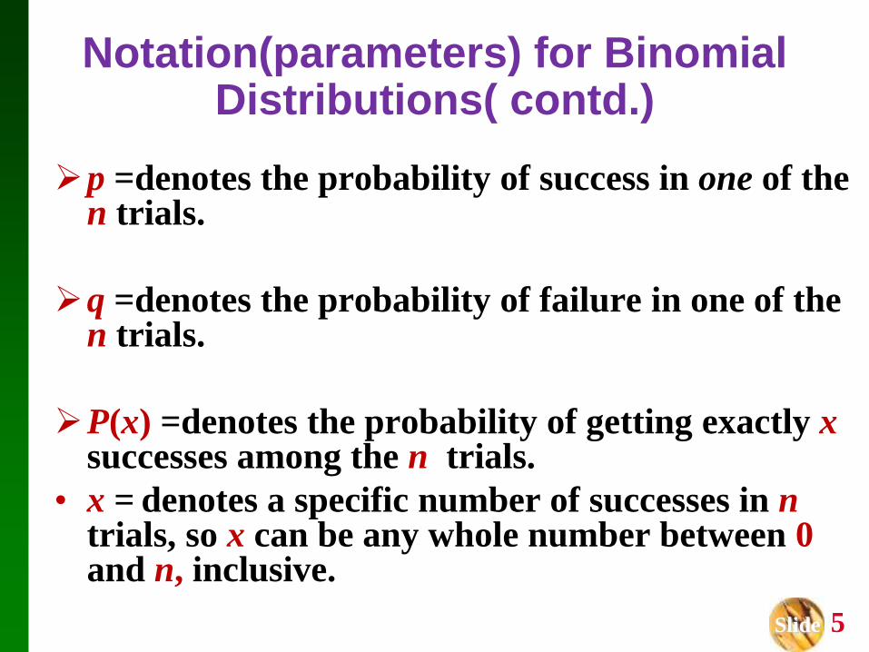
Notation(parameters) for Binomial Distributions( contd.)

p =denotes the probability of success in one of the n trials.

q =denotes the probability of failure in one of the n trials.

P(x) =denotes the probability of getting exactly xsuccesses among the n trials.

• x = denotes a specific number of successes in ntrials, so x can be any whole number between 0 and n, inclusive.

Slide 6

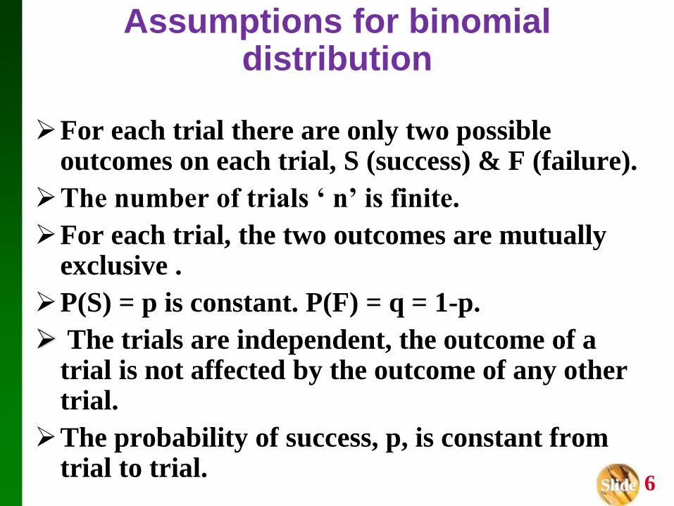
Assumptions for binomial distribution

For each trial there are only two possible outcomes on each trial, S (success) & F (failure).

The number of trials ‘ n’ is finite.

For each trial, the two outcomes are mutually exclusive .

P(S) = p is constant. P(F) = q = 1-p.

The trials are independent, the outcome of a trial is not affected by the outcome of any other trial.

The probability of success, p, is constant from trial to trial.

Slide 7

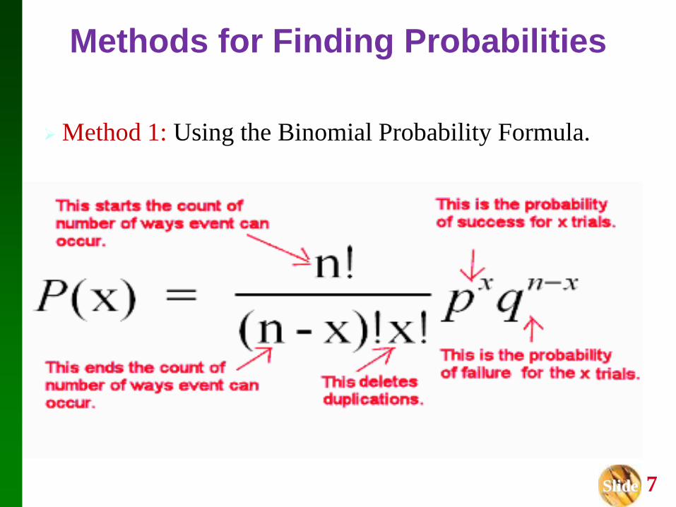
Methods for Finding Probabilities

Method 1: Using the Binomial Probability Formula.

Slide 8

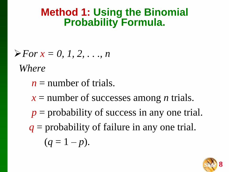
Method 1: Using the Binomial Probability Formula.

For x = 0, 1, 2, . . ., n

Where

n = number of trials.

x = number of successes among n trials.

p = probability of success in any one trial.

q = probability of failure in any one trial.

(q = 1 – p).

Slide 9

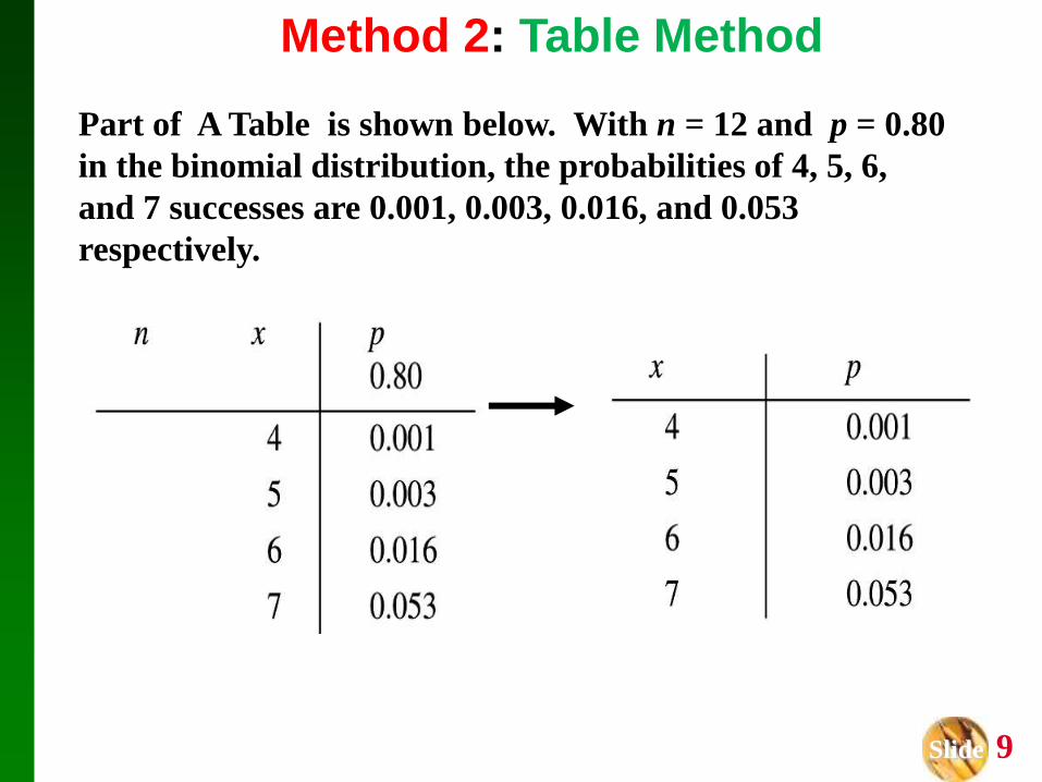
Method 2: Table Method

Part of A Table is shown below. With n = 12 and p = 0.80

in the binomial distribution, the probabilities of 4, 5, 6,

and 7 successes are 0.001, 0.003, 0.016, and 0.053

respectively.

Slide 10

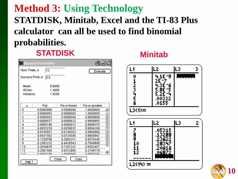
Method 3: Using TechnologySTATDISK, Minitab, Excel and the TI-83 Plus

calculator can all be used to find binomial

probabilities.STATDISK Minitab

Slide 11

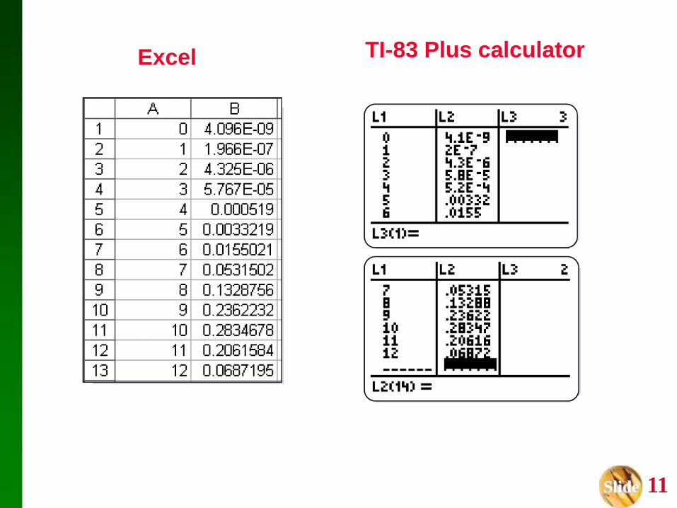
Excel TI-83 Plus calculator

Slide 12

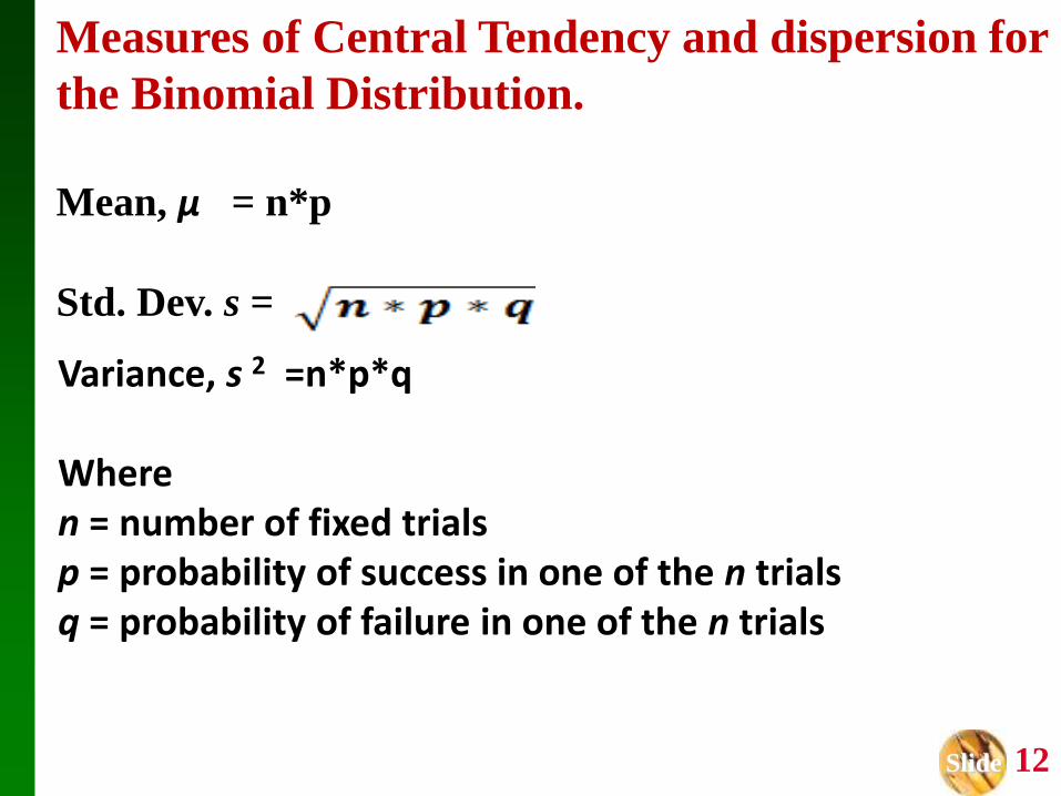
Measures of Central Tendency and dispersion for

the Binomial Distribution.

Mean, µ = n*p

Std. Dev. s =

Variance, s 2 =n*p*q

Wheren = number of fixed trialsp = probability of success in one of the n trialsq = probability of failure in one of the n trials

Slide 13

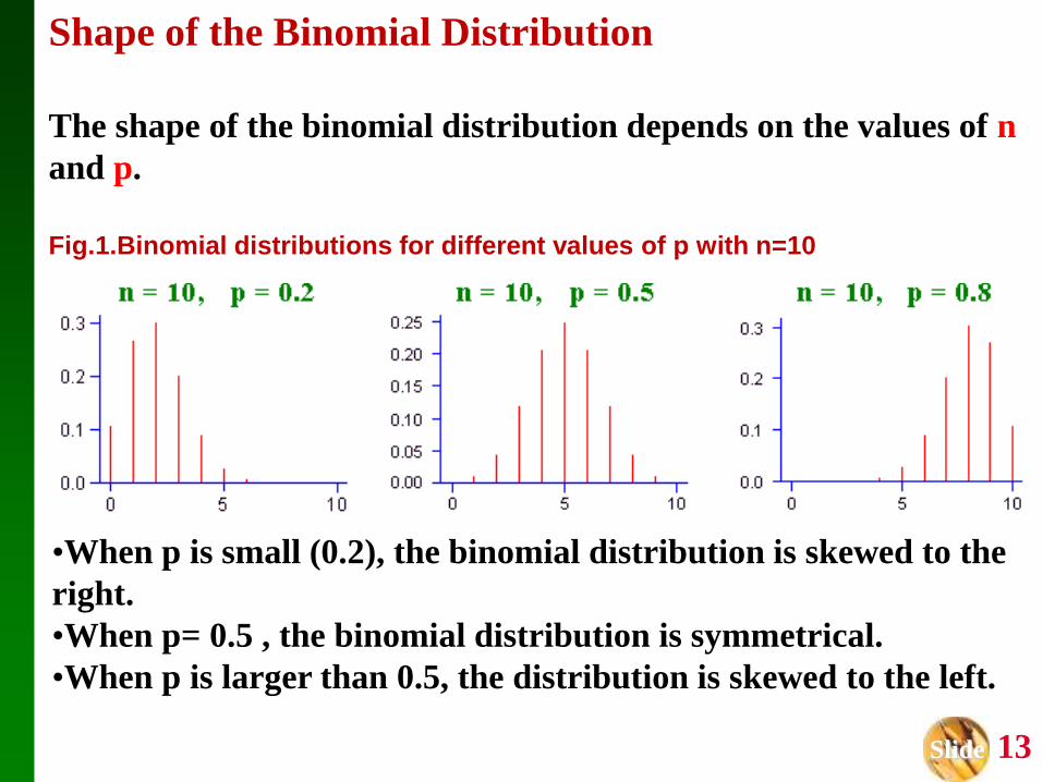
Shape of the Binomial Distribution

The shape of the binomial distribution depends on the values of n

and p.

Fig.1.Binomial distributions for different values of p with n=10

•When p is small (0.2), the binomial distribution is skewed to the

right.

•When p= 0.5 , the binomial distribution is symmetrical.

•When p is larger than 0.5, the distribution is skewed to the left.

Slide 14

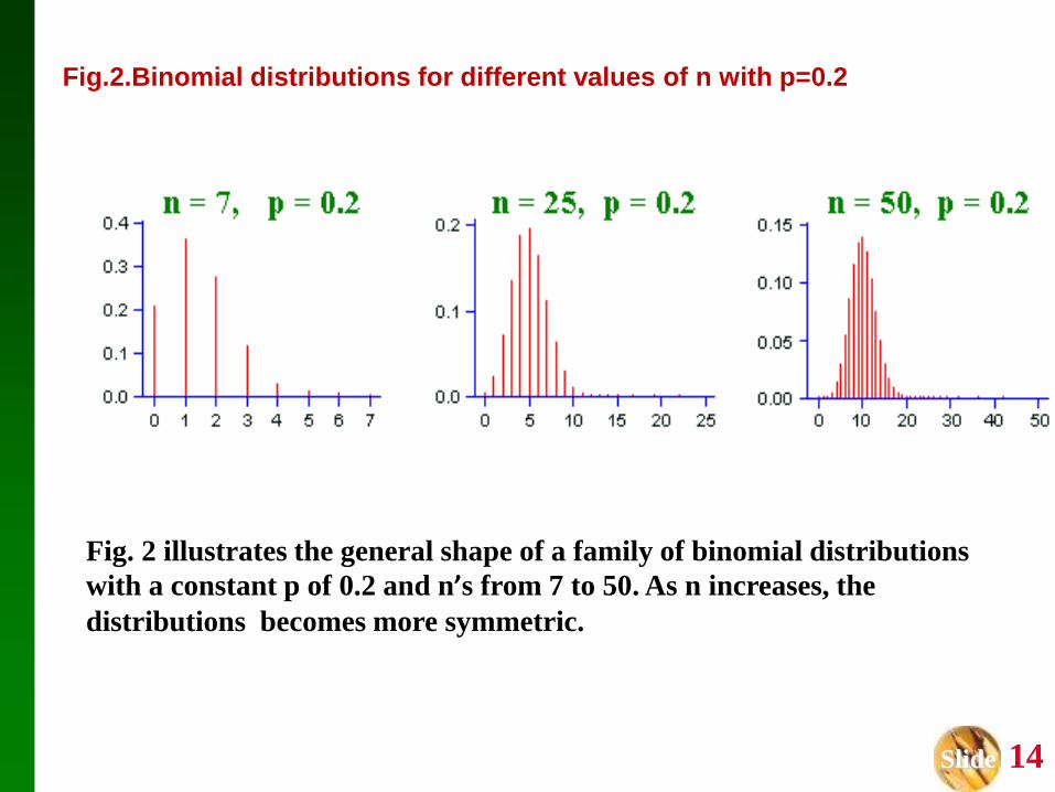
Fig.2.Binomial distributions for different values of n with p=0.2

Fig. 2 illustrates the general shape of a family of binomial distributions

with a constant p of 0.2 and n’s from 7 to 50. As n increases, the

distributions becomes more symmetric.

Slide 15

Applications for binomial distributions

Binomial distributions describe the possible number of times that

a particular event will occur in a sequence of observations.

They are used when we want to know about the occurrence of an

event, not its magnitude.

• In a clinical trial, a patient’s condition may improve or not. We study

the number of patients who improved, not how much better they feel.

•Is a person ambitious or not? The binomial distribution describes the

number of ambitious persons, not how ambitious they are.

•In quality control we assess the number of defective items in a lot of

goods, irrespective of the type of defect.

Examples

Slide 16

Areas of Application

• Common uses of binomial distributions in business include quality

control. Industrial engineers are interested in the proportion of

defectives .

• Also used extensively for medical (survive, die)

• It is also used in military applications (hit, miss).

Slide 17

Thank You