Binomial Random Binomial Random VariablesVariables

Binomial Probability Distributions

Binomial Random Binomial Random VariablesVariables

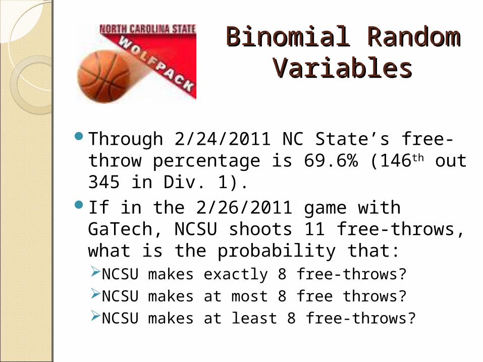
Through 2/24/2011 NC State’s free-throw percentage is 69.6% (146th out 345 in Div. 1).

If in the 2/26/2011 game with GaTech, NCSU shoots 11 free-throws, what is the probability that:NCSU makes exactly 8 free-throws?NCSU makes at most 8 free throws?NCSU makes at least 8 free-throws?

““2-outcome” situations are 2-outcome” situations are very commonvery common

Heads/tailsDemocrat/RepublicanMale/FemaleWin/LossSuccess/FailureDefective/Nondefective

Probability Model for this Probability Model for this Common SituationCommon Situation

Common characteristics◦repeated “trials”◦2 outcomes on each trial

Leads to Binomial Experiment

Binomial ExperimentsBinomial Experimentsn identical trials

◦n specified in advance2 outcomes on each trial

◦usually referred to as “success” and “failure”

p “success” probability; q=1-p “failure” probability; remain constant from trial to trial

trials are independent

Binomial Random VariableBinomial Random VariableThe binomial random variable X is the number of “successes” in the n trials

Notation: X has a B(n, p) distribution, where n is the number of trials and p is the success probability on each trial.

ExamplesExamples

a. Yes; n=10; success=“major repairs within 3 months”; p=.05

b. No; n not specified in advancec. No; p changesd. Yes; n=1500; success=“chip is

defective”; p=.10

Binomial Probability Binomial Probability DistributionDistribution

0 0

trials, success probability on each trial

probability distribution:

( ) , 0,1,2, ,

( ) ( )

( ) (

x n xn x

n nn x n xx

x x

n p

p x C p q x n

E x xp x x p q np

Var x E x npq

P(x) = • px • qn-xn ! (n – x )!x!

Number of outcomes with

exactly x successes

among n trials

Rationale for the Binomial Probability Formula

P(x) = • px • qn-xn ! (n – x )!x!

Number of outcomes with

exactly x successes

among n trials

Probability of x successes

among n trials for any one

particular order

Binomial Probability Formula

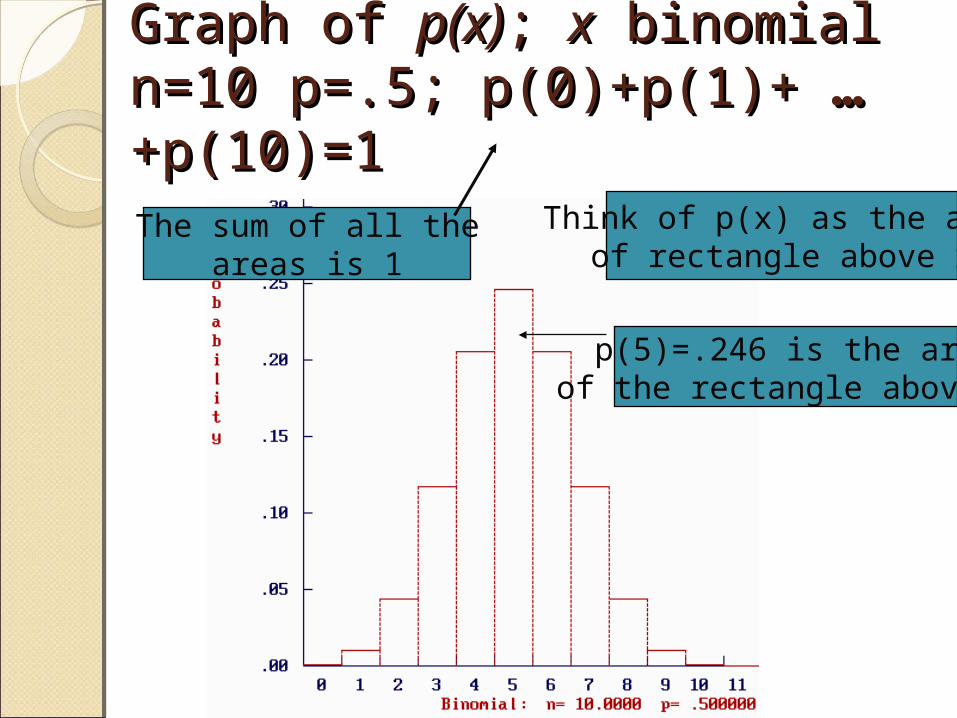
Graph of Graph of p(x)p(x); ; xx binomial binomial n=10 p=.5; p(0)+p(1)+ n=10 p=.5; p(0)+p(1)+ …… +p(10)=1+p(10)=1

Think of p(x) as the areaof rectangle above x

p(5)=.246 is the areaof the rectangle above 5

The sum of all theareas is 1

Binomial Probability Histogram: n=100, p=.5

0

0.01

0.02

0.03

0.04

0.05

0.06

0.07

0.08

0.09

Binomial Probability Histogram: n=100, p=.95

0

0.01

0.02

0.03

0.04

0.05

0.06

0.07

0.08

0.09

0.1

0.11

0.12

0.13

0.14

0.15

0.16

0.17

0.18

70 72 74 76 78 80 82 84 86 88 90 92 94 96 98 100

ExampleExample

A production line produces motor housings, 5% of which have cosmetic defects. A quality control manager randomly selects 4 housings from the production line. Let x=the number of housings that have a cosmetic defect. Tabulate the probability distribution for x.

SolutionSolution(i) D=defective, G=goodoutcome x P(outcome)GGGG 0 (.95)(.95)(.95)(.95)DGGG 1 (.05)(.95)(.95)(.95)GDGG 1 (.95)(.05)(.95)(.95) : : :DDDD 4 (.05)4

SolutionSolution

0 44 0

1 34 1

2 24 2

3 14 3

44 4

( ) is a binomial random variable

( ) , 0,1,2, ,

4, .05 ( .95)

(0) (.05) (.95) .815

(1) (.05) (.95) .171475

(2) (.05) (.95) .01354

(3) (.05) (.95) .00048

(4) (.05) (.9

x n xn x

ii x

p x C p q x n

n p q

p C

p C

p C

p C

p C

05) .00000625

SolutionSolution

x 0 1 2 3 4p(x) .815

.171475 .01354 .00048 .00000625

Example (cont.)Example (cont.)

x 0 1 2 3 4p(x) .815

.171475 .01354 .00048 .00000625

What is the probability that at least 2 of the housings will have a cosmetic defect?

P(x p(2)+p(3)+p(4)=.01402625

Example (cont.)Example (cont.)

What is the probability that at most 1 housing will not have a cosmetic defect? (at most 1 failure=at least 3 successes)

P(x )=p(3) + p(4) = .00048+.00000625 = .00048625

x 0 1 2 3 4p(x) .815 .171475 .01354 .00048 .00000625

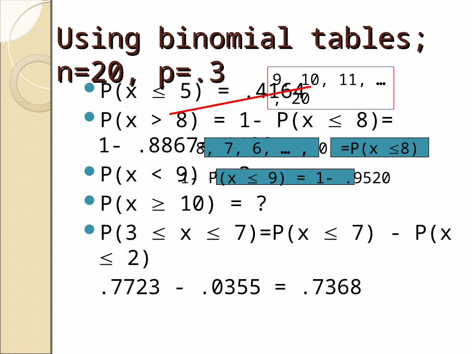
Using binomial tables; Using binomial tables; n=20, p=.3n=20, p=.3

P(x 5) = .4164P(x > 8) = 1- P(x 8)=

1- .8867=.1133P(x < 9) = ?P(x 10) = ?P(3 x 7)=P(x 7) - P(x 2)

.7723 - .0355 = .7368

9, 10, 11, … , 20

8, 7, 6, … , 0 =P(x 8)

1- P(x 9) = 1- .9520

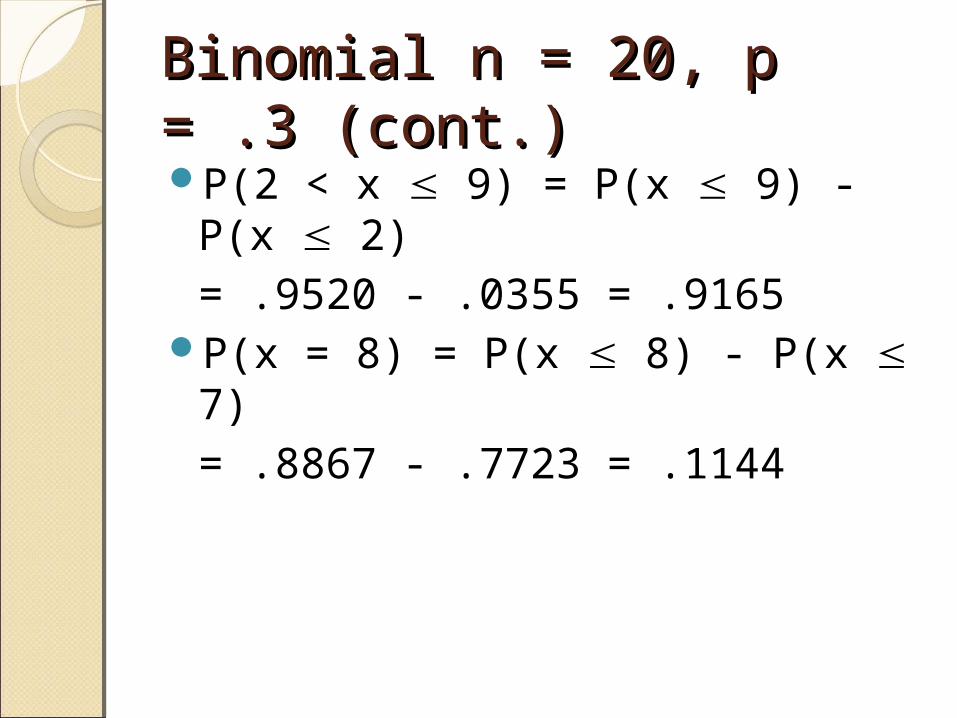
Binomial n = 20, p = .3 Binomial n = 20, p = .3 (cont.)(cont.)P(2 < x 9) = P(x 9) - P(x 2)

= .9520 - .0355 = .9165P(x = 8) = P(x 8) - P(x 7)

= .8867 - .7723 = .1144

Color blindness

The frequency of color blindness (dyschromatopsia) in the Caucasian American male population is estimated to be about 8%. We take a random sample of size 25 from this population.

We can model this situation with a B(n = 25, p = 0.08) distribution.

What is the probability that five individuals or fewer in the sample are color blind?

Use Excel’s “=BINOMDIST(number_s,trials,probability_s,cumulative)”

P(x ≤ 5) = BINOMDIST(5, 25, .08, 1) = 0.9877

What is the probability that more than five will be color blind?

P(x > 5) = 1 P(x ≤ 5) =1 0.9877 = 0.0123

What is the probability that exactly five will be color blind?

P(x = 5) = BINOMDIST(5, 25, .08, 0) = 0.0329

0%

5%

10%

15%

20%

25%

30%

0 2 4 6 8

10

12

14

16

18

20

22

24

Number of color blind individuals (x)

P(X

= x

)

Probability distribution and histogram for

the number of color blind individuals

among 25 Caucasian males.

x P(X = x) P(X <= x) 0 12.44% 12.44%1 27.04% 39.47%2 28.21% 67.68%3 18.81% 86.49%4 9.00% 95.49%5 3.29% 98.77%6 0.95% 99.72%7 0.23% 99.95%8 0.04% 99.99%9 0.01% 100.00%

10 0.00% 100.00%11 0.00% 100.00%12 0.00% 100.00%13 0.00% 100.00%14 0.00% 100.00%15 0.00% 100.00%16 0.00% 100.00%17 0.00% 100.00%18 0.00% 100.00%19 0.00% 100.00%20 0.00% 100.00%21 0.00% 100.00%22 0.00% 100.00%23 0.00% 100.00%24 0.00% 100.00%25 0.00% 100.00%

B(n = 25, p = 0.08)

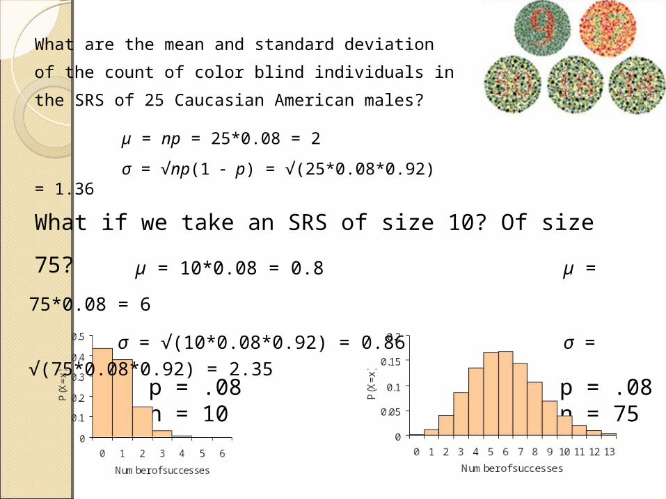
What are the mean and standard deviation of the

count of color blind individuals in the SRS of 25

Caucasian American males?

µ = np = 25*0.08 = 2

σ = √np(1 p) = √(25*0.08*0.92) = 1.36

p = .08n = 10

p = .08n = 75

µ = 10*0.08 = 0.8 µ = 75*0.08 = 6

σ = √(10*0.08*0.92) = 0.86 σ = √(75*0.08*0.92) = 2.35

What if we take an SRS of size 10? Of size 75?

Recall Free-throw Recall Free-throw questionquestion

Through 2/24/11 NC State’s free-throw percentage was 69.6% (146th in Div. 1).

If in the 2/26/11 game with GaTech, NCSU shoots 11 free-throws, what is the probability that:

1. NCSU makes exactly 8 free-throws?

2. NCSU makes at most 8 free throws?

3. NCSU makes at least 8 free-throws?

1. n=11; X=# of made free-throws; p=.696

p(8)= 11C8 (.696)8(.304)3

2. P(x ≤ 8)=.697

3. P(x ≥ 8)=1-P(x ≤7)=1-.4422 = .5578

Recall from beginning of Recall from beginning of Lecture Unit 4: Hardee’s vs Lecture Unit 4: Hardee’s vs

The ColonelThe ColonelOut of 100 taste-testers, 63

preferred Hardee’s fried chicken, 37 preferred KFC

Evidence that Hardee’s is better? A landslide?

What if there is no difference in the chicken? (p=1/2, flip a fair coin)

Is 63 heads out of 100 tosses that unusual?

Use binomial rv to analyzeUse binomial rv to analyze

n=100 taste testersx=# who prefer Hardees chickenp=probability a taste tester

chooses HardeesIf p=.5, P(x 63) = .0061 (since

the probability is so small, p is probably NOT .5; p is probably greater than .5, that is, Hardee’s chicken is probably better).

Recall: Mothers Recall: Mothers Identify NewbornsIdentify Newborns

After spending 1 hour with their newborns, blindfolded and nose-covered mothers were asked to choose their child from 3 sleeping babies by feeling the backs of the babies’ hands

22 of 32 women (69%) selected their own newborn

“far better than 33% one would expect…”Is it possible the mothers are guessing?Can we quantify “far better”?

Use binomial rv to Use binomial rv to analyzeanalyze

n=32 mothersx=# who correctly identify their own babyp= probability a mother chooses her own

babyIf p=.33, P(x 22)=.000044 (since the

probability is so small, p is probably NOT .33; p is probably greater than .33, that is, mothers are probably not guessing.