Binomial Distribution: Hypothesis Testing, Confidence Intervals (CI), and Reliability with Implementation in

S-PLUS

by Joseph C. Collins

ARL-TR-5214 June 2010 Approved for public release; distribution unlimited.

NOTICES

Disclaimers The findings in this report are not to be construed as an official Department of the Army position unless so designated by other authorized documents. Citation of manufacturer’s or trade names does not constitute an official endorsement or approval of the use thereof. Destroy this report when it is no longer needed. Do not return it to the originator.

Army Research Laboratory Aberdeen Proving Ground, MD 21005

ARL-TR-5214 June 2010

Binomial Distribution: Hypothesis Testing, Confidence Intervals (CI), and Reliability with Implementation in

S-PLUS

Joseph C. Collins Survivability/Lethality Analysis Directorate, ARL

Approved for public release; distribution unlimited.

ii

REPORT DOCUMENTATION PAGE Form Approved OMB No. 0704-0188

Public reporting burden for this collection of information is estimated to average 1 hour per response, including the time for reviewing instructions, searching existing data sources, gathering and maintaining the data needed, and completing and reviewing the collection information. Send comments regarding this burden estimate or any other aspect of this collection of information, including suggestions for reducing the burden, to Department of Defense, Washington Headquarters Services, Directorate for Information Operations and Reports (0704-0188), 1215 Jefferson Davis Highway, Suite 1204, Arlington, VA 22202-4302. Respondents should be aware that notwithstanding any other provision of law, no person shall be subject to any penalty for failing to comply with a collection of information if it does not display a currently valid OMB control number. PLEASE DO NOT RETURN YOUR FORM TO THE ABOVE ADDRESS. 1. REPORT DATE (DD-MM-YYYY)

June 2010 2. REPORT TYPE

Final 3. DATES COVERED (From - To)

January to June 2009 4. TITLE AND SUBTITLE

Binomial Distribution: Hypothesis Testing, Confidence Intervals (CI), and Reliability with Implementation in S-PLUS

5a. CONTRACT NUMBER

5b. GRANT NUMBER

5c. PROGRAM ELEMENT NUMBER

6. AUTHOR(S)

Joseph C. Collins 5d. PROJECT NUMBER

5e. TASK NUMBER

5f. WORK UNIT NUMBER

7. PERFORMING ORGANIZATION NAME(S) AND ADDRESS(ES)

U.S. Army Research Laboratory ATTN: RDRL-SLB-D Survivability/Lethality Analysis Directorate Aberdeen Proving Ground, MD 21005

8. PERFORMING ORGANIZATION REPORT NUMBER

ARL-TR-5214

9. SPONSORING/MONITORING AGENCY NAME(S) AND ADDRESS(ES)

10. SPONSOR/MONITOR'S ACRONYM(S)

11. SPONSOR/MONITOR'S REPORT NUMBER(S)

12. DISTRIBUTION/AVAILABILITY STATEMENT

Approved for public release; distribution unlimited.

13. SUPPLEMENTARY NOTES

14. ABSTRACT

System requirements can be expressed in terms of an upper (lower) limit on the probability of failure (success). Statistical analysis of such binary (0/1, success/failure, go/no-go) data typically requires point and interval estimation and inference or hypothesis tests on the associated event probability. For identical independent trials, the proportion observed serves as an estimate of the event rate. Based on the method of Clopper-Pearson (CP) and the likelihood ratio (LR) technique properties of the binomial distribution are used to derive interval estimates, which are in turn used in inference. An application is the determination of sample size and maximum permissible number of failures (nf) required to establish a specific reliability (probability of success) with given probability (confidence).

15. SUBJECT TERMS

binomial reliability, probability, statistics

16. SECURITY CLASSIFICATION OF: 17. LIMITATION

OF ABSTRACT

UU

18. NUMBER OF PAGES

43

19a. NAME OF RESPONSIBLE PERSON

Joseph C. Collins a. REPORT

Unclassified b. ABSTRACT

Unclassified c. THIS PAGE

Unclassified 19b. TELEPHONE NUMBER (Include area code)

(410) 278-6832 Standard Form 298 (Rev. 8/98) Prescribed by ANSI Std. Z39.18

iii

Contents

List of Figures v

List of Tables v

Summary 1

1. Binomial Distribution 3

1.1 Definitions and Properties ...............................................................................................3

1.2 Implementation Issue ......................................................................................................4

1.3 Beta Distribution .............................................................................................................5

2. Hypothesis Testing 8

2.1 One Sided Upper .............................................................................................................8

2.2 One Sided Lower .............................................................................................................9

2.3 Two Sided........................................................................................................................9

3. Confidence Intervals (CI) 10

3.1 Upper .............................................................................................................................10

3.2 Lower.............................................................................................................................10

3.3 Two Sided......................................................................................................................11

3.4 Implementation ..............................................................................................................11

3.5 Conservative Coverage..................................................................................................11

4. The LR Approach 14

4.1 Hypothesis Tests............................................................................................................15

4.2 Confidence Intervals......................................................................................................16

4.3 Implementation ..............................................................................................................17

5. Reliability 18

5.1 Reliability Tables ..........................................................................................................18

5.2 Sample Size ...................................................................................................................20

iv

6. References 22

Appendix A. S-PLUS Code 23

A.1 Library Functions ..........................................................................................................23

A.2 Upper-Tail Binomial Probabilities ................................................................................23

A.3 Binomial Parameter Confidence Interval: CP ...............................................................24

A.4 Binomial Reliability Table ............................................................................................24

A.5 Binomial Reliability Sample Size .................................................................................24

A.6 Binomial LR ..................................................................................................................25

A.7 Binomial LR cdf Table ..................................................................................................25

A.8 Binomial LR cdf Evaluation..........................................................................................26

A.9 Binomial LR Hypothesis Test .......................................................................................26

A.10 Binomial Parameter Confidence Interval: LR ...............................................................26

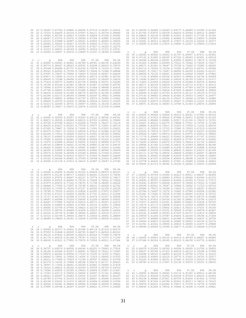
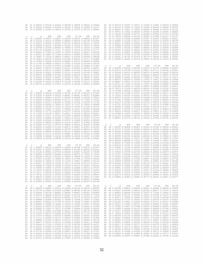
Appendix B. Reliability Table 29

List of Symbols, Abbreviations, and Acronyms 34 Distribution List 35

v

List of Figures

Figure 1. Binomial cdf and quantile function (qf) examples with continuous interpolation. .........7

Figure 2. Upper CI coverage. ........................................................................................................12

Figure 3. Lower CI coverage. .......................................................................................................13

Figure 4. Two-sided CP CI coverage. ...........................................................................................14

Figure 5. Two-sided LR CI coverage. ..........................................................................................17

Figure 6. Two-sided CI coverage comparison. .............................................................................17

List of Tables

Table 1. LR cdf. ............................................................................................................................16

Table 2. CP cdf. ............................................................................................................................16

vi

INTENTIONALLY LEFT BLANK.

1

Summary

The purpose of this report is to provide statisticians with the tools to solve certain reliability problems that arise in consultations with clients.

Statisticians often encounter clients seeking answers to questions such as, “I did an experiment 6 times with 3 successes and 3 failures, so the success rate is 50%, right?” A reasonable, useful, and informative response from the statistician would be, “yes, the estimate of success is 50%, but you can only state with 90% confidence that the true success rate lies between 15% and 85%. If you want to tighten that up, you need a larger sample.” The client asks, “how large?” and the conversation proceeds from there.

A client may pose a problem such as, “I need 90% confidence on 95% reliability. Can I do this with 10 runs?” The statistician can truthfully answer, no. You need 29 with no failures or 46 with 1 failure to assert 95% reliability with 90% confidence." The client may respond, “well, what can I get with 1 failure in 20?” and so the consultation continues.

In fact, the solutions to both of these problems exploit properties of the binomial distribution. System requirements can be expressed in terms of an upper (lower) limit on the probability of failure (success). Statistical analysis of such binary (0/1, success/failure, go/no-go) data typically requires point and interval estimation and inference or hypothesis tests on the associated event probability. For identical independent trials, the proportion observed serves as an estimate of the event rate. Based on the method of Clopper-Pearson (CP) and the likelihood ratio (LR) technique properties of the binomial distribution are used to derive interval estimates, which are in turn used in inference. An application is the determination of sample size and maximum permissible number of failures (nf) required to establish a specific reliability (probability of success) with given probability (confidence).

The statistician needs to address such issues and answer these questions in real time. This report provides the necessary technology expressed in the S-PLUS / S / R statistical computing environment language family, implementations of which are available as both commercial and free open-source software.

2

INTENTIONALLY LEFT BLANK.

3

1. Binomial Distribution

1.1 Definitions and Properties

The random variable 𝑋𝑋 is Bernoulli(𝑝𝑝), or 𝐵𝐵𝑝𝑝 , if 𝑋𝑋 ∈ {0,1} and Pr[𝑋𝑋 = 1] = 𝑝𝑝 = 1 − Pr[𝑋𝑋 =0]. The probability mass function, or discrete probability density function (pdf), is

𝑓𝑓𝑝𝑝(𝑥𝑥) = 𝑝𝑝𝑥𝑥(1 − 𝑝𝑝)1−𝑥𝑥 . (1)

The sum X of n independent and identically distributed (iid) Bp is Bernoulli(𝑛𝑛,𝑝𝑝), or 𝐵𝐵𝑛𝑛 ,𝑝𝑝 . Note that 𝐵𝐵𝑝𝑝 = 𝐵𝐵1,𝑝𝑝 . The binomial coefficient is (𝑛𝑛, 𝑘𝑘) = �𝑛𝑛𝑘𝑘� = 𝑛𝑛 !

𝑘𝑘!(𝑛𝑛−𝑘𝑘)! . Standard functions are

defined for 𝑘𝑘 ∈ {0,1,2, … ,𝑛𝑛}. The pdf is

𝑓𝑓𝑛𝑛 ,𝑝𝑝(𝑥𝑥) = 𝐶𝐶(𝑛𝑛, 𝑘𝑘)𝑝𝑝𝑥𝑥(1− 𝑝𝑝)1−𝑥𝑥 . (2)

The cumulative distribution function (cdf) is

𝐹𝐹𝑛𝑛 ,𝑝𝑝(𝑘𝑘) = Pr[𝑋𝑋 ≤ 𝑘𝑘] = �𝑓𝑓𝑛𝑛 ,𝑝𝑝(𝑗𝑗)𝑘𝑘

𝑗𝑗=0

(3)

with 𝐹𝐹𝑛𝑛 ,𝑝𝑝(𝑥𝑥) = 0 if 𝑥𝑥 ≤ 0, and 𝐹𝐹𝑛𝑛 ,𝑝𝑝(𝑥𝑥) = 1 if 𝑥𝑥 ≥ 𝑛𝑛, and right-continuous extension to ℝ, as is customary for discrete distributions. The quantile function (qf) is the usual unique left-continuous pseudo-inverse of the cdf,

𝑄𝑄𝑛𝑛 ,𝑝𝑝(𝑢𝑢) = inf � 𝑘𝑘: 𝐹𝐹𝑛𝑛 ,𝑝𝑝(𝑘𝑘) ≥ 𝑢𝑢 � (4)

It is also useful to have an upper-probability version of the cdf,

𝐺𝐺𝑛𝑛 ,𝑝𝑝(𝑘𝑘) = Pr[𝑋𝑋 ≥ 𝑘𝑘] = ∑ 𝑓𝑓𝑛𝑛 ,𝑝𝑝(𝑗𝑗)𝑛𝑛𝑗𝑗=𝑘𝑘 . (5)

So 𝐺𝐺𝑛𝑛 ,𝑝𝑝(𝑘𝑘) = 1 − 𝐹𝐹𝑛𝑛 ,𝑝𝑝(𝑘𝑘) and 𝐹𝐹𝑛𝑛 ,𝑝𝑝(𝑘𝑘) = 1 − 𝐺𝐺𝑛𝑛 ,𝑝𝑝(𝑘𝑘 + 1). Note that 𝐹𝐹𝑛𝑛 ,𝑝𝑝(𝑘𝑘) increases with k and decreases with n or p, and 𝐺𝐺𝑛𝑛 ,𝑝𝑝(𝑘𝑘) decreases with k and increases with n or p.

Moments are

E[𝑋𝑋𝑘𝑘] = �𝑗𝑗𝑘𝑘𝑓𝑓𝑛𝑛 ,𝑝𝑝(𝑗𝑗) 𝑛𝑛

𝑗𝑗=0

(6)

So E[𝑋𝑋] = 𝑛𝑛𝑝𝑝, and E[𝑋𝑋2] = 𝑛𝑛𝑝𝑝(1 − 𝑝𝑝) + 𝑛𝑛2𝑝𝑝2, and Var[X] = 𝑛𝑛𝑝𝑝(1 − 𝑝𝑝).

4

The log-likelihood function is

ℒ = ��log𝐶𝐶(𝑛𝑛, 𝑗𝑗) + 𝑋𝑋𝑗𝑗 log 𝑝𝑝 + �𝑛𝑛 − 𝑋𝑋𝑗𝑗 � log(1 − 𝑝𝑝)�𝑛𝑛

𝑗𝑗=0

= �� log𝐶𝐶(𝑛𝑛, 𝑗𝑗)𝑛𝑛

𝑗𝑗=0

�+ 𝑘𝑘 log𝑝𝑝 + (𝑛𝑛 − 𝑘𝑘) log(1 − 𝑝𝑝) .

(7)

The maximum likelihood estimator (MLE) of p is 𝑘𝑘 𝑛𝑛⁄ .

1.2 Implementation Issue

Reasonable algorithms for 𝐹𝐹𝑛𝑛 ,𝑝𝑝(𝑘𝑘) return the appropriate values for large n and small k but succumb to numeric underflow for large k.

For example, since 𝐹𝐹𝑛𝑛 ,𝑝𝑝(0) = (1 − 𝑝𝑝)𝑛𝑛 and 𝐹𝐹𝑛𝑛 ,𝑝𝑝(𝑛𝑛 − 1) = 1 − 𝑝𝑝𝑛𝑛 , set 𝑛𝑛 = 100 and 𝑝𝑝 = 0.6 to get

𝐹𝐹100,0.6(0) = (1 − 0.6)100 = 0.4100 ≅ 1.6 × 10−40 (8)

and

𝐹𝐹100,0.6(99) = 1 − 0.6100 ≅ 1 − 6.5 × 10−23. (9)

But with standard double precision resolution of about 16 decimal places, the result is 𝐹𝐹100,0.6(99) = 1 exactly. The cure for lower tail probabilities too close to 1 is to use upper tail probabilities, which will be close to 0, and work with G instead of F, since 𝐺𝐺𝑛𝑛 ,𝑝𝑝(𝑛𝑛) = 𝑝𝑝𝑛𝑛 = 1 −𝐹𝐹𝑛𝑛 ,𝑝𝑝(𝑛𝑛 − 1), and so

𝐺𝐺100,0.6(100) = 0.6100 = 1 − 𝐹𝐹100,0.6(99) = 1 − (1 − 0.6)100 ≅ 6.5 × 10−23 . (10)

But naïve use of 𝐺𝐺𝑛𝑛 ,𝑝𝑝(𝑘𝑘) = 1 − 𝐹𝐹𝑛𝑛 ,𝑝𝑝(𝑘𝑘 − 1) directly will of course give 𝐺𝐺100,0.6(100) = 0. To obtain a useful representation of 𝐺𝐺(𝑘𝑘) with k large in terms of an accurate algorithm for 𝐹𝐹(𝑘𝑘) with k small, let 𝑋𝑋 ~𝐵𝐵𝑛𝑛 ,𝑝𝑝 and 𝑊𝑊 = 𝑛𝑛 − 𝑋𝑋. Note that 𝐹𝐹𝑊𝑊(𝑘𝑘) = Pr[ 𝑊𝑊 ≤ 𝑘𝑘] = Pr[ 𝑛𝑛 − 𝑋𝑋 ≤ 𝑘𝑘] =Pr[𝑋𝑋 ≥ 𝑛𝑛 − 𝑘𝑘] = 1 − Pr[𝑋𝑋 < 𝑛𝑛 − 𝑘𝑘] = 1 − Pr[𝑋𝑋 ≤ 𝑛𝑛 − 𝑘𝑘 − 1] = 1 − 𝐹𝐹𝑋𝑋(𝑛𝑛 − 𝑘𝑘 − 1) . Then 𝐺𝐺𝑋𝑋(𝑘𝑘) = 1 − 𝐹𝐹𝑋𝑋(𝑘𝑘 − 1) = 1 − 𝐹𝐹𝑋𝑋(𝑛𝑛 − (𝑛𝑛 − 𝑘𝑘) − 1) = 𝐹𝐹𝑊𝑊(𝑛𝑛 − 𝑘𝑘), so

𝐺𝐺𝑛𝑛 ,𝑝𝑝(𝑘𝑘) = 𝑃𝑃𝑃𝑃�𝐵𝐵𝑛𝑛 ,𝑝𝑝 ≤ 𝑘𝑘� = Pr�𝐵𝐵𝑛𝑛 ,1−𝑝𝑝 ≤ 𝑛𝑛 − 𝑘𝑘� = 𝐹𝐹𝑛𝑛 ,1−𝑝𝑝(𝑛𝑛 − 𝑘𝑘). (11)

This gives 𝐺𝐺100,0.6(100) = 𝐹𝐹100,0.4(0) = (1 − 0.4)100 = 0.6100 ≅ 6.5 × 10−23 as required.

5

1.3 Beta Distribution

The Gamma function, which has Γ(𝑛𝑛) = (𝑛𝑛 − 1)! for n = 1,2,3,…, is given by

Γ(𝑧𝑧) = � 𝑢𝑢𝑧𝑧−1𝑒𝑒−𝑢𝑢𝑑𝑑𝑢𝑢∞

0. (12)

The Beta function, which has 𝐵𝐵(𝑛𝑛,𝑘𝑘) = (𝑛𝑛 − 1)! (𝑘𝑘 − 1)!/(𝑛𝑛 + 𝑘𝑘 − 1)! on positive integers, is

𝐵𝐵(𝑎𝑎, 𝑏𝑏) =Γ(𝑎𝑎)Γ(𝑏𝑏)Γ(𝑎𝑎 + 𝑏𝑏) = � 𝑥𝑥𝑎𝑎−1(1 − 𝑥𝑥)𝑏𝑏−1𝑑𝑑𝑥𝑥

1

0. (13)

The Beta (𝑎𝑎, 𝑏𝑏) distribution on [0,1], with 𝑎𝑎 > 0 and 𝑏𝑏 > 0, has pdf and cdf

𝑓𝑓Beta (𝑎𝑎 ,𝑏𝑏)(𝑥𝑥) =1

𝐵𝐵(𝑎𝑎, 𝑏𝑏) 𝑥𝑥𝑎𝑎−1(1 − 𝑥𝑥)𝑏𝑏−1

𝐹𝐹Beta (𝑎𝑎 ,𝑏𝑏)(𝑥𝑥) = � 𝑓𝑓Beta (𝑎𝑎 ,𝑏𝑏)(𝑢𝑢) 𝑑𝑑𝑢𝑢𝑥𝑥

0.

(14)

The Binomial and Beta cdfs are related by 𝐹𝐹𝑛𝑛 ,𝑝𝑝(𝑘𝑘 − 1) = 𝐹𝐹Beta (𝑛𝑛−𝑘𝑘+1,𝑘𝑘)(1 − 𝑝𝑝), so

𝐹𝐹𝑛𝑛 ,𝑝𝑝(𝑘𝑘) = 𝐹𝐹Beta (𝑛𝑛−𝑘𝑘 ,𝑘𝑘+1)(1 − 𝑝𝑝), or

𝐹𝐹𝑛𝑛−𝑘𝑘+1,1−𝑝𝑝(𝑘𝑘 − 1) = 𝐹𝐹Beta (𝑛𝑛 ,𝑘𝑘)(𝑝𝑝) (15)

and also

𝐺𝐺𝑛𝑛 ,𝑝𝑝(𝑘𝑘) = 𝐹𝐹Beta (𝑘𝑘 ,𝑛𝑛−𝑘𝑘+1)(𝑝𝑝), or

𝐺𝐺𝑛𝑛−𝑘𝑘+1,𝑝𝑝(𝑘𝑘) = 𝐹𝐹Beta (𝑛𝑛 ,𝑘𝑘)(𝑝𝑝). (16)

To show 𝐹𝐹𝑛𝑛 ,𝑝𝑝(𝑘𝑘 − 1) = 𝐹𝐹Beta (𝑛𝑛−𝑘𝑘+1,𝑘𝑘)(1 − 𝑝𝑝), first note that 𝐵𝐵(𝑛𝑛 − 𝑘𝑘 + 1, 𝑘𝑘) = (𝑛𝑛 − 𝑘𝑘)! (𝑘𝑘 −1)!/𝑛𝑛!, and also 𝐹𝐹Beta (𝑛𝑛 ,1) (1 − 𝑝𝑝) = 𝑛𝑛 ∫ 𝑥𝑥𝑛𝑛−1𝑑𝑑𝑥𝑥 = (1 − 𝑝𝑝)𝑛𝑛 = 𝑓𝑓𝑛𝑛 ,𝑝𝑝(0)1

0 . Now, integrating by parts,

6

𝐹𝐹Beta (𝑛𝑛−𝑘𝑘+1,𝑘𝑘)(1− 𝑝𝑝) =𝑛𝑛!

(𝑛𝑛 − 𝑘𝑘)! (𝑘𝑘 − 𝑛𝑛)!� 𝑥𝑥𝑛𝑛−𝑘𝑘(1− 𝑥𝑥)𝑘𝑘−1𝑑𝑑𝑥𝑥

1−𝑝𝑝

0

=𝑛𝑛!

(𝑛𝑛 − 𝑘𝑘)! (𝑘𝑘 − 𝑛𝑛)!��𝑥𝑥𝑛𝑛−𝑘𝑘(1 − 𝑥𝑥)𝑘𝑘−1

𝑛𝑛 − 𝑘𝑘 + 1�

0

1−𝑝𝑝

+ �(𝑘𝑘 − 1)𝑥𝑥𝑛𝑛−𝑘𝑘+1(1 − 𝑥𝑥)𝑘𝑘−2

𝑛𝑛 − 𝑘𝑘 + 1

1−𝑝𝑝

0�

=𝑛𝑛!𝑝𝑝𝑘𝑘−1(1 − 𝑝𝑝)𝑛𝑛−𝑘𝑘+1

(𝑛𝑛 − 𝑘𝑘 + 1)! (𝑘𝑘 − 1)!+

𝑛𝑛!(𝑘𝑘 − 2)! (𝑛𝑛 − 𝑘𝑘 + 1)!

� 𝑥𝑥𝑛𝑛−𝑘𝑘+1(1 − 𝑥𝑥)𝑘𝑘−2𝑑𝑑𝑥𝑥1−𝑝𝑝

0

= 𝑓𝑓𝑛𝑛 ,𝑝𝑝(𝑘𝑘 − 1) +1

𝐵𝐵(𝑛𝑛 − 𝑘𝑘 + 2,𝑘𝑘 − 1)� 𝑥𝑥𝑛𝑛−𝑘𝑘+1(1− 𝑥𝑥)𝑘𝑘−2𝑑𝑑𝑥𝑥1−𝑝𝑝

0

= 𝑓𝑓𝑛𝑛 ,𝑝𝑝(𝑘𝑘 − 1) + 𝐹𝐹Beta (𝑛𝑛−𝑘𝑘+2,𝑘𝑘−1)(1 − 𝑝𝑝)

= 𝑓𝑓𝑛𝑛 ,𝑝𝑝(𝑘𝑘 − 1) + ⋯+ 𝑓𝑓𝑛𝑛 ,𝑝𝑝(1) + 𝐹𝐹Beta (𝑛𝑛 ,1) (1− 𝑝𝑝)

= 𝑓𝑓𝑛𝑛 ,𝑝𝑝(𝑘𝑘 − 1) + ⋯+ 𝑓𝑓𝑛𝑛 ,𝑝𝑝(1) + 𝑓𝑓𝑛𝑛 ,𝑝𝑝(0)

= 𝐹𝐹𝑛𝑛 ,𝑝𝑝(𝑘𝑘 − 1). (17)

See, for example, Stuart (1).

In fact, the function

𝐹𝐹(𝑥𝑥) = �

0, 𝑥𝑥 ≤ −1

𝐹𝐹Beta (𝑛𝑛−𝑥𝑥+1,𝑥𝑥)(1− 𝑝𝑝), −1 < 𝑥𝑥 < 𝑛𝑛

1, 𝑛𝑛 ≤ 𝑥𝑥

� (18)

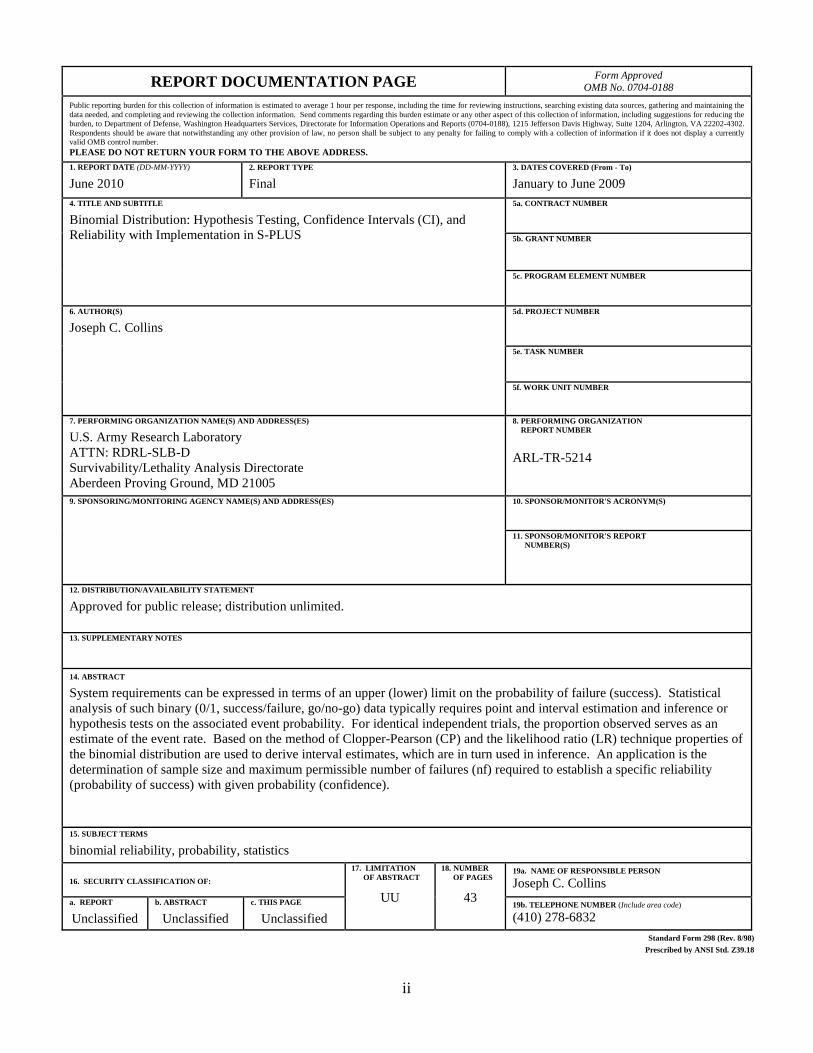
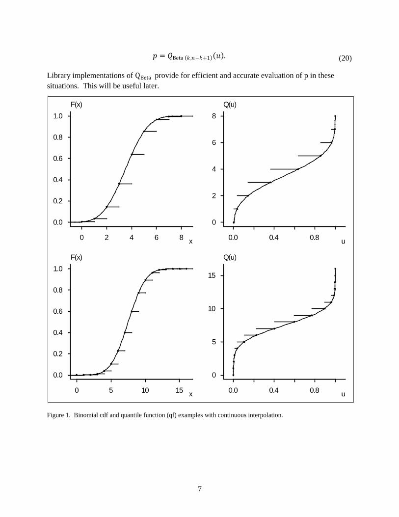
is a continuous cdf on [−1,𝑛𝑛], and 𝐹𝐹(𝑘𝑘) = 𝐹𝐹𝑛𝑛 ,𝑝𝑝(𝑘𝑘) for 𝑘𝑘 = 0,1,2, … ,𝑛𝑛. So F serves as a continuous version, or interpolation, of 𝐹𝐹𝑛𝑛 ,𝑝𝑝 , which is sometimes useful. The corresponding quantile function 𝑄𝑄(𝑢𝑢) = 𝐹𝐹−1(𝑢𝑢) is not related to 𝑄𝑄Beta , but can be obtained by solving 𝐹𝐹(𝑥𝑥) =𝑢𝑢 numerically to get 𝑥𝑥 = 𝑄𝑄(𝑢𝑢). See figure 1.

Note that 𝑄𝑄Beta does provide the solution p of 𝑢𝑢 = 𝐹𝐹𝑛𝑛 ,𝑝𝑝(𝑘𝑘). Since 𝑢𝑢 = 𝐹𝐹𝑛𝑛 ,𝑝𝑝(𝑘𝑘) = 𝐹𝐹Beta (𝑛𝑛−𝑘𝑘 ,𝑘𝑘+1)(1 − 𝑝𝑝), and so 𝑄𝑄Beta (𝑛𝑛−𝑘𝑘 ,𝑘𝑘+1)(𝑢𝑢) = 1 − 𝑝𝑝, observe that

𝑝𝑝 = 1 − 𝑄𝑄Beta (𝑛𝑛−𝑘𝑘 ,𝑘𝑘+1)(𝑢𝑢). (19)

Likewise for 𝑢𝑢 = 𝐺𝐺(𝑛𝑛 ,𝑝𝑝)(𝑘𝑘). Since 𝑢𝑢 = 𝐺𝐺𝑛𝑛 ,𝑝𝑝(𝑘𝑘) = 𝐹𝐹Beta (𝑘𝑘 ,𝑛𝑛−𝑘𝑘+1)(𝑝𝑝) and so 𝑄𝑄Beta (𝑘𝑘 ,𝑛𝑛−𝑘𝑘+1)(𝑢𝑢) =𝑝𝑝, it follows that

7

𝑝𝑝 = 𝑄𝑄Beta (𝑘𝑘 ,𝑛𝑛−𝑘𝑘+1)(𝑢𝑢). (20)

Library implementations of QBeta provide for efficient and accurate evaluation of p in these situations. This will be useful later.

Figure 1. Binomial cdf and quantile function (qf) examples with continuous interpolation.

0 2 4 6 8

0.0

0.2

0.4

0.6

0.8

1.0

x

F(x)

0.0 0.4 0.8

0

2

4

6

8

u

Q(u)

0 5 10 15

0.0

0.2

0.4

0.6

0.8

1.0

x

F(x)

0.0 0.4 0.8

0

5

10

15

u

Q(u)

8

2. Hypothesis Testing

Tests of size 𝛾𝛾 and Type I error probability 𝛼𝛼 = 1 − 𝛾𝛾 for

𝐻𝐻0:𝑝𝑝 = 𝑝𝑝𝑜𝑜 (21)

are based on data X. Here 𝛼𝛼 is the null rejection probability, or probability of rejecting 𝐻𝐻0 when it is true. See Mood (2) or Stuart (3) for an explanation.

2.1 One Sided Upper

The one-sided alternative

𝐻𝐻1:𝑝𝑝 < 𝑝𝑝𝑜𝑜 (22)

provides an upper limit for p upon rejection of 𝐻𝐻0. The critical value is 𝑘𝑘𝑈𝑈 , and the decision rule is to reject 𝐻𝐻0 if 𝑋𝑋 ≤ 𝑘𝑘𝑈𝑈 where Pr[𝑋𝑋 ≤ 𝑘𝑘𝑈𝑈 | 𝐻𝐻0] = 𝛼𝛼. Since X is discrete, take

𝑘𝑘𝑈𝑈 = sup { 𝑘𝑘 | Pr[𝑋𝑋 ≤ 𝑘𝑘 |𝐻𝐻0] ≤ 𝛼𝛼 } = sup �𝑘𝑘 � 𝐹𝐹𝑛𝑛 ,𝑝𝑝𝑜𝑜(𝑘𝑘) ≤ 𝛼𝛼�. (23)

The rejection region is 𝐼𝐼1 = { 0, … ,𝑘𝑘𝑈𝑈 }, and the non-rejection region is 𝐼𝐼0 = { 𝑘𝑘𝑈𝑈 + 1, … ,𝑛𝑛 }. Equivalently, the p-value for the test is 𝑝𝑝𝑋𝑋 = 𝐹𝐹𝑛𝑛 ,𝑝𝑝𝑜𝑜(𝑋𝑋), and the rule is to reject 𝐻𝐻0 if 𝑝𝑝𝑋𝑋 ≤ 𝛼𝛼. For example, let 𝑝𝑝𝑜𝑜 = 0.3 and 𝛼𝛼 = 0.1 with 𝑛𝑛 = 100. Since 𝐹𝐹100,0.3(23) = 0.0755 and 𝐹𝐹100,0.3(24) = 0.114, it follows that 𝑘𝑘𝑈𝑈 = 23. These are also the p-values, 𝑝𝑝23 = 0.0755 and 𝑝𝑝24 = 0.114. The true value of 𝛼𝛼 for this test is 0.0755.

For example, it is possible for the test to degenerate due to insufficient sample size. Consider 𝑝𝑝𝑜𝑜 = 0.03 and 𝛼𝛼 = 0.01 with 𝑛𝑛 = 100. Since 𝐹𝐹100,0.03(0) = 0.0476, it follows that 𝐹𝐹100,0.03(𝑘𝑘) > 𝛼𝛼 for all k, and so 𝐼𝐼1 = ∅, and 𝐼𝐼0 = {0, … ,𝑛𝑛}, and rejection never occurs. The true value of 𝛼𝛼 for this test is .

But 𝐹𝐹151,0.03(0) = 0.0101 and 𝐹𝐹152,0.03(0) = 0.00976, so 𝑛𝑛 > 151 is required for a non-degenerate test. With 𝑛𝑛 = 152, since 𝐹𝐹152,0.03(1) = 0.0556, it follows that 𝑘𝑘𝑈𝑈 = 0. Then if 𝑋𝑋 = 0 the decision is to reject 𝐻𝐻0 and conclude that 𝑝𝑝 < 0.03 with probability ≥ 0.99. If 𝑋𝑋 > 0 there is no indication that 𝑝𝑝 < 0.03. The true value of 𝛼𝛼 for this test is 0.00976.

Let 𝑝𝑝𝑜𝑜 = 1 2⁄ and 𝛼𝛼 = 7 128⁄ with 𝑛𝑛 = 10. Note that 𝐹𝐹10,1 2⁄ (2) = 7 128⁄ = 𝛼𝛼. It follows that 𝑘𝑘𝑈𝑈 = 2 and 𝑝𝑝𝑋𝑋 ≤ 𝛼𝛼 when 𝑋𝑋 ≤ 2, in which case 𝐻𝐻0 is rejected. The true value of 𝛼𝛼 for this test is exactly 7 128⁄ .

9

2.2 One Sided Lower

The one-sided alternative

𝐻𝐻1: 𝑝𝑝 > 𝑝𝑝𝑜𝑜 (24)

provides a lower limit for p upon rejection of 𝐻𝐻0. The critical value is 𝑘𝑘𝐿𝐿, and one rejects 𝐻𝐻0 if 𝑋𝑋 ≥ 𝑘𝑘𝐿𝐿 where Pr[𝑋𝑋 ≥ 𝑘𝑘𝐿𝐿|𝐻𝐻0] = 𝛼𝛼. Since X is discrete, take

𝑘𝑘𝐿𝐿 = 𝑖𝑖𝑛𝑛𝑓𝑓{𝑘𝑘|𝑃𝑃𝑃𝑃[𝑋𝑋 ≥ 𝑘𝑘 |𝐻𝐻0] ≤ 𝛼𝛼} = inf � 𝑘𝑘 � 𝐺𝐺𝑛𝑛 ,𝑝𝑝𝑜𝑜 (𝑘𝑘) ≤ 𝛼𝛼�. (25)

The rejection region is 𝐼𝐼1 = {𝑘𝑘𝐿𝐿 , … , 𝑛𝑛}, and the non-rejection region is 𝐼𝐼0 = {0, … ,𝑘𝑘𝐿𝐿 − 1}. Equivalently, the p-value for the test is 𝑝𝑝𝑋𝑋 = 𝐺𝐺𝑛𝑛 ,𝑝𝑝𝑜𝑜 (𝑋𝑋), and one rejects 𝐻𝐻0 if 𝑝𝑝𝑋𝑋 ≤ 𝛼𝛼.

For example, let 𝑝𝑝𝑜𝑜 = 0.3 and 𝛼𝛼 = 0.1 with 𝑛𝑛 = 100. Since 𝐺𝐺100,0.3(36) = 0.116 and 𝐺𝐺100,0.3(37) = 0.0799, it follows that 𝑘𝑘𝐿𝐿 = 37. These are also the p-values, 𝑝𝑝36 = 0.116 and 𝑝𝑝37 = 0.0799.

2.3 Two Sided

The two-sided alternative

𝐻𝐻1:𝑝𝑝 ≠ 𝑝𝑝𝑜𝑜 (26)

provides upper and lower limits for p upon rejection of 𝐻𝐻0. The critical values are 𝑘𝑘𝑈𝑈 and 𝑘𝑘𝐿𝐿, and one rejects 𝐻𝐻0 if 𝑋𝑋 ≤ 𝑘𝑘𝑈𝑈 or 𝑋𝑋 ≥ 𝑘𝑘𝑈𝑈 where Pr[𝑋𝑋 ≤ 𝑘𝑘𝑈𝑈 𝑜𝑜𝑃𝑃 𝑋𝑋 ≥ 𝑘𝑘𝐿𝐿 |𝐻𝐻0 ] = 𝛼𝛼. For symmetry, set Pr[𝑋𝑋 ≤ 𝑘𝑘𝑈𝑈 |𝐻𝐻0] = Pr[𝑋𝑋 ≥ 𝑘𝑘𝐿𝐿| 𝐻𝐻0] = 𝛼𝛼 2⁄ . Since X is discrete, take

𝑘𝑘𝑈𝑈 = sup{𝑘𝑘 | Pr[𝑋𝑋 ≤ 𝑘𝑘 |𝐻𝐻0] ≤ 𝛼𝛼 2⁄ } = sup�𝑘𝑘 � 𝐹𝐹𝑛𝑛 ,𝑝𝑝𝑜𝑜(𝑘𝑘) ≤ 𝛼𝛼 2⁄ � 𝑘𝑘𝐿𝐿 = inf{𝑘𝑘| Pr[𝑋𝑋 ≥ 𝑘𝑘 |𝐻𝐻0] ≤ 𝛼𝛼 2⁄ } = inf�𝑘𝑘 � 𝐺𝐺𝑛𝑛 ,𝑝𝑝𝑜𝑜 (𝑘𝑘) ≤ 𝛼𝛼 2⁄ � (27)

The rejection region is 𝐼𝐼1 = {0, … ,𝑘𝑘𝑈𝑈} ∪ {𝑘𝑘𝐿𝐿 , … ,𝑛𝑛}, and the non-rejection region is 𝐼𝐼0 = {𝑘𝑘𝑈𝑈 +1, … , 𝑘𝑘𝐿𝐿 − 1}. Equivalently, the p-value for the test is 𝑝𝑝𝑋𝑋 = 2 min �𝐹𝐹𝑛𝑛 ,𝑝𝑝𝑜𝑜 (𝑋𝑋),𝐺𝐺𝑛𝑛 ,𝑝𝑝𝑜𝑜 (𝑋𝑋)�. One rejects 𝐻𝐻0 if 𝑝𝑝𝑋𝑋 ≤ 𝛼𝛼.

For example, let 𝑝𝑝𝑜𝑜 = 0.3 and 𝛼𝛼 = 0.1 with 𝑛𝑛 = 100. Since 𝐹𝐹100,0.3(22) = 0.0479 and 𝐹𝐹100,0.3(23) = 0.0755, it follows that 𝑘𝑘𝑈𝑈 = 22. Since 𝐺𝐺100,0.3(38) = 0.0530 and 𝐺𝐺100,0.3(39) = 0.0340, it follows that 𝑘𝑘𝐿𝐿 = 39. Note that 𝐺𝐺100,0.3(22) = 0.971, 𝐺𝐺100,0.3(23) =0.952, 𝐹𝐹100,0.3(38) = 0.966, and 𝐹𝐹100,0.3(39) = 0.979. So the p-values are 𝑝𝑝22 = 0.0957, 𝑝𝑝23 = 0.151, 𝑝𝑝38 = 0.106, and 𝑝𝑝39 = 0.0680.

10

3. Confidence Intervals (CI)

The point estimate of p is of course 𝑋𝑋 𝑛𝑛⁄ . CIs on p are obtained by pivoting or inverting hypothesis test critical regions as follows. See Clopper and Pearson (4).

3.1 Upper

Let 𝐼𝐼1 be the set of 𝑝𝑝𝑜𝑜 for which 𝐻𝐻0 would be rejected in favor of 𝐻𝐻1:𝑝𝑝 < 𝑝𝑝𝑜𝑜with Type I error 𝛼𝛼, so 𝐼𝐼1 = { 𝑝𝑝 |𝐹𝐹𝑛𝑛 ,𝑝𝑝(𝑋𝑋) ≤ 𝛼𝛼 } = [𝑝𝑝𝑈𝑈 , 1] where

𝛼𝛼 = 𝐹𝐹𝑛𝑛 ,𝑝𝑝𝑈𝑈 (𝑋𝑋) = 𝐹𝐹Beta (𝑛𝑛−𝑋𝑋,𝑋𝑋+1)(1 − 𝑝𝑝𝑈𝑈), (28)

so 𝑝𝑝𝑈𝑈 can be expressed by equation 19 as a Beta distribution quantile

𝑝𝑝𝑈𝑈 = 1 − 𝑄𝑄Beta (𝑛𝑛−𝑋𝑋,𝑋𝑋+1)(𝛼𝛼). (29)

Null rejection occurs with probability 𝛼𝛼, so the non-rejection region

𝐼𝐼0 = [0, 𝑝𝑝𝑈𝑈) = { 𝑝𝑝 |𝐹𝐹𝑛𝑛 ,𝑝𝑝(𝑋𝑋) > 𝛼𝛼 } (30)

is a 100𝛾𝛾% upper CI on p, and 𝑝𝑝𝑈𝑈 is an upper confidence limit on p. To reject 𝐻𝐻0 when 𝑝𝑝 ∈ 𝐼𝐼1 = [𝑝𝑝𝑈𝑈 , 1] is precisely the p-value decision rule in section 0.

3.2 Lower

Let 𝐼𝐼1be the set of 𝑝𝑝𝑜𝑜 for which 𝐻𝐻0 would be rejected in favor of 𝐻𝐻1:𝑝𝑝 > 𝑝𝑝𝑜𝑜with Type I error 𝛼𝛼, so 𝐼𝐼1 = { 𝑝𝑝 |𝐺𝐺𝑛𝑛 ,𝑝𝑝(𝑋𝑋) ≤ 𝛼𝛼 } = [0,𝑝𝑝𝐿𝐿] where

𝛼𝛼 = 𝐺𝐺𝑛𝑛 ,𝑝𝑝𝐿𝐿(𝑋𝑋) = 𝐹𝐹Beta (𝑋𝑋,𝑛𝑛−𝑋𝑋+1)(𝑝𝑝𝐿𝐿), (31)

so 𝑝𝑝𝐿𝐿 can be expressed by equation (20) as a Beta distribution quantile

𝑝𝑝𝐿𝐿 = 𝑄𝑄Beta (𝑋𝑋 ,𝑛𝑛−𝑋𝑋+1)(𝛼𝛼).. (32)

Null rejection occurs with probability 𝛼𝛼, so the non-rejection region

𝐼𝐼0 = (𝑝𝑝𝐿𝐿 , 1] = { 𝑝𝑝 |𝐺𝐺𝑛𝑛 ,𝑝𝑝(𝑋𝑋) > 𝛼𝛼 } (33)

is a 100𝛾𝛾% lower CI on p, and 𝑝𝑝𝐿𝐿 is a lower confidence limit on p. To reject 𝐻𝐻0 when 𝑝𝑝 ∈ 𝐼𝐼1 =[1, 𝑝𝑝𝐿𝐿] is precisely the p-value decision rule in section 2.2.

11

3.3 Two Sided

Let 𝐼𝐼1be the set of 𝑝𝑝𝑜𝑜 for which 𝐻𝐻0 would be rejected in favor of 𝐻𝐻1:𝑝𝑝 ≠ 𝑝𝑝𝑜𝑜 with Type I error 𝛼𝛼, so 𝐼𝐼1 = { 𝑝𝑝 | 𝐺𝐺𝑛𝑛 ,𝑝𝑝(𝑋𝑋) ≤ 𝛼𝛼 2} ∪ { 𝑝𝑝 |𝐹𝐹𝑛𝑛 ,𝑝𝑝(𝑋𝑋) ≤ 𝛼𝛼 2⁄ } = [0,𝑝𝑝𝐿𝐿] ∪ [𝑝𝑝𝑈𝑈 , 1]⁄ where

𝐺𝐺𝑛𝑛 ,𝑝𝑝𝐿𝐿(𝑋𝑋) = 𝐹𝐹𝑛𝑛 ,𝑝𝑝𝑈𝑈 (𝑋𝑋) = 𝛼𝛼 2⁄ . (34)

Then 𝑝𝑝𝐿𝐿 and 𝑝𝑝𝑈𝑈 can be expressed by equations 19 and 20 as Beta distributions quantiles

𝑝𝑝𝐿𝐿 = 𝑄𝑄Beta (𝑋𝑋 ,𝑛𝑛−𝑋𝑋+1) (𝛼𝛼 2⁄ )

𝑝𝑝𝑈𝑈 = 1 − 𝑄𝑄Beta (𝑛𝑛−𝑋𝑋,𝑋𝑋+1) (𝛼𝛼 2⁄ ). (35)

Null rejection occurs with probability 𝛼𝛼, so the non-rejection region

𝐼𝐼0 = (𝑝𝑝𝐿𝐿 ,𝑝𝑝𝑈𝑈) = { 𝑝𝑝 |𝐺𝐺𝑛𝑛 ,𝑝𝑝(𝑋𝑋) > 𝛼𝛼 2⁄ } ∩ { 𝑝𝑝 |𝐹𝐹𝑛𝑛 ,𝑝𝑝(𝑋𝑋) > 𝛼𝛼 2⁄ } (36)

is a 100𝛾𝛾% two-sided CI on p. To reject 𝐻𝐻0 when 𝑝𝑝𝑜𝑜 ∈ [0, 𝑝𝑝𝐿𝐿] ∪ [𝑝𝑝𝑈𝑈 , 1] is precisely the p-value decision rule of section 2.3.

3.4 Implementation

Code listings are in appendix A.

The function bino.ci(n,r,g,type) uses equations 29, 32, or 35 to give the required CI. The arguments of bino.ci are the number of trials n, the number of successes r, confidence interval size g which should be between 0.5 and 1.0, and an integer type which can be 0, 1, or 2 to request a lower CI (𝐿𝐿, 1], upper CI [0,𝑈𝑈), or 2-sided CI (𝐿𝐿,𝑈𝑈), respectively.

The return value from bino.ci is a named list holding the number of trials $n, number of successes $r, lower limit $L, parameter estimate $p.hat, upper limit $U, and confidence interval vector $I. For example,

bino.ci(n=100, r=30, g=0.9, type=2)

returns $n: 100 $r: 30 $L: 0.22492 $p.hat: 0.3 $U: 0.38422 $I: 0.22492 0.38422

since Pr�𝐵𝐵100,0.22492 ≥ 30� = Pr�𝐵𝐵100,0.38422 ≤ 30� = 0.05.

3.5 Conservative Coverage

Coverage is the probability that a confidence interval captures the true parameter value.

12

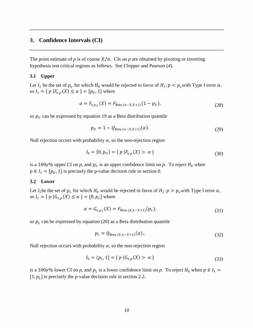
Considering that 𝑝𝑝𝑈𝑈(𝑋𝑋) is random, and [0, 𝑝𝑝𝑈𝑈(𝑋𝑋)) is a 100𝛾𝛾% CI on p, one expects that 𝐶𝐶𝑈𝑈(𝑝𝑝) = Pr[𝑝𝑝 < 𝑝𝑝𝑈𝑈(𝑋𝑋)] = E �𝐼𝐼�0,𝑝𝑝𝑈𝑈 (𝑋𝑋)�(𝑝𝑝)� ≥ 𝛾𝛾. This coverage probability is

𝐶𝐶𝑈𝑈(𝑝𝑝) = ∑ 𝑃𝑃𝑃𝑃[𝑋𝑋 = 𝑘𝑘] ∙ 𝐼𝐼�0,𝑝𝑝𝑈𝑈 (𝑋𝑋)�(𝑝𝑝) = ∑ 𝑓𝑓𝑛𝑛 ,𝑝𝑝(𝑘𝑘)𝑝𝑝<𝑝𝑝𝑈𝑈 (𝑘𝑘)𝑛𝑛𝑘𝑘=0 . (37)

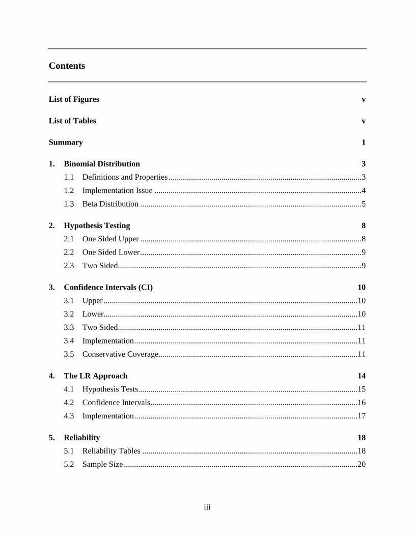
Figure 2 illustrates 𝐶𝐶𝑈𝑈 for 𝑛𝑛 = 10 and 𝛾𝛾 = 0.9.

Figure 2. Upper CI coverage.

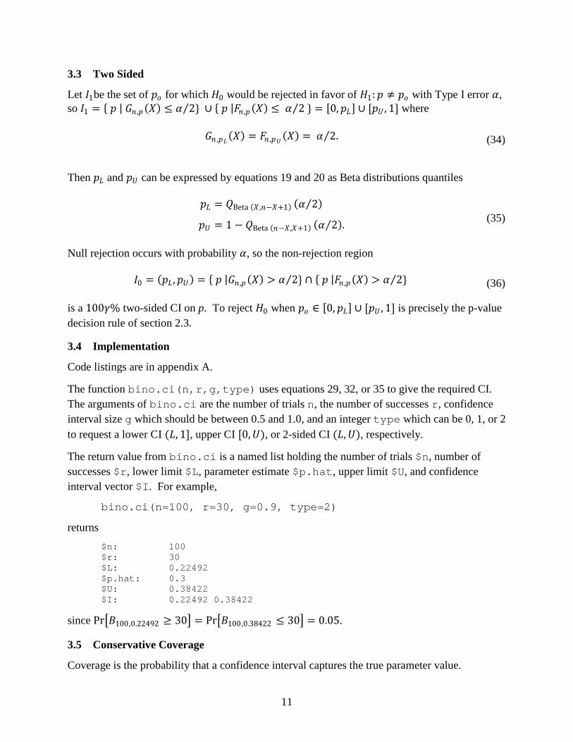
Likewise, 𝑝𝑝𝐿𝐿(𝑋𝑋) is random, and (𝑝𝑝𝐿𝐿(𝑋𝑋), 1] is a 100𝛾𝛾% CI on p. One expects that 𝐶𝐶𝐿𝐿(𝑝𝑝) =Pr[𝑝𝑝𝐿𝐿(𝑋𝑋) < 𝑝𝑝] = E�𝐼𝐼(𝑝𝑝𝐿𝐿(𝑋𝑋),1](𝑝𝑝)� ≥ 𝛾𝛾. This coverage probability is

𝐶𝐶𝐿𝐿(𝑝𝑝) = � Pr[𝑋𝑋 = 𝑘𝑘] ∙ 𝐼𝐼(𝑝𝑝𝐿𝐿(𝑋𝑋),1](𝑝𝑝) = � 𝑓𝑓𝑛𝑛 ,𝑝𝑝(𝑘𝑘)𝑝𝑝𝐿𝐿(𝑘𝑘)<𝑝𝑝

𝑛𝑛

𝑘𝑘=0

. (38)

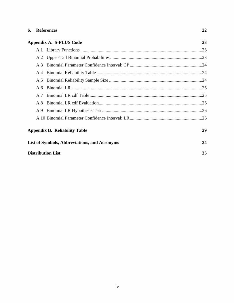
Figure 3 illustrates 𝐶𝐶𝐿𝐿 for 𝑛𝑛 = 10 and 𝛾𝛾 = 0.9.

0.0 0.2 0.4 0.6 0.8 1.0

0.80

0.85

0.90

0.95

1.00

p

C_U(p)

13

Figure 3. Lower CI coverage.

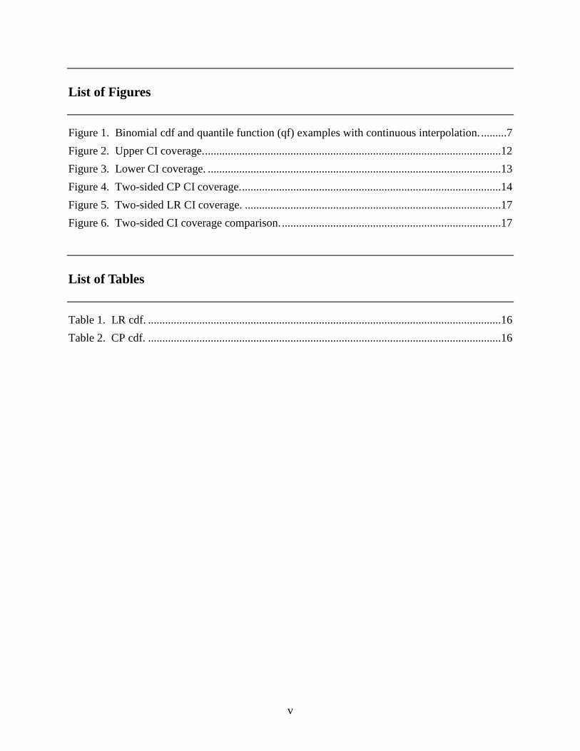
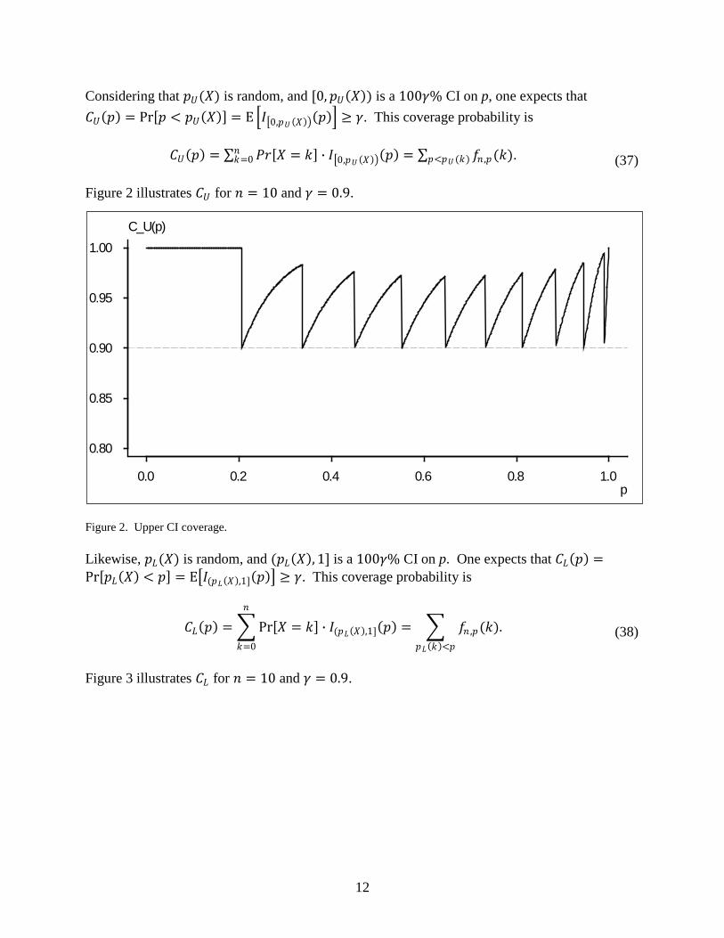
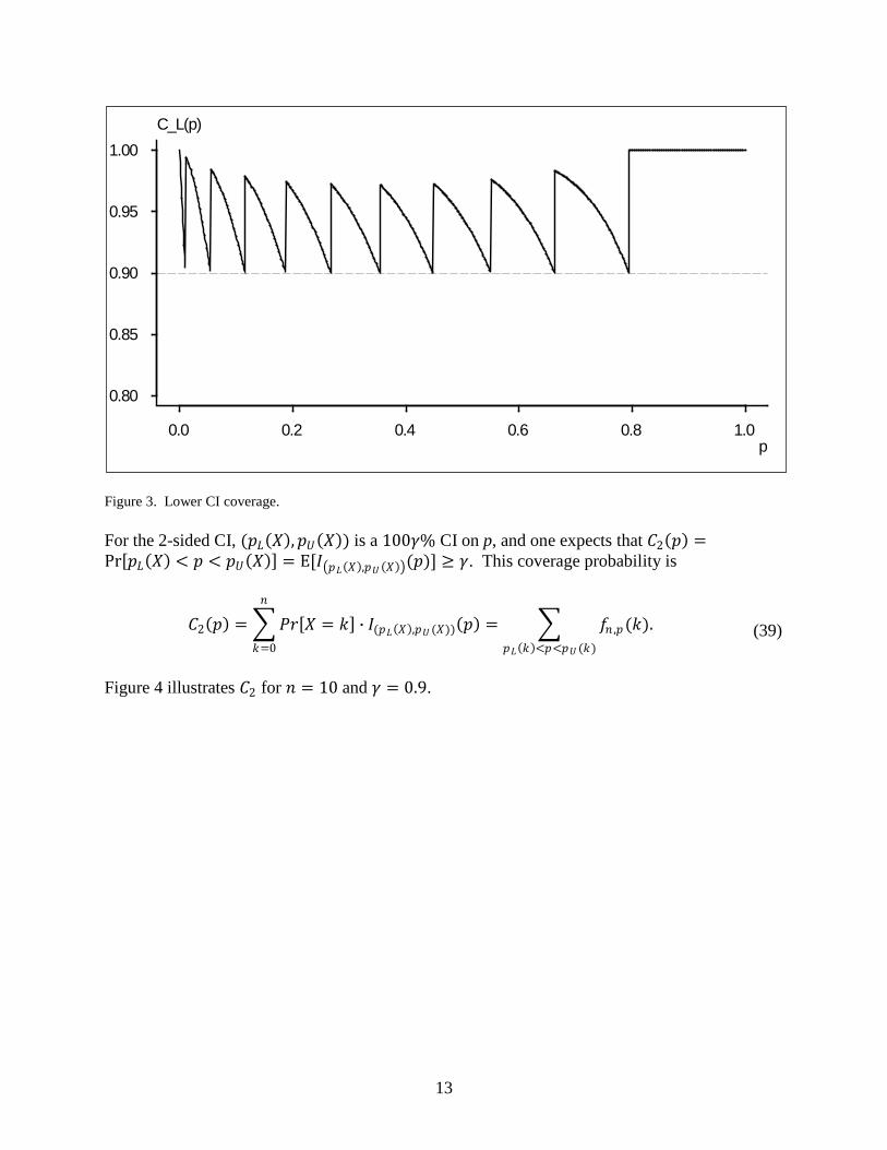
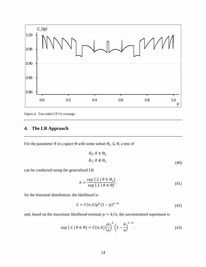
For the 2-sided CI, (𝑝𝑝𝐿𝐿(𝑋𝑋),𝑝𝑝𝑈𝑈(𝑋𝑋)) is a 100𝛾𝛾% CI on p, and one expects that 𝐶𝐶2(𝑝𝑝) =Pr[𝑝𝑝𝐿𝐿(𝑋𝑋) < 𝑝𝑝 < 𝑝𝑝𝑈𝑈(𝑋𝑋)] = E[𝐼𝐼�𝑝𝑝𝐿𝐿(𝑋𝑋),𝑝𝑝𝑈𝑈 (𝑋𝑋)�(𝑝𝑝)] ≥ 𝛾𝛾. This coverage probability is

𝐶𝐶2(𝑝𝑝) = �𝑃𝑃𝑃𝑃[𝑋𝑋 = 𝑘𝑘] ∙ 𝐼𝐼(𝑝𝑝𝐿𝐿(𝑋𝑋),𝑝𝑝𝑈𝑈 (𝑋𝑋))(𝑝𝑝) = � 𝑓𝑓𝑛𝑛 ,𝑝𝑝(𝑘𝑘)𝑝𝑝𝐿𝐿(𝑘𝑘)<𝑝𝑝<𝑝𝑝𝑈𝑈 (𝑘𝑘)

𝑛𝑛

𝑘𝑘=0

. (39)

Figure 4 illustrates 𝐶𝐶2 for 𝑛𝑛 = 10 and 𝛾𝛾 = 0.9.

0.0 0.2 0.4 0.6 0.8 1.0

0.80

0.85

0.90

0.95

1.00

p

C_L(p)

14

Figure 4. Two-sided CP CI coverage.

4. The LR Approach

For the parameter 𝜃𝜃 in a space Θ with some subset Θo ⊆ Θ, a test of

𝐻𝐻0: 𝜃𝜃 ∈ Θ𝑜𝑜

𝐻𝐻1: 𝜃𝜃 ∉ Θ𝑜𝑜 (40)

can be conducted using the generalized LR

Λ =𝑠𝑠𝑢𝑢𝑝𝑝 { ℒ | 𝜃𝜃 ∈ Θ𝑜𝑜}sup { ℒ | 𝜃𝜃 ∈ Θ}

. (41)

for the binomial distribution, the likelihood is

ℒ = 𝐶𝐶(𝑛𝑛, 𝑘𝑘)𝑝𝑝𝑘𝑘(1− 𝑝𝑝)𝑛𝑛−𝑘𝑘 (42)

and, based on the maximum likelihood estimate 𝑝𝑝 = 𝑘𝑘 𝑛𝑛⁄ , the unconstrained supremum is

sup { ℒ | 𝜃𝜃 ∈ Θ} = 𝐶𝐶(𝑛𝑛,𝑘𝑘) �𝑘𝑘𝑛𝑛�𝑘𝑘

�1 −𝑘𝑘𝑛𝑛�𝑛𝑛−𝑘𝑘

. (43)

0.0 0.2 0.4 0.6 0.8 1.0

0.80

0.85

0.90

0.95

1.00

p

C_2(p)

15

For the specific null

𝐻𝐻0 ∶ 𝑝𝑝 = 𝑝𝑝𝑜𝑜 (44)

the conditional supremum is

sup { ℒ | 𝜃𝜃 ∈ 𝛩𝛩𝑜𝑜} = ℒ = 𝐶𝐶(𝑛𝑛,𝑘𝑘) 𝑝𝑝𝑜𝑜 𝑘𝑘(1− 𝑝𝑝𝑜𝑜)𝑛𝑛−𝑘𝑘 . (45)

So the LR is

Λ = �𝑝𝑝𝑜𝑜𝑘𝑘 𝑛𝑛⁄

�𝑘𝑘�

1 − 𝑝𝑝𝑜𝑜1 − 𝑘𝑘 𝑛𝑛⁄

�𝑛𝑛−𝑘𝑘

= �𝑛𝑛𝑝𝑝𝑜𝑜𝑘𝑘�𝑘𝑘�𝑛𝑛 − 𝑛𝑛𝑝𝑝𝑜𝑜𝑛𝑛 − 𝑘𝑘

�𝑛𝑛−𝑘𝑘

. (46)

For data 𝑋𝑋 ∼ 𝐵𝐵𝑛𝑛 ,𝑝𝑝 , the LR is

Λ = �𝑛𝑛𝑝𝑝𝑜𝑜𝑋𝑋�𝑋𝑋�𝑛𝑛 − 𝑛𝑛𝑝𝑝𝑜𝑜𝑛𝑛 − 𝑋𝑋

�𝑛𝑛−𝑋𝑋

. (47)

4.1 Hypothesis Tests

Consider the two-sided test

𝐻𝐻0 ∶ 𝑝𝑝 = 𝑝𝑝𝑜𝑜

𝐻𝐻1 ∶ 𝑝𝑝 ≠ 𝑝𝑝𝑜𝑜 . (48)

Since Λ has small values significant, one rejects 𝐻𝐻0 if Λ ≤ Λ𝑜𝑜 for the appropriate critical value. Note that the null probabilities are Pr[Λ = Λ(𝑘𝑘)] = Pr[𝑋𝑋 = 𝑘𝑘] = 𝑓𝑓𝑛𝑛 ,𝑝𝑝𝑜𝑜 (𝑘𝑘) and the Λ(𝑘𝑘) can be sorted in ascending order and the probabilities summed to obtain the cdf 𝐹𝐹Λ

𝐹𝐹Λ(𝑡𝑡) = � 𝑓𝑓𝑛𝑛 ,𝑝𝑝𝑜𝑜 (𝑘𝑘)Λ(𝑘𝑘)≤𝑡𝑡

= �𝐼𝐼[Λ(𝑘𝑘),1](𝑡𝑡) ∙ 𝑓𝑓𝑛𝑛 ,𝑝𝑝𝑜𝑜 (𝑘𝑘)𝑛𝑛

𝑘𝑘=0

. (49)

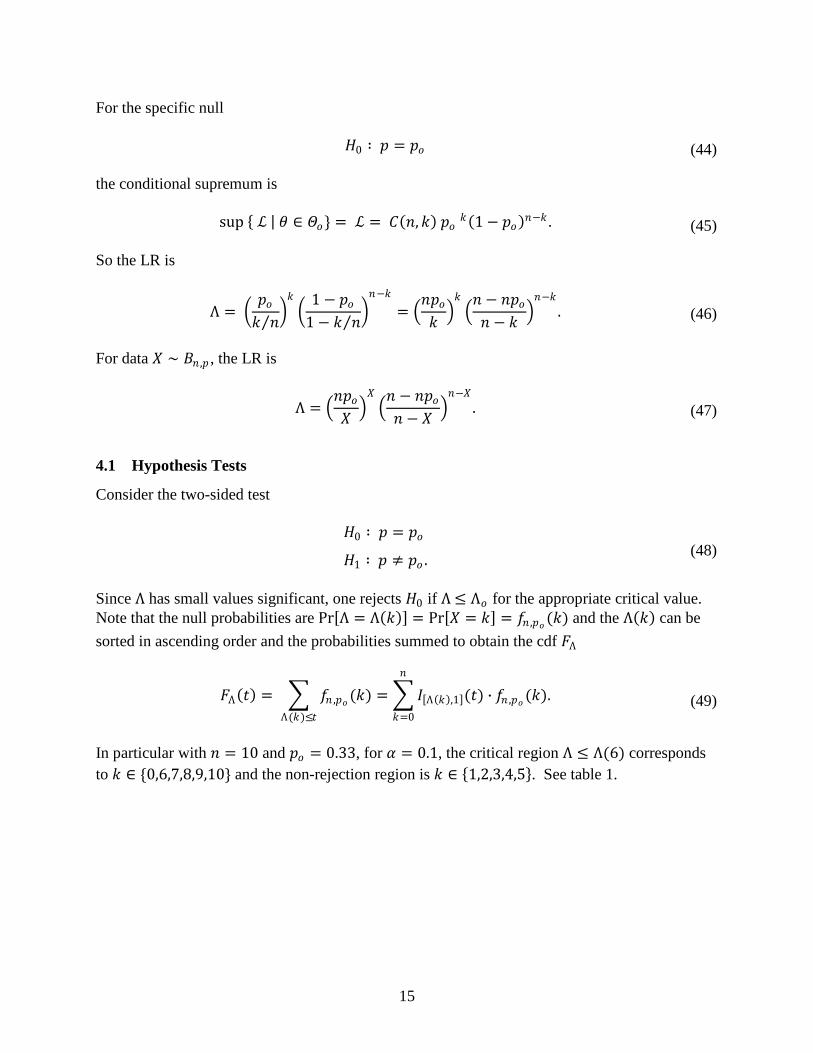
In particular with 𝑛𝑛 = 10 and 𝑝𝑝𝑜𝑜 = 0.33, for 𝛼𝛼 = 0.1, the critical region Λ ≤ Λ(6) corresponds to 𝑘𝑘 ∈ {0,6,7,8,9,10} and the non-rejection region is 𝑘𝑘 ∈ {1,2,3,4,5}. See table 1.

16

Table 1. LR cdf.

𝒌𝒌 𝒇𝒇𝒏𝒏,𝒑𝒑𝒐𝒐(𝒌𝒌) 𝒕𝒕 = 𝚲𝚲(𝒌𝒌) 𝑭𝑭𝚲𝚲(𝒕𝒕) 10 0.01823 0.00002 0.00002 9 0.08978 0.00080 0.00033 8 0.19899 0.00941 0.00317 0 0.26136 0.01823 0.02140 7 0.22528 0.05765 0.03678 6 0.13315 0.21789 0.09143 1 0.05465 0.23174 0.18121 5 0.01538 0.54106 0.31436 2 0.00284 0.65894 0.51335 4 0.00031 0.89817 0.73864 3 0.00002 0.97952 1.00000

Now, based on the usual CP procedure 𝛼𝛼 2⁄ upper and lower tails of the 𝐵𝐵𝑛𝑛 ,𝑝𝑝𝑜𝑜 test statistic, the critical region is {0,7,8,9,10} and the non-rejection region is {1,2,3,4,5,6}. See table 2. Note that 𝑋𝑋 = 6 is critical for the LR test but not for the CP test.

Table 2. CP cdf.

𝒌𝒌 𝑭𝑭𝒏𝒏,𝒑𝒑𝒐𝒐(𝒌𝒌) 𝑮𝑮𝒏𝒏,𝒑𝒑𝒐𝒐(𝒌𝒌) 0 0.01823 1.00000 1 0.10801 0.98177 2 0.30700 0.89199 3 0.56837 0.69300 4 0.79365 0.43163 5 0.92680 0.20635 6 0.98145 0.07320 7 0.99683 0.01855 8 0.99967 0.00317 9 0.99998 0.00033 10 1.00000 0.00002

4.2 Confidence Intervals

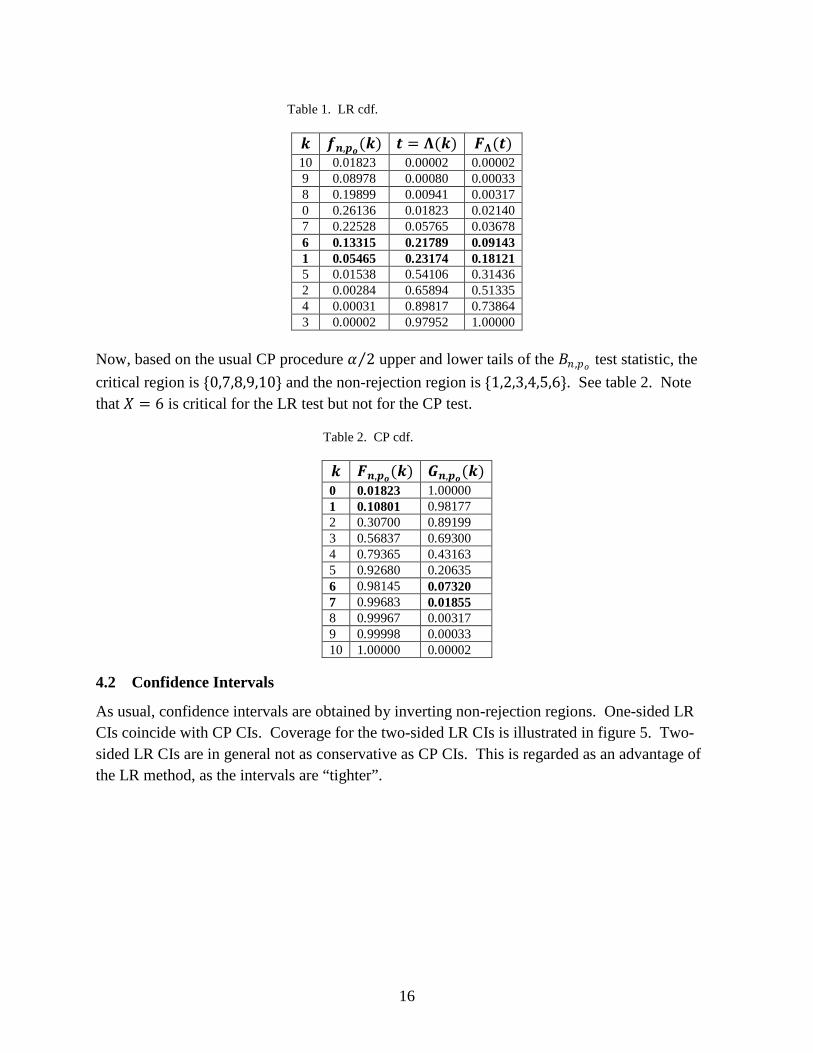
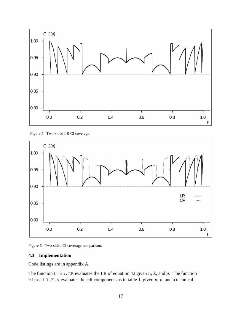
As usual, confidence intervals are obtained by inverting non-rejection regions. One-sided LR CIs coincide with CP CIs. Coverage for the two-sided LR CIs is illustrated in figure 5. Two-sided LR CIs are in general not as conservative as CP CIs. This is regarded as an advantage of the LR method, as the intervals are “tighter”.

17

Figure 5. Two-sided LR CI coverage.

Figure 6. Two-sided CI coverage comparison.

4.3 Implementation

Code listings are in appendix A.

The function bino.LR evaluates the LR of equation 42 given 𝑛𝑛, 𝑘𝑘, and 𝑝𝑝. The function bino.LR.F.x evaluates the cdf components as in table 1, given 𝑛𝑛, 𝑝𝑝, and a technical

0.0 0.2 0.4 0.6 0.8 1.0

0.80

0.85

0.90

0.95

1.00

p

C_2(p)

0.0 0.2 0.4 0.6 0.8 1.0

0.80

0.85

0.90

0.95

1.00

p

C_2(p)

LRCP

18

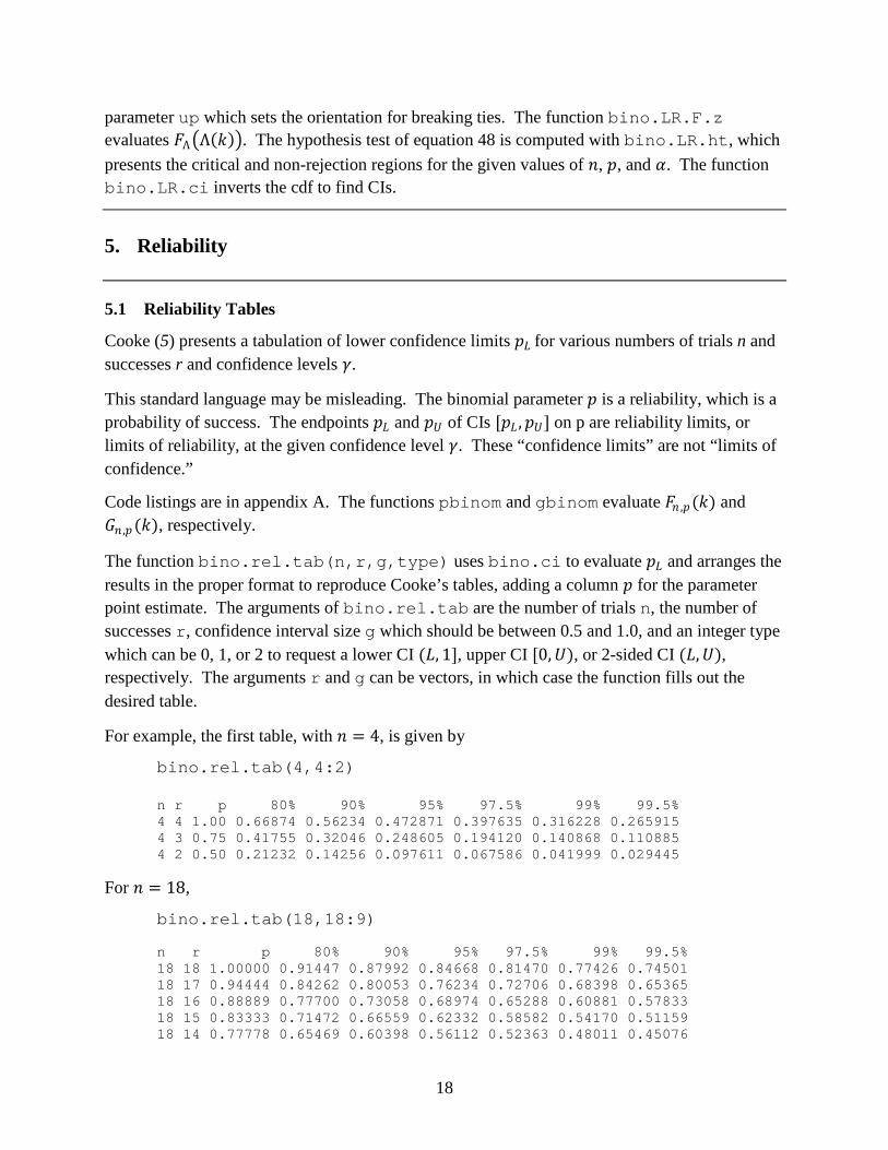
parameter up which sets the orientation for breaking ties. The function bino.LR.F.z evaluates 𝐹𝐹Λ�Λ(𝑘𝑘)�. The hypothesis test of equation 48 is computed with bino.LR.ht, which presents the critical and non-rejection regions for the given values of 𝑛𝑛, 𝑝𝑝, and 𝛼𝛼. The function bino.LR.ci inverts the cdf to find CIs.

5. Reliability

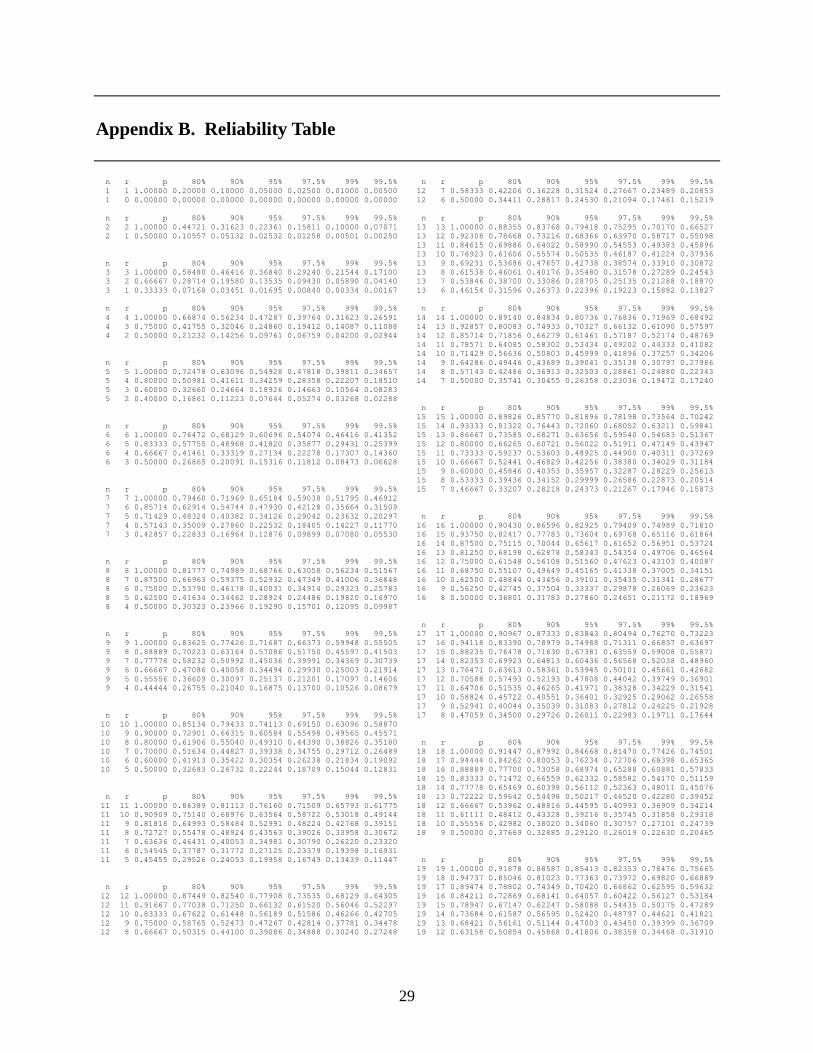
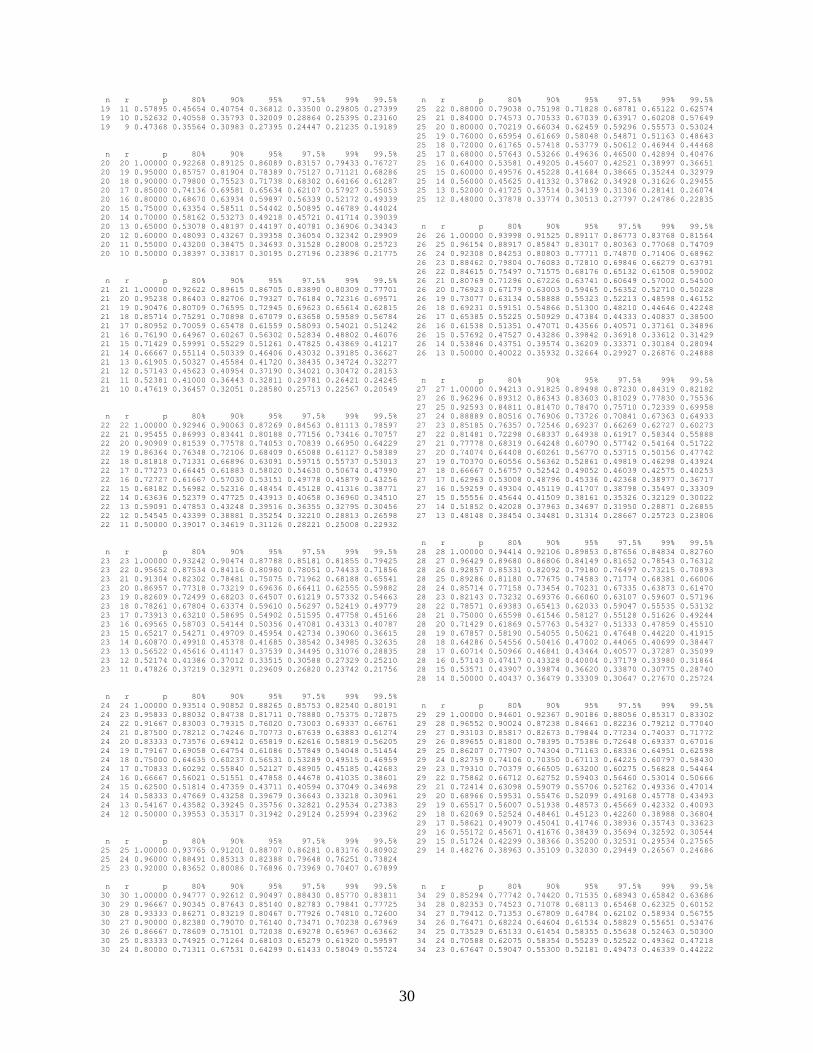
5.1 Reliability Tables

Cooke (5) presents a tabulation of lower confidence limits 𝑝𝑝𝐿𝐿 for various numbers of trials n and successes r and confidence levels 𝛾𝛾.

This standard language may be misleading. The binomial parameter 𝑝𝑝 is a reliability, which is a probability of success. The endpoints 𝑝𝑝𝐿𝐿 and 𝑝𝑝𝑈𝑈 of CIs [𝑝𝑝𝐿𝐿 ,𝑝𝑝𝑈𝑈] on p are reliability limits, or limits of reliability, at the given confidence level 𝛾𝛾. These “confidence limits” are not “limits of confidence.”

Code listings are in appendix A. The functions pbinom and gbinom evaluate 𝐹𝐹𝑛𝑛 ,𝑝𝑝(𝑘𝑘) and 𝐺𝐺𝑛𝑛 ,𝑝𝑝(𝑘𝑘), respectively.

The function bino.rel.tab(n,r,g,type) uses bino.ci to evaluate 𝑝𝑝𝐿𝐿 and arranges the results in the proper format to reproduce Cooke’s tables, adding a column 𝑝𝑝 for the parameter point estimate. The arguments of bino.rel.tab are the number of trials n, the number of successes r, confidence interval size g which should be between 0.5 and 1.0, and an integer type which can be 0, 1, or 2 to request a lower CI (𝐿𝐿, 1], upper CI [0,𝑈𝑈), or 2-sided CI (𝐿𝐿,𝑈𝑈), respectively. The arguments r and g can be vectors, in which case the function fills out the desired table.

For example, the first table, with 𝑛𝑛 = 4, is given by

bino.rel.tab(4,4:2) n r p 80% 90% 95% 97.5% 99% 99.5% 4 4 1.00 0.66874 0.56234 0.472871 0.397635 0.316228 0.265915 4 3 0.75 0.41755 0.32046 0.248605 0.194120 0.140868 0.110885 4 2 0.50 0.21232 0.14256 0.097611 0.067586 0.041999 0.029445

For 𝑛𝑛 = 18,

bino.rel.tab(18,18:9)

n r p 80% 90% 95% 97.5% 99% 99.5% 18 18 1.00000 0.91447 0.87992 0.84668 0.81470 0.77426 0.74501 18 17 0.94444 0.84262 0.80053 0.76234 0.72706 0.68398 0.65365 18 16 0.88889 0.77700 0.73058 0.68974 0.65288 0.60881 0.57833 18 15 0.83333 0.71472 0.66559 0.62332 0.58582 0.54170 0.51159 18 14 0.77778 0.65469 0.60398 0.56112 0.52363 0.48011 0.45076

19

18 13 0.72222 0.59642 0.54498 0.50217 0.46520 0.42280 0.39452 18 12 0.66667 0.53962 0.48816 0.44595 0.40993 0.36909 0.34214 18 11 0.61111 0.48412 0.43328 0.39216 0.35745 0.31858 0.29318 18 10 0.55556 0.42982 0.38020 0.34060 0.30757 0.27101 0.24739 18 9 0.50000 0.37669 0.32885 0.29120 0.26019 0.22630 0.20465

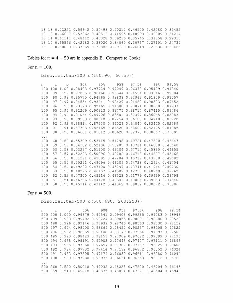
Tables for 𝑛𝑛 = 4 − 50 are in appendix B. Compare to Cooke.

For 𝑛𝑛 = 100,

bino.rel.tab(100,c(100:90, 60:50))

n r p 80% 90% 95% 97.5% 99% 99.5% 100 100 1.00 0.98403 0.97724 0.97049 0.96378 0.95499 0.94840 100 99 0.99 0.97035 0.96166 0.95344 0.94554 0.93546 0.92804 100 98 0.98 0.95770 0.94765 0.93838 0.92962 0.91859 0.91057 100 97 0.97 0.94554 0.93441 0.92429 0.91482 0.90303 0.89452 100 96 0.96 0.93370 0.92165 0.91080 0.90074 0.88830 0.87937 100 95 0.95 0.92209 0.90923 0.89775 0.88717 0.87415 0.86486 100 94 0.94 0.91064 0.89706 0.88501 0.87397 0.86045 0.85083 100 93 0.93 0.89933 0.88510 0.87254 0.86108 0.84710 0.83720 100 92 0.92 0.88814 0.87330 0.86028 0.84844 0.83405 0.82389 100 91 0.91 0.87703 0.86165 0.84820 0.83602 0.82125 0.81085 100 90 0.90 0.86601 0.85012 0.83628 0.82378 0.80867 0.79805 ... 100 60 0.60 0.55309 0.53115 0.51298 0.49721 0.47890 0.46647 100 59 0.59 0.54302 0.52106 0.50289 0.48714 0.46888 0.45648 100 58 0.58 0.53297 0.51100 0.49284 0.47712 0.45890 0.44655 100 57 0.57 0.52293 0.50096 0.48282 0.46713 0.44897 0.43666 100 56 0.56 0.51291 0.49095 0.47284 0.45719 0.43908 0.42682 100 55 0.55 0.50291 0.48096 0.46289 0.44728 0.42924 0.41704 100 54 0.54 0.49292 0.47100 0.45297 0.43741 0.41944 0.40730 100 53 0.53 0.48295 0.46107 0.44309 0.42758 0.40969 0.39762 100 52 0.52 0.47300 0.45116 0.43323 0.41779 0.39999 0.38798 100 51 0.51 0.46306 0.44128 0.42341 0.40804 0.39033 0.37840 100 50 0.50 0.45314 0.43142 0.41362 0.39832 0.38072 0.36886

For 𝑛𝑛 = 500,

bino.rel.tab(500,c(500:490, 260:250))

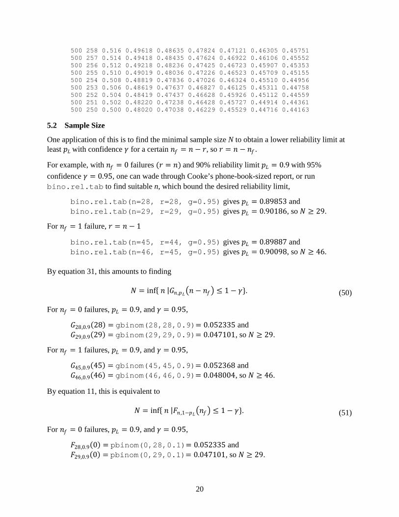
n r p 80% 90% 95% 97.5% 99% 99.5% 500 500 1.000 0.99679 0.99541 0.99403 0.99265 0.99083 0.98946 500 499 0.998 0.99402 0.99224 0.99055 0.98891 0.98680 0.98523 500 498 0.996 0.99146 0.98939 0.98746 0.98563 0.98330 0.98159 500 497 0.994 0.98900 0.98669 0.98457 0.98257 0.98005 0.97822 500 496 0.992 0.98659 0.98408 0.98179 0.97964 0.97697 0.97503 500 495 0.990 0.98423 0.98153 0.97909 0.97682 0.97399 0.97196 500 494 0.988 0.98191 0.97903 0.97645 0.97407 0.97111 0.96898 500 493 0.986 0.97960 0.97657 0.97387 0.97137 0.96829 0.96608 500 492 0.984 0.97732 0.97414 0.97132 0.96872 0.96552 0.96324 500 491 0.982 0.97505 0.97174 0.96880 0.96611 0.96280 0.96044 500 490 0.980 0.97280 0.96935 0.96631 0.96353 0.96012 0.95769 ... 500 260 0.520 0.50018 0.49035 0.48223 0.47520 0.46704 0.46148 500 259 0.518 0.49818 0.48835 0.48024 0.47321 0.46504 0.45949

20

500 258 0.516 0.49618 0.48635 0.47824 0.47121 0.46305 0.45751 500 257 0.514 0.49418 0.48435 0.47624 0.46922 0.46106 0.45552 500 256 0.512 0.49218 0.48236 0.47425 0.46723 0.45907 0.45353 500 255 0.510 0.49019 0.48036 0.47226 0.46523 0.45709 0.45155 500 254 0.508 0.48819 0.47836 0.47026 0.46324 0.45510 0.44956 500 253 0.506 0.48619 0.47637 0.46827 0.46125 0.45311 0.44758 500 252 0.504 0.48419 0.47437 0.46628 0.45926 0.45112 0.44559 500 251 0.502 0.48220 0.47238 0.46428 0.45727 0.44914 0.44361 500 250 0.500 0.48020 0.47038 0.46229 0.45529 0.44716 0.44163

5.2 Sample Size

One application of this is to find the minimal sample size N to obtain a lower reliability limit at least 𝑝𝑝𝐿𝐿 with confidence 𝛾𝛾 for a certain 𝑛𝑛𝑓𝑓 = 𝑛𝑛 − 𝑃𝑃, so 𝑃𝑃 = 𝑛𝑛 − 𝑛𝑛𝑓𝑓 .

For example, with 𝑛𝑛𝑓𝑓 = 0 failures (𝑃𝑃 = 𝑛𝑛) and 90% reliability limit 𝑝𝑝𝐿𝐿 = 0.9 with 95% confidence 𝛾𝛾 = 0.95, one can wade through Cooke’s phone-book-sized report, or run bino.rel.tab to find suitable n, which bound the desired reliability limit,

bino.rel.tab(n=28, r=28, g=0.95) gives 𝑝𝑝𝐿𝐿 = 0.89853 and bino.rel.tab(n=29, r=29, g=0.95) gives 𝑝𝑝𝐿𝐿 = 0.90186, so 𝑁𝑁 ≥ 29.

For 𝑛𝑛𝑓𝑓 = 1 failure, 𝑃𝑃 = 𝑛𝑛 − 1

bino.rel.tab(n=45, r=44, g=0.95) gives 𝑝𝑝𝐿𝐿 = 0.89887 and bino.rel.tab(n=46, r=45, g=0.95) gives 𝑝𝑝𝐿𝐿 = 0.90098, so 𝑁𝑁 ≥ 46.

By equation 31, this amounts to finding

𝑁𝑁 = inf{ 𝑛𝑛 |𝐺𝐺𝑛𝑛 ,𝑝𝑝𝐿𝐿�𝑛𝑛 − 𝑛𝑛𝑓𝑓� ≤ 1 − 𝛾𝛾}. (50)

For 𝑛𝑛𝑓𝑓 = 0 failures, 𝑝𝑝𝐿𝐿 = 0.9, and 𝛾𝛾 = 0.95,

𝐺𝐺28,0.9(28) = gbinom(28,28,0.9)= 0.052335 and 𝐺𝐺29,0.9(29) = gbinom(29,29,0.9)= 0.047101, so 𝑁𝑁 ≥ 29.

For 𝑛𝑛𝑓𝑓 = 1 failures, 𝑝𝑝𝐿𝐿 = 0.9, and 𝛾𝛾 = 0.95,

𝐺𝐺45,0.9(45) = gbinom(45,45,0.9)= 0.052368 and 𝐺𝐺46,0.9(46) = gbinom(46,46,0.9)= 0.048004, so 𝑁𝑁 ≥ 46.

By equation 11, this is equivalent to

𝑁𝑁 = inf{ 𝑛𝑛 |𝐹𝐹𝑛𝑛 ,1−𝑝𝑝𝐿𝐿�𝑛𝑛𝑓𝑓� ≤ 1 − 𝛾𝛾}. (51)

For 𝑛𝑛𝑓𝑓 = 0 failures, 𝑝𝑝𝐿𝐿 = 0.9, and 𝛾𝛾 = 0.95,

𝐹𝐹28,0.9(0) = pbinom(0,28,0.1)= 0.052335 and 𝐹𝐹29,0.9(0) = pbinom(0,29,0.1)= 0.047101, so 𝑁𝑁 ≥ 29.

21

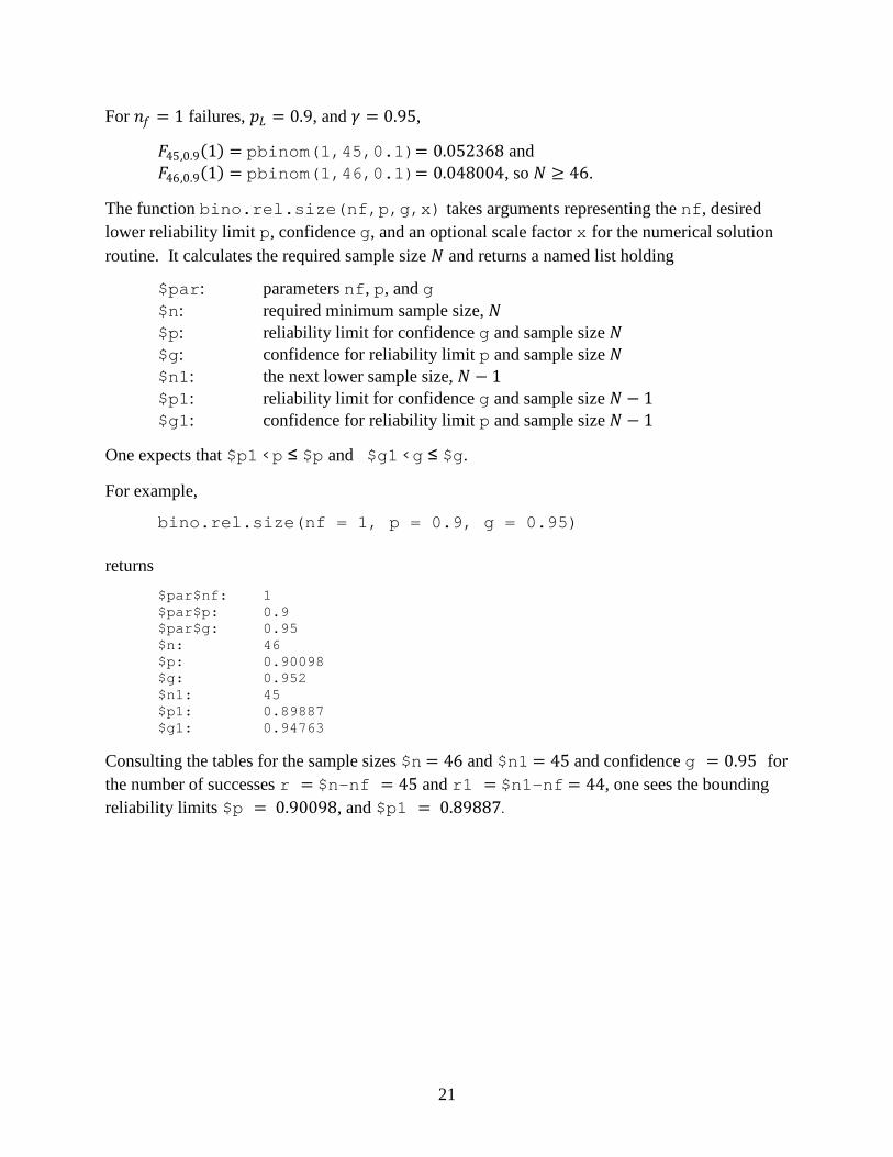
For 𝑛𝑛𝑓𝑓 = 1 failures, 𝑝𝑝𝐿𝐿 = 0.9, and 𝛾𝛾 = 0.95,

𝐹𝐹45,0.9(1) = pbinom(1,45,0.1)= 0.052368 and 𝐹𝐹46,0.9(1) = pbinom(1,46,0.1)= 0.048004, so 𝑁𝑁 ≥ 46.

The function bino.rel.size(nf,p,g,x) takes arguments representing the nf, desired lower reliability limit p, confidence g, and an optional scale factor x for the numerical solution routine. It calculates the required sample size 𝑁𝑁 and returns a named list holding

$par: parameters nf, p, and g $n: required minimum sample size, 𝑁𝑁 $p: reliability limit for confidence g and sample size 𝑁𝑁 $g: confidence for reliability limit p and sample size 𝑁𝑁 $n1: the next lower sample size, 𝑁𝑁 − 1 $p1: reliability limit for confidence g and sample size 𝑁𝑁 − 1 $g1: confidence for reliability limit p and sample size 𝑁𝑁 − 1

One expects that $p1 < p ≤ $p and $g1 < g ≤ $g.

For example,

bino.rel.size(nf = 1, p = 0.9, g = 0.95)

returns $par$nf: 1 $par$p: 0.9 $par$g: 0.95 $n: 46 $p: 0.90098 $g: 0.952 $n1: 45 $p1: 0.89887 $g1: 0.94763

Consulting the tables for the sample sizes $n = 46 and $n1 = 45 and confidence g = 0.95 for the number of successes r = $n-nf = 45 and r1 = $n1-nf = 44, one sees the bounding reliability limits $p = 0.90098, and $p1 = 0.89887.

22

6. References

1. Stuart, A.; Ord, J. K. Kendall’s Advanced Theory of Statistics: Distribution Theory; Oxford University Press: New York, 1994.

2. Mood, A.; Graybill, F. A.; Boes, D. C. Introduction to the Theory of Statistics. 3; McGraw-Hill, New York, 1974.

3. Stuart, A.; Ord, J. K. Kendall’s Advanced Theory of Statistics: Classical Inference and Relationship; Oxford University Press, New York, 1991.

4. Clopper, C. J.; Pearson, E. S. The Use of Confidence or Fiducial Limits Illustrated in the Case of the Binomial. 1934, 4, Biometrika, Vol 26, pp 404–413.

5. Cooke, J. R.; Lee, M. T.; Vanderbeck, J. P. Binomial Reliability Table (Lower Confidence Limits for the Binomial Distribution). China Lake, CA, Bureau of Naval Weapons, 1964.

23

Appendix A. S-PLUS Code

A.1 Library Functions pbinom(q, size = stop("no size arg"), prob = stop("no prob arg"))

is the S-PLUS library implementation of the Binomial distribution cdf.

In the notation of this report,

pbinom(k,n,p)= 𝐹𝐹𝑛𝑛 ,𝑝𝑝(𝑘𝑘) = Pr�𝐵𝐵𝑛𝑛 ,𝑝𝑝 ≤ 𝑘𝑘�

where, k is number of successes, n is the number of trials, and p is the probability of success.

qbeta(p, shape1 = stop("no shape1 arg"), shape2 = stop("no shape2 arg"))

is the S-PLUS library implementation of the Beta distribution qf.

In the notation of this report,

qbeta(u,a,b)= 𝑄𝑄Beta (𝑎𝑎 ,𝑏𝑏)(𝑢𝑢) = inf �𝑥𝑥 ∣ 𝐹𝐹Beta (𝑎𝑎 ,𝑏𝑏)(𝑥𝑥) ≥ 𝑢𝑢 � where, u is the desired probability, and a and b are the usual Beta distribution parameters.

A.2 Upper-Tail Binomial Probabilities

gbinom calculates upper tail binomial probabilities.

gbinom <- function(q,

size = stop("no size arg"), prob = stop("no prob arg")) { ## ## Pr [ Binomial(size,prob) >= q ] ## ## underflow error ## 1-pbinom(q-1,size,prob) ## ## no underflow ## pbinom ( size - q , size , 1 - prob ) }

In the notation of this report,

gbinom(k,n,p)= 𝐺𝐺𝑛𝑛 ,𝑝𝑝(𝑘𝑘) = pbinom(n-k,n,1-p) where, k is number of successes, n is the number of trials, and p is the probability of success.

24

A.3 Binomial Parameter Confidence Interval: CP

bino.ci calculates a CP confidence interval on a binomial parameter estimate.

bino.ci <- function(n , # sample size r , # number of successes g = 0.8 , # CI size type = 0 , # 0,1,2 for lower, upper, 2-sided a = 1-g ) # 1 - (CI size) { ## 100g% Confidence Interval [ L , U ] on Binomial Parameter p ## ## type 0 : lower CI = ( L , 1 ] : Pr [ B(n,L) >= r ] = 1-g ## type 1 : upper CI = [ 0 , U ) : Pr [ B(n,U) <= r ] = 1-g ## type 2 : two-sided CI = (L,U) : Pr[B(n,L)>=r] = Pr[B(n,U)<=r]=(1-g)/2 if(type==2) a <- a/2 if ( type==1 || r==0 ) L <- 0 else L <- qbeta ( a , r , n-r+1 ) if(type==0 || r==n) U <- 1 else U <- 1 - qbeta ( a , n-r , r+1 ) list(n=n, r=r, L=L, p.hat=r/n, U=U, I=c(L,U)) }

A.4 Binomial Reliability Table

bino.rel.tab tabulates binomial confidence limits.

bino.rel.tab <- function(n = 100 , # number of trials r = n , # number of successes g = c(.8,.9,.95,.975,.99,.995),# confidence levels type = 0 ) # 0,1 = lower, upper { nr <- length(r) # success vector length ng <- length(g) # number of CI levels z <- matrix(NA, nc=ng, nr=nr) # reliability limits for( i in 1:nr ) for(j in 1:ng ) # compute reliabilities z[i,j] <- bino.ci(n,r[i],g[j],type)$I[type+1] z <- cbind(n, r, r/n, z) # augmented table dimnames(z) <- # name the table columns list(NULL, c("n","r","p",paste(100*g,"%", sep=""))) z # return table }

A.5 Binomial Reliability Sample Size

bino.rel.size calculates sample size for reliability with a given confidence limit.

25

bino.rel.size <- function(nf = 0 , # number of failures p = 0.9 , # reliability limit g = 0.95 , # confidence level x = 6 ) # log_2 ( search delta ) { ## N = inf { n : pbinom(nf, n, 1-p) } <= 1-g } a <- 1-g # confidence q <- 1-p # reliability f <- function(nf, n, q) list(n=n, a=pbinom(nf, n, q)) # ( n , a ) rtn <- function(nf, p, g, z1, z) # return list list(par=list(nf=nf, p=p, g=g), n=z$n, p=bino.ci(z$n, z$n-nf, g, 0)$L, g=1-z$a , n1=z1$n, p1=bino.ci(z1$n, z1$n-nf, g, 0)$L, g1=1-z1$a) z <- f(nf, 2^x, q) # initial ( n , a ) guess while ( z$a < a ) z <- f(nf, z$n/2, q) while ( z$a > a ) z <- f(nf, z$n*2, q) z0 <- z # upper end at n z1 <- f(nf, z0$n/2, q) # lower end at n/2 dn <- (z0$n-z1$n)/2 # interval radius while ( dn >= 1 ) { z <- f(nf, z1$n+dn, q) # midpoint if ( z$a < a ) # one midpoint becomes new endoint z0 <- z else z1 <- z dn <- dn/2 # new radius } rtn(nf, p, g, z1, z0) }

The algorithm finds sample sizes 𝑛𝑛1 = 2𝑘𝑘−1 and 𝑛𝑛 = 2𝑘𝑘 that bound the confidence for the desired reliability limit. Then it repeatedly bisects the interval [𝑛𝑛1,𝑛𝑛] and replaces one endpoint with the midpoint, maintaining the bound, until 𝑛𝑛 − 𝑛𝑛1 = 1. Reliability limits at the desired confidence level should now bound the desired reliability limit. Using powers of 2 ensures that the sample sizes are integers.

A.6 Binomial LR bino.LR <- function(k , # successes n , # trials p ) # parameter { ## binomial LR ( n*p/k ) ^ k * ( n*(1-p)/(n-k) ) ^ (n-k) }

A.7 Binomial LR cdf Table bino.LR.F.x <- function(n , # trials p , # null parameter up = T ) # tie-breaker direction {

26

## binomial(n,p) LR cdf: complete table k <- 0:n # successes f <- dbinom(k,n,p) # probabilities L <- bino.LR(k,n,p) # LR values if(up) I <- order(L,k) # order LR values, tiebreaker else I <- order(L,-k) L <- L[I] # sort LR values k <- k[I] # order successes by LR value F.L <- cumsum(f[I]) # LR cdf cbind(k, I, f, L, F.L) }

A.8 Binomial LR cdf Evaluation bino.LR.F.z <- function(k , # trials n , # successes p , # null parameter x=F ) # extended return { ## binomial(n,p) LR cdf (k) z <- bino.LR.F.x(n=n, p=p, k>n*p) u <- order(z[,"I"]) if(x) z[u[k+1],] else z[u[k+1],"F.L"] }

A.9 Binomial LR Hypothesis Test bino.LR.ht <- function(n , # trials p , # null parameter a = 0.1 ) # significance { ## binomial LR hypothesis test z <- bino.LR.F.x(n=n, p=p) I.rej <- z[,"F.L"] <= a k.rej <- sort(z[,"k"][I.rej]) k.acc <- sort(z[,"k"][!I.rej]) list(z=z, k.acc=k.acc, k.rej=k.rej) }

A.10 Binomial Parameter Confidence Interval: LR bino.LR.ci <- function(n = 100 , # sample size r = 50 , # number of successes g = 0.9 ) # CI size { h <- r/n q <- 1-g ## [0,h] : L is increasing if(r == 0) p0 <- list(neg=0, pos=0, f0=q, f1=q) else p0 <- uniroot(function(x, n., r., q.) bino.LR.F.z(k=r., n=n., p=x)-q., lower=0, upper=h, q.=q, n.=n, r.=r)

27

## [h,1] : L is decreasing if(r == n) p1 <- list(neg=1, pos=1, f0=q, f1=q) else p1 <- uniroot(function(x, n., r., q.) bino.LR.F.z(k=r., n=n., p=x)-q., lower=h, upper=1, q.=q, n.=n, r.=r) list(n=n, r=r, L=p0$pos, p.hat=h, U=p1$neg, I=c(p0$pos, p1$neg)) }

28

INTENTIONALLY LEFT BLANK.

29

Appendix B. Reliability Table

n r p 80% 90% 95% 97.5% 99% 99.5% n r p 80% 90% 95% 97.5% 99% 99.5% 1 1 1.00000 0.20000 0.10000 0.05000 0.02500 0.01000 0.00500 12 7 0.58333 0.42206 0.36228 0.31524 0.27667 0.23489 0.20853 1 0 0.00000 0.00000 0.00000 0.00000 0.00000 0.00000 0.00000 12 6 0.50000 0.34411 0.28817 0.24530 0.21094 0.17461 0.15219 n r p 80% 90% 95% 97.5% 99% 99.5% n r p 80% 90% 95% 97.5% 99% 99.5% 2 2 1.00000 0.44721 0.31623 0.22361 0.15811 0.10000 0.07071 13 13 1.00000 0.88355 0.83768 0.79418 0.75295 0.70170 0.66527 2 1 0.50000 0.10557 0.05132 0.02532 0.01258 0.00501 0.00250 13 12 0.92308 0.78668 0.73216 0.68366 0.63970 0.58717 0.55098 13 11 0.84615 0.69886 0.64022 0.58990 0.54553 0.49383 0.45896 13 10 0.76923 0.61606 0.55574 0.50535 0.46187 0.41224 0.37936 n r p 80% 90% 95% 97.5% 99% 99.5% 13 9 0.69231 0.53686 0.47657 0.42738 0.38574 0.33910 0.30872 3 3 1.00000 0.58480 0.46416 0.36840 0.29240 0.21544 0.17100 13 8 0.61538 0.46061 0.40176 0.35480 0.31578 0.27289 0.24543 3 2 0.66667 0.28714 0.19580 0.13535 0.09430 0.05890 0.04140 13 7 0.53846 0.38700 0.33086 0.28705 0.25135 0.21288 0.18870 3 1 0.33333 0.07168 0.03451 0.01695 0.00840 0.00334 0.00167 13 6 0.46154 0.31596 0.26373 0.22396 0.19223 0.15882 0.13827 n r p 80% 90% 95% 97.5% 99% 99.5% n r p 80% 90% 95% 97.5% 99% 99.5% 4 4 1.00000 0.66874 0.56234 0.47287 0.39764 0.31623 0.26591 14 14 1.00000 0.89140 0.84834 0.80736 0.76836 0.71969 0.68492 4 3 0.75000 0.41755 0.32046 0.24860 0.19412 0.14087 0.11088 14 13 0.92857 0.80083 0.74933 0.70327 0.66132 0.61090 0.57597 4 2 0.50000 0.21232 0.14256 0.09761 0.06759 0.04200 0.02944 14 12 0.85714 0.71856 0.66279 0.61461 0.57187 0.52174 0.48769 14 11 0.78571 0.64085 0.58302 0.53434 0.49202 0.44333 0.41082 14 10 0.71429 0.56636 0.50803 0.45999 0.41896 0.37257 0.34206 n r p 80% 90% 95% 97.5% 99% 99.5% 14 9 0.64286 0.49446 0.43689 0.39041 0.35138 0.30797 0.27986 5 5 1.00000 0.72478 0.63096 0.54928 0.47818 0.39811 0.34657 14 8 0.57143 0.42486 0.36913 0.32503 0.28861 0.24880 0.22343 5 4 0.80000 0.50981 0.41611 0.34259 0.28358 0.22207 0.18510 14 7 0.50000 0.35741 0.30455 0.26358 0.23036 0.19472 0.17240 5 3 0.60000 0.32660 0.24664 0.18926 0.14663 0.10564 0.08283 5 2 0.40000 0.16861 0.11223 0.07644 0.05274 0.03268 0.02288 n r p 80% 90% 95% 97.5% 99% 99.5% 15 15 1.00000 0.89826 0.85770 0.81896 0.78198 0.73564 0.70242 n r p 80% 90% 95% 97.5% 99% 99.5% 15 14 0.93333 0.81322 0.76443 0.72060 0.68052 0.63211 0.59841 6 6 1.00000 0.76472 0.68129 0.60696 0.54074 0.46416 0.41352 15 13 0.86667 0.73585 0.68271 0.63656 0.59540 0.54683 0.51367 6 5 0.83333 0.57755 0.48968 0.41820 0.35877 0.29431 0.25399 15 12 0.80000 0.66265 0.60721 0.56022 0.51911 0.47149 0.43947 6 4 0.66667 0.41461 0.33319 0.27134 0.22278 0.17307 0.14360 15 11 0.73333 0.59237 0.53603 0.48925 0.44900 0.40311 0.37269 6 3 0.50000 0.26865 0.20091 0.15316 0.11812 0.08473 0.06628 15 10 0.66667 0.52441 0.46829 0.42256 0.38380 0.34029 0.31184 15 9 0.60000 0.45846 0.40353 0.35957 0.32287 0.28229 0.25613 15 8 0.53333 0.39436 0.34152 0.29999 0.26586 0.22873 0.20514 n r p 80% 90% 95% 97.5% 99% 99.5% 15 7 0.46667 0.33207 0.28218 0.24373 0.21267 0.17946 0.15873 7 7 1.00000 0.79460 0.71969 0.65184 0.59038 0.51795 0.46912 7 6 0.85714 0.62914 0.54744 0.47930 0.42128 0.35664 0.31509 7 5 0.71429 0.48324 0.40382 0.34126 0.29042 0.23632 0.20297 n r p 80% 90% 95% 97.5% 99% 99.5% 7 4 0.57143 0.35009 0.27860 0.22532 0.18405 0.14227 0.11770 16 16 1.00000 0.90430 0.86596 0.82925 0.79409 0.74989 0.71810 7 3 0.42857 0.22833 0.16964 0.12876 0.09899 0.07080 0.05530 16 15 0.93750 0.82417 0.77783 0.73604 0.69768 0.65116 0.61864 16 14 0.87500 0.75115 0.70044 0.65617 0.61652 0.56951 0.53724 16 13 0.81250 0.68198 0.62878 0.58343 0.54354 0.49706 0.46564 n r p 80% 90% 95% 97.5% 99% 99.5% 16 12 0.75000 0.61548 0.56108 0.51560 0.47623 0.43103 0.40087 8 8 1.00000 0.81777 0.74989 0.68766 0.63058 0.56234 0.51567 16 11 0.68750 0.55107 0.49649 0.45165 0.41338 0.37005 0.34151 8 7 0.87500 0.66963 0.59375 0.52932 0.47349 0.41006 0.36848 16 10 0.62500 0.48844 0.43456 0.39101 0.35435 0.31341 0.28677 8 6 0.75000 0.53790 0.46178 0.40031 0.34914 0.29323 0.25783 16 9 0.56250 0.42745 0.37504 0.33337 0.29878 0.26069 0.23623 8 5 0.62500 0.41634 0.34462 0.28924 0.24486 0.19820 0.16970 16 8 0.50000 0.36801 0.31783 0.27860 0.24651 0.21172 0.18969 8 4 0.50000 0.30323 0.23966 0.19290 0.15701 0.12095 0.09987 n r p 80% 90% 95% 97.5% 99% 99.5% n r p 80% 90% 95% 97.5% 99% 99.5% 17 17 1.00000 0.90967 0.87333 0.83843 0.80494 0.76270 0.73223 9 9 1.00000 0.83625 0.77426 0.71687 0.66373 0.59948 0.55505 17 16 0.94118 0.83390 0.78979 0.74988 0.71311 0.66837 0.63697 9 8 0.88889 0.70223 0.63164 0.57086 0.51750 0.45597 0.41503 17 15 0.88235 0.76478 0.71630 0.67381 0.63559 0.59008 0.55871 9 7 0.77778 0.58232 0.50992 0.45036 0.39991 0.34369 0.30739 17 14 0.82353 0.69923 0.64813 0.60436 0.56568 0.52038 0.48960 9 6 0.66667 0.47086 0.40058 0.34494 0.29930 0.25003 0.21914 17 13 0.76471 0.63613 0.58361 0.53945 0.50101 0.45661 0.42682 9 5 0.55556 0.36609 0.30097 0.25137 0.21201 0.17097 0.14606 17 12 0.70588 0.57493 0.52193 0.47808 0.44042 0.39749 0.36901 9 4 0.44444 0.26755 0.21040 0.16875 0.13700 0.10526 0.08679 17 11 0.64706 0.51535 0.46265 0.41971 0.38328 0.34229 0.31541 17 10 0.58824 0.45722 0.40551 0.36401 0.32925 0.29062 0.26558 17 9 0.52941 0.40044 0.35039 0.31083 0.27812 0.24225 0.21928 n r p 80% 90% 95% 97.5% 99% 99.5% 17 8 0.47059 0.34500 0.29726 0.26011 0.22983 0.19711 0.17644 10 10 1.00000 0.85134 0.79433 0.74113 0.69150 0.63096 0.58870 10 9 0.90000 0.72901 0.66315 0.60584 0.55498 0.49565 0.45571 10 8 0.80000 0.61906 0.55040 0.49310 0.44390 0.38826 0.35180 n r p 80% 90% 95% 97.5% 99% 99.5% 10 7 0.70000 0.51634 0.44827 0.39338 0.34755 0.29712 0.26489 18 18 1.00000 0.91447 0.87992 0.84668 0.81470 0.77426 0.74501 10 6 0.60000 0.41913 0.35422 0.30354 0.26238 0.21834 0.19092 18 17 0.94444 0.84262 0.80053 0.76234 0.72706 0.68398 0.65365 10 5 0.50000 0.32683 0.26732 0.22244 0.18709 0.15044 0.12831 18 16 0.88889 0.77700 0.73058 0.68974 0.65288 0.60881 0.57833 18 15 0.83333 0.71472 0.66559 0.62332 0.58582 0.54170 0.51159 18 14 0.77778 0.65469 0.60398 0.56112 0.52363 0.48011 0.45076 n r p 80% 90% 95% 97.5% 99% 99.5% 18 13 0.72222 0.59642 0.54498 0.50217 0.46520 0.42280 0.39452 11 11 1.00000 0.86389 0.81113 0.76160 0.71509 0.65793 0.61775 18 12 0.66667 0.53962 0.48816 0.44595 0.40993 0.36909 0.34214 11 10 0.90909 0.75140 0.68976 0.63564 0.58722 0.53018 0.49144 18 11 0.61111 0.48412 0.43328 0.39216 0.35745 0.31858 0.29318 11 9 0.81818 0.64993 0.58484 0.52991 0.48224 0.42768 0.39151 18 10 0.55556 0.42982 0.38020 0.34060 0.30757 0.27101 0.24739 11 8 0.72727 0.55478 0.48924 0.43563 0.39026 0.33958 0.30672 18 9 0.50000 0.37669 0.32885 0.29120 0.26019 0.22630 0.20465 11 7 0.63636 0.46431 0.40053 0.34981 0.30790 0.26220 0.23320 11 6 0.54545 0.37787 0.31772 0.27125 0.23379 0.19398 0.16931 11 5 0.45455 0.29526 0.24053 0.19958 0.16749 0.13439 0.11447 n r p 80% 90% 95% 97.5% 99% 99.5% 19 19 1.00000 0.91878 0.88587 0.85413 0.82353 0.78476 0.75665 19 18 0.94737 0.85046 0.81023 0.77363 0.73972 0.69820 0.66889 n r p 80% 90% 95% 97.5% 99% 99.5% 19 17 0.89474 0.78802 0.74349 0.70420 0.66862 0.62595 0.59632 12 12 1.00000 0.87449 0.82540 0.77908 0.73535 0.68129 0.64305 19 16 0.84211 0.72869 0.68141 0.64057 0.60422 0.56127 0.53184 12 11 0.91667 0.77038 0.71250 0.66132 0.61520 0.56046 0.52297 19 15 0.78947 0.67147 0.62247 0.58088 0.54435 0.50175 0.47289 12 10 0.83333 0.67622 0.61448 0.56189 0.51586 0.46266 0.42705 19 14 0.73684 0.61587 0.56595 0.52420 0.48797 0.44621 0.41821 12 9 0.75000 0.58765 0.52473 0.47267 0.42814 0.37781 0.34478 19 13 0.68421 0.56161 0.51144 0.47003 0.43450 0.39399 0.36709 12 8 0.66667 0.50315 0.44100 0.39086 0.34888 0.30240 0.27248 19 12 0.63158 0.50854 0.45868 0.41806 0.38358 0.34468 0.31910

30

n r p 80% 90% 95% 97.5% 99% 99.5% n r p 80% 90% 95% 97.5% 99% 99.5% 19 11 0.57895 0.45654 0.40754 0.36812 0.33500 0.29805 0.27399 25 22 0.88000 0.79038 0.75198 0.71828 0.68781 0.65122 0.62574 19 10 0.52632 0.40558 0.35793 0.32009 0.28864 0.25395 0.23160 25 21 0.84000 0.74573 0.70533 0.67039 0.63917 0.60208 0.57649 19 9 0.47368 0.35564 0.30983 0.27395 0.24447 0.21235 0.19189 25 20 0.80000 0.70219 0.66034 0.62459 0.59296 0.55573 0.53024 25 19 0.76000 0.65954 0.61669 0.58048 0.54871 0.51163 0.48643 25 18 0.72000 0.61765 0.57418 0.53779 0.50612 0.46944 0.44468 n r p 80% 90% 95% 97.5% 99% 99.5% 25 17 0.68000 0.57643 0.53266 0.49636 0.46500 0.42894 0.40476 20 20 1.00000 0.92268 0.89125 0.86089 0.83157 0.79433 0.76727 25 16 0.64000 0.53581 0.49205 0.45607 0.42521 0.38997 0.36651 20 19 0.95000 0.85757 0.81904 0.78389 0.75127 0.71121 0.68286 25 15 0.60000 0.49576 0.45228 0.41684 0.38665 0.35244 0.32979 20 18 0.90000 0.79800 0.75523 0.71738 0.68302 0.64166 0.61287 25 14 0.56000 0.45625 0.41332 0.37862 0.34928 0.31626 0.29455 20 17 0.85000 0.74136 0.69581 0.65634 0.62107 0.57927 0.55053 25 13 0.52000 0.41725 0.37514 0.34139 0.31306 0.28141 0.26074 20 16 0.80000 0.68670 0.63934 0.59897 0.56339 0.52172 0.49339 25 12 0.48000 0.37878 0.33774 0.30513 0.27797 0.24786 0.22835 20 15 0.75000 0.63354 0.58511 0.54442 0.50895 0.46789 0.44024 20 14 0.70000 0.58162 0.53273 0.49218 0.45721 0.41714 0.39039 20 13 0.65000 0.53078 0.48197 0.44197 0.40781 0.36906 0.34343 n r p 80% 90% 95% 97.5% 99% 99.5% 20 12 0.60000 0.48093 0.43267 0.39358 0.36054 0.32342 0.29909 26 26 1.00000 0.93998 0.91525 0.89117 0.86773 0.83768 0.81564 20 11 0.55000 0.43200 0.38475 0.34693 0.31528 0.28008 0.25723 26 25 0.96154 0.88917 0.85847 0.83017 0.80363 0.77068 0.74709 20 10 0.50000 0.38397 0.33817 0.30195 0.27196 0.23896 0.21775 26 24 0.92308 0.84253 0.80803 0.77711 0.74870 0.71406 0.68962 26 23 0.88462 0.79804 0.76083 0.72810 0.69846 0.66279 0.63791 26 22 0.84615 0.75497 0.71575 0.68176 0.65132 0.61508 0.59002 n r p 80% 90% 95% 97.5% 99% 99.5% 26 21 0.80769 0.71296 0.67226 0.63741 0.60649 0.57002 0.54500 21 21 1.00000 0.92622 0.89615 0.86705 0.83890 0.80309 0.77701 26 20 0.76923 0.67179 0.63003 0.59465 0.56352 0.52710 0.50228 21 20 0.95238 0.86403 0.82706 0.79327 0.76184 0.72316 0.69571 26 19 0.73077 0.63134 0.58888 0.55323 0.52213 0.48598 0.46152 21 19 0.90476 0.80709 0.76595 0.72945 0.69623 0.65614 0.62815 26 18 0.69231 0.59151 0.54866 0.51300 0.48210 0.44646 0.42248 21 18 0.85714 0.75291 0.70898 0.67079 0.63658 0.59589 0.56784 26 17 0.65385 0.55225 0.50929 0.47384 0.44333 0.40837 0.38500 21 17 0.80952 0.70059 0.65478 0.61559 0.58093 0.54021 0.51242 26 16 0.61538 0.51351 0.47071 0.43566 0.40571 0.37161 0.34896 21 16 0.76190 0.64967 0.60267 0.56302 0.52834 0.48802 0.46076 26 15 0.57692 0.47527 0.43286 0.39842 0.36918 0.33612 0.31429 21 15 0.71429 0.59991 0.55229 0.51261 0.47825 0.43869 0.41217 26 14 0.53846 0.43751 0.39574 0.36209 0.33371 0.30184 0.28094 21 14 0.66667 0.55114 0.50339 0.46406 0.43032 0.39185 0.36627 26 13 0.50000 0.40022 0.35932 0.32664 0.29927 0.26876 0.24888 21 13 0.61905 0.50327 0.45584 0.41720 0.38435 0.34724 0.32277 21 12 0.57143 0.45623 0.40954 0.37190 0.34021 0.30472 0.28153 21 11 0.52381 0.41000 0.36443 0.32811 0.29781 0.26421 0.24245 n r p 80% 90% 95% 97.5% 99% 99.5% 21 10 0.47619 0.36457 0.32051 0.28580 0.25713 0.22567 0.20549 27 27 1.00000 0.94213 0.91825 0.89498 0.87230 0.84319 0.82182 27 26 0.96296 0.89312 0.86343 0.83603 0.81029 0.77830 0.75536 27 25 0.92593 0.84811 0.81470 0.78470 0.75710 0.72339 0.69958 n r p 80% 90% 95% 97.5% 99% 99.5% 27 24 0.88889 0.80516 0.76906 0.73726 0.70841 0.67363 0.64933 22 22 1.00000 0.92946 0.90063 0.87269 0.84563 0.81113 0.78597 27 23 0.85185 0.76357 0.72546 0.69237 0.66269 0.62727 0.60273 22 21 0.95455 0.86993 0.83441 0.80188 0.77156 0.73416 0.70757 27 22 0.81481 0.72298 0.68337 0.64938 0.61917 0.58344 0.55888 22 20 0.90909 0.81539 0.77578 0.74053 0.70839 0.66950 0.64229 27 21 0.77778 0.68319 0.64248 0.60790 0.57742 0.54164 0.51722 22 19 0.86364 0.76348 0.72106 0.68409 0.65088 0.61127 0.58389 27 20 0.74074 0.64408 0.60261 0.56770 0.53715 0.50156 0.47742 22 18 0.81818 0.71331 0.66896 0.63091 0.59715 0.55737 0.53013 27 19 0.70370 0.60556 0.56362 0.52861 0.49819 0.46298 0.43924 22 17 0.77273 0.66445 0.61883 0.58020 0.54630 0.50674 0.47990 27 18 0.66667 0.56757 0.52542 0.49052 0.46039 0.42575 0.40253 22 16 0.72727 0.61667 0.57030 0.53151 0.49778 0.45879 0.43256 27 17 0.62963 0.53008 0.48796 0.45336 0.42368 0.38977 0.36717 22 15 0.68182 0.56982 0.52316 0.48454 0.45128 0.41316 0.38771 27 16 0.59259 0.49304 0.45119 0.41707 0.38798 0.35497 0.33309 22 14 0.63636 0.52379 0.47725 0.43913 0.40658 0.36960 0.34510 27 15 0.55556 0.45644 0.41509 0.38161 0.35326 0.32129 0.30022 22 13 0.59091 0.47853 0.43248 0.39516 0.36355 0.32795 0.30456 27 14 0.51852 0.42028 0.37963 0.34697 0.31950 0.28871 0.26855 22 12 0.54545 0.43399 0.38881 0.35254 0.32210 0.28813 0.26598 27 13 0.48148 0.38454 0.34481 0.31314 0.28667 0.25723 0.23806 22 11 0.50000 0.39017 0.34619 0.31126 0.28221 0.25008 0.22932 n r p 80% 90% 95% 97.5% 99% 99.5% n r p 80% 90% 95% 97.5% 99% 99.5% 28 28 1.00000 0.94414 0.92106 0.89853 0.87656 0.84834 0.82760 23 23 1.00000 0.93242 0.90474 0.87788 0.85181 0.81855 0.79425 28 27 0.96429 0.89680 0.86806 0.84149 0.81652 0.78543 0.76312 23 22 0.95652 0.87534 0.84116 0.80980 0.78051 0.74433 0.71856 28 26 0.92857 0.85331 0.82092 0.79180 0.76497 0.73215 0.70893 23 21 0.91304 0.82302 0.78481 0.75075 0.71962 0.68188 0.65541 28 25 0.89286 0.81180 0.77675 0.74583 0.71774 0.68381 0.66006 23 20 0.86957 0.77318 0.73219 0.69636 0.66411 0.62555 0.59882 28 24 0.85714 0.77158 0.73454 0.70231 0.67335 0.63873 0.61470 23 19 0.82609 0.72499 0.68203 0.64507 0.61219 0.57332 0.54663 28 23 0.82143 0.73232 0.69376 0.66060 0.63107 0.59607 0.57196 23 18 0.78261 0.67804 0.63374 0.59610 0.56297 0.52419 0.49779 28 22 0.78571 0.69383 0.65413 0.62033 0.59047 0.55535 0.53132 23 17 0.73913 0.63210 0.58695 0.54902 0.51595 0.47758 0.45166 28 21 0.75000 0.65598 0.61546 0.58127 0.55128 0.51626 0.49244 23 16 0.69565 0.58703 0.54144 0.50356 0.47081 0.43313 0.40787 28 20 0.71429 0.61869 0.57763 0.54327 0.51333 0.47859 0.45510 23 15 0.65217 0.54271 0.49709 0.45954 0.42734 0.39060 0.36615 28 19 0.67857 0.58190 0.54055 0.50621 0.47648 0.44220 0.41915 23 14 0.60870 0.49910 0.45378 0.41685 0.38542 0.34985 0.32635 28 18 0.64286 0.54556 0.50416 0.47002 0.44065 0.40699 0.38447 23 13 0.56522 0.45616 0.41147 0.37539 0.34495 0.31076 0.28835 28 17 0.60714 0.50966 0.46841 0.43464 0.40577 0.37287 0.35099 23 12 0.52174 0.41386 0.37012 0.33515 0.30588 0.27329 0.25210 28 16 0.57143 0.47417 0.43328 0.40004 0.37179 0.33980 0.31864 23 11 0.47826 0.37219 0.32971 0.29609 0.26820 0.23742 0.21756 28 15 0.53571 0.43907 0.39874 0.36620 0.33870 0.30775 0.28740 28 14 0.50000 0.40437 0.36479 0.33309 0.30647 0.27670 0.25724 n r p 80% 90% 95% 97.5% 99% 99.5% 24 24 1.00000 0.93514 0.90852 0.88265 0.85753 0.82540 0.80191 n r p 80% 90% 95% 97.5% 99% 99.5% 24 23 0.95833 0.88032 0.84738 0.81711 0.78880 0.75375 0.72875 29 29 1.00000 0.94601 0.92367 0.90186 0.88056 0.85317 0.83302 24 22 0.91667 0.83003 0.79315 0.76020 0.73003 0.69337 0.66761 29 28 0.96552 0.90024 0.87238 0.84661 0.82236 0.79212 0.77040 24 21 0.87500 0.78212 0.74246 0.70773 0.67639 0.63883 0.61274 29 27 0.93103 0.85817 0.82673 0.79844 0.77234 0.74037 0.71772 24 20 0.83333 0.73576 0.69412 0.65819 0.62616 0.58819 0.56205 29 26 0.89655 0.81800 0.78395 0.75386 0.72648 0.69337 0.67016 24 19 0.79167 0.69058 0.64754 0.61086 0.57849 0.54048 0.51454 29 25 0.86207 0.77907 0.74304 0.71163 0.68336 0.64951 0.62598 24 18 0.75000 0.64635 0.60237 0.56531 0.53289 0.49515 0.46959 29 24 0.82759 0.74106 0.70350 0.67113 0.64225 0.60797 0.58430 24 17 0.70833 0.60292 0.55840 0.52127 0.48905 0.45185 0.42683 29 23 0.79310 0.70379 0.66505 0.63200 0.60275 0.56828 0.54464 24 16 0.66667 0.56021 0.51551 0.47858 0.44678 0.41035 0.38601 29 22 0.75862 0.66712 0.62752 0.59403 0.56460 0.53014 0.50666 24 15 0.62500 0.51814 0.47359 0.43711 0.40594 0.37049 0.34698 29 21 0.72414 0.63098 0.59079 0.55706 0.52762 0.49336 0.47014 24 14 0.58333 0.47669 0.43258 0.39679 0.36643 0.33218 0.30961 29 20 0.68966 0.59531 0.55476 0.52099 0.49168 0.45778 0.43493 24 13 0.54167 0.43582 0.39245 0.35756 0.32821 0.29534 0.27383 29 19 0.65517 0.56007 0.51938 0.48573 0.45669 0.42332 0.40093 24 12 0.50000 0.39553 0.35317 0.31942 0.29124 0.25994 0.23962 29 18 0.62069 0.52524 0.48461 0.45123 0.42260 0.38988 0.36804 29 17 0.58621 0.49079 0.45041 0.41746 0.38936 0.35743 0.33623 29 16 0.55172 0.45671 0.41676 0.38439 0.35694 0.32592 0.30544 n r p 80% 90% 95% 97.5% 99% 99.5% 29 15 0.51724 0.42299 0.38366 0.35200 0.32531 0.29534 0.27565 25 25 1.00000 0.93765 0.91201 0.88707 0.86281 0.83176 0.80902 29 14 0.48276 0.38963 0.35109 0.32030 0.29449 0.26567 0.24686 25 24 0.96000 0.88491 0.85313 0.82388 0.79648 0.76251 0.73824 25 23 0.92000 0.83652 0.80086 0.76896 0.73969 0.70407 0.67899 n r p 80% 90% 95% 97.5% 99% 99.5% n r p 80% 90% 95% 97.5% 99% 99.5% 30 30 1.00000 0.94777 0.92612 0.90497 0.88430 0.85770 0.83811 34 29 0.85294 0.77742 0.74420 0.71535 0.68943 0.65842 0.63686 30 29 0.96667 0.90345 0.87643 0.85140 0.82783 0.79841 0.77725 34 28 0.82353 0.74523 0.71078 0.68113 0.65468 0.62325 0.60152 30 28 0.93333 0.86271 0.83219 0.80467 0.77926 0.74810 0.72600 34 27 0.79412 0.71353 0.67809 0.64784 0.62102 0.58934 0.56755 30 27 0.90000 0.82380 0.79070 0.76140 0.73471 0.70238 0.67969 34 26 0.76471 0.68224 0.64604 0.61534 0.58829 0.55651 0.53476 30 26 0.86667 0.78609 0.75101 0.72038 0.69278 0.65967 0.63662 34 25 0.73529 0.65133 0.61454 0.58355 0.55638 0.52463 0.50300 30 25 0.83333 0.74925 0.71264 0.68103 0.65279 0.61920 0.59597 34 24 0.70588 0.62075 0.58354 0.55239 0.52522 0.49362 0.47218 30 24 0.80000 0.71311 0.67531 0.64299 0.61433 0.58049 0.55724 34 23 0.67647 0.59047 0.55300 0.52181 0.49473 0.46339 0.44222

31

30 23 0.76667 0.67756 0.63886 0.60605 0.57716 0.54327 0.52012 34 22 0.64706 0.56048 0.52289 0.49177 0.46489 0.43390 0.41306 30 22 0.73333 0.64250 0.60316 0.57007 0.54111 0.50734 0.48440 34 21 0.61765 0.53076 0.49318 0.46225 0.43564 0.40512 0.38467 30 21 0.70000 0.60790 0.56813 0.53493 0.50604 0.47256 0.44992 34 20 0.58824 0.50130 0.46386 0.43321 0.40697 0.37700 0.35700 30 20 0.66667 0.57370 0.53372 0.50056 0.47188 0.43882 0.41658 34 19 0.55882 0.47209 0.43492 0.40466 0.37886 0.34953 0.33004 30 19 0.63333 0.53988 0.49987 0.46691 0.43856 0.40605 0.38430 34 18 0.52941 0.44312 0.40635 0.37657 0.35129 0.32269 0.30377 30 18 0.60000 0.50642 0.46657 0.43395 0.40603 0.37421 0.35302 34 17 0.50000 0.41440 0.37814 0.34894 0.32427 0.29649 0.27819 30 17 0.56667 0.47330 0.43378 0.40163 0.37427 0.34325 0.32270 30 16 0.53333 0.44052 0.40149 0.36995 0.34326 0.31315 0.29331 30 15 0.50000 0.40807 0.36970 0.33889 0.31297 0.28390 0.26485 n r p 80% 90% 95% 97.5% 99% 99.5% 35 35 1.00000 0.95506 0.93633 0.91797 0.89997 0.87671 0.85952 35 34 0.97143 0.91685 0.89335 0.87150 0.85083 0.82491 0.80618 n r p 80% 90% 95% 97.5% 99% 99.5% 35 33 0.94286 0.88168 0.85501 0.83085 0.80843 0.78079 0.76108 31 31 1.00000 0.94941 0.92841 0.90789 0.88781 0.86195 0.84289 35 32 0.91429 0.84805 0.81899 0.79312 0.76942 0.74055 0.72017 31 30 0.96774 0.90647 0.88023 0.85591 0.83298 0.80433 0.78370 35 31 0.88571 0.81541 0.78447 0.75728 0.73262 0.70285 0.68200 31 29 0.93548 0.86698 0.83731 0.81054 0.78578 0.75539 0.73381 35 30 0.85714 0.78350 0.75104 0.72282 0.69743 0.66701 0.64584 31 28 0.90323 0.82925 0.79704 0.76850 0.74246 0.71088 0.68868 35 29 0.82857 0.75217 0.71847 0.68944 0.66350 0.63263 0.61127 31 27 0.87097 0.79267 0.75850 0.72863 0.70166 0.66927 0.64669 35 28 0.80000 0.72130 0.68661 0.65695 0.63062 0.59947 0.57802 31 26 0.83871 0.75694 0.72123 0.69036 0.66273 0.62981 0.60702 35 27 0.77143 0.69084 0.65536 0.62523 0.59864 0.56734 0.54589 31 25 0.80645 0.72188 0.68496 0.65335 0.62527 0.59205 0.56919 35 26 0.74286 0.66073 0.62464 0.59418 0.56744 0.53613 0.51477 31 24 0.77419 0.68737 0.64953 0.61739 0.58904 0.55571 0.53290 35 25 0.71429 0.63094 0.59439 0.56374 0.53696 0.50574 0.48453 31 23 0.74194 0.65334 0.61481 0.58234 0.55387 0.52060 0.49795 35 24 0.68571 0.60144 0.56459 0.53385 0.50712 0.47611 0.45513 31 22 0.70968 0.61973 0.58074 0.54810 0.51964 0.48658 0.46418 35 23 0.65714 0.57222 0.53519 0.50448 0.47789 0.44718 0.42648 31 21 0.67742 0.58651 0.54724 0.51458 0.48627 0.45355 0.43149 35 22 0.62857 0.54324 0.50618 0.47560 0.44923 0.41892 0.39856 31 20 0.64516 0.55365 0.51428 0.48175 0.45370 0.42144 0.39980 35 21 0.60000 0.51452 0.47753 0.44718 0.42112 0.39129 0.37133 31 19 0.61290 0.52113 0.48183 0.44956 0.42187 0.39021 0.36906 35 20 0.57143 0.48602 0.44924 0.41920 0.39353 0.36427 0.34477 31 18 0.58065 0.48892 0.44986 0.41797 0.39076 0.35980 0.33922 35 19 0.54286 0.45776 0.42130 0.39167 0.36646 0.33784 0.31886 31 17 0.54839 0.45703 0.41835 0.38698 0.36034 0.33019 0.31025 35 18 0.51429 0.42973 0.39369 0.36457 0.33989 0.31201 0.29359 31 16 0.51613 0.42545 0.38731 0.35657 0.33061 0.30138 0.28214 35 17 0.48571 0.40192 0.36643 0.33789 0.31383 0.28676 0.26895 31 15 0.48387 0.39417 0.35673 0.32674 0.30155 0.27334 0.25488 n r p 80% 90% 95% 97.5% 99% 99.5% n r p 80% 90% 95% 97.5% 99% 99.5% 36 36 1.00000 0.95628 0.93804 0.92015 0.90261 0.87992 0.86314 32 32 1.00000 0.95095 0.93057 0.91063 0.89112 0.86596 0.84741 36 35 0.97222 0.91910 0.89620 0.87488 0.85471 0.82940 0.81109 32 31 0.96875 0.90930 0.88380 0.86015 0.83783 0.80991 0.78980 36 34 0.94444 0.88486 0.85885 0.83527 0.81336 0.78633 0.76705 32 30 0.93750 0.87098 0.84213 0.81606 0.79193 0.76227 0.74119 36 33 0.91667 0.85212 0.82375 0.79848 0.77531 0.74705 0.72708 32 29 0.90625 0.83437 0.80301 0.77518 0.74977 0.71891 0.69719 36 32 0.88889 0.82034 0.79011 0.76352 0.73939 0.71022 0.68976 32 28 0.87500 0.79887 0.76556 0.73640 0.71005 0.67835 0.65622 36 31 0.86111 0.78926 0.75753 0.72990 0.70503 0.67519 0.65439 32 27 0.84375 0.76417 0.72933 0.69916 0.67212 0.63986 0.61749 36 30 0.83333 0.75874 0.72577 0.69732 0.67188 0.64157 0.62056 32 26 0.81250 0.73012 0.69406 0.66313 0.63561 0.60300 0.58052 36 29 0.80556 0.72867 0.69470 0.66561 0.63975 0.60912 0.58800 32 25 0.78125 0.69660 0.65959 0.62810 0.60027 0.56750 0.54504 36 28 0.77778 0.69899 0.66421 0.63463 0.60848 0.57767 0.55652 32 24 0.75000 0.66354 0.62581 0.59394 0.56595 0.53318 0.51083 36 27 0.75000 0.66964 0.63423 0.60429 0.57797 0.54710 0.52600 32 23 0.71875 0.63088 0.59263 0.56055 0.53253 0.49990 0.47775 36 26 0.72222 0.64061 0.60470 0.57454 0.54814 0.51732 0.49635 32 22 0.68750 0.59858 0.56001 0.52786 0.49992 0.46756 0.44570 36 25 0.69444 0.61185 0.57560 0.54532 0.51893 0.48826 0.46748 32 21 0.65625 0.56663 0.52790 0.49581 0.46807 0.43610 0.41460 36 24 0.66667 0.58335 0.54689 0.51658 0.49030 0.45988 0.43934 32 20 0.62500 0.53499 0.49626 0.46436 0.43692 0.40546 0.38439 36 23 0.63889 0.55509 0.51854 0.48832 0.46221 0.43213 0.41189 32 19 0.59375 0.50366 0.46508 0.43349 0.40645 0.37559 0.35503 36 22 0.61111 0.52706 0.49054 0.46049 0.43464 0.40497 0.38509 32 18 0.56250 0.47262 0.43433 0.40317 0.37663 0.34649 0.32649 36 21 0.58333 0.49926 0.46288 0.43309 0.40757 0.37840 0.35893 32 17 0.53125 0.44186 0.40401 0.37339 0.34744 0.31812 0.29875 36 20 0.55556 0.47167 0.43554 0.40609 0.38098 0.35239 0.33338 32 16 0.50000 0.41139 0.37412 0.34415 0.31887 0.29047 0.27180 36 19 0.52778 0.44430 0.40852 0.37951 0.35486 0.32694 0.30843 36 18 0.50000 0.41713 0.38182 0.35332 0.32922 0.30203 0.28408 n r p 80% 90% 95% 97.5% 99% 99.5% 33 33 1.00000 0.95240 0.93260 0.91322 0.89424 0.86975 0.85167 n r p 80% 90% 95% 97.5% 99% 99.5% 33 32 0.96970 0.91196 0.88717 0.86415 0.84241 0.81519 0.79556 37 37 1.00000 0.95743 0.93966 0.92223 0.90511 0.88297 0.86658 33 31 0.93939 0.87476 0.84667 0.82127 0.79774 0.76878 0.74817 37 36 0.97297 0.92122 0.89889 0.87810 0.85840 0.83366 0.81576 33 30 0.90909 0.83919 0.80864 0.78150 0.75668 0.72651 0.70526 37 35 0.94595 0.88787 0.86249 0.83946 0.81805 0.79161 0.77273 33 29 0.87879 0.80470 0.77222 0.74375 0.71798 0.68695 0.66526 37 34 0.91892 0.85597 0.82828 0.80357 0.78090 0.75323 0.73366 33 28 0.84848 0.77099 0.73697 0.70748 0.68101 0.64938 0.62742 37 33 0.89189 0.82501 0.79547 0.76946 0.74582 0.71723 0.69716 33 27 0.81818 0.73789 0.70265 0.67237 0.64540 0.61339 0.59129 37 32 0.86486 0.79472 0.76368 0.73663 0.71225 0.68297 0.66255 33 26 0.78788 0.70530 0.66910 0.63824 0.61092 0.57870 0.55657 37 31 0.83784 0.76497 0.73270 0.70482 0.67986 0.65008 0.62942 33 25 0.75758 0.67315 0.63620 0.60493 0.57741 0.54513 0.52308 37 30 0.81081 0.73566 0.70238 0.67384 0.64845 0.61832 0.59752 33 24 0.72727 0.64139 0.60388 0.57235 0.54476 0.51257 0.49068 37 29 0.78378 0.70672 0.67261 0.64357 0.61786 0.58753 0.56668 33 23 0.69697 0.60998 0.57209 0.54044 0.51289 0.48090 0.45925 37 28 0.75676 0.67810 0.64334 0.61392 0.58801 0.55758 0.53675 33 22 0.66667 0.57889 0.54078 0.50914 0.48173 0.45007 0.42872 37 27 0.72973 0.64978 0.61451 0.58483 0.55881 0.52838 0.50765 33 21 0.63636 0.54809 0.50993 0.47842 0.45125 0.42001 0.39904 37 26 0.70270 0.62173 0.58608 0.55624 0.53020 0.49989 0.47930 33 20 0.60606 0.51759 0.47950 0.44823 0.42139 0.39069 0.37017 37 25 0.67568 0.59392 0.55802 0.52813 0.50215 0.47203 0.45165 33 19 0.57576 0.48735 0.44948 0.41856 0.39215 0.36208 0.34206 37 24 0.64865 0.56634 0.53031 0.50045 0.47461 0.44478 0.42467 33 18 0.54545 0.45739 0.41986 0.38940 0.36351 0.33416 0.31471 37 23 0.62162 0.53898 0.50293 0.47320 0.44757 0.41810 0.39830 33 17 0.51515 0.42768 0.39064 0.36074 0.33544 0.30691 0.28809 37 22 0.59459 0.51184 0.47587 0.44634 0.42100 0.39196 0.37254 33 16 0.48485 0.39824 0.36181 0.33258 0.30796 0.28034 0.26221 37 21 0.56757 0.48489 0.44911 0.41988 0.39488 0.36637 0.34735 37 20 0.54054 0.45815 0.42266 0.39380 0.36922 0.34129 0.32274 37 19 0.51351 0.43161 0.39650 0.36810 0.34400 0.31673 0.29868 n r p 80% 90% 95% 97.5% 99% 99.5% 37 18 0.48649 0.40526 0.37064 0.34277 0.31921 0.29268 0.27518 34 34 1.00000 0.95377 0.93452 0.91566 0.89718 0.87333 0.85570 34 33 0.97059 0.91448 0.89035 0.86793 0.84673 0.82018 0.80101 34 32 0.94118 0.87832 0.85095 0.82619 0.80323 0.77494 0.75479 n r p 80% 90% 95% 97.5% 99% 99.5% 34 31 0.91176 0.84374 0.81396 0.78747 0.76322 0.73372 0.71290 38 38 1.00000 0.95853 0.94120 0.92419 0.90749 0.88587 0.86985 34 30 0.88235 0.81021 0.77851 0.75070 0.72550 0.69511 0.67384 38 37 0.97368 0.92324 0.90145 0.88115 0.86190 0.83772 0.82021 n r p 80% 90% 95% 97.5% 99% 99.5% n r p 80% 90% 95% 97.5% 99% 99.5% 38 36 0.94737 0.89074 0.86595 0.84344 0.82251 0.79663 0.77814 41 25 0.60976 0.53185 0.49760 0.46938 0.44505 0.41706 0.39825 38 35 0.92105 0.85964 0.83257 0.80841 0.78623 0.75912 0.73993 41 24 0.58537 0.50740 0.47323 0.44518 0.42110 0.39348 0.37498 38 34 0.89474 0.82944 0.80056 0.77510 0.75195 0.72391 0.70421 41 23 0.56098 0.48310 0.44909 0.42129 0.39750 0.37031 0.35215 38 33 0.86842 0.79991 0.76954 0.74304 0.71914 0.69040 0.67033 41 22 0.53659 0.45895 0.42519 0.39770 0.37425 0.34755 0.32977 38 32 0.84211 0.77089 0.73929 0.71196 0.68747 0.65821 0.63789 41 21 0.51220 0.43496 0.40151 0.37440 0.35134 0.32519 0.30783 38 31 0.81579 0.74230 0.70968 0.68168 0.65674 0.62711 0.60663 41 20 0.48780 0.41112 0.37807 0.35138 0.32878 0.30322 0.28632 38 30 0.78947 0.71406 0.68061 0.65209 0.62681 0.59694 0.57639 38 29 0.76316 0.68614 0.65202 0.62309 0.59759 0.56759 0.54703 38 28 0.73684 0.65850 0.62385 0.59463 0.56899 0.53897 0.51847 n r p 80% 90% 95% 97.5% 99% 99.5% 38 27 0.71053 0.63112 0.59606 0.56666 0.54097 0.51101 0.49063 42 42 1.00000 0.96240 0.94665 0.93116 0.91592 0.89615 0.88148 38 26 0.68421 0.60397 0.56863 0.53914 0.51347 0.48367 0.46347 42 41 0.97619 0.93038 0.91052 0.89196 0.87434 0.85215 0.83604 38 25 0.65789 0.57704 0.54153 0.51204 0.48647 0.45690 0.43693 42 40 0.95238 0.90086 0.87821 0.85759 0.83836 0.81453 0.79745 38 24 0.63158 0.55032 0.51474 0.48534 0.45994 0.43068 0.41099 42 39 0.92857 0.87260 0.84780 0.82561 0.80517 0.78012 0.76233 38 23 0.60526 0.52381 0.48826 0.45902 0.43386 0.40499 0.38562 42 38 0.90476 0.84514 0.81862 0.79517 0.77378 0.74778 0.72945 38 22 0.57895 0.49748 0.46207 0.43307 0.40821 0.37979 0.36080 42 37 0.88095 0.81828 0.79032 0.76584 0.74368 0.71695 0.69821

32

38 21 0.55263 0.47135 0.43616 0.40748 0.38299 0.35510 0.33652 42 36 0.85714 0.79187 0.76271 0.73738 0.71461 0.68729 0.66824 38 20 0.52632 0.44540 0.41054 0.38224 0.35818 0.33088 0.31277 42 35 0.83333 0.76583 0.73565 0.70963 0.68636 0.65860 0.63933 38 19 0.50000 0.41964 0.38519 0.35736 0.33379 0.30715 0.28954 42 34 0.80952 0.74011 0.70907 0.68248 0.65882 0.63072 0.61131 42 33 0.78571 0.71466 0.68290 0.65585 0.63188 0.60356 0.58406 42 32 0.76190 0.68945 0.65710 0.62968 0.60550 0.57703 0.55750 n r p 80% 90% 95% 97.5% 99% 99.5% 42 31 0.73810 0.66446 0.63163 0.60393 0.57960 0.55107 0.53157 39 39 1.00000 0.95957 0.94267 0.92606 0.90975 0.88862 0.87297 42 30 0.71429 0.63968 0.60646 0.57857 0.55416 0.52564 0.50621 39 38 0.97436 0.92516 0.90389 0.88405 0.86524 0.84158 0.82444 42 29 0.69048 0.61508 0.58157 0.55356 0.52914 0.50070 0.48139 39 37 0.94872 0.89345 0.86924 0.84723 0.82676 0.80142 0.78330 42 28 0.66667 0.59066 0.55695 0.52889 0.50451 0.47623 0.45707 39 36 0.92308 0.86312 0.83666 0.81302 0.79130 0.76473 0.74591 42 27 0.64286 0.56640 0.53258 0.50454 0.48026 0.45218 0.43323 39 35 0.89744 0.83366 0.80540 0.78048 0.75779 0.73029 0.71095 42 26 0.61905 0.54230 0.50845 0.48050 0.45637 0.42856 0.40984 39 34 0.87179 0.80484 0.77511 0.74915 0.72570 0.69749 0.67777 42 25 0.59524 0.51836 0.48455 0.45674 0.43282 0.40534 0.38690 39 33 0.84615 0.77652 0.74557 0.71876 0.69472 0.66597 0.64598 42 24 0.57143 0.49457 0.46088 0.43328 0.40961 0.38252 0.36439 39 32 0.82051 0.74861 0.71664 0.68916 0.66465 0.63551 0.61534 42 23 0.54762 0.47092 0.43743 0.41009 0.38673 0.36008 0.34229 39 31 0.79487 0.72105 0.68823 0.66021 0.63536 0.60594 0.58568 42 22 0.52381 0.44742 0.41419 0.38719 0.36418 0.33801 0.32061 39 30 0.76923 0.69379 0.66029 0.63185 0.60674 0.57717 0.55688 42 21 0.50000 0.42406 0.39118 0.36455 0.34195 0.31633 0.29935 39 29 0.74359 0.66680 0.63274 0.60400 0.57873 0.54909 0.52884 39 28 0.71795 0.64006 0.60557 0.57661 0.55126 0.52166 0.50150 39 27 0.69231 0.61354 0.57874 0.54966 0.52431 0.49482 0.47481 n r p 80% 90% 95% 97.5% 99% 99.5% 39 26 0.66667 0.58723 0.55223 0.52311 0.49783 0.46853 0.44871 43 43 1.00000 0.96326 0.94786 0.93270 0.91779 0.89844 0.88407 39 25 0.64103 0.56113 0.52602 0.49695 0.47180 0.44276 0.42319 43 42 0.97674 0.93196 0.91253 0.89437 0.87711 0.85536 0.83957 39 24 0.61538 0.53521 0.50009 0.47114 0.44619 0.41749 0.39821 43 41 0.95349 0.90310 0.88093 0.86073 0.84189 0.81852 0.80176 39 23 0.58974 0.50948 0.47445 0.44569 0.42100 0.39270 0.37375 43 40 0.93023 0.87547 0.85119 0.82944 0.80939 0.78481 0.76734 39 22 0.56410 0.48393 0.44907 0.42058 0.39621 0.36838 0.34981 43 39 0.90698 0.84863 0.82264 0.79964 0.77865 0.75312 0.73511 39 21 0.53846 0.45855 0.42395 0.39581 0.37181 0.34452 0.32636 43 38 0.88372 0.82236 0.79495 0.77093 0.74917 0.72289 0.70446 39 20 0.51282 0.43335 0.39910 0.37136 0.34780 0.32111 0.30341 43 37 0.86047 0.79653 0.76792 0.74306 0.72068 0.69381 0.67506 39 19 0.48718 0.40832 0.37451 0.34725 0.32418 0.29815 0.28095 43 36 0.83721 0.77106 0.74144 0.71587 0.69299 0.66566 0.64668 43 35 0.81395 0.74590 0.71542 0.68927 0.66599 0.63831 0.61917 43 34 0.79070 0.72100 0.68979 0.66318 0.63958 0.61165 0.59241 n r p 80% 90% 95% 97.5% 99% 99.5% 43 33 0.76744 0.69634 0.66452 0.63753 0.61369 0.58560 0.56631 40 40 1.00000 0.96056 0.94406 0.92784 0.91190 0.89125 0.87594 43 32 0.74419 0.67188 0.63957 0.61228 0.58828 0.56011 0.54082 40 39 0.97500 0.92699 0.90620 0.88681 0.86841 0.84527 0.82848 43 31 0.72093 0.64763 0.61491 0.58741 0.56331 0.53512 0.51589 40 38 0.95000 0.89604 0.87237 0.85085 0.83080 0.80599 0.78823 43 30 0.69767 0.62355 0.59053 0.56288 0.53875 0.51061 0.49147 40 37 0.92500 0.86643 0.84055 0.81741 0.79614 0.77009 0.75163 43 29 0.67442 0.59964 0.56639 0.53868 0.51456 0.48654 0.46753 40 36 0.90000 0.83767 0.81002 0.78560 0.76336 0.73638 0.71739 43 28 0.65116 0.57589 0.54250 0.51478 0.49073 0.46289 0.44406 40 35 0.87500 0.80954 0.78042 0.75497 0.73197 0.70426 0.68488 43 27 0.62791 0.55230 0.51884 0.49117 0.46725 0.43964 0.42102 40 34 0.85000 0.78188 0.75155 0.72526 0.70165 0.67339 0.65372 43 26 0.60465 0.52885 0.49540 0.46785 0.44410 0.41677 0.39840 40 33 0.82500 0.75463 0.72327 0.69629 0.67221 0.64354 0.62368 43 25 0.58140 0.50555 0.47218 0.44480 0.42127 0.39429 0.37620 40 32 0.80000 0.72770 0.69550 0.66797 0.64352 0.61456 0.59458 43 24 0.55814 0.48238 0.44917 0.42201 0.39875 0.37217 0.35439 40 31 0.77500 0.70108 0.66817 0.64021 0.61549 0.58634 0.56631 43 23 0.53488 0.45935 0.42636 0.39949 0.37655 0.35040 0.33298 40 30 0.75000 0.67471 0.64124 0.61294 0.58804 0.55880 0.53879 43 22 0.51163 0.43646 0.40376 0.37723 0.35465 0.32900 0.31196 40 29 0.72500 0.64858 0.61465 0.58612 0.56112 0.53187 0.51193 43 21 0.48837 0.41370 0.38136 0.35522 0.33305 0.30795 0.29133 40 28 0.70000 0.62266 0.58840 0.55972 0.53468 0.50552 0.48569 40 27 0.67500 0.59695 0.56245 0.53370 0.50871 0.47969 0.46003 40 26 0.65000 0.57143 0.53679 0.50805 0.48316 0.45436 0.43492 n r p 80% 90% 95% 97.5% 99% 99.5% 40 25 0.62500 0.54609 0.51140 0.48275 0.45801 0.42951 0.41032 44 44 1.00000 0.96408 0.94901 0.93418 0.91958 0.90063 0.88655 40 24 0.60000 0.52093 0.48628 0.45778 0.43327 0.40512 0.38623 44 43 0.97727 0.93347 0.91445 0.89666 0.87976 0.85844 0.84295 40 23 0.57500 0.49593 0.46141 0.43314 0.40890 0.38117 0.36262 44 42 0.95455 0.90525 0.88353 0.86374 0.84527 0.82234 0.80590 40 22 0.55000 0.47110 0.43679 0.40881 0.38491 0.35765 0.33949 44 41 0.93182 0.87822 0.85443 0.83310 0.81344 0.78931 0.77215 40 21 0.52500 0.44644 0.41242 0.38480 0.36128 0.33457 0.31682 44 40 0.90909 0.85196 0.82648 0.80392 0.78331 0.75824 0.74053 40 20 0.50000 0.42194 0.38830 0.36109 0.33802 0.31190 0.29461 44 39 0.88636 0.82626 0.79937 0.77580 0.75442 0.72859 0.71047 44 38 0.86364 0.80098 0.77291 0.74849 0.72649 0.70007 0.68161 44 37 0.84091 0.77606 0.74698 0.72185 0.69935 0.67245 0.65375 n r p 80% 90% 95% 97.5% 99% 99.5% 44 36 0.81818 0.75143 0.72149 0.69578 0.67286 0.64560 0.62673 41 41 1.00000 0.96151 0.94539 0.92954 0.91396 0.89376 0.87877 44 35 0.79545 0.72706 0.69639 0.67020 0.64695 0.61942 0.60043 41 40 0.97561 0.92872 0.90841 0.88945 0.87145 0.84878 0.83234 44 34 0.77273 0.70292 0.67163 0.64505 0.62156 0.59384 0.57479 41 39 0.95122 0.89851 0.87536 0.85429 0.83467 0.81035 0.79294 44 33 0.75000 0.67899 0.64718 0.62029 0.59662 0.56879 0.54973 41 38 0.92683 0.86959 0.84426 0.82160 0.80075 0.77522 0.75709 44 32 0.72727 0.65524 0.62302 0.59590 0.57210 0.54424 0.52520 41 37 0.90244 0.84150 0.81442 0.79049 0.76869 0.74220 0.72355 44 31 0.70455 0.63166 0.59911 0.57183 0.54798 0.52014 0.50118 41 36 0.87805 0.81401 0.78549 0.76053 0.73796 0.71074 0.69169 44 30 0.68182 0.60825 0.57545 0.54807 0.52422 0.49647 0.47762 41 35 0.85366 0.78699 0.75726 0.73146 0.70827 0.68049 0.66114 44 29 0.65909 0.58499 0.55202 0.52461 0.50081 0.47320 0.45450 41 34 0.82927 0.76036 0.72960 0.70311 0.67944 0.65123 0.63167 44 28 0.63636 0.56187 0.52881 0.50143 0.47772 0.45031 0.43180 41 33 0.80488 0.73405 0.70244 0.67539 0.65133 0.62281 0.60312 44 27 0.61364 0.53890 0.50582 0.47852 0.45496 0.42780 0.40951 41 32 0.78049 0.70802 0.67570 0.64820 0.62386 0.59513 0.57537 44 26 0.59091 0.51606 0.48303 0.45587 0.43250 0.40564 0.38761 41 31 0.75610 0.68225 0.64935 0.62149 0.59695 0.56810 0.54833 44 25 0.56818 0.49336 0.46044 0.43347 0.41034 0.38384 0.36609 41 30 0.73171 0.65670 0.62333 0.59522 0.57056 0.54167 0.52194 44 24 0.54545 0.47079 0.43805 0.41133 0.38847 0.36237 0.34495 41 29 0.70732 0.63136 0.59763 0.56935 0.54463 0.51578 0.49615 44 23 0.52273 0.44834 0.41585 0.38943 0.36690 0.34125 0.32418 41 28 0.68293 0.60622 0.57222 0.54385 0.51913 0.49041 0.47092 44 22 0.50000 0.42603 0.39385 0.36777 0.34561 0.32047 0.30377 41 27 0.65854 0.58126 0.54709 0.51869 0.49405 0.46551 0.44620 41 26 0.63415 0.55647 0.52222 0.49388 0.46936 0.44107 0.42199 n r p 80% 90% 95% 97.5% 99% 99.5% n r p 80% 90% 95% 97.5% 99% 99.5% 45 45 1.00000 0.96487 0.95012 0.93560 0.92129 0.90273 0.88893 48 45 0.93750 0.88810 0.86609 0.84631 0.82804 0.80556 0.78955 45 44 0.97778 0.93492 0.91629 0.89887 0.88230 0.86139 0.84619 48 44 0.91667 0.86394 0.84033 0.81936 0.80017 0.77676 0.76019 45 43 0.95556 0.90730 0.88602 0.86662 0.84851 0.82601 0.80986 48 43 0.89583 0.84028 0.81532 0.79337 0.77342 0.74925 0.73224 45 42 0.93333 0.88085 0.85753 0.83661 0.81732 0.79362 0.77676 48 42 0.87500 0.81701 0.79090 0.76812 0.74754 0.72275 0.70538 45 41 0.91111 0.85515 0.83016 0.80802 0.78779 0.76315 0.74574 48 41 0.85417 0.79406 0.76695 0.74347 0.72236 0.69706 0.67942 45 40 0.88889 0.82999 0.80361 0.78046 0.75946 0.73407 0.71623 48 40 0.83333 0.77137 0.74341 0.71932 0.69778 0.67207 0.65421 45 39 0.86667 0.80525 0.77769 0.75370 0.73208 0.70607 0.68790 48 39 0.81250 0.74891 0.72020 0.69561 0.67371 0.64767 0.62965 45 38 0.84444 0.78085 0.75228 0.72759 0.70545 0.67897 0.66054 48 38 0.79167 0.72665 0.69731 0.67228 0.65009 0.62381 0.60567 45 37 0.82222 0.75674 0.72731 0.70203 0.67947 0.65261 0.63399 48 37 0.77083 0.70457 0.67468 0.64931 0.62688 0.60042 0.58221 45 36 0.80000 0.73287 0.70271 0.67694 0.65404 0.62690 0.60815 48 36 0.75000 0.68266 0.65230 0.62664 0.60404 0.57746 0.55922 45 35 0.77778 0.70923 0.67845 0.65227 0.62911 0.60176 0.58294 48 35 0.72917 0.66090 0.63016 0.60427 0.58154 0.55490 0.53667 45 34 0.75556 0.68579 0.65448 0.62798 0.60463 0.57715 0.55830 48 34 0.70833 0.63927 0.60822 0.58217 0.55937 0.53271 0.51453 45 33 0.73333 0.66252 0.63079 0.60404 0.58055 0.55301 0.53418 48 33 0.68750 0.61779 0.58649 0.56032 0.53749 0.51087 0.49276 45 32 0.71111 0.63943 0.60735 0.58042 0.55685 0.52931 0.51054 48 32 0.66667 0.59643 0.56494 0.53871 0.51589 0.48937 0.47137 45 31 0.68889 0.61649 0.58414 0.55710 0.53351 0.50603 0.48734 48 31 0.64583 0.57518 0.54358 0.51734 0.49457 0.46818 0.45031 45 30 0.66667 0.59370 0.56116 0.53406 0.51050 0.48313 0.46458 48 30 0.62500 0.55406 0.52239 0.49618 0.47351 0.44729 0.42959 45 29 0.64444 0.57105 0.53839 0.51129 0.48780 0.46060 0.44221 48 29 0.60417 0.53304 0.50137 0.47524 0.45270 0.42671 0.40920 45 28 0.62222 0.54853 0.51582 0.48878 0.46541 0.43843 0.42024 48 28 0.58333 0.51214 0.48051 0.45451 0.43213 0.40640 0.38912 45 27 0.60000 0.52615 0.49345 0.46652 0.44331 0.41660 0.39864 48 27 0.56250 0.49134 0.45982 0.43398 0.41181 0.38639 0.36934 45 26 0.57778 0.50389 0.47128 0.44451 0.42150 0.39511 0.37741 48 26 0.54167 0.47064 0.43928 0.41366 0.39172 0.36664 0.34987 45 25 0.55556 0.48176 0.44929 0.42273 0.39997 0.37394 0.35653 48 25 0.52083 0.45005 0.41890 0.39353 0.37187 0.34717 0.33070 45 24 0.53333 0.45975 0.42748 0.40118 0.37872 0.35310 0.33601 48 24 0.50000 0.42957 0.39867 0.37360 0.35225 0.32798 0.31183 45 23 0.51111 0.43786 0.40586 0.37987 0.35774 0.33258 0.31584

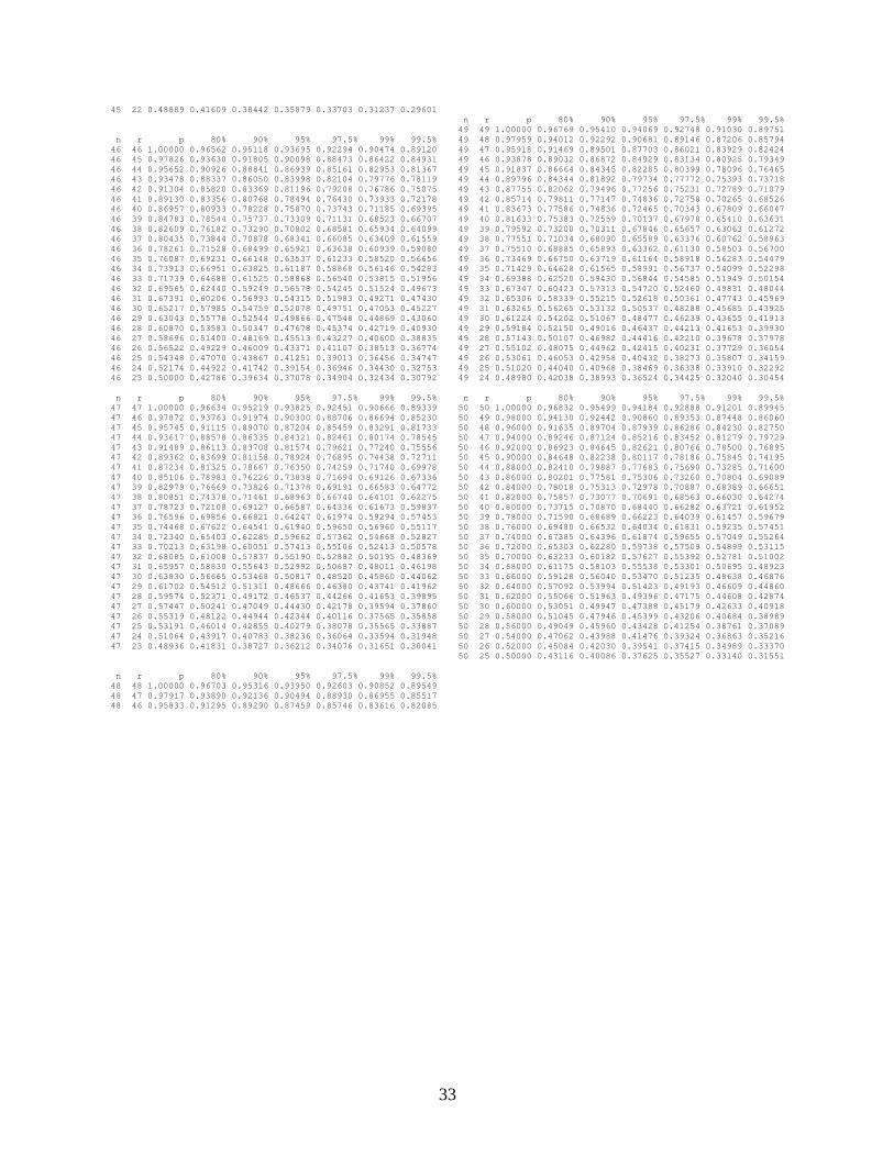
33

45 22 0.48889 0.41609 0.38442 0.35879 0.33703 0.31237 0.29601 n r p 80% 90% 95% 97.5% 99% 99.5% 49 49 1.00000 0.96769 0.95410 0.94069 0.92748 0.91030 0.89751 n r p 80% 90% 95% 97.5% 99% 99.5% 49 48 0.97959 0.94012 0.92292 0.90681 0.89146 0.87206 0.85794 46 46 1.00000 0.96562 0.95118 0.93695 0.92294 0.90474 0.89120 49 47 0.95918 0.91469 0.89501 0.87703 0.86021 0.83929 0.82424 46 45 0.97826 0.93630 0.91805 0.90098 0.88473 0.86422 0.84931 49 46 0.93878 0.89032 0.86872 0.84929 0.83134 0.80925 0.79349 46 44 0.95652 0.90926 0.88841 0.86939 0.85161 0.82953 0.81367 49 45 0.91837 0.86664 0.84345 0.82285 0.80399 0.78096 0.76465 46 43 0.93478 0.88337 0.86050 0.83998 0.82104 0.79776 0.78119 49 44 0.89796 0.84344 0.81892 0.79734 0.77772 0.75393 0.73718 46 42 0.91304 0.85820 0.83369 0.81196 0.79208 0.76786 0.75075 49 43 0.87755 0.82062 0.79496 0.77256 0.75231 0.72789 0.71079 46 41 0.89130 0.83356 0.80768 0.78494 0.76430 0.73933 0.72178 49 42 0.85714 0.79811 0.77147 0.74836 0.72758 0.70265 0.68526 46 40 0.86957 0.80933 0.78228 0.75870 0.73743 0.71185 0.69395 49 41 0.83673 0.77586 0.74836 0.72465 0.70343 0.67809 0.66047 46 39 0.84783 0.78544 0.75737 0.73309 0.71131 0.68523 0.66707 49 40 0.81633 0.75383 0.72559 0.70137 0.67978 0.65410 0.63631 46 38 0.82609 0.76182 0.73290 0.70802 0.68581 0.65934 0.64099 49 39 0.79592 0.73200 0.70311 0.67846 0.65657 0.63063 0.61272 46 37 0.80435 0.73844 0.70878 0.68341 0.66085 0.63409 0.61559 49 38 0.77551 0.71034 0.68090 0.65589 0.63376 0.60762 0.58963 46 36 0.78261 0.71528 0.68499 0.65921 0.63638 0.60939 0.59080 49 37 0.75510 0.68885 0.65893 0.63362 0.61130 0.58503 0.56700 46 35 0.76087 0.69231 0.66148 0.63537 0.61233 0.58520 0.56656 49 36 0.73469 0.66750 0.63719 0.61164 0.58918 0.56283 0.54479 46 34 0.73913 0.66951 0.63825 0.61187 0.58868 0.56146 0.54283 49 35 0.71429 0.64628 0.61565 0.58991 0.56737 0.54099 0.52298 46 33 0.71739 0.64688 0.61525 0.58868 0.56540 0.53815 0.51956 49 34 0.69388 0.62520 0.59430 0.56844 0.54585 0.51949 0.50154 46 32 0.69565 0.62440 0.59249 0.56578 0.54245 0.51524 0.49673 49 33 0.67347 0.60423 0.57313 0.54720 0.52460 0.49831 0.48044 46 31 0.67391 0.60206 0.56993 0.54315 0.51983 0.49271 0.47430 49 32 0.65306 0.58339 0.55215 0.52618 0.50361 0.47743 0.45969 46 30 0.65217 0.57985 0.54759 0.52078 0.49751 0.47053 0.45227 49 31 0.63265 0.56265 0.53132 0.50537 0.48288 0.45685 0.43925 46 29 0.63043 0.55778 0.52544 0.49866 0.47548 0.44869 0.43060 49 30 0.61224 0.54202 0.51067 0.48477 0.46239 0.43655 0.41913 46 28 0.60870 0.53583 0.50347 0.47678 0.45374 0.42719 0.40930 49 29 0.59184 0.52150 0.49016 0.46437 0.44213 0.41653 0.39930 46 27 0.58696 0.51400 0.48169 0.45513 0.43227 0.40600 0.38835 49 28 0.57143 0.50107 0.46982 0.44416 0.42210 0.39678 0.37978 46 26 0.56522 0.49229 0.46009 0.43371 0.41107 0.38513 0.36774 49 27 0.55102 0.48075 0.44962 0.42415 0.40231 0.37729 0.36054 46 25 0.54348 0.47070 0.43867 0.41251 0.39013 0.36456 0.34747 49 26 0.53061 0.46053 0.42958 0.40432 0.38273 0.35807 0.34159 46 24 0.52174 0.44922 0.41742 0.39154 0.36946 0.34430 0.32753 49 25 0.51020 0.44040 0.40968 0.38469 0.36338 0.33910 0.32292 46 23 0.50000 0.42786 0.39634 0.37078 0.34904 0.32434 0.30792 49 24 0.48980 0.42038 0.38993 0.36524 0.34425 0.32040 0.30454 n r p 80% 90% 95% 97.5% 99% 99.5% n r p 80% 90% 95% 97.5% 99% 99.5% 47 47 1.00000 0.96634 0.95219 0.93825 0.92451 0.90666 0.89339 50 50 1.00000 0.96832 0.95499 0.94184 0.92888 0.91201 0.89945 47 46 0.97872 0.93763 0.91974 0.90300 0.88706 0.86694 0.85230 50 49 0.98000 0.94130 0.92442 0.90860 0.89353 0.87448 0.86060 47 45 0.95745 0.91115 0.89070 0.87204 0.85459 0.83291 0.81733 50 48 0.96000 0.91635 0.89704 0.87939 0.86286 0.84230 0.82750 47 44 0.93617 0.88578 0.86335 0.84321 0.82461 0.80174 0.78545 50 47 0.94000 0.89246 0.87124 0.85216 0.83452 0.81279 0.79729 47 43 0.91489 0.86113 0.83708 0.81574 0.79621 0.77240 0.75556 50 46 0.92000 0.86923 0.84645 0.82621 0.80766 0.78500 0.76895 47 42 0.89362 0.83699 0.81158 0.78924 0.76895 0.74438 0.72711 50 45 0.90000 0.84648 0.82238 0.80117 0.78186 0.75845 0.74195 47 41 0.87234 0.81325 0.78667 0.76350 0.74259 0.71740 0.69978 50 44 0.88000 0.82410 0.79887 0.77683 0.75690 0.73285 0.71600 47 40 0.85106 0.78983 0.76226 0.73838 0.71694 0.69126 0.67336 50 43 0.86000 0.80201 0.77581 0.75306 0.73260 0.70804 0.69089 47 39 0.82979 0.76669 0.73826 0.71378 0.69191 0.66583 0.64772 50 42 0.84000 0.78018 0.75313 0.72978 0.70887 0.68389 0.66651 47 38 0.80851 0.74378 0.71461 0.68963 0.66740 0.64101 0.62275 50 41 0.82000 0.75857 0.73077 0.70691 0.68563 0.66030 0.64274 47 37 0.78723 0.72108 0.69127 0.66587 0.64336 0.61673 0.59837 50 40 0.80000 0.73715 0.70870 0.68440 0.66282 0.63721 0.61952 47 36 0.76596 0.69856 0.66821 0.64247 0.61974 0.59294 0.57453 50 39 0.78000 0.71590 0.68689 0.66223 0.64039 0.61457 0.59679 47 35 0.74468 0.67622 0.64541 0.61940 0.59650 0.56960 0.55117 50 38 0.76000 0.69480 0.66532 0.64034 0.61831 0.59235 0.57451 47 34 0.72340 0.65403 0.62285 0.59662 0.57362 0.54668 0.52827 50 37 0.74000 0.67385 0.64396 0.61874 0.59655 0.57049 0.55264 47 33 0.70213 0.63198 0.60051 0.57413 0.55106 0.52413 0.50578 50 36 0.72000 0.65303 0.62280 0.59738 0.57509 0.54899 0.53115 47 32 0.68085 0.61008 0.57837 0.55190 0.52882 0.50195 0.48369 50 35 0.70000 0.63233 0.60182 0.57627 0.55392 0.52781 0.51002 47 31 0.65957 0.58830 0.55643 0.52992 0.50687 0.48011 0.46198 50 34 0.68000 0.61175 0.58103 0.55538 0.53301 0.50695 0.48923 47 30 0.63830 0.56665 0.53468 0.50817 0.48520 0.45860 0.44062 50 33 0.66000 0.59128 0.56040 0.53470 0.51235 0.48638 0.46876 47 29 0.61702 0.54512 0.51311 0.48666 0.46380 0.43741 0.41962 50 32 0.64000 0.57092 0.53994 0.51423 0.49193 0.46609 0.44860 47 28 0.59574 0.52371 0.49172 0.46537 0.44266 0.41653 0.39895 50 31 0.62000 0.55066 0.51963 0.49396 0.47175 0.44608 0.42874 47 27 0.57447 0.50241 0.47049 0.44430 0.42178 0.39594 0.37860 50 30 0.60000 0.53051 0.49947 0.47388 0.45179 0.42633 0.40918 47 26 0.55319 0.48122 0.44944 0.42344 0.40116 0.37565 0.35858 50 29 0.58000 0.51045 0.47946 0.45399 0.43206 0.40684 0.38989 47 25 0.53191 0.46014 0.42855 0.40279 0.38078 0.35565 0.33887 50 28 0.56000 0.49049 0.45960 0.43428 0.41254 0.38761 0.37089 47 24 0.51064 0.43917 0.40783 0.38236 0.36064 0.33594 0.31948 50 27 0.54000 0.47062 0.43988 0.41476 0.39324 0.36863 0.35216 47 23 0.48936 0.41831 0.38727 0.36212 0.34076 0.31651 0.30041 50 26 0.52000 0.45084 0.42030 0.39541 0.37415 0.34989 0.33370 50 25 0.50000 0.43116 0.40086 0.37625 0.35527 0.33140 0.31551 n r p 80% 90% 95% 97.5% 99% 99.5% 48 48 1.00000 0.96703 0.95316 0.93950 0.92603 0.90852 0.89549 48 47 0.97917 0.93890 0.92136 0.90494 0.88930 0.86955 0.85517 48 46 0.95833 0.91295 0.89290 0.87459 0.85746 0.83616 0.82085

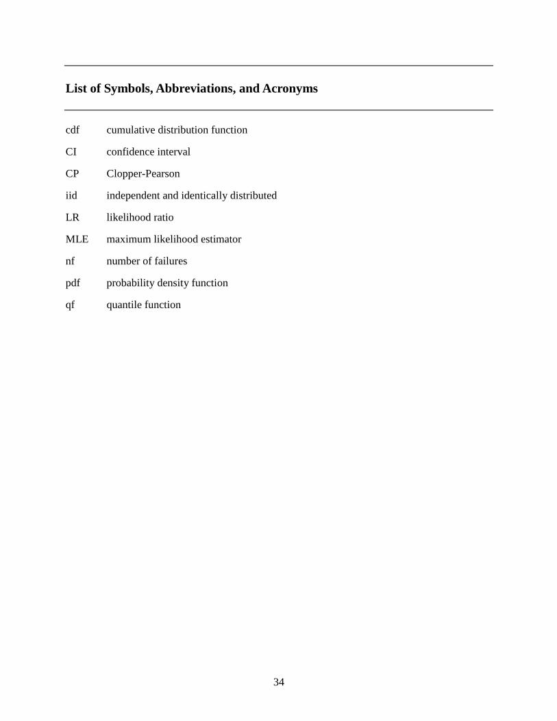
34

List of Symbols, Abbreviations, and Acronyms

cdf cumulative distribution function

CI confidence interval

CP Clopper-Pearson

iid independent and identically distributed

LR likelihood ratio

MLE maximum likelihood estimator

nf number of failures

pdf probability density function

qf quantile function

NO. OF COPIES ORGANIZATION

35

1 DEFENSE TECHNICAL (PDF INFORMATION CTR only) DTIC OCA 8725 JOHN J KINGMAN RD STE 0944 FORT BELVOIR VA 22060-6218 1 DIRECTOR US ARMY RESEARCH LAB IMNE ALC HRR 2800 POWDER MILL RD ADELPHI MD 20783-1197 1 DIRECTOR US ARMY RESEARCH LAB RDRL CIM L 2800 POWDER MILL RD ADELPHI MD 20783-1197 1 DIRECTOR US ARMY RESEARCH LAB RDRL CIM P 2800 POWDER MILL RD ADELPHI MD 20783-1197 1 ASST SECY ARMY (CD ACQSTN LOGISTICS & TECH only) SAAL ZP RM 2E661 103 ARMY PENTAGON WASHINGTON DC 20310-0103 1 ASST SECY ARMY (CD ACQSTN LOGISTICS & TECH only) SAAL ZS RM 3E448 103 ARMY PENTAGON WASHINGTON DC 20310-0103 1 DIRECTOR FORCE DEV (CD DAPR FDZ only) RM 3A522 460 ARMY PENTAGON WASHINGTON DC 20310-0460 1 US ARMY TRADOC ANL CTR ATRC W A KEINTZ WSMR NM 88002-5502 1 USARL RDRL SLE R FLORES WSMR NM 88002-5513

ABERDEEN PROVING GROUND 1 US ARMY DEV TEST COM CSTE DTC TT T 314 LONGS CORNER RD APG MD 21005-5055 1 US ARMY EVALUATION CTR CSTE AEC SVE R LAUGHMAN 4120 SUSQUEHANNA AVE APG MD 21005-3013 22 DIR USARL RDRL SL J BEILFUSS J FEENEY J FRANZ M STARKS P TANENBAUM RDRL SLB G MANNIX RDRL SLB A D FARENWALD RDRL SLB D R GROTE RDRL SLB E M PERRY RDRL SLB G P MERGLER RDRL SLB S S SNEAD RDRL SLB W L ROACH RDRL CIM G (BLDG 4600) RDRL SLB D J COLLINS (5 CPS) J EDWARDS T HOLDREN L MOSS E SNYDER