Bill.Shipley@USherbrooke.ca

Community assembly through trait selection

(CATS):Modelling from

incomplete information

A seminar in three parts

The ecological concept

The maximum entropy formalism

Edwin Jaynes

The CATS model

Part 1

The ecological concept

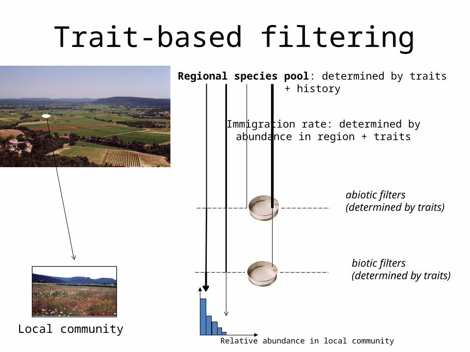
Trait-based filteringRegional species pool: determined by traits + history

abiotic filters (determined by traits)

biotic filters(determined by traits)

Immigration rate: determined by abundance in region + traits

Local communityRelative abundance in local community

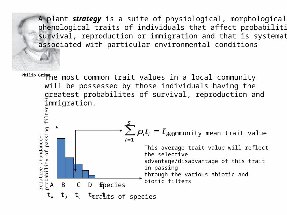
Philip Grime

A plant strategy is a suite of physiological, morphological or phenological traits of individuals that affect probabilities ofsurvival, reproduction or immigration and that is systematicallyassociated with particular environmental conditions

The most common trait values in a local community will be possessed by those individuals having the greatest probabilites of survival, reproduction and immigration.

rela

tive

ab

un

da

nce

~p

rob

ab

ility

of

pa

ssin

g f

ilte

rs

A B C D E species

tA tB tC td tE traits of species

This average trait value will reflect the selectiveadvantage/disadvantage of this trait in passingthrough the various abiotic and biotic filters

∑1=

=S

iwmii ttp community mean trait value

Philip Grime

Two consequences of Grime’s ideasfor community assembly…

1. If we know the values of particular abiotic variables determining the filters, then we should be able to predict the « typical » values of

the functional traits found in this local community; i.e. community-weighted means.

2. If we know the « typical » values of the functional traits that are found in this community, and we know the actual trait values of the species in a regional species pool, then we should be able to predict which of these species will be dominants, which will be subordinates, and which will be rare or absent.

The three basic parts of the CATS model

λ: selection on trait in the local community(greater probability of passing if smaller…)

q : distribution of relative abundance of species in themetacommunity

metacommunity

Trait (t)

p : distribution of relative abundance of species in thelocal community

Trait (t)

Grimes’s plant strategy

metacommunity

Local community

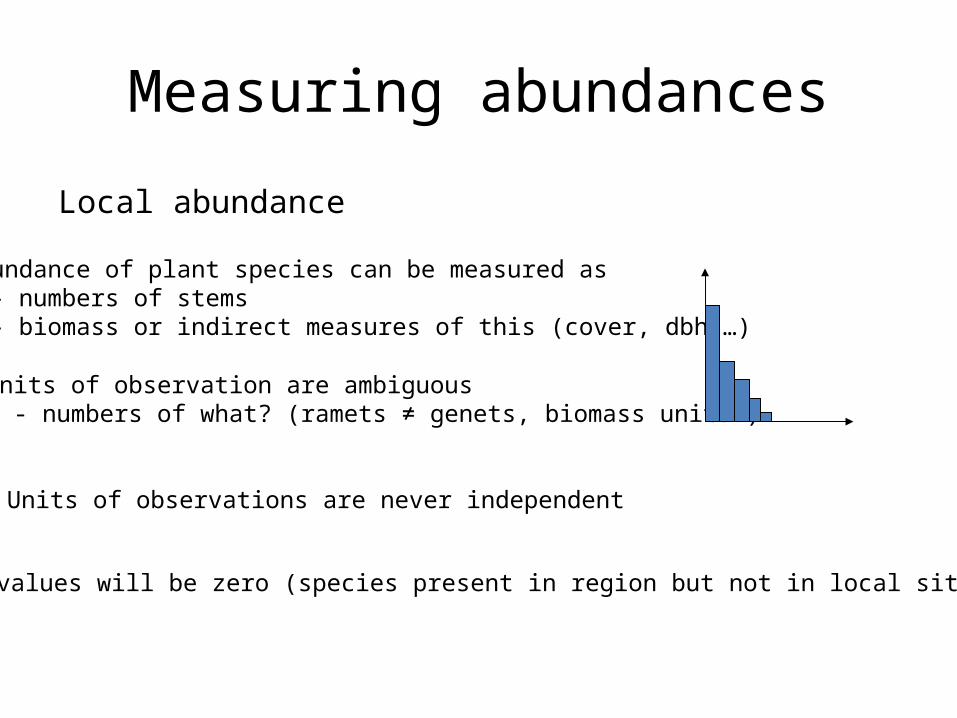
Measuring abundances

Abundance of plant species can be measured as - numbers of stems - biomass or indirect measures of this (cover, dbh …)

Units of observation are ambiguous - numbers of what? (ramets ≠ genets, biomass units?)

Units of observations are never independent

Local abundance

Most values will be zero (species present in region but not in local site)

Measuring abundances

Meta-community abundances

Sometimes no information

Sometimes vague information (very common, common, rare)

Sometimes more quantitative information

Part 2

The maximum entropy formalismEdwin Jaynes

Jaynes, E.T. 2003. Probability theory. The logic of science. Cambridge U Press.

How can we quantify learning?If the sun does set tonight (and our previous information told us it would, p=0.99999) then we will have learned almost nothing new (almost no new information)

If the sun doesn’t set tonight (and our previous information told us it would, 1-p=0.00001) then we will have learned something incredible (lots of new information)

The amount of learning (new information):Historical log2, we will use loge=ln

Claude Shannon

I=l𝑛( 1𝑝 )=−l𝑛 (𝑝)

Average information content (i.e. new information)

Specify all of the logically possible states in which some phenomenon can exist (i=1,2,…,S)

Based on what we know before observing the actual state, assign values between 0 and 1 to each possible state: p=(p1, p2, …, pS)

1 1 1

ln lnS S S

i i i i i ii i i

I p I p p p p

Information entropy

The amount of new information that we will learn if state i occurs is 𝐼 𝑖=− 𝑙𝑛𝑝𝑖

1

S

i ii

I p I

The average amount of new information that we will learn is

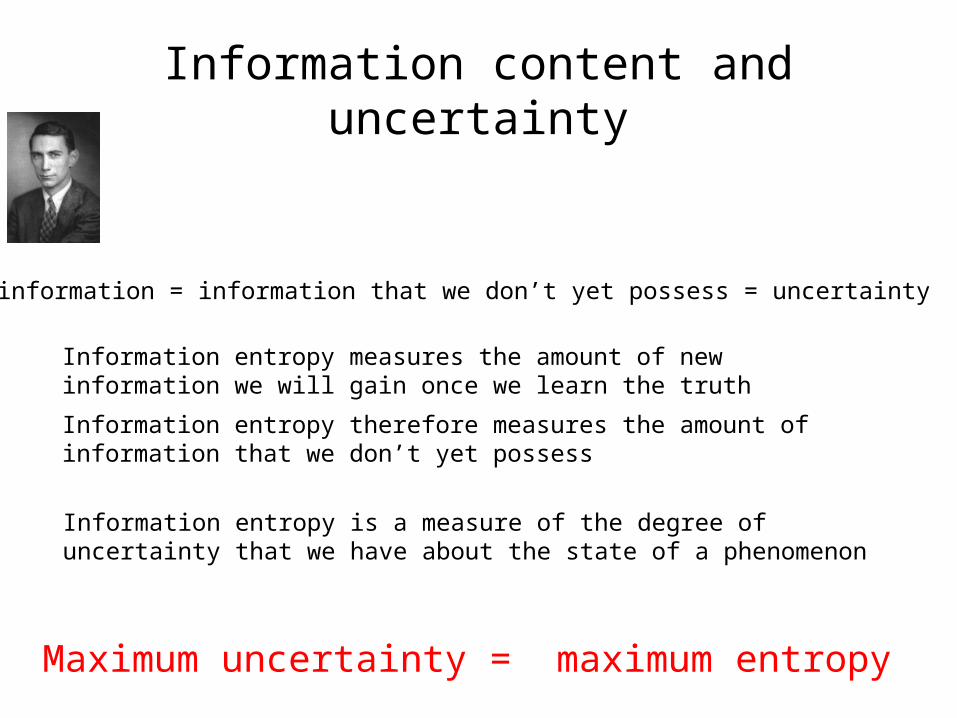
Information content and uncertainty

New information = information that we don’t yet possess = uncertainty

Information entropy measures the amount of new information we will gain once we learn the truth

Information entropy therefore measures the amount of information that we don’t yet possess

Information entropy is a measure of the degree of uncertainty that we have about the state of a phenomenon

Maximum uncertainty = maximum entropy

A betting game: game A

I bring you, blindfolded, to a field outside Sherbrooke.

I tell you that there is a plant at your feet that belongs to either species A or species B.

You have assign probabilities to the two possible states (species A or B) and will get that proportion of $1,000,000 once you learn the species name.

What is your answer?

1

ln (0.5ln(0.5) 0.5ln 0.5 ) 0.69S

i ii

I p p

A betting game: game B

New game with some new clues:

(i) The site is a former cultivated field that was abandoned by a farmer last year.(ii) Species A is an annual herb. Species B is a climax tree.

You have assign probabilities to the two possible states and will get that proportion of $1,000,000.

What is your answer?

If you changed your bet in this second game then these new clues provided you with some new, but incomplete, information before you learned the answer.

1

ln (0.9 ln(0.9) 0.1ln 0.1 ) 0.33S

i ii

I p p

0.0 0.2 0.4 0.6 0.8 1.0

0.1

0.2

0.3

0.4

0.5

0.6

0.7

p(species A)

en

tro

py

Maximum entropy (maximum uncertainty) at p=(0.5,0.5)

p(annual herb)=0.9p(climax tree)=0.1)

Amount of information contained in the ecological clues

Amount of remaining uncertianty, given the ecological clues

Relative entropy (Kullback-Leibler divergence)

Let qi=1/S and S be the fixed number of unordered, discrete states; q is a uniform distribution

Relative to a “prior” or reference distribution (q)−∑ 𝑝𝑖 ln(𝑝𝑖

𝑞𝑖)

−∑ 𝑝𝑖 ln( 𝑝𝑖

( 1𝑆 ) )=−∑ 𝑝𝑖 (ln𝑝𝑖+ ln𝑆 )=−∑ 𝑝𝑖 ln𝑝𝑖+constant

Information entropy α relative entropy given a uniform distribution

Maximizing relative entropy = maximizing entropy

The maximum entropy formalism in an ecological context: A three-step program

Edwin Jaynes

Jaynes, E.T. 2003. Probability theory. The logic of science. Cambridge U

Press.

The maximum entropy formalism in an ecological contextEdwin Jaynes

Jaynes, E.T. 2003. Probability theory. The logic of science. Cambridge U

Press.

Specify a reference (q, prior) distribution that encodes what you know about the relative abundances of each species in the species pool before obtaining any information about the local community.

Step 1: specifying the relative abundances in the regional meta-community (the prior distribution)

“All I know is that there are S species in the meta-community” 𝑞𝑖=1𝑆

“All I know is that there are S species in the meta-community and I know their relative abundances in this meta-community”

qi

The maximum entropy formalism in an ecological contextEdwin Jaynes

Jaynes, E.T. 2003. Probability theory. The logic of science. Cambridge U

Press.

Step 2: quantifying what we know about trait-based community assembly in the local community

“I have measured the average value of my functional traits(community-weighted traits values)”

“ I have measured the environmental conditions, and know the function linking these environmental conditions to the community-weighted trait values”

𝑡1=23.3𝑡 2=147.1𝑒𝑡𝑐 .

2 4 6 8 10

12

34

56

xy

y=2.5+0.23x

The maximum entropy formalism in an ecological contextEdwin Jaynes

Jaynes, E.T. 2003. Probability theory. The logic of science. Cambridge U

Press.

Step 3: choose a probability distribution which agrees with what we know, but doesn’t include any more information (i.e. don’t lie).

−∑ 𝑝𝑖 ln(𝑝𝑖

𝑞𝑖)

Choose values of p that agree with what we know:𝑞 ,∑

𝑖=1

𝑆

𝑝𝑖

𝑡1=∑𝑖=1

𝑆

𝑝𝑖 𝑡𝑖1=¿23.3¿𝑡 2=∑𝑖=1

𝑆

𝑝𝑖 𝑡 21=¿147.1¿𝑒𝑡𝑐 .

And that maximizes the remaining uncertainty

The maximum entropy formalism in an ecological contextEdwin Jaynes

Jaynes, E.T. 2003. Probability theory. The logic of science. Cambridge U

Press.

The solution is a general exponential distribution

𝑝𝑖=𝑞𝑖𝑒

−∑𝑗=1

𝑇

𝜆 𝑗 𝑡𝑖𝑗

∑𝑖=1

𝑆

𝑞𝑖𝑒−∑

𝑗=1

𝑇

𝜆 𝑗 𝑡 𝑖𝑗

tij: Trait value of trait j of species iqi: Prior distribution of species i

λj:The amount by which a one-unit increase in trait j will result in a proportional change in relative abundance (pi)

The maximum entropy formalism in an ecological contextEdwin Jaynes

Jaynes, E.T. 2003. Probability theory. The logic of science. Cambridge U

Press.

Practical considerations

Except for maxent models with only a few constraints, we need numerical methods in order to fit them to data. I use a proportionality between the maximum likelihood of a multinomial distribution and the λ values of the solution to the maxent problem (Improved Iterative Scaling), available in the maxent() function of the FD library in R.Della Pietra, S. Della Pietra, V., Lafferty, J. 1997. Inducing features of random fields. IEEE Transactions Patern Analysis and Machine Intelligence 19:1-13

Laliberté, E., Shipley, B. 2009. Measuring functional diversity from multiple traits, and other tools for functional ecology R. package, Vienna, Austria

By permuting trait vectors relative to species’ observed relative abundances, one can develop permutation tests of significance concerning model fit

Shipley, B. 2010. Ecology 91:2794-2805

There are now many empirical applications of this model in many places around the world, and applied at many geographical scales.

Two examples…

CATS

96 1m2 quadrats containing the understory herbaceous plants of ponderosa pine forests (Arizona USA).Quadrats were distributed across seven permanent sites within a 120 km2 landscape between 2000-2500 m altitude.

SHIPLEY et al. 2011. A strong test of a maximum entropy model of trait-based community assembly. Ecology 92: 507–517.

Daniel Laughlin’s PhD thesis

Available information

12 environmental variables measured in each quadrat

20 functional traits measured per species

Relative abundance of each species in each quadrat

Significant predictive ability by 3 traits

After ~7 traits, mostly redundant information

0.0 0.2 0.4 0.6 0.8 1.0

0.0

0.2

0.4

0.6

0.8

1.0

Observed relative abundance

Pre

dic

ted

re

lativ

e a

bun

da

nce

r= 0.97

1e-04 1e-02 1e+00

1e

-04

1e

-03

1e

-02

1e

-01

1e

+00

Observed relative abundance

Pre

dic

ted

re

lativ

e a

bun

da

nce

r= 0.58

If species is present, and not rare (>10%), CATS predicts its abundance well

If species is present, but rare (<10%), CATS can’t distinguish degrees of rarity

If species is absent (X) then CATS will predict it to be rare

If we only know the environmental conditions of a site, and the general relationship between community-weighted traits and the environment, how well can CATS do?

2 4 6 8 10

24

68

environment X

CW

M tr

ait

Actual measured community-weighted value for this site = 9.5

General relationship: Y=2.5+0.73X

Predicted value for community-weighted trait, given that we know the environmental value is 7 = 7.61

0 2 4 6 8 10

51

01

52

02

5

environment X

Ab

un

da

nce

of s

pe

cie

s S

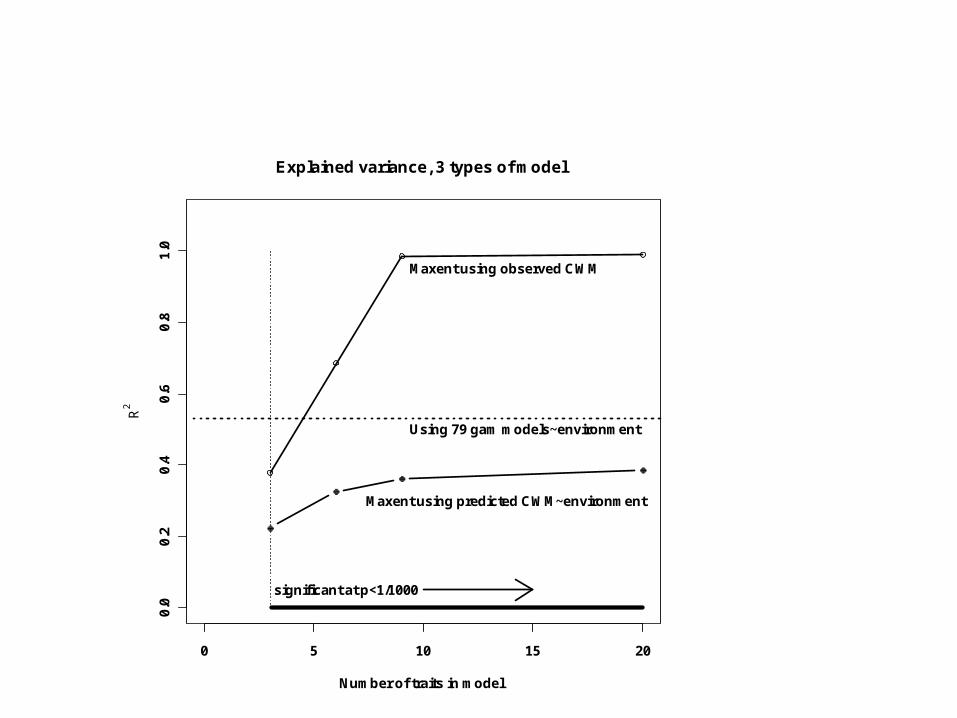
The best possible prediction given the environment would be obtained with 79 separate generalized additive (form-free) regressions – one for each species in the species pool – of relative abundance vs. the environmental variables.

gam(S~X)

0 5 10 15 20

0.0

0.2

0.4

0.6

0.8

1.0

Number of traits in model

R2

Explained variance, 3 types of model

Maxent using predicted CWM~environment

Maxent using observed CWM

Using 79 gam models~environment

significant at p<1/1000

Shipley, Paine & Baraloto. 2012. Quantifying the importance of local niche-based and stochastic processes to tropical tree community assembly. . Ecology 93: 760-769

Stephen Hubbell

The unified neutral theory of biodiversity and biogeography

The per capita probabilities of immigration from the meta-community, andthe per capita probabilities of survival and reproduction of all species areequal (demographic neutrality).

Subsequent population dynamics in the local community are determined purely by random drift.

Local relative abundance ~meta-community relative abundance + drift

« Neutral prior » = meta-community relative abundances

Second example: tropical forests in French Guiana

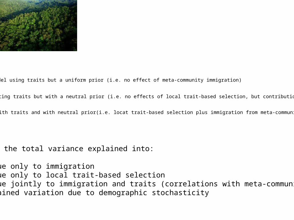
1. Fit model using traits but a uniform prior (i.e. no effect of meta-community immigration)

2. Fit model permuting traits but with a neutral prior (i.e. no effects of local trait-based selection, but contribution from immigration)

3. Fit model with traits and with neutral prior(i.e. locat trait-based selection plus immigration from meta-community

Partition the total variance explained into:

1. That due only to immigration2. That due only to local trait-based selection3. That due jointly to immigration and traits (correlations with meta-community4. Unexplained variation due to demographic stochasticity

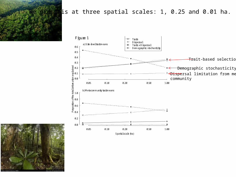
0.05 0.10 0.20 0.50 1.00

0.0

0.1

0.2

0.3

0.4

0.5

0.6a) Site-level trait means

TraitsDispersalTraits x DispersalDemographic stochasticity

0.05 0.10 0.20 0.50 1.00

0.0

0.2

0.4

0.6

0.8

1.0

Spatial scale (ha)

Pro

porti

on o

f the

tota

l inf

orm

atio

n ex

plai

ned

b) Metacommunity trait means

Figure 1

We did this at three spatial scales: 1, 0.25 and 0.01 ha.

Dispersal limitation from meta-community

Trait-based selection

Demographic stochasticity

http://www.amazon.co.uk/gp/reader/0521133556/ref=sib_dp_pt

Practical considerations. How do we fit this model to empirical data? A trick involving likelihood

1

1

!; , , ,q

!

i

Sai i iS

ii

i

AP A p

a

a p λ T

the number of independent allocations to species i

A total of A independent allocations of individuals or units of biomass into each of the S species in the species pool

The probability of a single allocation going to species i (i.e. the probability of sufficient resources being captured to produce one individual or unit of biomass for species i); a function of its traits (Ti), the strength of the trait on selection (λ), and its meta-community abundance (qi)

1 1

1

!( ; ) ( , , ) ( , , )

!

i i

S Sa ai i i ik i iS

i ii

i

AA p C p

a

p a, λ T q λ T qLThe likelihood:

Taking logarithms, dividing both sides by A, and re-arranging, one obtains

1 1

ln ; , ln( )ln , , ln , ,

S Si

i i i i i i ii i

a A C ap o p

A A

pλ T q λ T q

L

In practice we can never know this, since neither individuals or resources (biomass) are ever allocated independently…

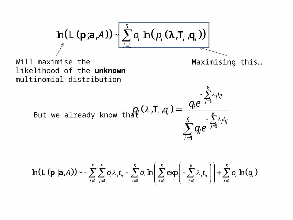
1

ln ; , ~ ln , ,S

i i i ii

A o pp a λ T qL

Maximising this…Will maximise the likelihood of the unknown multinomial distribution

1

1

1

, ,

k

j ijj

i i k

j ijj

t

ii

tS

ii

qq e

p

q e

TBut we already know that

1 1 1 1 1 1

ln | , ~ ln exp lnS k S S k S

i j ij i j ij i ii j i i j i

A o t o t o q

p aL

1 1 1 1 1 1

ln | , ~ ln exp lnS k S S k S

i j ij i j ij i ii j i i j i

A o t o t o q

p aL

Choose values of λ that maximise this function, given the vector of traits (ti) for each species in the species pool and their meta-community abundances (qi):

The dual solution (Della Pietra et al. 1997): the values of λ that maximise the relative entropy in the maximum entropy formalism are the same as the values that maximise the likelihood of a multinomial distribution.

Della Pietra, S. Della Pietra, V., Lafferty, J. 1997. Inducing features of random fields. IEEE Transactions Patern Analysis and Machine Intelligence 19:1-13.

Improved Iterative Scaling algorithm maxent() in the FD package of R.

Laliberté, E., Shipley, B. 2009. Measuring functional diversity from multiple traits, and other tools for functional ecology R. package, Vienna, Austria

Permutation tests for the CATS model

Choose values of p that agree with what we know:

𝑞 ,∑𝑖=1

𝑆

𝑝𝑖

𝑡 j=∑𝑖=1

𝑆

𝑝𝑖 𝑡𝑖 j=¿¿

¿−∑ 𝑝𝑖 ln(𝑝𝑖

𝑞𝑖)And that maximizes the

remaining uncertainty

H0: trait values (tij) are independent of the observed relative abundances (oi)

2. Randomly permute the vector of trait values (T*i) between the species

(so traits are independent of observed relative abundances)

3. Calculate * *

1

ln ,S

i i i ii

f o p T q

o,p,q , q

4. Repeat steps 2 & 3 a large number of times.

1. Calculate 1

ln ,S

i i i ii

f o p q

o,p,q ,T q The smaller the value, the better the fit

5. Count the number of times f*> f. This is an estimate of the null probability.

Permutation tests for the CATS model

maxent.test() function in the FD library.

Shipley, B. 2010. Ecology 91:2794-2805