
Big
189
7/17/2019 Big http://slidepdf.com/reader/full/big563db8d5550346aa9a975e13 1/189 . Advanced CFD Modelling of Road-Vehicle Aerodynamics A thesis submitted to the University of Manchester Institute of Science and Technology for the degree of Doctor of Philosophy May 2001 Christopher M.E. Robinson Department of Mechanical, Aerospace and Manufacturing Engineering
-
Upload
junaidmasoodi -
Category
Documents
-
view
4 -
download
0
description
big
Transcript of Big

7/17/2019 Big
http://slidepdf.com/reader/full/big563db8d5550346aa9a975e13 1/189
.
Advanced CFD Modelling of Road-Vehicle Aerodynamics
A thesis submitted to the University of Manchester
Institute of Science and Technology for the degree of
Doctor of Philosophy
May 2001
Christopher M.E. Robinson
Department of Mechanical,
Aerospace and Manufacturing Engineering

7/17/2019 Big
http://slidepdf.com/reader/full/big563db8d5550346aa9a975e13 2/189
Declaration
No portion of the work referred to in this thesis has been submitted in support of an applica-
tion for another degree or qualification of this or any other university, or other institution of
learning.
ii
7/17/2019 Big
http://slidepdf.com/reader/full/big563db8d5550346aa9a975e13 3/189
Acknowledgements
I would like to express my sincere gratitude to Professor B.E. Launder, my supervisor,
for his invaluable advice, guidance and constructive criticism throughout the course of this
research. I am honoured to have been given this opportunity to work in his research group.
I would also like to thank Dr T.J. Craft and Dr H. Iacovides for their continuous help
and advice. The many discussions I have had with them have benefitted considerably my
understanding of turbulent flows and turbulence modelling.
Funding for this project was provided by the European Union BRITE/EURAM Project
BE-97-4043: Models for Vehicle Aerodynamics (MOVA). Without this support, the present
study would not have been possible. I would like to thank all the members of the MOVA
project group for their advice on turbulence modelling and experiments, and the insight to
industrial applications of turbulence modelling which they have provided. In particular I
would like to thank: Professor D. Laurence (UMIST & Electricité de France), Professor K.
Hanjalic (TU Delft), Dr H. Lienhart (LSTM, Erlangen), Dr L. Elena (PSA, Peugeot-Citroën)
and Dr B. Basara (AVL, Graz).
My thanks to friends and colleagues at UMIST for providing advice, discussion, enter-
tainment and coffee - thanks to all members of the TM & CFD Group, especially: Simon
Gant, Aleksey Gerasimov and Dr Rob Prosser. Also, very special thanks go to my friends:
Dougie & Sharon, Martin, Ajay & Kerry and Simon for their support and encouragement,and providing me with many much-needed distractions.
Last, but by no means least, I would like to thank Mum, Dad, Tim & Jo, without whose
love, none of this would be possible.
iii
7/17/2019 Big
http://slidepdf.com/reader/full/big563db8d5550346aa9a975e13 4/189
Abstract
This thesis is concerned with the application of a cubic non-linear k ε model to flows per-
tinent to road-vehicle aerodynamics. Three simple test cases are initially considered and a
simplified car model - the Ahmed body - is used as a final test case. The performance of the
non-linear k ε model is compared to a linear k ε model and, for one test case, a realizable
differential stress model. As the principal thrust of the work is to mimic current industrial
practices, wall functions are used to bridge the near-wall flow. Both established log-law wall
functions and a new analytical wall function are used.
The three simple test cases are: flow around a cylinder of square cross-section placed near
a wall, flow in a U-bend of square cross-section and flow in a plane diffuser. In calculating
the flow around the square cross-sectioned cylinder, the non-linear k ε model performs
generally better than the linear k ε model. In the case with a steady wake (g
d 0
25; Re
13 600) both the non-linear model and the linear model calculate too long a recirculating flow
region behind the cylinder. The linear model calculates velocity profiles in the wake more
accurately but the non-linear model calculates the Reynolds stresses better. Flow with vortexshedding in the wake has also been calculated (g
d 0
50 and 0.75).
In the square cross-sectioned U-bend, the non-linear k ε model is compared with a
differential stress model. This case allows comparison of the models in a flow with strong
streamline curvature and streamwise vorticity. The radius of curvature of the bend is Rc
D
3 35 and the Reynolds number of the flow is Re
58
000; there is no separation of the flow.
The non-linear k ε model calculates the mean velocities almost as well as the differential
stress model. It calculates the low momentum region in the central part of the duct well
and also the complex secondary flow pattern in the U-bend. The Reynolds stresses are not
calculated as well by the non-linear k ε model as they are by the differential stress model,
because the non-linear k ε model calculates these from local velocity gradients rather than
transport equations.
The plane diffuser is used to test both the cubic non-linear k ε model and the new ana-
lytical wall function. The flow is calculated at Re 20 000, the diffuser has one 10o inclined
wall and separation occurs part way along this wall. When the analytical wall function is used
iv

7/17/2019 Big
http://slidepdf.com/reader/full/big563db8d5550346aa9a975e13 5/189
v
in conjunction with a linear k ε model, a small amount of separation is calculated. A linear
k ε model with a log-law wall function calculates no separation. The flow calculation is
improved further by the non-linear k ε model; the most accurate combination of turbulence
model and wall function tested for this case is the non-linear k ε model and analytical wall
function.The final test case is flow around a simplified car geometry - the Ahmed body - which
is a commonly used test case in industry. The Ahmed body is a bluff body mounted near a
ground-plane; the most significant feature of the body is the angle of the rear slant. Below a
critical angle (30o , the flow over the rear slant is predominantly attached and is characterised
by high drag and the formation of strong vortices at the side edges of the slant. Above the
critical angle, the flow is completely separated, there is relatively low drag and only weak
side-edge vortices form. Calculations of the flow are made for the Ahmed body with two
rear-slant angles which bracket the critical angle (25o and 35o).
For the body with the 25o rear-slant, the linear k ε model calculates the attached flow
with the strong side-edge vortices reasonably well; the non-linear k ε model does not cal-
culate this flow well. Only weak side-edge vortices are calculated by the non-linear model
which do not draw enough fluid out of the boundary layer over the slant to cause the flow
to attach. The influence of the choice of wall function, time-dependent effects, realizability,
near-wall length-scale correction, convection scheme, development of streamwise vorticity
and sensitivity to features of the non-linear k ε model are discussed. Over the 35o rear slant
both the linear and non-linear k ε models produce separated flow. Drag is calculated most
accurately by the non-linear model in conjunction with the analytical wall function.From the three initial test cases, it is concluded that the cubic non-linear k ε model is, in
general, able to calculate simple flows better than a linear k ε model and, in one case, almost
as well as a differential stress model. The failure of the non-linear model to calculate attached
flow over the 25o rear slant of the Ahmed body is attributed to the coefficients in the non-
linear stress-strain relationship which are not tuned for this class of flow and the functional
form of c µ. With the 35o rear-slant, both the non-linear and linear k ε models calculate
the separated flow which is observed in experiments. When used in conjunction with the
analytical wall function, the non-linear k ε model is able to calculate drag to sufficient
accuracy for industrial purposes.

7/17/2019 Big
http://slidepdf.com/reader/full/big563db8d5550346aa9a975e13 6/189
Contents
Nomenclature xi
1 Introduction and Literature Survey 1
1.1 Background . . . . . . . . . . . . . . . . . . . . . . . . . . . . . . . . . . . 1
1.2 Calculating Turbulent Flow . . . . . . . . . . . . . . . . . . . . . . . . . . . 31.2.1 Governing Equations . . . . . . . . . . . . . . . . . . . . . . . . . . 3
1.2.2 Direct Numerical Simulation . . . . . . . . . . . . . . . . . . . . . . 4
1.2.3 Large Eddy Simulation . . . . . . . . . . . . . . . . . . . . . . . . . 4
1.2.4 Turbulence Modelling:
Reynolds Averaged Navier-Stokes Methods . . . . . . . . . . . . . . 6
1.2.5 Near-Wall Effects . . . . . . . . . . . . . . . . . . . . . . . . . . . . 12
1.3 Test Cases . . . . . . . . . . . . . . . . . . . . . . . . . . . . . . . . . . . . 15
1.3.1 Cylinder of Square Cross-Section Close to a Wall . . . . . . . . . . 15
1.3.2 U-bend of Square Cross-Section . . . . . . . . . . . . . . . . . . . . 18
1.3.3 Plane Diffuser . . . . . . . . . . . . . . . . . . . . . . . . . . . . . 24
1.3.4 Road-Vehicle Aerodynamics . . . . . . . . . . . . . . . . . . . . . . 26
1.4 Study Objectives . . . . . . . . . . . . . . . . . . . . . . . . . . . . . . . . 33
1.5 Outline of Thesis . . . . . . . . . . . . . . . . . . . . . . . . . . . . . . . . 34
2 Mathematical Models 37
2.1 Navier-Stokes Equations . . . . . . . . . . . . . . . . . . . . . . . . . . . . 37
2.2 Two-Equation Turbulence Models . . . . . . . . . . . . . . . . . . . . . . . 38
2.2.1 Linear k ε Model . . . . . . . . . . . . . . . . . . . . . . . . . . . 38
2.2.2 A General Non-linear Eddy-Viscosity Model . . . . . . . . . . . . . 41
2.2.3 Cubic Non-Linear k ε Model . . . . . . . . . . . . . . . . . . . . . 42
2.2.4 Realizability Conditions . . . . . . . . . . . . . . . . . . . . . . . . 45
2.3 Differential Stress Models . . . . . . . . . . . . . . . . . . . . . . . . . . . 45
2.3.1 Basic DSM . . . . . . . . . . . . . . . . . . . . . . . . . . . . . . . 45
vi
7/17/2019 Big
http://slidepdf.com/reader/full/big563db8d5550346aa9a975e13 7/189
CONTENTS vii
2.3.2 Cubic DSM . . . . . . . . . . . . . . . . . . . . . . . . . . . . . . . 47
2.4 Near-Wall Models . . . . . . . . . . . . . . . . . . . . . . . . . . . . . . . . 50
2.4.1 Introduction . . . . . . . . . . . . . . . . . . . . . . . . . . . . . . 50
2.4.2 Basic Wall Function . . . . . . . . . . . . . . . . . . . . . . . . . . 50
2.4.3 Chieng & Launder Wall Function . . . . . . . . . . . . . . . . . . . 532.4.4 Analytical Wall Function . . . . . . . . . . . . . . . . . . . . . . . 54
2.4.5 Note on Near-Wall Distance . . . . . . . . . . . . . . . . . . . . . . 56
3 Numerical Implementation 58
3.1 Finite Volume Method . . . . . . . . . . . . . . . . . . . . . . . . . . . . . 58
3.1.1 Discretization of a General PDE . . . . . . . . . . . . . . . . . . . . 58
3.1.2 Convection Schemes . . . . . . . . . . . . . . . . . . . . . . . . . . 60
3.1.3 Source Term . . . . . . . . . . . . . . . . . . . . . . . . . . . . . . 64
3.1.4 Three-Dimensional, Discretized, General PDE . . . . . . . . . . . . 65
3.1.5 Calculation of Pressure . . . . . . . . . . . . . . . . . . . . . . . . . 65
3.1.6 The SIMPLE Algorithm . . . . . . . . . . . . . . . . . . . . . . . . 67
3.1.7 Convergence . . . . . . . . . . . . . . . . . . . . . . . . . . . . . . 68
3.1.8 Time Discretization . . . . . . . . . . . . . . . . . . . . . . . . . . . 68
3.2 Codes Used . . . . . . . . . . . . . . . . . . . . . . . . . . . . . . . . . . . 70
3.2.1 TEAM . . . . . . . . . . . . . . . . . . . . . . . . . . . . . . . . . 71
3.2.2 TOROID-SE . . . . . . . . . . . . . . . . . . . . . . . . . . . . . . 71
3.2.3 STREAM . . . . . . . . . . . . . . . . . . . . . . . . . . . . . . . . 71
4 Cylinder of Square Cross-Section Placed Near a Wall 77
4.1 Introduction . . . . . . . . . . . . . . . . . . . . . . . . . . . . . . . . . . . 77
4.2 Models Used . . . . . . . . . . . . . . . . . . . . . . . . . . . . . . . . . . 78
4.3 Domain, Grids, Boundary Conditions . . . . . . . . . . . . . . . . . . . . . 79
4.3.1 Domain and Grid . . . . . . . . . . . . . . . . . . . . . . . . . . . . 79
4.3.2 Boundary Conditions . . . . . . . . . . . . . . . . . . . . . . . . . . 79
4.4 Calculated Flow Results for g
d 0 25 . . . . . . . . . . . . . . . . . . . . 80
4.4.1 High Dissipation Inlet Condition ( νt
ν
10) . . . . . . . . . . . . . 804.4.2 Low Dissipation Inlet Condition ( νt
ν 100) . . . . . . . . . . . . . 82
4.5 Conclusions . . . . . . . . . . . . . . . . . . . . . . . . . . . . . . . . . . . 84
5 Flow in a U-bend of Square Cross-Section 86
5.1 Introduction . . . . . . . . . . . . . . . . . . . . . . . . . . . . . . . . . . . 86
5.2 Models Used . . . . . . . . . . . . . . . . . . . . . . . . . . . . . . . . . . 86
CONTENTS

7/17/2019 Big
http://slidepdf.com/reader/full/big563db8d5550346aa9a975e13 8/189
CONTENTS viii
5.3 Domain, Grids, Boundary Conditions . . . . . . . . . . . . . . . . . . . . . 88
5.3.1 Domain and Grid . . . . . . . . . . . . . . . . . . . . . . . . . . . . 88
5.3.2 Upstream Boundary Condition . . . . . . . . . . . . . . . . . . . . . 88
5.4 Calculated Flow Results . . . . . . . . . . . . . . . . . . . . . . . . . . . . 89
5.4.1 Comparison to Calculated Data . . . . . . . . . . . . . . . . . . . . 895.4.2 Inlet Flow Profiles . . . . . . . . . . . . . . . . . . . . . . . . . . . 89
5.4.3 Velocity Profiles . . . . . . . . . . . . . . . . . . . . . . . . . . . . 89
5.4.4 Reynolds Stress Profiles . . . . . . . . . . . . . . . . . . . . . . . . 90
5.4.5 Streamwise Velocity Contours and Secondary
Velocity Vectors . . . . . . . . . . . . . . . . . . . . . . . . . . . . 91
5.5 Conclusions . . . . . . . . . . . . . . . . . . . . . . . . . . . . . . . . . . . 92
6 Calculation of Flow in a 10o Plane Diffuser 94
6.1 Introduction . . . . . . . . . . . . . . . . . . . . . . . . . . . . . . . . . . . 94
6.2 Models Used . . . . . . . . . . . . . . . . . . . . . . . . . . . . . . . . . . 95
6.3 Domain, Grids, Boundary Conditions . . . . . . . . . . . . . . . . . . . . . 95
6.3.1 Domain and Grid . . . . . . . . . . . . . . . . . . . . . . . . . . . . 95
6.3.2 Boundary Conditions . . . . . . . . . . . . . . . . . . . . . . . . . . 96
6.4 Calculated Flow Results . . . . . . . . . . . . . . . . . . . . . . . . . . . . 96
6.4.1 Calculations with the Linear k ε Model . . . . . . . . . . . . . . . 96
6.4.2 Calculations with the Non-linear k ε Model . . . . . . . . . . . . . 98
6.5 Conclusions . . . . . . . . . . . . . . . . . . . . . . . . . . . . . . . . . . . 99
7 Ahmed Body Flow Calculation 100
7.1 Introduction . . . . . . . . . . . . . . . . . . . . . . . . . . . . . . . . . . . 100
7.2 Models Used . . . . . . . . . . . . . . . . . . . . . . . . . . . . . . . . . . 102
7.3 Domain, Grids, Boundary Conditions . . . . . . . . . . . . . . . . . . . . . 103
7.3.1 Domain and Coordinate System . . . . . . . . . . . . . . . . . . . . 103
7.3.2 Grids . . . . . . . . . . . . . . . . . . . . . . . . . . . . . . . . . . 104
7.3.3 Boundary Conditions . . . . . . . . . . . . . . . . . . . . . . . . . . 105
7.4 25
o
Slant - Flow Field Results . . . . . . . . . . . . . . . . . . . . . . . . . 1067.4.1 Flow Upstream and Impinging on Body Nose . . . . . . . . . . . . . 106
7.4.2 Boundary Layer Flow on Body Mid-Section . . . . . . . . . . . . . . 108
7.4.3 Flow Over Rear Slant . . . . . . . . . . . . . . . . . . . . . . . . . . 109
7.4.4 Vortex Formation . . . . . . . . . . . . . . . . . . . . . . . . . . . . 116
7.4.5 Wake . . . . . . . . . . . . . . . . . . . . . . . . . . . . . . . . . . 117
7.4.6 Pressure on Base and Slant . . . . . . . . . . . . . . . . . . . . . . . 118
CONTENTS

7/17/2019 Big
http://slidepdf.com/reader/full/big563db8d5550346aa9a975e13 9/189
CONTENTS ix
7.5 35o Slant - Flow Field Results . . . . . . . . . . . . . . . . . . . . . . . . . 119
7.5.1 Flow Over Rear Slant and In Wake . . . . . . . . . . . . . . . . . . . 119
7.5.2 Pressure on Base and Slant . . . . . . . . . . . . . . . . . . . . . . . 121
7.6 Drag . . . . . . . . . . . . . . . . . . . . . . . . . . . . . . . . . . . . . . . 122
7.6.1 Measured Drag Variation with Rear-Slant Angle . . . . . . . . . . . 1227.6.2 Calculated Drag . . . . . . . . . . . . . . . . . . . . . . . . . . . . 1 23
7.7 Conclusions . . . . . . . . . . . . . . . . . . . . . . . . . . . . . . . . . . . 127
8 Conclusions and Recommendations for Future Work 131
8.1 Preliminary Remarks . . . . . . . . . . . . . . . . . . . . . . . . . . . . . . 131
8.2 Conclusions . . . . . . . . . . . . . . . . . . . . . . . . . . . . . . . . . . . 131
8.3 Recommendations for Future Work . . . . . . . . . . . . . . . . . . . . . . . 134
Appendices 137
A Realizability Condition for an EVM 137
A.1 Introduction . . . . . . . . . . . . . . . . . . . . . . . . . . . . . . . . . . . 1 37
A.2 Mathematical Formulation . . . . . . . . . . . . . . . . . . . . . . . . . . . 138
A.3 Implementation in STREAM . . . . . . . . . . . . . . . . . . . . . . . . . . 140
A.4 Comparison with c µ Function . . . . . . . . . . . . . . . . . . . . . . . . . . 140
B Derivation of the Analytical Wall Function 142
B.1 Specification of Analytical Wall Function . . . . . . . . . . . . . . . . . . . 142
B.1.1 Dimensionless Simplified Momentum Equation . . . . . . . . . . . . 142
B.1.2 Analytical Solution of Equations . . . . . . . . . . . . . . . . . . . . 143
B.1.3 Specification of Wall Shear Stress, τ w . . . . . . . . . . . . . . . . . 146
B.1.4 Average Production of Turbulent Kinetic Energy, Pk . . . . . . . . . 146
B.1.5 Average Turbulence Dissipation Rate, ε . . . . . . . . . . . . . . . . 148
B.1.6 Summary of Model . . . . . . . . . . . . . . . . . . . . . . . . . . . 149
B.2 Concerning Implementation of Analytical Wall Function . . . . . . . . . . . 150
B.2.1 Wall Shear Stress . . . . . . . . . . . . . . . . . . . . . . . . . . . . 150
B.2.2 Turbulent Kinetic Energy & Dissipation . . . . . . . . . . . . . . . . 151
B.3 Further Perspectives . . . . . . . . . . . . . . . . . . . . . . . . . . . . . . . 151
C Cylinder of Square Cross-Section with Vortex Shedding 152
C.1 Calculated Flow Results for g
d 0
50 . . . . . . . . . . . . . . . . . . . . 152
C.2 Calculated Flow Results for g
d 0
75 . . . . . . . . . . . . . . . . . . . . 154
C.3 Conclusions . . . . . . . . . . . . . . . . . . . . . . . . . . . . . . . . . . . 155
CONTENTS

7/17/2019 Big
http://slidepdf.com/reader/full/big563db8d5550346aa9a975e13 10/189
CONTENTS x
D Cylinder of Square Cross-Section with Modified c µ 157
D.1 Introduction . . . . . . . . . . . . . . . . . . . . . . . . . . . . . . . . . . . 1 57
D.2 Calculated Flow . . . . . . . . . . . . . . . . . . . . . . . . . . . . . . . . 158
D.3 Conclusion . . . . . . . . . . . . . . . . . . . . . . . . . . . . . . . . . . . 158
E Calculation of Drag for the Ahmed Body 160
References 162
Figures 174
CONTENTS
7/17/2019 Big
http://slidepdf.com/reader/full/big563db8d5550346aa9a975e13 11/189
Nomenclature
Symbols
A Flatness parameter, 1
9
8
A2 A3
A1 Constant term in analytical wall function
A2 Second invariant of anisotropy, ai jai j
A3 Third invariant of anisotroy,
aik ak ja ji
Ae w
n
s
t
b Areas of cell faces
Ai j Tensor expressing relationship between S i j and Ωi j (Equation 2.23)
Am Damping function in one-equation k l model (Equation 5.2)
a E W
N
S
T
B
P Coefficients in discretised equations
ai j Anisotropic stress,
uiu j
k
2
3δi j
C 1 C 2 Non-equilibrium constants in analytical wall function
C D Coefficent of drag
C DP C DF Coefficients of drag due to pressure and friction
C F Coefficient of friction
C L Coefficient of lift
C P Coefficient of pressure
C B
C K
C S Components of pressure drag on Ahmed body, respectively due to:
base, nose cone and rear slant
C R Friction drag on Ahmed body
xi

7/17/2019 Big
http://slidepdf.com/reader/full/big563db8d5550346aa9a975e13 12/189

7/17/2019 Big
http://slidepdf.com/reader/full/big563db8d5550346aa9a975e13 13/189
NOMENCLATURE xiii
E Integration constant used in wall functions (=9.793 for smooth walls)
ei
ei Cartesian unit vectors
F e w
n
s
t
b Convective mass flux
F i Body force acting on fluid
f Frequency
f
Non-dimensional frequency,
f d
U o
f 1
f 2
f µ Damping functions used in low-Reynolds-number model (Equation
2.17)
f RS Damping function used in c µ2
G
n Coefficients in the general non-linear stress-strain relationship (Equa-
tion 2.25)
g Distance of square cross-sectioned cylinder from wall
gc Critical distance of square cross-sectioned cylinder from wall at which
vortex shedding starts to occur
gi
gi Base vectors tangential and normal to ξi
H Inlet height of plane diffuser
H ε Combined turbulent production and destruction term in ε transport
equation (Equation 2.12)
J Jacobian of transform matrix for curvilinear coordinate system
k Turbulent kinetic energy,
1
2
uu
vv
ww
k p Value of turbulent kinetic energy stored at near-wall node
k v Value of turbulent kinetic energy at the edge of the viscous sub-layer
k w Value of turbulent kinetic energy at the wall extrapolated from k p and
next adjacent node
L Integral length-scale
NOMENCLATURE
7/17/2019 Big
http://slidepdf.com/reader/full/big563db8d5550346aa9a975e13 14/189
NOMENCLATURE xiv
L Reference length used in Ahmed body flow ( L is height of Ahmed
body)
l Length-scale
lm Mixing length-scale
lo Largest length-scale in a flow
lt Turbulent length-scale
l µ lε Length-scales in k l model (Equations 2.57 & 2.58)
Ma Mach number
N Number of computational nodes
Nu Nusselt number
ni Unit vector normal to a wall
P Mean pressure
P Instantaneous pressure
Pi j Production term in uiu j transport equation (Equation 2.17)
Pk Production of turbulent kinetic energy
Pk Average production of turbulent kinetic energy in near-wall cell
Po Pressure at a given reference point
Pε3 Gradient production term in LRN ε transport equation (Equation 2.17)
Pe Peclet number,
ρU ∆ x
Γ
p Fluctuating pressure
q11 q22
q33 Coefficients in curvilinear coordinate system transport equations
Rc Radius of curvature in U-bend
Rm
Rφ Mass and general variable residual
Rv Sub-layer Reynolds number,
k 1 2v yv
ν
NOMENCLATURE
7/17/2019 Big
http://slidepdf.com/reader/full/big563db8d5550346aa9a975e13 15/189
NOMENCLATURE xv
Rt
˜ Rt Turbulent Reynolds number,
k 2
νε
k 2
νε
˜ Rto Limiting value of turbulent Reynolds number used to control the in-
fluence of Pε3 (Equation 2.34)
Re Reynolds number
U o d
ν
r Ratio used in slope limiter function of a TVD scheme
S
S Strain invariants,
k
ε
S i jS i j
2
k
ε
S i j S i j
2
S i j Strain tensor,
∂U i
∂ x j
∂U j
∂ xi
S C Contributions to linearized source term which are constant
S 1CD
S 2CD Cross-diffusion source terms in curvilinear coordinate system
S P Contributions to linearized source term which are a function of the
dependent variable
S Q Additional source term in discretized equations for contributions from
nodes not directly adjacent to cell-face under consideration
S ε Source term in ε transport equation due to “Yap correction” (Equation
7.4)
S φ Linearized source term for φ
St Strouhal number, f
d
U o
T Mean temperature
T
1
i j
T
10
i j Products of S i j and Ωi j in non-linear stress-strain relationship (Equa-
tion 2.26)
t Time
t
Non-dimensional time,
t U o
d
U V
W
U i Mean velocities
U
V
W
U i Instantaneous velocities
NOMENCLATURE
7/17/2019 Big
http://slidepdf.com/reader/full/big563db8d5550346aa9a975e13 16/189
NOMENCLATURE xvi
U
V
W
U i Velocities in curvilinear coordinate system
U n Resultant velocity in direction of flow along the wall, at near-wall
cell-face, opposite the wall in analytical wall function (Equation B.22)
U o Bulk or characteristic velocity used in definition of Reynolds number,etc
U re f Reference velocity used to non-dimensionalise variables in STREAM
U τ Friction velocity, τw
ρ
U Non-dimensional velocity,
U
U τ
u
v
w
ui Turbulent velocities
u v w ui Periodic velocities
ui Sub-grid velocity in LES
uu
vv
ww
uv uw
vw
uiu j
Reynolds (turbulent) stresses
uu vv
uv
uiu j
Periodic stresses
ut ut
vt vt
wt wt
ut iut
j
Total stresses, ut ut
uu uu etc.
V t Turbulent velocity-scale
W b Bulk velocity in U-bend
x
y
z
xi Coordinate directions
y Non-dimensional distance to the wall,
yU τ
ν
y
Non-dimensional distance to the wall,
y
k
ν
yn Distance from near-wall cell face to the wall
y p Distance from near-wall node to the wall
yv Distance from the edge of the viscous sub-layer to the wall
NOMENCLATURE
7/17/2019 Big
http://slidepdf.com/reader/full/big563db8d5550346aa9a975e13 17/189
NOMENCLATURE xvii
Greek Symbols
α Constant in analytical wall function
clc µ
α Angular distance in U-bend
α1 α2 α3 Values used to implement realizability condition (Equations A.25,
A.26, A.27)
β Rear-slant angle of Ahmed body
βc Critical rear-slant angle on Ahmed body at which drag crisis occurs
Γ φ Diffusion coefficent for φ
γ Constant in analytical wall function (Equation (B.38)
∆ Denotes change in given variable
∆t Time-step
∆t Non-dimensional time-step, ∆t
U o
d
∆ x ∆ y
∆ z Cell dimension (ie. distance between cell-faces)
δ x Cell dimension associated with a cell-face (ie. distance between ad-
jacent nodes)
δi j δi j δ
ji Kroneker’s delta
ε Rate of dissipation of turbulent kinetic energy, ν∂u j
∂ xi
∂u j
∂ xi
ε Average rate of dissipation of turbulent kinetic energy in near-wall
cell
ε Homogeneous part of turbulence energy dissipation, ε 2 ν
∂k 1 2
∂ x j
2
ε1 ε2
ε3 Values of ε used in realizability condition (Equations A.21, A.22,
A.23)
εi j Dissipation term in uiu j transport equation (Equation 2.37)
η Kolmogorov length-scale
NOMENCLATURE
7/17/2019 Big
http://slidepdf.com/reader/full/big563db8d5550346aa9a975e13 18/189
NOMENCLATURE xviii
η max
S Ω
θ Weighting factor in time-discretization
κ von Karman’s constant (=0.42)
λ Function used in Johnson & Launder wall function (1982)
λ Taylor micro-scale
µ Molecular viscocity
µt Turbulent (eddy) viscosity
ν Kinematic viscosity
νt Kinematic turbulent (eddy) viscosity
ξ η ζ ζi Curvilinear coordinate directions
ρ Density
ρre f Reference density used to non-dimensionalise variables in STREAM
σk σε Empirical constants in k and ε transport equations (Equations 2.7 &
2.12)
τi j Viscous stresses, ν∂U i∂ x j
τw Wall shear stress
φ General variable
φi j Pressure-strain correlation
φi j1 “Slow” part of the modelled pressure-strain correlation
φi j2 “Rapid” part of the modelled pressure-strain correlation
φW i j Wall-reflection term in the modelled pressure-strain correlation
ϕ Slope-limiter function in TVD scheme
Ω
Ω Vorticity invariants,
k
ε
Ωi jΩi j
2
k
ε
Ωi jΩi j
2
NOMENCLATURE
7/17/2019 Big
http://slidepdf.com/reader/full/big563db8d5550346aa9a975e13 19/189
NOMENCLATURE xix
Ω x Ω y Ω z Components of vorticity in Cartesian directions, Ω x
∂V
∂ z
∂W
∂ y
etc.
Ωi j Vorticity tensor,
∂U i
∂ x j
∂U j
∂ xi
ω Specific rate of dissipation of turbulent kinetic energy,
k
ε
Subscripts
1 Region 1: the viscous sub-layer in derivation of AWF
2 Region 2: outside the viscous sub-layer in derivation of AWF
E W
N
S
T
B
EE WW NN SS
T T BB
p
e
w
n
s
t
b
Node and face values of variables
b Bulk value
body Pertaining to the Ahmed body without the stilts
in Inlet value
NL Non-linear
nb Neighbouring nodes
o Free-stream value
re f Reference value used to non-dimensionalise variables in STREAM
rms Root-mean-square
stilt Pertaining to the stilts of the Ahmed body
tot Total
w Wall value
NOMENCLATURE
7/17/2019 Big
http://slidepdf.com/reader/full/big563db8d5550346aa9a975e13 20/189
NOMENCLATURE xx
Superscripts
0 Value at original time-step
1 Value at new time-step
Non-dimensional near-wall value scaled by U τ
Non-dimensional near-wall value scaled by
k
Guessed values in SIMPLE algorithm
Non-dimensional variables used in STREAM scaled by U re f d re f ρre f
Correction values in SIMPLE algorithm
Acronyms
ASM Algebraic Stress Model
AWF Analytical Wall Function
CFD Computational Fluid Dynamics
CPU Computer Processing Unit
DNS Direct Numerical Simulation
EARSM Explicit Algebraic Reynolds Stress Model
ERCOFTAC European Research Community on Flow, Turbulence and Combus-
tion
EVM Eddy-Viscosity Model
GMTEC General Motors research code
HRN High Reynolds Number
HWA Hot Wire Anemometry
LDV Laser Doppler Velocimetry
LES Large Eddy Simulation
LRR Launder, Reece & Rodi (1975)
NOMENCLATURE

7/17/2019 Big
http://slidepdf.com/reader/full/big563db8d5550346aa9a975e13 21/189
NOMENCLATURE xxi
LRN Low Reynolds Number
LSTM Lehrstuhl für Strömungsmechanik
MLH Mixing-Length Hypothesis
MOVA Models for Vehicle Aerodynamics
NLEVM Non-Linear Eddy-Viscosity Model
NWR Near-Wall Resolution
PDE Partial Differential Equation
PLDS Power Law Differencing Scheme
PSL Parabolic Sub-Layer
QUICK Quadratic Upwind Interpolation for Convection Kinematics
RANS Reynolds-Averaged Navier-Stokes
RMS Root-Mean-Square
RNG Re-Normalisation Group
SCL Simplified Chieng & Launder
SGS Sub-Grid Scale
SIMPLE Semi-Implicit Method for Pressure-Linked Equations
SSG Speziale, Sakar & Gatski (1991)
STREAM Simulation of Turbulent Reynolds-averaged Equations for All Mach
numbers
TEAM Turbulent Elliptic Algorithm - Manchester
TVD Total Variation Diminishing
UMIST University of Manchester Institute of Science and Technology and
Upstream Monotonic Interpolation for Scalar Transport
NOMENCLATURE
7/17/2019 Big
http://slidepdf.com/reader/full/big563db8d5550346aa9a975e13 22/189
Chapter 1
Introduction and Literature Survey
1.1 Background
The flow of air around road vehicles (cars, buses, trucks) under normal operating conditions is
principally turbulent. It is typically characterised by large-scale separation and recirculation
regions, a complex wake flow, long trailing vortices and the interaction of boundary layer
flows on the vehicle and ground. In developing a new road vehicle it is essential for the
designer to understand thoroughly the structure of the flow around the vehicle. This will
have influence on such principal features as: the shape of the vehicle, aerodynamic drag,
fuel consumption, noise production and road handling. Traditionally, vehicle designers have
gained their understanding of the air flow around a vehicle through extensive wind tunnel
testing.
More recently (within the last 10 years), Computational Fluid Dynamics (CFD) has ma-
tured sufficiently as a technology to enable it to calculate such quantities as drag and lift for
a road vehicle without resort to wind tunnel testing. However, the computational models are
very large and even with state-of-the-art processors it may take several days of CPU time to
gain a solution. In order to reduce this to a time scale which is acceptable to a vehicle designer
(within a day), it is necessary to use a simplified computational technique and adopt a model
to describe the mean effect of turbulence. Unfortunately, simple turbulence models often fail
to calculate the flow properly - eg. the position of flow separation on a rear slant is crucial indetermining the aerodynamic drag but it is an extremely difficult feature to calculate using a
simple turbulence model. Hence, to road vehicle manufacturers, CFD is currently a subject
of research rather than a design tool, and the key to understanding vehicle aerodynamics is
still the wind tunnel.
Over the past thirty years, a heirarchy of computational models for turbulence with vary-
ing levels of complexity has been developed. These can be broadly categorised into four
1

7/17/2019 Big
http://slidepdf.com/reader/full/big563db8d5550346aa9a975e13 23/189
CHAPTER 1. Introduction and Literature Survey 2
groups: Direct Numerical Simulation (DNS), Large Eddy Simulation (LES), Second-Moment
Closure and Eddy-Viscosity Models (EVM). Of these, only Direct Numerical Simulation cal-
culates the flow without resorting to a numerical model. It resolves the flow to sufficiently
fine detail to capture the motion of the smallest eddies and the briefest time-scales. This is
extremely computationally expensive and only currently feasible for very simple geometries(pipes, channels) at moderate Reynolds numbers or complex geometries with low Reynolds
number flows ( Re
102). In road vehicle flow the Reynolds number1 is typically Re
106
and DNS cannot be used to calculate the flow at road-going speeds. Large Eddy Simulation
uses the suppostition that most of the flow energy is contained in the largest eddies, and only
flow features on the scale of the largest eddies are calculated. A model is used to account for
the stresses generated in the flow by eddies which are smaller than this scale.
Rather than calculating instantaneous flow parameters (as in DNS and LES) Second-
Moment Closure and Eddy-Viscosity-Model methods both calculate mean flow parameters.
In the averaging process used to generate mean flow equations, information is lost (ie. the
information regarding turbulent fluctuations). This loss of information is manifested by the
second moments of fluctuating velocity or “Reynolds stresses” which appear explicitly in the
mean flow equations. The task of the turbulence modeller is to find an adequate numerical
representation of these Reynolds stresses.
A Second-Moment Closure model (also known as Reynolds Stress Model or Differen-
tial Stress Model, DSM) solves a separate transport equation for each fluctuating velocity
correlation (or Reynolds stress). In complex flows with features such as separation, recircu-
lation, curvature, swirl and impingement, the stress field is anisotropic and can vary rapidy.By solving a separate transport equation for each of the Reynolds stresses, it is, in principle,
possible to capture accurately the physical processes in the flow (albeit in mean, rather than
instantaneous quantities). Many schemes have been proposed and Second-Moment Closure
is considered capable of calculating complex flows accurately enough for many industrial
applications. Solving mean flow parameters is not a significant disadvantage, as in many
applications, engineers tend to prefer to work with mean quantities than to have a set of
time-dependent instantaneous results. The disadvantage of Second-Moment Closure is that it
introduces six transport equations (one for each Reynolds stress) which increase the compu-
tation time to a level which is unacceptable for many industrial applications.
Eddy Viscosity Models use the hypothesis that turbulent eddies act on the flow in the
same manner as molecular viscosity. A functional relationship is assumed between the stress
and strain fields which allows the Reynolds stress to be calculated. The most popular forms
1 Re U od ν; for typical values of vehicle speed 15ms
1 (55kph , length-scale 1m and kinematic viscosity
of air 14.65x10
6m2s
1, Reynolds number is Re 1x10⁶
1.1. Background
7/17/2019 Big
http://slidepdf.com/reader/full/big563db8d5550346aa9a975e13 24/189
CHAPTER 1. Introduction and Literature Survey 3
of this relationship require two transport equations to be solved - one each for length-scale
and velocity-scale. These “two-equation” models are relatively cheap and stable, and have
become the most commonly used turbulence models throughout industry in the past thirty
years. However, the stress-strain relationship used in most of these “two-equation” models is
linear. This is not an adequate assumption for complex flows and, although a two-equationmodel may provide a rapid and stable solution, the solution will be inaccurate. Recent ad-
vances have proposed new forms of the stress-strain relationship which include higher-order
terms to enable the stress anisotropies to be calculated more accurately. These “non-linear”
eddy viscosity models (NLEVM) have shown a lot of promise for relatively complex flows,
as they provide relatively quick, stable and accurate solutions.
Treatment of the wall boundary condition can cause additional problems. Near a wall
the profiles of velocity and Reynolds stresses vary rapidly thus requiring a very fine compu-
tational grid to resolve the variations which adds to the computational expense of the flow
calculation. Often a “wall function” is used to bridge the near-wall region where the rapid
changes occur and to provide average values over this region instead. The advantage of this
technique is that the fine computational cells are no longer required and the rapid near-wall
variations are not calculated explicitly; this results in a faster, more stable calculation. How-
ever, the assumptions used to define wall functions are typically only valid for simple shear
flows. Where there is skewing of the flow, adverse pressure gradient, separation, reattachment
or body forces acting on the flow, traditional wall functions will be inaccurate.
The work presented in this thesis develops a recently proposed non-linear eddy viscosity
model for flows pertinent to road-vehicle external aerodynamics. In addition to the turbulencemodel, a new “wall function” treatment is adopted for calculating mean quantities in the
near-wall flow regime. The remainder of this chapter describes the background to turbulence
modelling in greater detail and describes the test cases used to assess the models which are
studied.
1.2 Calculating Turbulent Flow
1.2.1 Governing Equations
The Navier-Stokes equations express the continuity equation and momentum equations for a
fluid with the stress tensor as a product of velocity gradients and viscosity. When considering
an incompressible, isothermal, Newtonian fluid flow, there are four equations with four un-
knowns (three components of velocity and pressure) and as such they form a mathematically
closed set. However, analytical solutions are in general only possible for very simple geome-
1.2. Calculating Turbulent Flow
7/17/2019 Big
http://slidepdf.com/reader/full/big563db8d5550346aa9a975e13 25/189
CHAPTER 1. Introduction and Literature Survey 4
tries such as fully developed flow between planes or in straight pipes. Other simplifications
are possible depending on the physical characteristics of the flow. For example, if the fluid
can be considered as inviscid, the Navier-Stokes equations can be reduced to the Euler equa-
tions; a technique sometimes used for compressible flow at high Mach numbers. Similarly,
if the flow is inviscid and irrotational a Laplace equation can be solved for velocity potentialor if the Reynolds number is very low, convection can be assumed to be negligible and the
equations are solved for Stokes flow. For the majority of industrial flows, such simplifications
cannot be made. Above a critical Reynolds number the flow is turbulent and characterised by
unsteady, chaotic motion and in this regime the flow is calculated by a numerical approach.
1.2.2 Direct Numerical Simulation
Direct Numerical Simulation (DNS) is the solution of the governing equations without resort
to a mathematical model. This is conceptually the most straightforward method of solving
the equations, but the method is restricted as it is necessary to ensure that a wide range
of length and time-scales are resolved. A typical flow of engineering interest might have a
Reynolds number in the order Re
105 and a valid simulation must capture the largest eddies
which occur at the integral length-scale (say L 0 1m) and the smallest eddies at which
dissipation of kinetic energy occurs at the Kolmogorov length-scale (say η 10 µm). The grid
resolution must be at least L
η; DNS calculations are necessarily three-dimensional and for
the examples given this would result in a computational grid with 10 12 nodes. Furthermore,
the highest frequencies encountered in this flow may well be of the order of 10 kHz, requiring
a timestep of 100 µs. Pope (2000) estimates that if such a flow were calculated on a one
gigaflop machine, the solution would require several thousand years. In spite of this, some
progress has been made in calculating flows at Reynolds numbers upto Re
104 albeit for
very simple geometries or at low resolution.
The amount of data produced by a DNS calculation is excessive for most industrial engi-
neering purposes. Engineers do not need to know the velocity and pressure fluctuations for
all timesteps and would usually prefer to work with mean quantities. DNS is valuable though,
for providing flow detail which is difficult or impossible to measure experimentally, such as
pressure fluctuations and details of near-wall flow. It is also a useful tool to aid understanding
of the effects of compressibility and combustion on turbulence.
1.2.3 Large Eddy Simulation
In a highly turbulent flow it is possible to categorise the eddies into two classes with distinct
characteristics. Firstly, there are the large eddies which contain most of the energy, interact
1.2. Calculating Turbulent Flow
7/17/2019 Big
http://slidepdf.com/reader/full/big563db8d5550346aa9a975e13 26/189
CHAPTER 1. Introduction and Literature Survey 5
with the mean flow, are diffusive, anisotropic, long-lived, inhomogeneous, ordered, depen-
dent on boundaries and difficult to model analytically. Secondly, there are the small eddies
which are dissipative, isotropic, short-lived, homogeneous, random and lend themselves to
theoretical modelling. In a DNS calculation a very large proportion of the effort is devoted to
resolving the flow of the smallest eddies (Pope, 2000). A reasonable approach would there-fore be to calculate only the large eddies in the flow and to model the effects of the small
eddies: this is known as Large Eddy Simulation (LES).
In a Large Eddy Simulation a “filter” is specified with an associated length-scale, to de-
compose the velocity field into a resolved component U i and a residual (or sub-grid-scale,
SGS) component, ui. The resolved velocity field represents the motion of the large eddies
and is calculated numerically. The equations which describe this motion are derived from
the Navier-Stokes equations and contain a “SGS stress” tensor in the momentum equation
to account for the sub-grid-scale component. The SGS stress tensor is modelled to provide
closure. (Note: the “grid” referred to in “sub-grid scale” is not necessarily the computational
grid which is used to calculated the resolved velocity).
Smagorinski (1963) proposed a SGS stress model which is an eddy viscosity model 2
which includes a “constant” C S . However, C S may vary between flows of different Reynolds
number and may even vary from point to point within a given flow. Particularly, C S must
be reduced by an order of magnitude in shear flows, and even more so near walls and near-
wall damping functions are sometimes used. Alternative proposals by McMillan & Ferziger
(1980) and Yakhot & Orszag (1986) reduce C S and hence the eddy viscosity as the local SGS
Reynolds number decreases. C S must also be modified according to Froude or Richardsonnumber in stably stratified flows and flows with strong curvature.
To provide a model which would be more generally applicable, Germano et al (1991)
proposed a “dynamic Smagorinsky” model in which C S is calculated at every spatial location
and at every time step. The model can lead to rapid variations in eddy viscosity and even
cause the eddy viscosity to become negative. This is not a problem physically, as a negative
eddy viscosity represents “backscatter” - energy transfer from small to larger eddies. How-
ever, negative eddy viscosity can lead to numerical instabilities. Smagorinsky and dynamic
Smagorinsky models calculate the SGS stress tensor locally for a particular timestep. To
incorporate history and non-local effects a transport equation can be adopted. Examples of
these are Deardorff (1974) which solves a transport equation for the SGS stress tensor and
the models of Deardorff (1980) and Davidson (1993) which solve a transport equation for
sub-grid-scale kinetic energy.
2Eddy viscosity model concepts are discussed in more detail in Section 1.2.4.
1.2. Calculating Turbulent Flow
7/17/2019 Big
http://slidepdf.com/reader/full/big563db8d5550346aa9a975e13 27/189
CHAPTER 1. Introduction and Literature Survey 6
1.2.4 Turbulence Modelling:
Reynolds Averaged Navier-Stokes Methods
Large Eddy Simulation, although computationally faster than Direct Numerical Simulation
is still in general too time consuming for the majority of industrial applications. Instead, the
approach which is normally taken, is to decompose the instantaneous velocities and pressure
( U i
P) into mean (U i, P) and fluctuating components (ui
p). Reworking the Navier-Stokes
equations with this decompostition of the variables results in an equation set expressed in
terms of the mean velocities and pressures. These equations, known as the Reynolds Aver-
aged Navier-Stokes (RANS) equations after Reynolds (1895), are particularly attractive for
engineering purposes, as it is often the case that only mean values of velocity, pressure, force,
degree of mixing, etc, are required. The averaging process which is used to define the mean
variables results in a loss of information from the equations and the momentum equations
now contain a new tensor, uiu j, which cannot be expressed uniquely in terms of the mean
velocities. This tensor is usually termed a “turbulent stress” or “Reynolds stress” - it is not
actually a stress but acts on the equations in the same manner as the viscous stresses. With
the appearance of the Reynolds stress, the RANS equations are no longer a closed set; they
cannot be solved directly and require a model. The aim of the turbulence model is to express
the Reynolds stress in known or calculable quantities. As RANS models are the most widely
used and as this thesis is in the most part concerned with RANS based turbulence models, the
development of these turbulence models will be discussed in more depth.
The two principal types of turbulence model which provide closure for the RANS equa-
tions are: Eddy Viscosity Models (EVM) and Second Moment Closure (or “Reynolds Stress
Model” or “Differential Stress Model”, DSM). Eddy Viscosity Models use the turbulent vis-
cosity hypothesis of Boussinesq (1877) to define a relationship between the shear stress and
strain rate for a simple shear flow:
uv νt
∂U
∂ y (1.1)
where νt is the “turbulent kinematic viscosity”. This statement for the shear stress can be
extended to describe the complete Reynolds stress tensor:
uiu j νt
∂U i
∂ x j
∂U j
∂ xi
2
3k δi j (1.2)
where k is the turbulent kinetic energy and δi j is Kroneker’s delta. The implicit assumptions
1.2. Calculating Turbulent Flow

7/17/2019 Big
http://slidepdf.com/reader/full/big563db8d5550346aa9a975e13 28/189
CHAPTER 1. Introduction and Literature Survey 7
in this statement are that the Reynolds stress anisotropy:
ai j
uiu j
k
2
3δi j (1.3)
can be determined by the local velocity gradients and that the stress-strain relationship islinear. Neither of these assumptions are valid for cases other than simple shear. However, the
simplicity of the model and its ability to predict a wide range of flows with numerical stability
and reasonable accuracy have lead to its widespread use, particularly in two-equation models
(see below).
The turbulent viscosity, νt , acts in the same fashion as the molecular viscosity, ν, although
unlike the molecular viscosity, it is a property of the fluid’s motion and not a bulk property
of the fluid itself. EVMs need a suitable method of specifying the turbulent viscosity which
can be done algebraically, for example by Prandtl’s (1925) analogy with the kinetic theory of
gases which supposes:
νt ∝ lt V t (1.4)
where lt is the turbulent length-scale and V t as the turbulent velocity-scale. This is known as
the Mixing Length Hypothesis (MLH). Although Prandtl did not conceive of it in these terms,
the MLH may be arrived at by assuming that in a simple shear flow turbulence is dissipated
where it is generated. This ignores transport effects, and is only generally applicable near
walls. Near a wall there is only one significant Reynolds stress component and velocity
gradient, thus:
νt lmV t (1.5)
where lm is the mixing length-scale. V t is determined dimensionally from the local mean
velocity gradient, V t
lm ∂U
∂ y to give:
νt l2m
∂U
∂ y
(1.6)
Prandtl assumed that for boundary layer flow the mixing length would be proportional to
the distance from the wall and observed experimentally that lm
κ y where κ is Karman’s
constant. However, this definition of mixing length does not apply all the way to the wall
and refinements are often used to provide near-wall damping. For example Van Driest (1956)
proposed the following form for the mixing length:
lm κ y 1 exp
y
26
(1.7)
1.2. Calculating Turbulent Flow

7/17/2019 Big
http://slidepdf.com/reader/full/big563db8d5550346aa9a975e13 29/189
CHAPTER 1. Introduction and Literature Survey 8
where y
U τ y
ν is the non-dimensional distance from the wall U τ τw
ρ is the friction
velocity and τw is the wall shear-stress. The specification of mixing length is the downfall of
these models: it is generally geometry specific and the model is not able to handle important
features such as flow separation and recirculation. Where such features do not occur (such as
in attached boundary layers), mixing length models can be very successful and their use inthe aeronautical industry is well established.
The mixing length model described in Equation 1.6 bases the turbulent velocity scale on
the local velocity gradient. In several classes of flow this is not valid, for example along the
centreline of a pipe or round jet the velocity gradient is zero and yet the turbulent velocity
scale is non-zero. Prandtl (1945) and Kolmogorov (1942) independently suggested that the
turbulent velocity-scale could be taken from the turbulent kinetic energy, V t ∝
k which is a
reasonable assumption if turbulent transport and molecular transport are analogous and gives
an expression for turbulent viscosity:
νt c µ kl (1.8)
c µ is a constant. Prandtl and Kolmogorov both proposed that a differential transport equation
should be calculated to provide k , and models of this type are referred to as k l or “one-
equation” models. However, as the length-scale, l must still be specified empirically, one-
equation models are only slightly more general than mixing length models.
This problem can be overcome by calculating a differential transport equation for length-
scale as well as velocity-scale. Such models are known as “two-equation models”. Many
two-equation models have been proposed, which differ principally in the variable from which
the length-scale is derived. Kolmogorov (1942) proposed a transport equation for the mean
frequency of the most energetic motion, f k 1 2 L
Rotta (1951) proposed transport equations
for integral length-scale, L and the turbulent kinetic energy and integral length-scale com-
bined, kL Wilcox (1988) proposed a model with the turbulent length-scale derived from a
transport equation for ω k
l2. Chou (1945), Davidov (1961), Harlow & Nakayama (1968)
and Launder & Sharma (1974) have all proposed models with the turbulent length-scale de-
rived from a transport equation for dissipation of turbulent kinetic energy, ε ∝ k 3 2
l. The
choice of ε for the length-scale determining transport equation is a logical one as it is a phys-ical quantity and it appears in the k -transport equation. The high Reynolds number k ε
model has become the most widely used turbulence model throughout industry over the past
twenty-five years. It is able to provide stable and reasonably accurate solutions for a wide
range of industrially relevant flows without the need to modifiy the empirical constants in the
turbulence transport equations. In the k ε model the turbulent viscosity is calculated by:
1.2. Calculating Turbulent Flow
7/17/2019 Big
http://slidepdf.com/reader/full/big563db8d5550346aa9a975e13 30/189
CHAPTER 1. Introduction and Literature Survey 9
νt c µ
k 2
ε (1.9)
where c µ is a constant of proportionality which is normally defined empirically by considering
flow under local equilibrium.
A particular shortcoming of the k ε model and indeed EVMs in general, is that the
Reynolds stresses are calculated from local values of velocity gradients. Furthermore, the
stress-strain relationship commonly employed is linear (Equation 1.2). If a higher level of
closure is provided by calculating differential transport equations for the Reynolds stresses,
then it is possible to include non-local and history effects in the calculation. Such models are
known as Second-Moment Closure models, Reynolds Stress Models or Differential Stress
Models (DSM). Launder, Reece and Rodi (1975) developed such a model which has become
widely used and is sometimes referred to as the LRR model. In a three-dimensional calcu-
lation, six differential-transport equations are required for the Reynolds stress, u iu j. In thesetransport equations, production is calculated in its exact form, diffusion is modelled by the
gradient diffusion model of Daly & Harlow (1970) and dissipation is modelled by assum-
ing isotropy of the time-scale dissipative eddies (this requires the solution of an additional
transport equation for turbulent energy dissipation, ε). There is also a term known as the
“pressure-strain” or “redistribution” term, as its overall effect is to redistribute energy among
the normal stresses and reduce the shear stress.
There are two distinct processes which affect the pressure-strain term, φ i j. Firstly, there
is the pressure fluctuation due to the interaction of two turbulent eddies, φi j1, which is some-
times referred to as the “slow” term. Secondly, there is the pressure fluctuation due to the
interaction of turbulent eddies with the mean strain of the flow, φ i j2, sometimes referred to
as the “rapid” term. Hanjalic & Launder (1972) suggested a model for pressure-strain and
the subsequent models of Launder et al (1975), Jones and Musonge (1983) and Speziale et
al (1991) are all developments of that model. In addition to the rapid and slow contributions,
pressure-strain is affected by wall proximity. Models for “wall reflection”, φwi j
which de-
scribe this effect have been proposed by Shir (1973) and Gibson & Launder (1978). In spite
of the importance of wall proximity on pressure-strain, these models have the undesirable
feature of introducing the distance to the wall and the wall normal direction, which make themodel difficult to apply in complex geometries.
The large number of equations which are required for DSM and the uncertainties over
modelling the pressure-strain process have led to a slow take-up of the technique by indus-
try. The former obstacle is gradually being redressed as available computing speed increases;
the latter has led to the development of improved techniques. A failure of LRR type stress
models is that the rapid part of the pressure-strain is modelled by products of the mean strain
1.2. Calculating Turbulent Flow

7/17/2019 Big
http://slidepdf.com/reader/full/big563db8d5550346aa9a975e13 31/189
CHAPTER 1. Introduction and Literature Survey 10
and linear combinations of the Reynolds stresses. This treatment is not valid in flows with
large degrees of curvature or strong anisotropy, as demonstrated by Li (1992) in his study
of flow in non-circular cross-sectioned ducts and Fu (1988) in a study of swirling flows.
Speziale, Sarkar and Gatski (1991) proposed a model (known as the SSG model) which in-
cludes quadratric terms in the slow pressure-strain. This model reproduces the near-wallanisotropy without the need for wall topology dependent correction terms. Whilst this model
is not entirely successful, it is a distinct improvement on linear pressure-strain models. Laun-
der & Li (1994) and Craft et al (1996a) took this approach further by including up to cubic
terms in the rapid pressure-strain model, and defined new models for the rapid pressure strain
and εi j. Rather than developing non-linear pressure-strain models, an alternative approach
was taken by Durbin (1993). In his “elliptic relaxation” model a higher level of closure is
used to define the pressure-strain term from the solution of an elliptic equation, hence incor-
porating non-local effects into the pressure-strain.
Eddy Viscosity Models tend to fail because of the linear stress-strain relationship which
they use to calculate Reynolds stress. Differential Stress Models, on the other hand, are
unattractive because of the large number of differential transport equations required for the
Reynolds stresses. This can lead to high CPU demands which cannot be satisfied for indus-
trial calculations. A compromise solution is to calculate the anisotropic stress tensor (Equa-
tion 1.3) without resort to additional transport equations. One such approach is the Algebraic
Stress Model (ASM) of Rodi (1972) which expresses the Reynolds stresses in a set of six
implicit algebraic equations. Although it is a successful model in terms of improving EVM
calculations, it is not widely used as the implicit nature of the algebraic equations leads toproblems of numerical “stiffness” and high CPU demands.
An alternative approach is to express the anisotropy tensor explicitly from non-linear
polynomials of the mean velocity gradients. Early work was done on this by Rivlin (1957)
and Lumley (1970). Pope (1975) defined a general expression for the anisotropy tensor which
included up to quartic relationships of the normalized mean strain and vorticity tensors, S i j
and Ωi j, which are themselves defined from the local velocity gradients:
S i j
∂U i
∂ x j
∂U j
∂ xi
; Ωi j
∂U i
∂ x j
∂U j
∂ xi
(1.10)
This provides a framework from which a number of non-linear EVMs can be defined and in
the trivial case it can be reduced to a linear k ε type model. However, Pope did not evaluate
the coefficients of the non-linear polynomial required for a three-dimensional model. This
was achieved later by Taulbee (1992) and Gatski & Speziale (1993).
In practice, the Non-Linear Eddy Viscosity Model (NLEVM) was not taken up as a line
1.2. Calculating Turbulent Flow
7/17/2019 Big
http://slidepdf.com/reader/full/big563db8d5550346aa9a975e13 32/189
CHAPTER 1. Introduction and Literature Survey 11
of development until the late 1980’s. Speziale (1987) defined a model which he calibrated for
square duct flows and pipe U-bends; this model was later successfully applied to a backward
facing step with good results by Thangam & Speziale (1992). Nisizima & Yoshizawa (1987)
defined a NLEVM which they applied to channel and Couette flow, Rubinstein & Barton
(1990) developed a NLEVM from re-normalization group theory. Myong & Kasagi (1990)defined a model and applied it to boundary layer and square duct flows and Shih et al (1993)
applied their NLEVM to rotating flow and a backward facing step. The one unifying feature
of all these models is that they all defined the anisotropy tensor as a polynomial expression
with up to quadratic relationships of S i j and Ωi j (the strain and vorticity tensors). However,
as the models were calibrated for different classes of flow, the coefficients of the terms in the
polynomial vary widely between the models. They are not significantly more applicable to
general industrial flows than are linear EVMs. Moreover, as the stress-strain relationships
employed cease at the quadratic level, these models are not able to predict the viscous effects
of Reynolds stresses due to streamline curvature or swirl.
In response to the deficiencies in quadratic NLEVMs, a number of cubic NLEVMs
have been proposed recently. Suga (1995) developed two forms of a low Reynolds num-
ber NLEVM; a two equation k ε model and a three equation k ε A2 model, in which a
transport equation for A2 (the second invariant of anisotropy) was used to improve the near-
wall flow prediction. These models are also presented in Craft et al (1996b) and Craft et al
(1997) respectively. Suga’s models are based on the low-Reynolds-number linear k ε model
of Launder & Sharma (1974) and use Pope’s (1975) algebraic relationship for the anisotropy
tensor and stress-strain relationship. The coefficients in the stress-strain relationship wereselected by consideration of a number of test cases which isolated different aspects of the
model: homogeneous shear, fully developed swirling shear flow and flow with streamline
curvature. These test cases showed that the NLEVM performs consistently better than the
Launder & Sharma linear EVM with only a 10% increase in computing time. More recently,
Suga et al (2000) have applied the three equation k ε A2 version of the NLEVM to several
flows which are pertinent to the road vehicle industry and obtained good results in complex
three-dimensional flows.
Apsley & Leschziner (1998) developed a low Reynolds number k ε NLEVM deriving
the stress-strain relationship from successive iterations to the DSM of Launder, Reece and
Rodi (1975), truncating the process at the third iteration to provide the cubic (in strain and
vorticity tensors) relationship. The usual low-Reynolds-number procedure of applying the
same damping function, f µ to all the stresses does not take into account the different be-
haviour of the Reynolds stresses near the wall. These difference were incorporated into the
Apsley & Leschziner model. The coefficients of the non-linear relationship can in principle
1.2. Calculating Turbulent Flow
7/17/2019 Big
http://slidepdf.com/reader/full/big563db8d5550346aa9a975e13 33/189
CHAPTER 1. Introduction and Literature Survey 12
be defined from the parent DSM from which the NLEVM was defined. However, Apsley &
Leschziner noted that the DSM which they used to develop the model used a linear pressure-
strain correlation (φi j) and did not include wall reflection effects. They therefore used the
parent DSM to provide the relationship between the coefficients and calibrated the coeffi-
cients against DNS data for a plane channel flow. Apsley & Leschziner tested their model ina number of complex two-dimensional flows. They found that it performed well in compar-
ison to a number of linear, quadratic and cubic EVMs in flows in which separation was not
determined by the geometry (high lift aerofoil and plane diffuser). However, the new model
did not perform so well in a backward facing step: the recirculation length was over-predicted
due to insufficient turbulence energy generation in the curved shear layer.
Wallin & Johansson (2000) proposed an Explicit Algebraic Reynolds Stress Model3 (EARSM)
which represents a solution of the implicit ASM of Rodi (1972) in which the production to
dissipation ratio is obtained as a solution of Pope’s (1975) non-linear algebraic expression.
This was a low-Reynolds-number model and incorporated a modified wall treatment, which
was based on the van Driest damping function (Equation 1.7) and ensured realizability of
the Reynolds stresses near the wall. As the model calculates the production to dissipation
ratio of turbulent kinetic energy with the correct asymptotic profile for high strain rates, it re-
quired less wall damping than is generally used in low-Reynolds-number models. In testing
their model, Wallin & Johansson found that it improved results gained from linear EVMs and
gave a reasonable repetition of experimental measurements for axially rotating pipe flow and
compressible flows with Mach number upto Ma 5.
1.2.5 Near-Wall Effects
The treatment of wall boundary conditions requires particular attention in turbulence mod-
elling. Viscous stresses in the flow remote from a wall boundary are in general negligible
in comparison to the turbulent stresses. However, as the wall is approached the turbulent
shear stress is damped and the viscous stresses become more important. This results in sharp
gradients in the velocity, Reynolds stresses and other modelled quantities such as k and ε
In DNS this specific problem does not arise as the calculation domain will be sufficiently
resolved to capture these gradients. This is also true for a sub-class of LES, known as LES-
NWR (Near Wall Resolution), in which more than 80% of the flow kinetic energy is contained
in the resolved velocity field and there is sufficient resolution to calculate the near-wall gradi-
ents (Pope, 2000). If there is insufficient near-wall resolution of the grid or less than 80% of
3The terms Explicit Algebraic Reynolds Stress Model (EARSM) and Non-Linear Eddy Viscosity Model
(NLEVM) are synonymous. The adoption of one rather than the other merely emphasises the prarticular line of
development of the model.
1.2. Calculating Turbulent Flow

7/17/2019 Big
http://slidepdf.com/reader/full/big563db8d5550346aa9a975e13 34/189
CHAPTER 1. Introduction and Literature Survey 13
the flow kinetic energy is contained in the resolved velocity field, modelling techniques such
as those applied with EVMs must be used (see following discussion of wall functions).
DSMs and EVMs in which the RANS and turbulence equations are calculated right up
to the wall on a computational grid with sufficiently fine resolution to capture the steep,
near-wall gradients are known as “low-Reynolds-number” models. Examples of these are:Launder & Sharma’s (1974) k ε model which includes additional terms in the momentum
and turbulence equations to account for viscous effects, Wilcox’s (1988) k ω model, and
more recently Craft’s et al (1997) k ε A2 cubic NLEVM which uses the additional A2
(second invariant of anisotropy) transport equation to improve the near-wall calculation.
The near-wall boundary layer flow is often considered as consisting of distinct regions.
These are the viscous (laminar) wall layer, the “log-law” layer (between the core flow and
the laminar wall layer where the velocity profile is described by a logarithmic profile) and the
“buffer zone” which blends these regions. A potential problem arises in that the height of the
boundary layer is inversely proportional to the Reynolds number of the flow. Thus at high
Reynolds numbers the boundary layer is thin and fine computational cells are required near
the wall to calculate the flow. This can lead to numerical stiffness and a large computational
expense, particularly in three-dimensional computations. Instead of retaining a DSM or two-
equation EVM right upto the wall, a technique which is sometimes used is to revert to a
one-equation model in the near-wall region and specifying a length-scale. This is known as
zonal modelling.
An alternative approach is to adopt a “high-Reynolds number” model which uses a “wall
function” to bridge the solution between the wall and the fully turbulent core flow. Launder& Spalding (1972) outlined a technique which has become popular for specifying wall func-
tions. The first computational node is placed outside the log-law region, in the fully turbulent
flow at a non-dimensional distance from the wall 30 y
300, where the non-dimensional
distance is defined by y
U τ
ν y and the friction velocity is U τ τw
ρ. The local equi-
librium condition (ie. the production of turbulent kinetic energy equals the dissipation) and
the “universal” log-law of velocity:
U
1
κ
ln
Ey
(1.11)
(where E and κ are constants and U the non-dimensional velocity) are then used to define
the local wall shear-stress, τw. This wall shear-stress is used as a source term in the mo-
mentum equations to account for the frictional force of the wall on the flow. As the wall
function is commonly employed in a two-equation EVM it is also necessary to define values
for average production of turbulent kinetic energy (Pk ) and average dissipation rate (ε) in the
1.2. Calculating Turbulent Flow

7/17/2019 Big
http://slidepdf.com/reader/full/big563db8d5550346aa9a975e13 35/189
CHAPTER 1. Introduction and Literature Survey 14
near-wall cell. Pk is defined by assuming constant shear stress across the near-wall cell and
the value of ε calculated at the near-wall node is assumed to be the average value across the
near-wall cell.
The assumptions used in Launder & Spalding’s wall function are rather crude and Chieng
& Launder (1980) attempted to improve them. They allowed the shear stress to vary in thenear-wall cell, assuming that it would be zero in the portion of the cell which spanned the
viscous sub-layer and would vary linearly in the remainder of the cell (which spans fully
turbulent flow). Also, Chieng & Launder based the calculation of the wall shear stress on the
turbulent kinetic energy at the edge of the viscous sub-layer (k v) rather than at the near-wall
node and defined the height of the near-wall sub-layer by the sub-layer Reynolds number,
Rv
k 1 2v yv
ν 20. Johnson & Launder (1982) noted that there are several classes of flow for
which a constant viscous sub-layer height was not valid. For example, in rapidly accelerating
boundary layers, the magnitude of the turbulent shear stress falls rapidly with distance from
the wall resulting in an increased sub-layer thickness. Similarly, in reattaching flow where
there are low levels of wall shear-stress, but high levels of turbulent kinetic energy near the
wall, the height of the sublayer is decreased. To account for these variations Johnson &
Launder defined a functional form of the sub-layer Reynolds number:
Rv
20
1 3 1λ ; λ
k v k w
k v(1.12)
The problem with all the above forms of the wall function is that they assume the log-law
profile for velocity and either a constant or linear variation of total shear stress. No account ismade of pressure gradient, convective transport or body forces. Hence, developing flows, flow
in adverse or positive pressure gradient or flows subjected to heating, magneto-hydrodynamic
forces, etc. will not be properly represented.
Recently, a programme of work has been undertaken at UMIST to develop improved
wall functions. Gant (2000) has developed a “sub-grid wall function” in which the near-wall
cell is sub-divided to allow simplified one-dimensional transport equations to be calculated
and provide profiles of velocity and turbulence values. These profiles are then integrated
to provide the usual wall function parameters. Gerasimov (1999) calculates an analytical
solution of a simplified momentum equation in the near-wall cell assuming a viscosity profile.
Preliminary results have shown improvements in the calculation of impinging jet flows (Gant,
2000) and flows with strong buoyancy forces (Gerasimov, 1999).
1.2. Calculating Turbulent Flow
7/17/2019 Big
http://slidepdf.com/reader/full/big563db8d5550346aa9a975e13 36/189
CHAPTER 1. Introduction and Literature Survey 15
1.3 Test Cases
1.3.1 Cylinder of Square Cross-Section Close to a Wall
This test case is useful in developing models for the calculation of road-vehicle aerodynamics
as it contains certain features in common with the road vehicle’s aerodynamics. For example,
the impinging flow and strong curvature of the streamlines at the front face and around the
front edges of the bluff body are experienced by all but the most highly streamlined road
vehicles; there is large-scale separation at the rear of the vehicle and bluff body; complex
wake structures are observed in both cases which are affected by the proximity of the wall
(or ground).
Experimental Studies Early experiments on flows past two dimensional square cylinders
tended to concentrate on free stream flows without any wall influence. Vickery (1966) mea-sured fluctuating lift and drag coefficients and found that a square cylinder gives more lift
than a circular cross sectioned cylinder and that fluctuating lift increases with the turbulence
intensity. Lee (1975) measured mean and fluctuating pressure fields around a square cylinder
and found that weaker vortices were shed behind the cylinder at higher turbulence intensities
due to the thickening of the shear layers and intermittent reattachment of the shear layers
on the cylinder sides. Namarinian & Gartshore (1988) repeated Vickery’s and Lee’s exper-
iments but measured higher levels of fluctuating lift coefficient over a range of turbulence
intensities and Reynolds numbers. More recently Cheng et al (1992) also measured the flow
around a square cylinder in free stream conditions. They found that although the mean drag
decreased and RMS fluctuating drag increased as free-stream turbulent intensity increased,
the RMS fluctuating lift coefficient remained constant as the free-stream turbulence intensity
increased. However, the RMS fluctuating lift did decrease with increasing length-scale of
free-stream turbulence.
Devarakonda & Humphrey (1996) studied turbulent flow past two-dimensional square
cylinders in tandem (effectively in free stream conditions) and single cylinders placed at
various distances from a wall. The measurements were taken for a range of Reynolds num-
bers from Re
10
000 to 27,500 and showed that on single cylinders near a wall there wassome variation in mean drag with Reynolds number but no variation in mean lift. The non-
dimensional vortex shedding frequency or Strouhal number is given by
St
f
d
U o(1.13)
where f is shedding frequency, d the characteristic dimension of the bluff body and U o is the
1.3. Test Cases
7/17/2019 Big
http://slidepdf.com/reader/full/big563db8d5550346aa9a975e13 37/189
CHAPTER 1. Introduction and Literature Survey 16
free stream velocity. Devarakonda & Humphrey found that the Strouhal number increased
as the distance to the wall decreased and St 0
154 at the nearest measured cylinder-wall
separation, g
d 0
95 (see Figure 1.1). The effect of the tandem prisms (with a smaller
prism placed in front of the main prism) was to decrease the drag and increase the frequency
of vortex formation on the main prism.Vortex shedding does not occur when the cylinder is mounted on the wall and periodic
oscillations in the wake are suppressed (Dimaczek et al, 1989, Schulte & Rouve, 1986, Good
& Joubert, 1968). As the square cylinder is moved progressively away from the wall, a crit-
ical cylinder-to-wall gap height is reached (gc) at which the steady wake ceases and regular
vortex shedding occurs. For the cases of circular, triangular and square cylinders respectively,
Bearman & Zdravkovich (1978), Kamento et al (1984) and Tanigushi et al (1990) obtained
critical gap heights of 0.3, 0.35 and 0.55. Tanigushi et al also measured a constant vortex
shedding frequency, St 0 14 for g
gc. Tanigushi & Miyakoshi (1990) concluded that vor-
tex shedding was suppressed when the cylinder was close enough to the wall for the boundary
layers of the wall and cylinder to interact. The exchange of vorticity of opposite sign in these
boundary layers reduces the vorticity in both, and highly turbulent eddies from the outer
boundary layer penetrate the separated shear layer and further weaken vorticity there.
Durao et al (1991) presented measurements for the flow past a square cylinder at Re
13 600 and a number of cylinder-wall separations. By analysing the power spectra of fluc-
tuations in the flow, they concluded that there was no vortex shedding for g
d 0
35
They
presented detailed mean velocity and stress results for two cases: one with steady flow
(g
d
0
25) the other with vortex shedding periodic flow (g
d
0
50) and the Strouhalnumber was measured as St
0
133 for this latter case. They concluded that proximity to the
wall increases the recirculation length behind the cylinder and causes asymmetric velocity
distributions. Also, the large regions of turbulence anisotropy which were measured would
require turbulence models which considered the individual Reynolds stresses separately, if
the problem were to be calculated numerically.
As part of a larger study of flow past square cylinders in general, Bosch et al (1996)
studied the effect of the cylinder-wall separation on the vortex shedding behaviour. Previ-
ous work in this programme had concentrated on free-stream measurements of the turbulent
near wake (Lyn et al 1995) and the flapping shear layer formed behind the cylinder leading
edges (Lyn & Rodi, 1994). Bosch et al confirmed that there was no vortex shedding below
g
d 0 35, while regular vortex shedding occurred only above g
d 0 50. Between these
limits, there was a mixture of steady flow interspersed with vortex shedding flow. Detailed
measurements of the flow were made at g
d 0
75 with the vortex-shedding frequency being
established as St 0
139 and the measured stresses being split into the turbulent and periodic
1.3. Test Cases
7/17/2019 Big
http://slidepdf.com/reader/full/big563db8d5550346aa9a975e13 38/189
CHAPTER 1. Introduction and Literature Survey 17
component parts. Bosch et al noted some similarities with the free-stream flow studied by
Lyn et al (1995) but also measured asymmetries in the flow which were due to the presence
of the wall. They found that the downstream recirculation length increased as the cylinder
was moved closer to the wall, which was in agreement with Durao et al (1991).
Computational Studies Most numerical studies on flows past square cylinders which have
been reported in the literature have concentrated on the vortex shedding flow past the cylinder
in free-stream conditions. There are fewer studies which report the influence of proximity of
a wall in the calculations. Lee (1997) compared the performance of three k ε EVMs (linear
model with wall functions, RNG with wall functions and linear LRN) on the flow past a
square cylinder in a free stream at Re 22
000. He concluded that the RNG and LRN models
are superior but that the solution is equally dependent on accurate time and spatial resolution
and the choice of convection scheme. Franke & Rodi (1991) compared measurements with
calculations obtained from models using wall functions and a zonal 1-equation model in
the near-wall region. In the flow away from the walls they used both a linear k ε model
and a DSM. No vortex shedding was produced by the EVM with wall functions and only
poor shedding was calculated when this model was employed with the zonal approach. The
DSM models gave a good reproduction of experimental behaviour although in all cases there
appeared to be too much viscous damping which was attributed to an incorrect specification
of inlet turbulence length-scale.
Kato & Launder (1993) recognised that the cause of poor predictions by the linear k ε
model was due to this model’s excessive production of turbulent kinetic energy in an imping-ing flow. This could be avoided by redefining the turbulence production as a function of the
product of strain and vorticity invariants, so that the turbulence production was reduced to
zero at stagnation. This simple modification caused a great improvement in the calculation
of lift and drag forces, and on the mean turbulent flow patterns in the wake.
LES calculations were carried out by Sohankar (1998) with three different sub-grid scale
(SGS) models: a Smagorinsky model, a dynamic Smagorinsky model, and a 1-equation
model (Davidson, 1993). This last model was found to give the best agreement with the
experimental results of Lyn et al (1995). A more comprehensive study of RANS and LES
results for the same case was conducted by Rodi (1997) and included results from an LES
workshop. The models which were compared were: (i) a “standard” linear k ε, (ii) Kato-
Launder (1993) linear k ε (both (i) and (ii) were applied with, separately, wall functions
and a zonal approach), (iii) DSM and (iv) various LES models including Smagorinsky and
dynamic Smagorinsky SGS models. Of the RANS models, the two-layer approach and Kato-
Launder model were both found to be improvements on the standard linear k ε model;
1.3. Test Cases
7/17/2019 Big
http://slidepdf.com/reader/full/big563db8d5550346aa9a975e13 39/189
CHAPTER 1. Introduction and Literature Survey 18
using the Kato-Launder model and zonal wall treatment combined was beneficial. However,
the DSM model gave the best of the RANS results, in terms of the mean drag coefficient,
wake recirculation length and turbulent kinetic energy levels in the wake. The LES models
were found to behave quite differently from the RANS models due to their ability to detect
low frequency oscillations in the flow and include these in the turbulence calculation. How-ever, there was a wide difference between the LES results indicating that care must be taken
with the grid resolution and SGS model specification.
Bosch & Rodi (1996) calculated the flow past a square cylinder at two distances from a
wall, g
d 0
25 and 0.50. Using a linear k ε model and a Kato-Launder k ε model, the
calculations attempted to reproduce experimental results of Bosch et al (1996). The Kato-
Launder k ε model was found to be an improvement over the standard k ε model: it
was able to calculate a vortex shedding flow at g
d 0
50 (as is measured experimentally)
whereas the standard k ε model produced steady flow which was incorrect.
1.3.2 U-bend of Square Cross-Section
Flows in square-sectioned ducts with a large degree of curvature undergo significant straining
and are subject to radial pressure gradients which induce secondary, cross-stream motions.
Secondary motions are also induced by the Reynolds stresses which are affected by the cur-
vature in the duct and by the square cross-section shape of the duct itself. Far from being
of academic interest only, these flows are important in many industrial applications such as
heat exchangers and cooling passages in turbine blades. The test cases are also useful in the
development and study of models for calculating flow past road vehicles. The streamline
curvature and streamwise vorticity generated in the U-bend is present in the motor vehicle
external aerodynamic flow, particularly around the front edges of the vehicle and in its wake.
The test cases allow these flow features to be studied in isolation. As the flow in the square
cross-section U-bend is very sensitive to the Reynolds stresses, the experimental and numer-
ical details of past studies are important and will be discussed in some depth.
Chang et al (1983a) proposed a searching test case for turbulence models when they mea-
sured the flow in a 180o U-bend with a radius of curvature of Rc
D 3
35 (see Figure 1.2;
D is the duct’s hydraulic diameter) and Reynolds number of Re 56 700. A long upstreamsection was used to develop an essentially fully developed flow at the inlet in which the
boundary layers completely filled the duct. Previously measurements had been made in a 90 o
bend with square cross-section by Humphrey et al (1981) using a fully developed flow at the
inlet plane and by Taylor et al (1982) using a bend inlet condition with thin boundary lay-
ers. Humphrey et al and Taylor et al showed that flow with a fully developed inlet condition
had high levels of turbulence and strong secondary motions induced in the bend. Humphrey
1.3. Test Cases

7/17/2019 Big
http://slidepdf.com/reader/full/big563db8d5550346aa9a975e13 40/189
CHAPTER 1. Introduction and Literature Survey 19
et al (1981) carried out computations of the case with the fully developed inlet flow using a
two-equation linear k ε model; Buggeln et al (1980) had previously calculated the case with
the thin inlet boundary layers using a one-equation k l model. Both calculations showed
reasonable agreement with the measured data up to 45o, thereafter Buggeln et al (1980) have
better agreement. This is not an indication that the one-equation model is superior, as bothmodels use the isotropic eddy viscosity assumption. Moreover, the case with the fully devel-
oped inlet boundary (Humphrey et al) has higher levels of Reynolds stresses which cannot
be calculated accurately by either model and hence Humphrey et al have the less accurate
prediction.
In Chang et al’s (1983a) experiment the U-bend was extended to 180o, a longer period
of straining was introduced and a more complex secondary flow pattern developed. Most
notable amongst Chang et al’s measurements was the “hole” which develops in the stream-
wise velocity
W
W b profile near the inside (convex) wall between 90o and 130o (shown in
Figure 1.3). This is an indication that there is a significant secondary motion which is differ-
ent to the “double vortex” pattern often shown in textbooks. From the bend entry to the 90 o
plane the destabilizing effects of the curvature at the concave wall were shown by the increase
in the measured Reynolds stresses in this region. Between 90o and 180o striking variations
in the Reynolds stresses were measured in the radial direction. Localized increases in ww
(streamwise normal stress) and corresponding decreases in uu (cross-stream normal stress)
in the core flow were attributed to the large shearing motions induced by inviscid forces in
the core flow. Chang et al used a two-equation high-Reynolds-number linear k ε model to
calculate the flow, using wall functions to specify the near-wall velocity and turbulence con-ditions. To reduce the computational requirements, a semi-elliptic procedure was adopted
which required only the pressure to be stored over the whole domain. Other variables (U
V k
ε) were calculated on a plane by plane basis, with the code “sweeping” through the
planes in the streamwise direction. QUICK was employed as the cross-stream differencing
scheme whereas UPWIND differencing was used in the streamwise direction4, hence only
two adjacent streamwise planes needed to be stored at any time during the calculation. As
the numerical model employed was isotropic, the redistributive effects of the cross-stream
normal stresses were not present and the minima in the streamwise velocity (W
W b) between
90 130o were not predicted (Fig.1.3). Chang et al also failed to calculate the vortex at the
convex (inner) wall corner which is associated with local separation.
Further measurements and calculations on the square sectioned U-bend were carried out
by Chang et al (1983b). The experimental measurements were repeated using air as the work-
ing fluid and taking measurements with hot-wire anemometry (as opposed to water and LDA
4Convection schemes are discussed in Chapter 3.
1.3. Test Cases
7/17/2019 Big
http://slidepdf.com/reader/full/big563db8d5550346aa9a975e13 41/189
CHAPTER 1. Introduction and Literature Survey 20
in the original experiments). These measurements confirmed the development of the “hole”
in the W
W b profile at 90o. The calculations were repeated, again using the semi-elliptic ap-
proach with only the pressure being stored in three dimensions and in these calculations both
a simple log-law type wall function and a more elaborate wall function (Johnson & Launder,
1982) were employed. Calculations were also attempted with an ASM turbulence model aswell as the linear k ε model. Again Chang et al failed to predict the “hole” in the stream-
wise velocity profile, with either turbulence model or wall function. The coarse streamwise
grid and use of wall functions rather than integrating the flow through the viscous wall-region
were presumed to be the cause of the models’ failure to predict the streamwise velocity pro-
file accurately. One would have expected the ASM to give more accurate predictions than
the EVM as the individual Reynolds stresses were calculated. Surprisingly, the results from
the ASM were in poorer agreement with the measured values than the results from the k ε
model. This was thought to be due to the first order accurate UPWIND convection scheme
which had to be used with the ASM for computational efficiency. (The linear k ε model
was used with a higher-order accurate QUICK scheme).
Heat transfer measurements were made in a square sectioned U-bend by Johnson &
Launder (1985) in an attempt to shed further light on the secondary motions in the U-bend
( Rc
D 3 35; Re
56 000). From the temperature contours measured, they were able to in-
fer that at the 90o position, the secondary flow path near the mid-plane of the duct is brought
to a halt and the flow is displaced towards the lower wall (Figure 1.4) It was noted that this
mechanism is also present in circular cross-section pipes and is the cause of the “hole” in the
streamwise velocity profile between 90
130o
.Azzola et al (1986) conducted measurements and calculations of flow in a 180 o bend with
circular cross section
Rc
D 3
375; Re
57
400 . The flow produced in this configuation
was quite different from the flow in a square U-bend. In a circular cross-section U-bend the
anisotropies between the normal stresses (generated at the corners of a square cross-section
duct) which modify the secondary motion are not present. However, the strong cross-stream
pressure gradients remain. Azzola et al incorporated some important improvements to their
numerical model, over that used previously by Chang et al (1983a,b). The semi-elliptic linear
k ε model was retained, but the wall functions were dropped and a zonal model was applied,
extending a fine grid right up to the wall. In the wall-region the mixing length hypothesis
was employed with a Van Driest damping term (Equation 1.7). To reduce the computer
storage required, the so-called “PSL” approximation was adopted. This assumes that pressure
variations near the wall are small enough such that the pressure in the near-wall fine grid cells
can be assumed to equal the pressure just outside that region. Thus pressure did not need to
be stored in the fine near-wall cells. The experiments showed that between 45 135o the
1.3. Test Cases
7/17/2019 Big
http://slidepdf.com/reader/full/big563db8d5550346aa9a975e13 42/189
CHAPTER 1. Introduction and Literature Survey 21
cross-stream secondary flow undergoes a reversal and is redirected back towards the inner
wall (in the inner half of the flow). Hence, there were four secondary flow vortices; two each
side of the symmetry plane. On the whole, the semi-elliptic linear k ε model calculated the
flow, including the secondary motions, reasonably well. As expected the levels of secondary
flow induced in the U-bend were less than those present in a square sectioned U-bend.The improvements in the numerical model used by Azzola et al (1986) were incorporated
into a numerical model of the square sectioned U-bend by Choi et al (1989) and further adap-
tions were made which were found to be beneficial to the flow calculation. In calculating the
“hole” in the streamwise velocity profile, only a slight improvement was found over previous
calculations which employed wall functions. Choi et al argued that although the pressure
variations near the wall are small, they become significant at the corners. By dropping the
PSL approximation and calculating the pressure right across the near-wall region, a signifi-
cant improvement was made in the calculated streamwise velocity profile. Calculations using
an ASM in place of the linear k ε model improved the predicted flow further. At the 130o
station in the bend the model with the ASM now predicted a complex flow pattern with four
vortices either side of the symmetry plane. (The linear k ε /MLH model predicted three;
the linear k ε /wall function model predicted two). Whilst the experimental measurements
were too coarse to compare the measured and calculated secondary flow profiles in detail,
it seemed highly likely that the four-vortex pattern was indeed accurate due to the improve-
ments in predicting the streamwise velocity profiles.
The measurements and calculations by Chang et al (1983a,b), Johnson & Launder (1985),
Azzola et al (1986) and Choi et al (1989) all used a fully developed inlet profile with theboundary layers entirely filling the duct at the entrance to the U-bend. Measurements by
Taylor et al (1982) and Humphrey et al (1981) had shown that in a square duct with a 90 o
bend, when thin boundary layers are present at the entry to the bend, the Reynolds stresses
and secondary motions induced are much smaller than when fully developed flow is specified
at the bend inlet. In order to establish whether this trend would continue when the flow was
subjected to a longer period of straining, Iacovides et al (1990) carried out measurements
and calculations on the square sectioned U-bend with thin boundary layers (0 15 D) at the
bend inlet. The same numerical model was employed as used by Choi et al (1989) retaining
the semi-elliptic ASM treatment with MLH and Van Driest damping at the walls. A similar
“hole” in the streamwise velocity profile was found between 90 135o as occurs in the flow
with the fully developed inlet flow and had been initially measured by Chang et al (1983a).
The flow profile was calculated at least as well as by Choi et al (1989), when they had calcu-
lated the flow with fully developed inlet conditions. However, the secondary flow plot at 135 o
now showed five vortices either side of the symmetry plane, and so despite the lower amount
1.3. Test Cases
7/17/2019 Big
http://slidepdf.com/reader/full/big563db8d5550346aa9a975e13 43/189
CHAPTER 1. Introduction and Literature Survey 22
of Reynolds stress anisotropy and secondary flow at the inlet to the bend, the flow seemingly
breaks down into an even more complex secondary flow pattern. Choi et al noted that this
breakdown of the classic single secondary vortex occurs later in the calculations than in the
measurements.
The semi-elliptic treatment was dropped by Iacovides et al (1996) in their calculation of flow in the same square sectioned U-bend ( Rc
D 3
37; Re
56
700 . They used a fully el-
liptic solver which calculated and stored all the flow variables (U V
W
P
k
ε T ) across the
whole computational domain. One of the advantages of employing a fully three-dimensional
solver was that a third-order accurate convection scheme (QUICK) could be applied in the
streamwise direction. This improves the accuracy of the streamwise velocity and stress cal-
culations and reduces the number of streamwise planes required. Three numerical schemes
were employed: the same ASM as used by Iacovides et al (1990), a basic DSM employing
“wall reflection” terms in the pressure-strain correlation (φW i j ), and a new DSM with a cubic
model for the pressure-strain correlation
φi j which enabled “wall reflection” to be dropped.
The cubic DSM had already been shown to be effective in near-wall flows by Launder &
Tselepidakis (1993) and Launder and Li (1994).
Slight improvements were seen in the calculated streamwise velocity (W
W b) , shear
stress (uw
W 2b ) and heat transfer ( Nu results by the basic DSM compared to the ASM.
Although the DSM required a longer time to solve each iteration of the transport equations
(due to the additional equations required for the Reynolds stresses), the ASM was numerically
less stable and required a greater number of iterations to achieve an adequately converged
solution. Iacovides et al concluded that an ASM no longer gave any advantage over a DSM,as it produced less accurate results in a comparable time to the basic DSM. They found
little difference in the calculated streamwise velocity profiles between the basic and cubic
DSM. There were improvements in the Reynolds stress calculations, especially where the
turbulence was enhanced by streamline curvature at the outer (concave) wall of the bend.
Improvements in the Nu calculation were more obvious. (As there is no equivalent to the
pressure gradient in the temperature equation, temperature field calulations are particularly
sensitive to the accuracy of the calculated Reynolds stresses and hence the turbulence model
employed.)
In a study of applications of the cubic non-linear k ε A2 model of Craft et al (1997),
Suga et al (2000) chose the square cross-section U-bend with a radius of curvature of Rc
D
3 35 as one of their test cases. The cubic k ε A2 model is a low-Reynolds-number model,
in which all three equations are integrated through the viscous near-wall region, right up to the
wall. Suga et al used a Launder & Sharma (1974) linear low-Reynolds-number k ε model
for comparison. They showed that the non-linear k ε A2 model calculated the streamwise
1.3. Test Cases

7/17/2019 Big
http://slidepdf.com/reader/full/big563db8d5550346aa9a975e13 44/189
CHAPTER 1. Introduction and Literature Survey 23
velocity and velocity fluctuation profiles considerably better than the linear k ε model in
comparison to Chang’s et al (1983a) measurements. The “hole” in the velocity profile was
predicted by the non-linear k ε A2 model but not the linear k ε model and Suga et al
concluded that the quality of results from the non-linear model are as good as can be achieved
with a DSM (although no evidence was given for this).Choi et al (1990) have repeated the experiment of Chang et al (1983a) to confirm the
velocity profiles and record the Reynolds stresses in greater detail ( Rc
D 3 357; Re
56 700). In Choi’s et al experiment the working fluid was air and measurements taken by
hot wire anemometry, as opposed to water and LDA in Chang’s et al original experiment.
Some differences in the results are apparent. The results from these two experiments are
compared in Figures 1.5-1.6 for the only two stations around the bend where the authors’ re-
sults coincide (45o and 90o) at approximately three-quarters of the distance around the bend
(Chang: 130o; Choi: 135o - W -velocity only) and at the nearest measurement station to the
downstream exit from the bend (Chang: 177o; Choi: 180o - uu and ww stresses only). The
mean streamwise velocity (W
W b), Figure 1.5, shows the same principal features for both
cases; notably the “hole” in the streamwise velocity at α 90o
However, the gradients of
the streamwise velocity across the duct appear lower at this position in Choi’s results and
there is some discrepancy in the depth of the velocity “hole”, particularly on the centreline at
α 135o.
Secondary motions in the bend are principally driven by the strong curvature induced
pressure gradient. The imbalance between the cross-stream normal stresses (uu vv) also
contributes to the secondary motions, producing features such as the velocity “hole”. Figure1.6 shows a markedly different profile for uu (cross-stream in plane of U-bend) between
the two sets of measurements at α 90o. Although the vv (cross-stream, normal to plane
of U-bend) normal stress is not available in Chang et al, the ww streamwise normal stress
(Figure 1.7) shows a similar lack of consistency between the two sets of measurements. It
is easy to understand from this that the secondary motions induced by the normal stresses
will be different in the two cases. Figure 1.8 shows comparisons of the measured shear stress
(uw). Chang et al ’s results show a greatly increased generation of turbulence at the outside
(concave) wall at α 45o; on the centreline at α
90o Chang et al and Choi et al show shear
stresses of opposite sign over half the duct width.
There is clearly some discrepancy between the two sets of published measured results.
This may be due in part to differences in the measurement techniques, or perhaps some tran-
sient “sloshing” in the U-bend, or minor differences in the geometries and inlet conditions.
Whatever the cause of the discrepancy, it is an indication of the sensitivity of this test case
and an issue which must be borne in mind when analysing computed results.
1.3. Test Cases
7/17/2019 Big
http://slidepdf.com/reader/full/big563db8d5550346aa9a975e13 45/189
CHAPTER 1. Introduction and Literature Survey 24
1.3.3 Plane Diffuser
The plane diffuser has become a popular test case for turbulence models in recent years.
Much of this interest stems from the work of Obi et al (1993) in which measurements were
made of a turbulent flow in a plane diffuser which has one plane wall, one inclined wall and
a diffuser angle of 10o. It is an interesting case because the flow separates from the inclined
wall between one-third and half-way along the diffuser due to the adverse pressure gradient.
It then reattaches some distance downstream of the diffuser. The plane diffuser is a relevant
test case for road vehicles as it has some similarities with the flow over the rear slant of a
vehicle. As in a diffuser flow, there is curvature of the streamlines and separation due to the
adverse pressure gradient may occur, depending on the angle of the slant (Ahmed et al, 1984).
Buice & Eaton (1997) noted that most turbulence models have difficulty predicting the
separation point and fail to predict accurately the reattachment point. Most experiments
address either separation or attachment, but not both. For example, in the classic backward-facing step experiment, separation is well defined at the step corner and reattachment can be
studied without having to measure or calculate the separation point. Obi et al’s case has two
other important features. Firstly, it has a well defined inlet condition - fully developed channel
flow. This allows the computation to be made with the certainty that the inlet conditions are
accurate. Also, it provides sufficient detail for inlet conditions to be specified for higher-order
computations such as LES. Secondly, the flow in the plane diffuser is two-dimensional, which
reduces the computational expense required for testing turbulence models.
Obi et al (1993) took LDV measurements in a diffuser with a length of 21 H and height
at the diffuser exit of 4 7 H where H was the height of the inlet. The upstream section was
a plane channel which was long enough to provide fully developed channel flow at the inlet
of the diffuser. The channel downstream of the diffuser extended to 40 H to allow sufficient
distance for pressure recovery. The Reynolds number of the flow was Re 20 000 based
on the inlet height ( H and the centreline velocity. The two-dimensionality of the flow was
examined and the variation in mean velocity profile across the span of the channel was found
to be less than 15% over 90% of the inlet span and less than 5% over 60% of the outlet
span. Separation was found to occur part-way along the length of the diffuser, at 11 H from
the diffuser inlet and only on the inclined surface. Reattachment occurred in the uniformarea section downstream of the diffuser at 26 H from the diffuser inlet (5 H from the end of
the diffuser). Obi et al also calculated the flow using a linear k ε model of Launder &
Sharma (1974) and a basic DSM of Gibson & Launder (1978). These models were used
with a simple log-law wall function (Launder & Spalding, 1974). The linear k ε model was
found to perform poorly in terms of the coefficient of pressure at the walls and the velocity
and stress profiles which were calculated. No separation was calculated with this model. The
1.3. Test Cases
7/17/2019 Big
http://slidepdf.com/reader/full/big563db8d5550346aa9a975e13 46/189
CHAPTER 1. Introduction and Literature Survey 25
DSM performed better: a small amount of separation was calculated with this model and the
coefficient of pressure, and velocity and stress profiles were calculated more accurately.
Buice & Eaton (1997) reviewed Obi’s et al work and found some deficiencies in the
experimental method. Significantly, they noted that there was an increase in mass flow of 15%
between the inlet and outlet of Obi et al’s diffuser. Buice & Eaton concluded that this was dueto large wall-end boundary layers forming in the channel and three-dimensional effects in the
diffuser. They repeated the 10o plane diffuser experiment paying particular attention to the
two-dimensionality of the flow. Using splitter plates in the channel upstream of the diffuser
they removed the end-wall boundary layers. Consequently, the pressure gradient immediately
upstream of the diffuser was 40% less than expected. Following Simpson (1996), Buice &
Eaton defined the location of the separation point in two ways. “Transitory detachment”
was defined as the point at which instantaneous black-flow occurred 50% of the time and
“detachment” was defined as the point at which time averaged wall shear stress τw 0.
They measured a longer separated flow region than Obi et al; transitory detachment and
detachment coincided at 7 H and reattachment occured at 29 H . Buice & Eaton measured the
flow using hot-wire techniques which allowed them to measure the flow close to to wall. In
the recovering channel flow downstream of reattachment they found that the velocity profiles
in the near-wall flow fell well below the standard log-law of the wall.
In conjunction with Buice & Eaton’s measurements, Durbin (1995) calculated the flow us-
ing his k ε v2 model (Durbin, 1991) and Kaltenbach et al (1999) calculated the flow using
LES and a dynamic sub-grid scale model. Durbin calculated the coefficient of pressure well,
but the calculated separation region was somewhat longer than measured, extending from4 H to 35 H . Kaltenbach et al could not improve Durbin’s coefficient of pressure calculations
but their calculation of the coefficent of friction was significantly better. Also, Kaltenbach
et al calculated separation and reattachment at the positions measured in Buice & Eaton’s
experiment (7 H and 29 H respectively). Velocity and stress profiles calculated by Kaltenbach
et al were in general better than those calculated by Durbin. However, the velocity peak in
the separated flow region was slightly underpredicted as were the turbulence intensities after
reattachment.
The 10o plane diffuser was used as one of the test cases for the 8th ERCOFTAC Workshop
on Refined Turbulence Modelling (Hellsten & Rautaheimo, 1999). Among the contributions
were two-equation linear EVMs, two-equation NLEVMs, ASM, EARSMs, DSMs and LES.
The NLEVMs used were the Craft et al (1996b) non-linear k ε model and the Apsley &
Leschziner (1998) model, both applied as low Reynolds number models. Overall, the two
NLEVMs performed equally well. The peaks in the stress profiles calculated by both models
tended to be too high in the diffuser section and too low in the recovering flow section.
1.3. Test Cases

7/17/2019 Big
http://slidepdf.com/reader/full/big563db8d5550346aa9a975e13 47/189
CHAPTER 1. Introduction and Literature Survey 26
The high pressure gradient just inside the diffuser was calculated accurately by both models
although the maximum coefficient of pressure calculated was about 10% too high in both
cases. Differences between the NLEVMs were more apparent in the calculated locations
of the separation (detachment) and reattachment (τw 0). The Craft et al (1996b) model
performed better in this respect as it calculated separation and reattachment at 8 H and 25 H compared to 12 H and 26 H calculated by the Apsley & Leschziner (1998) model.
1.3.4 Road-Vehicle Aerodynamics
Hucho & Sovran (1993) conducted a review in which they discussed road-vehicle aerody-
namic design, vehicle attributes affected by aerodynamics, typical aerodynamic characteris-
tics and methods of calculating road-vehicle flows. They described a road vehicle as being
essentially a bluff body in very close ground proximity. The geometry of the vehicle is
complex, the flow around it is fully three-dimensional, the boundary layers are turbulent,
flow separation is common and there are large turbulent wakes in which longitudinal trailing
vortices are common. As is typical for bluff bodies, the principal contribution to drag experi-
enced by a road vehicle is pressure drag and a major objective of vehicle aerodynamic design
is the avoidance, reduction or control of flow separation. However, Hucho & Sovran pointed
out that whereas the design of an aircraft wing and fuselage or a turbine blade is driven by
a required aerodynamic performance, the prime considerations in road-vehicle design are:
function, economics and aesthetics. Hence, the characteristics of a particular road vehicle
are often not intentional but a consequence of the vehicle’s shape. Vehicle attributes which
are affected by the aerodynamic characteristics include: performance and fuel economy, han-
dling, crosswind sensitivity and “functionals”. In 1993, a typical mid-sized US car used 18%
of its required tractive energy to overcome drag in an urban cycle and upto 51% in a highway
cycle (ie at higher speeds). Reduced drag reduces fuel consumption, allows for increased
acceleration and increased top speed. In most passenger cars, lift tends to be positive and the
coefficient of lift C L
0 3. This results in a reduction in weight of about 3% at 60 mph and
10% at 120mph, which is not particularly significant. Of greater significance are the pitching
moments induced by the lift, as these modify the front-to-rear weight distribution: increased
weight over the front axle will promote oversteering. Crosswinds cause the flow around aroad vehicle to become asymmetric and create side forces, yawing and rolling moments on
the vehicle. “Functionals” affected by aerodynamic attributes include: body panel flutter,
wind noise generated from aerials and wing mirrors, body-surface water flow and soiling and
interior flow systems.
Bearman (1980) conducted a review of bluff body flows applicable to vehicle aerody-
namics in which he reviewed the then current knowledge of three-dimensional flows and
1.3. Test Cases
7/17/2019 Big
http://slidepdf.com/reader/full/big563db8d5550346aa9a975e13 48/189
CHAPTER 1. Introduction and Literature Survey 27
discussed problems encountered when the body is brought close to the ground. In order to
reduce the drag behind a bluff body Bearman identified two methods. Firstly, “boat-tailing”
or a tapering of the rear end of the body will reduce the drag . It is not necessary to continue
the taper to a point but it can be truncated without significant detrimental effect. (Hucho &
Sovran, 1993, noted that long, aerodynamically-optimised road vehicles still have a flow sep-aration at the rear end. The vehicle’s body can be truncated upstream of the separation point
without incurring a drag penalty.) Secondly, air can be bled into the bluff body’s wake to re-
duce drag. However, any benefit resulting from reduced drag must be offset against the power
requirements of the bleed-air system. Viscous-inviscid flow interaction can be difficult to pre-
dict for any bluff body separated flow and this is particularly so when there are ground effects
present. Bearman used a cube near the ground as an example. As the cube is brought closer
to the ground, flow around the cube creates a downforce (negative lift) which is controlled by
the underbody flow. In contrast, the drag is almost independent of the ground-distance as it
is controlled by the outer flow.
One of the most significant advances in road vehicle aerodynamics research was the iden-
tification of streamwise vortices which are often generated and their effect on drag. The front
section of a road vehicle typically makes only a small contribution to drag and the flow is
easy to control. In contrast, the rear of the vehicle can make a large contribution to drag and
the slant angle at the rear of the vehicle is critical in determining the mode of the wake flow
and the drag experienced by the vehicle. The critical influence of the rear slant angle was
first identified by Janssen & Hucho (1975) who found that a maximum drag was obtained
for a vehicle with a rear slant when the rear slant angle β 30
o
. Under this condition, theflow over the top of the vehicle remained partially attached as it passed over the rear slant
and longitudinal trailing vortices were formed at the edges of the slant. For β 30o the flow
became fully separated over the rear slant and there was a drop in drag. Morel (1978) saw
that there was a need to investigate this effect further, using a simplified geometry. He used
a slender, axi-symmetric cylinder with its principal axis aligned with the flow direction, a
well-rounded nose and various base (rear-end) slants with angles between 20 o
β 90o.
The drag versus rear-slant angle which he measured is shown in Figure 1.9. Morel defined
two flow regimes separated by a critical rear slant angle, βc 42o. At rear slant angles below
βc (which Morel called Regime II) edge vortices form and roll-up over the slant surface. Low
pressure at the vortex centres caused high drag; as the vortices increased in strength with
increasing slant angle, the drag increased. Air was supplied by the edge vortices to the rear
slant, relieving the downstream pressure rise and causing the flow over the slant to remain
attached up to the relatively large critical angle, βc 42o. Eventually, the supply of air from
the sides of the body was insufficient to maintain the attached flow over the slant, and for
1.3. Test Cases

7/17/2019 Big
http://slidepdf.com/reader/full/big563db8d5550346aa9a975e13 49/189
CHAPTER 1. Introduction and Literature Survey 28
β βc, the flow over the slant became fully separated and with only very weak edge vortices
being formed (Regime I). In further tests, Morel studied the influence of free-stream turbu-
lence, Reynolds number dependence and ground proximity. By increasing the free-stream
turbulence from an initial value of 0.1% to 6% he found that there was a 25% increase in
drag through the range but no change in the critical slant angle. For Reynolds numbers inthe range 22
000
Re 112
000 he found no change in the drag behaviour or βc
To study
the effect of ground proximity, Morel used a simplified vehicle-like model, Figure 1.10. As
with Bearman’s example of a cube, Morel found that the drag experienced by the vehicle-like
model was only affected a small amount by variations in the distance to the wall but the lift
was affected much more, becoming strongly negative near the wall. When the distance from
the wall was h
Deq 0
12 (h is the distance to the wall, Deq
2x
Area) which Morel stated
was a typical value for a road vehicle, the critical angle was βc 30o.
Ahmed (1981) followed the work of Janssen & Hucho (1975) and Morel (1978) in a
study of the time-averaged wake of three vehicle models: estate, fast-back and notch-back.
He found longitudinal trailing vortices in the wakes of all three vehicle types which he con-
sidered to be instrumental in drag formation. To study the influence of the base slant on wake
structure and drag, Ahmed (1983) used a single vehicle model with nine interchangeable rear
sections. The rear sections had slant angles varying between 0o β 40o. A variety of
visualisation techniques were used to help understand the flow around the vehicle model and
velocity measurements were made along the centreline and in transverse planes in the wake.
The overall variation of drag with slant angle was similar to Morel’s measurement for an
axi-symmetric cylinder (Figure 1.9). However, Ahmed (1983) measured a decrease in dragin the range β
0o to 15o which was attributed to the rear-slant edge vortices providing air
to the slant surface and aiding the pressure recovery. The minimum and maximum (critical)
drag occurred at β 15o and 30o respectively.
To continue this work, Ahmed et al (1984) defined a simplified vehicle-like body, Fig-
ure 1.11, similar to that used by Morel to conduct a detailed study of the surface pressure
distribution, wake structure and how the wake structure is modified by varying rear-slant an-
gle. As Morel had found with his simplified vehicle-like model, Ahmed et al measured the
critical rear-slant angle βc 30o. Ahmed et al measured the contributions to drag due to the
nose, rear slant, base and friction for rear-slant angles of 5 o
12 5o
30o (high drag) and 30o
(low drag) using a vertical splitter plate in the wake to encourage the low drag (separated
flow) condition at 30o to form. Ahmed’s et al (1984) measurement of this drag breakdown is
shown in Figure 1.12. Here, C S is the drag coefficient due to the rear slant, C
B is due to the
base5, C K is due to the nose cone, C
R is the friction drag and C W is the total drag coefficient.
5The “base” is the rear-surface of the body
1.3. Test Cases
7/17/2019 Big
http://slidepdf.com/reader/full/big563db8d5550346aa9a975e13 50/189
CHAPTER 1. Introduction and Literature Survey 29
Throughout the range of rear slant angles studied, C R and C
K remained approximately con-
stant. This was because the body had a sufficiently long mid-section to prevent downstream
effects at the slant from affecting the flow at the nose and the relative insensitivity of the drag
coefficient to changes in the surface shear-stress compared to changes in surface pressure
(Grün, 1996). Up to β
20o
the major contribution to drag was C B due to the low pressure
experienced on the base. Between 20o
β 30o the strength of the vortices generated at
the rear-slant edges increased causing lower pressure over the slant and C S became the major
contributor to C W . Measurements in the wake allowed Ahmed et al to define schematics for
the low and high drag flows for rear slant angles less than βc. Figure 1.13 shows the wake
structure defined by Ahmed et al for the low drag flow with rear-slant angle β
20o. There
are horseshoe vortices ( A & B) behind the base and a relatively weak longitudinal trailing
vortex emanating from the slant edge. The flow remained attached over the slant, promoting
pressure recovery and low drag. Figure 1.14 shows the wake structure defined for βc 30o
under the high drag condition, immediately before the flow totally separates above the rear
slant. The edge vortex was much stronger and the low pressure in the vortex decreases the
pressure above the slant and increases drag. Also the flow was beginning to separate at the
centre of the slant ( E ) which further lowers the pressure over the slant. This contributed to
the rapid rise in drag shown in Figure 1.12 between 25o β 30o. Once the rear-slant angle
increased beyond βc 30o the separation ( E on the rear slant merged with the upper of the
two horseshoe vortices behind the base and large-scale separation occurred. Low drag was
thus re-established which was characterised by the lack of strong longitudinal vortices.
A computational study of the Ahmed body was conducted by Han (1989) using a finite-volume code solving the RANS equations and employing the linear k ε of Launder & Spald-
ing (1974). With rear-slant angles between 0o
β 20o Han was able to calculate the cor-
rect wake features (recirculation regions and longitudinal vortices) described by Ahmed et
al (1984). However, the drag coefficients calculated by Han were approximately 30% too
high throughout this range, which Han attributed to too low base pressure. For β 30o no
separation was calculated and the steep rise in drag between 25o
β 30o shown in Figure
1.12 was not calculated. Wilcox (1993) used Han’s work as a demonstration of the need for
appropriate turbulence models. In a discussion of the relative performance of linear k ε and
k ω models in separated flows, Wilcox noted that a linear k ε model would underpredict
the length of flow separation behind a backward-facing step by 16% whereas a k ω model
would calculate this length to within 3%. Using Han’s (1989) Ahmed body calculations as
a more complex flow example, Wilcox provides the following failure mechanism. As in the
backward-facing step, the linear k ε model used failed to respond in a physically realistic
manner to the adverse pressure gradient. This led to too high skin friction on the base and too
1.3. Test Cases
7/17/2019 Big
http://slidepdf.com/reader/full/big563db8d5550346aa9a975e13 51/189
CHAPTER 1. Introduction and Literature Survey 30
high vorticity which diffused into the wake flow. The vortices in the separated wake behind
the base were thus too strong, resulting in reduced pressure on the base and attached flow
over the slant. However, Wilcox’s explanation neglects several issues. Ahmed et al (1984)
recorded the free-stream turbulence intensity in their wind tunnel (<0.5%) but no turbulence
length-scale data. Han did not describe the free-stream turbulence values which he used inhis calculation. It is possible that he specified a level of turbulent kinetic energy which was
too high or a turbulence energy dissipation rate which was too low. Moreover, it is known
that a linear eddy viscosity model (irrespective of the choice of second variable ε or ω will
calculate too much production of turbulent kinetic energy (Pk ) on the flow-impingement sur-
face of a bluff body such as the front of the Ahmed body (Kato & Launder, 1993). Either
effect could lead to too much turbulent kinetic energy in the flow over the slant. This would
increase the turbulent viscosity (Equation 1.9) encouraging the flow to remain attached. Fur-
thermore, Han used a basic wall function in his calculation (Launder & Spalding, 1974). This
in itself could be the cause of too high shear stress on the base and following Wilcox’s analyis
too low base-pressure; ie the wall function employed may not be sufficiently accurate. Grün
(1996) demonstrated the importance of correct calculation of pressure in separated flow re-
gions. He showed that the influence of static presssure in separated flow regions is two orders
of magnitude greater than the influence of velocity and shear stress.
Angelis et al (1996) conducted an experimental and numerical study of flow over a two-
dimensional car body. (The experimental model used a cross-section profile from a typical
passenger car. The width of the model was approximately seven times its length and the cross-
sectional profile was kept constant over the width.) Pressure measurements were recorded onthe car’s upper and lower surface and LDA measurements of two velocity components around
the car were made to validate the calculated flow. Calculations were made with a RANS code
using a linear k ε model and wall function (Launder & Spalding, 1972). Angelis et al stated
that in the numerical methods used by most CFD codes, the computational effort required is
proportional to N 2 where N is the number of grid nodes. However, in the multi-grid method
which they used to solve the discretized RANS equations the computational effort is reduced
to approximately N . The main theme of the work is the application of the multi-grid method.
Angelis et al recognised that errors which were observed between the measured and computed
results are likely to be due to the linear k ε model used. Their calculated values of velocity
were reasonable over the front section of the car but only in qualitative agreement with the
measured values over the rear of the car where flow separation occurs. Angelis et al’s work is
unusual in road vehicle aerodynamic research as it ignores the inherent three-dimensionality
of the vehicle’s wake. However, it is an interesting application of CFD to a complex bluff
body close to a wall.
1.3. Test Cases

7/17/2019 Big
http://slidepdf.com/reader/full/big563db8d5550346aa9a975e13 52/189
CHAPTER 1. Introduction and Literature Survey 31
Flow-field calculations of three simplified vehicle shapes were carried out by Han et al
(1996). The calculations were aimed at assessing the General Motors Research CFD code,
GMTEC and the calculated results were compared to detailed wind-tunnel measurements.
GMTEC solved the RANS equations which were calculated with either a linear k ε model
(Launder & Spalding, 1972) or an RNG k
ε model (Yakhot & Orszag, 1986). The con-vection scheme employed was a blend of central and upwind differencing. The three vehicle
shapes which were studied varied only in their rear-end detail and approximated a square-
back (estate), fast-back and optimised fast-back car. (The optimised fast-back used “boat-
tailing” or “planform taper” to achieve the lowest possible drag coefficient.) Most of the
calculations were made on a computational grids with approximately 150,000 nodes. Addi-
tional calculations were carried out with grids having 75,000 and 300,000 nodes. Han et al
showed that the drag coefficient decreased with increasing grid refinement and consequently
their results were not grid independent. Calculations of the flow around the optimised fast-
back model with the 150,000 node grid and standard k ε and RNG k ε models gave drag
coefficients which were 18% and 8% too high respectively. Repeating these calculations with
the refined 300,000 node grid reduced the inaccuracies to give drag coefficients 14% and 3%
too high. The calculation which used the RNG k ε model benefitted the most from the grid
refinement. The 3% error in drag coefficient represents an inaccuracy in drag coefficient of
∆C D 0 005 which would be acceptable to most vehicle manufacturers (Grün, 1996). Han et
al (1996) did not include any detail of the wake structures or estimation of the critical angle of
the rear slant. The measured drag coefficients were 0.30, 0.25 and 0.15 for the square-back,
fast-back and optimised fast-back models respectively.Kobayashi & Kitoh (1992) conducted a review of CFD methods and their application
to road-vehicle aerodynamics and Hashiguchi (1996) conducted a review of methods used
for turbulence simulation in the Japanese automotive industry. Kobayashi & Kitoh cate-
gorised four main areas of interest: panel methods, RANS calculations, LES and “quasi-
DNS”. Panel methods solve the Laplace equation for velocity potential and are only suitable
for inviscid, attached flow and hence do not have wide applicability in the automotive in-
dustry. Kobayashi & Kitoh considered RANS codes were the most promising of the four
categories for industrial flows and discussed RANS applications with linear k ε models in
some depth. They did however, note the deficiencies of this method for calculating separated,
reattaching and swirling flows. The “quasi-DNS” work which Kobayashi & Kitoh reviewed
solves the Navier-Stokes equations by direct simulation using third-order upwind schemes,
but without resolving the grid sufficiently to calculate the smallest turbulent eddies. As no
academic test cases had been carried out on simple flows using this method, Kobayashi &
Kitoh questioned its validity. In reality, “quasi-DNS” using a coarse grid is LES, ignoring
1.3. Test Cases

7/17/2019 Big
http://slidepdf.com/reader/full/big563db8d5550346aa9a975e13 53/189
CHAPTER 1. Introduction and Literature Survey 32
the sub-grid scale motions and their effect on the resolved flow. In his review, Hashiguchi
concentrated on “quasi-DNS” with third-order upwinding as he considered this superior to
RANS calculations (there being no uncertainty due to the turbulence model). However, the
RANS caculations which he reviewed used linear k ε models, which are not generally con-
sidered to be appropriate for the three-dimensional, impinging, separating, reattaching andswirling flow typical of road-vehicle aerodynamics. Moreover, the “quasi-DNS” calculations
which he reviewed typically used grids with 106 nodes and a smallest cell size of the order of
10mm. These flows were calculated at Reynolds numbers of the order Re
106, in which the
smallest eddies would have been at the Kolmogorov lengthscale, approximately η
10 µm(6).
It is clear that the grids used in the calculations reviewed by Hashiguchi are too coarse for the
computational method used.
In spite of the apparent deficiencies, “quasi-DNS” appears to be a popular technique in
Japanese industry and some good results have been obtained. Kataota et al (1991) calculated
the drag of a sports car to within 5%. Ono et al (1992) calculated the external and internal flow
through a simplified vehicle model with internal compartments and calculated the internal
flow-rate to within 3% and drag to within 7% of the measured values. (They were not able to
repeat these levels of accuracy for a realistic car shape.) Horinouchi et al (1995) investigated
several drag reduction techniques on a realistic car shape using “quasi-DNS” and an over-laid
grid system in which the whole computational domain was covered with multiple grid blocks
which over-lapped one another. Each grid block was generated around the local boundary
shape to satisfy the best possible gridding practice.
Two novel approaches for calculating road-vehicle external aerodynamics are providedby Grün (1996) and Anagnost et al (1997). Grün used a zonal model in which the inviscid
part of the flow was calculated using a first-order panel method and the viscous part used an
integral boundary-layer code. This approach aimed to calculate the influence of separation
on the surface pressure distribution rather than calculate the wake structure in detail. Good
results were obtained for the pressure distribution in the attached flow region over a realistic
car geometry but the pressure distribution in the separated flow region was not so good. The
main advantage of this method over a RANS-type calculation was its speed of operation: it
was possible to achieve a turn around time of two to three days for model generation and
analysis of five to ten variants. Anagnost et al (1997) used a discrete particle method (which
was based on an extension to lattice gas theory) to calculate the flow over the Morel (1978)
body. The discrete particle method can be considered as a discrete version of the kinetic
theory of a dense gas in which the mean behaviour of the microscopic model of the flow can
6From Pope (2000): η lo
Re
3 4 where lo is the largest length-scale in the flow which is of the order
lo
1m for a road vehicle.
1.3. Test Cases
7/17/2019 Big
http://slidepdf.com/reader/full/big563db8d5550346aa9a975e13 54/189
CHAPTER 1. Introduction and Literature Survey 33
be shown to agree with the macroscopic governing equations (the Navier-Stokes equations).
Anagnost et al calculated the flow over the body for several rear-slant angles. The calculated
drag coefficient was good but always slightly high (10% too high at β 5o and 5% too high at
β 10o). The shape of the drag versus rear-slant angle plot was reproduced well, showing the
drag minimum at β
12
5o
, steep rise near β
25o
and critical rear-slant angle of βc
30o
.The bi-stable wake behaviour at βc
30o which Ahmed et al (1984) discovered with the flow
tending to either high or low drag was reproduced by Anagnost et al. The wake would form
in one or other state depending on the initial flow conditions.
1.4 Study Objectives
The aim of the work presented in this thesis is to apply the two-equation cubic NLEVM
of Craft et al (1996b) to flows pertinent to road-vehicle aerodynamics. The NLEVM has notpreviously been tested for this class of flows. In developing the model, Craft et al (1996b) and
Suga (1995) originally tested the model in homogeneous flows (homogeneous shear, plane
strain, axisymmetric contraction and expansion), fully developed pipe and channel flows,
fully developed rotating pipe flow, fully developed curved channel flows, by-pass transitional
flows and impinging jets. The model has not been tested for separated and reattaching flow,
flow with periodic vortex shedding or flow with strong streamwise curvature. The perfor-
mance of the NLEVM is compared to a “standard” linear k ε model (Launder & Spalding,
1974) and a cubic DSM (Craft et al, 1996a).
This work is part of a larger study sponsored by the European Union7 in which it is aimed
to improve turbulence models used by the automobile industry. As the NLEVM is principally
tested to assess its suitablility for industrial flows, it has been used in conjunction with wall
functions (Launder & Spalding, 1972, Chieng & Launder, 1980). Wall functions are in gen-
eral necessary for industrial-scale calculations as low-Reynolds-number techniques are com-
putationally too expensive. In addition to the existing log-law wall functions, the “analytical
wall function” which is being developed at UMIST (Gerasimov, 1999) has been included in
a three-dimensional, non-orthogonal code. Previously, this analytical wall function has been
implemented in a two-dimensional orthogonal code and tested for flow with mixed convec-
tion in vertical pipes. In this work the analytical wall function is used to calculate separating
and reattaching flow for the first time.
The cumulation of the work is the calculation of flow around the Ahmed body using the
NLEVM and analytical wall function. The flow is calculated for the Ahmed body with two
rear-slant angles: 25o and 35o These have been chosen as they lie either side of the critical
7EU-BRITE-EURAM III, Project No. BE97-4043, Contract No. BRPR-CT98-0624
1.4. Study Objectives

7/17/2019 Big
http://slidepdf.com/reader/full/big563db8d5550346aa9a975e13 55/189
CHAPTER 1. Introduction and Literature Survey 34
angle (βc 30o) at which the flow switches from the principally attached (high-drag) mode,
to the fully separated (low-drag) mode. This flow is also calculated using a linear k ε
model (Launder & Spalding 1974) and log-law wall function (Chieng & Launder, 1980) and
compared to recent measurements taken by LSTM, Erlangen.
1.5 Outline of Thesis
In Chapter 2 the mathematical models which have been used are described. These include the
various turbulence models and near-wall modelling techniques. The numerical implementa-
tion of these models is described in Chapter 3. Results from three test cases are presented in
Chapters 4, 5 and 6. Respectively, the test cases are:
Two-dimensional, time-dependent flow around a square cross-section cylinder placed
near a wall. Three cases with different distances to the wall are considered which
include steady and periodic vortex-shedding wake behaviour.
Three-dimensional, steady-state flow in a square cross-section U-bend with strong
streamwise curvature. The turbulence models’ ability to calculate accurately the sec-
ondary motion induced in the U-bend is assessed.
Two-dimensional, steady-state flow in a plane diffuser with diffuser angle 10 o. This
case is used to test the analytical wall function in a non-orthogonal code and its ability
to calculate flow with separation and reattachment.
In Chapter 7, the results of the calculation of flow around the Ahmed body are presented and
the models’ abilities to calculate the different flow modes are discussed. Finally, in Chapter
8 the main findings of the thesis are summarized.
1.5. Outline of Thesis
7/17/2019 Big
http://slidepdf.com/reader/full/big563db8d5550346aa9a975e13 56/189
Chapter 2
Mathematical Models
2.1 Navier-Stokes Equations
The instantaneous Navier-Stokes equations are derived from the principles of conservation of
mass and momentum. They can be written for an incompressible, isothermal flow as follows:
∂ U i
∂ xi 0 (2.1)
∂ U i
∂t
U j∂ U i
∂ x j
1
ρ
∂ P
∂ xi
ν ∂2 U i
∂ x j∂ x j
(2.2)
where U i is the instantaneous velocity component, P is the instantaneous pressure, ρ is the
density of the fluid and ν its kinematic viscosity. It is possible to solve these equations
analytically for simple cases such as flow in a pipe or between planes. For more complex
flow, the equations can be solved directly (DNS) but this has limitations for turbulent flow
as discussed in Chapter 1. In industry, the approach generally adopted to calculate turbulent
flows is to use time-averaged versions of Equations 2.1 and 2.2. The dependent variables U i
and P can be considered as consisting of a time mean (U i
P and a fluctuating component
(ui
p): U i
U i
ui and P
P
p. Decomposing the equations in this way results in the
Reynolds-Averaged Navier Stokes (RANS) equations:
∂U i
∂ xi 0 (2.3)
∂U i
∂t U j
∂U i
∂ x j
1
ρ
∂P
∂ xi
∂
∂ x j ν
∂U i
∂ x j
∂
∂ x juiu j
F i (2.4)
37

7/17/2019 Big
http://slidepdf.com/reader/full/big563db8d5550346aa9a975e13 57/189
CHAPTER 2. Mathematical Models 38
where F i is an external force applied to the fluid. Information is lost in the averaging process
and due to the appearance of the Reynolds (or turbulent) stresses, uiu j, Equations 2.3 and 2.4
no longer form a closed set. A turbulence model is used to provide values of the Reynolds
stresses.
2.2 Two-Equation Turbulence Models
2.2.1 Linear k ε Model
High-Reynolds-Number Form A simple way of approximating the Reynolds stresses
is the Eddy Viscosity Model (EVM), first proposed by Boussinesq (1877). The Reynolds
stresses are not actually stresses but are so-called as they act in the same manner as viscous
stresses (τi j ν∂U i
∂ x j). By analogy to the viscous stresses, Boussinesq’s EVM defines the
Reynolds stresses (stated in Equation 1.2 and repeated here for clarity):
uiu j
2
3δi jk
νt
∂U i
∂ x j
∂U j
∂ xi
(2.5)
where δi j is Kronecker’s delta, k is the turbulent kinetic energy of the fluid and νt is the
turbulent kinematic viscosity. Unlike the kinematic viscosity, νt is a property of the fluid
motion rather than an intrinsic property of the fluid itself and must be calculated from known
variables. Equation 2.5 implies that the relationship between the Reynolds stresses and strain
rate is linear. The linear k ε model of Launder and Spalding (1974) defines the turbulent
kinematic viscosity for high-Reynolds-number flows as (Equation 1.9 repeated for clarity):
νt
c µk 2
ε (2.6)
where c µ is a dimensionless constant which must be specified. For local equilibrium it can
be defined as
uv
k
2
and its value has been measured in simple shear: c µ
0 09
The
model is completed by solving transport equations for the turbulent kinetic energy, k and the
turbulent kinetic energy dissipation rate, ε. The transport equation for the turbulent kinetic
energy is derived from the Navier-Stokes equations (Equation 2.1 & 2.2). An exact transport
equation for turbulence energy dissipation rate can also be derived (Davidov, 1961) but it is
more usual to use a transport equation for energy dissipation rate defined by analogy to the
turbulent kinetic energy equation.
2.2. Two-Equation Turbulence Models

7/17/2019 Big
http://slidepdf.com/reader/full/big563db8d5550346aa9a975e13 58/189
CHAPTER 2. Mathematical Models 39
k - equation:
The turbulent kinetic energy equation may be written:
dk
dt
U j
dk
dx j
d k
Pk ε (2.7)
In high Reynolds number flows, the turbulent diffusion is modelled by analogy to the molec-
ular diffusion (Prandtl, 1945) and the pressure diffusion is assumed to be negligible (Kol-
mogorov, 1942), giving a modelled diffusion term:
d k
∂
∂ x j
νt
σk
∂k
∂ x j
(2.8)
where σk is an empirical constant. The production term is represented exactly as:
Pk
uiu j∂U
i∂ x j
(2.9)
and, by application of the Boussinesq assumption (Equation 2.5) is modelled as:
Pk νt
∂U i
∂ x j
∂U j
∂ xi
∂U i
∂ x j(2.10)
The rate of dissipation of turbulent kinetic energy by viscous action is defined as:
ε
ν∂u j
∂ xi
∂u j
∂ xi(2.11)
In the k ε model this value is provided by the transport equation for ε.
ε - equation:
The corresponding equation for dissipation of turbulent kinetic energy is:
d ε
dt
U jd ε
dx j
d ε H ε (2.12)
Hanjalic & Launder (1972) proposed that the modelled terms for the ε-equation for high
Reynolds numbers should take the form:
d ε
∂
∂ x j
νt
σε
∂ε
∂ x j
(2.13)
H ε cε1
ε
k Pk
cε2ε2
k (2.14)
2.2. Two-Equation Turbulence Models
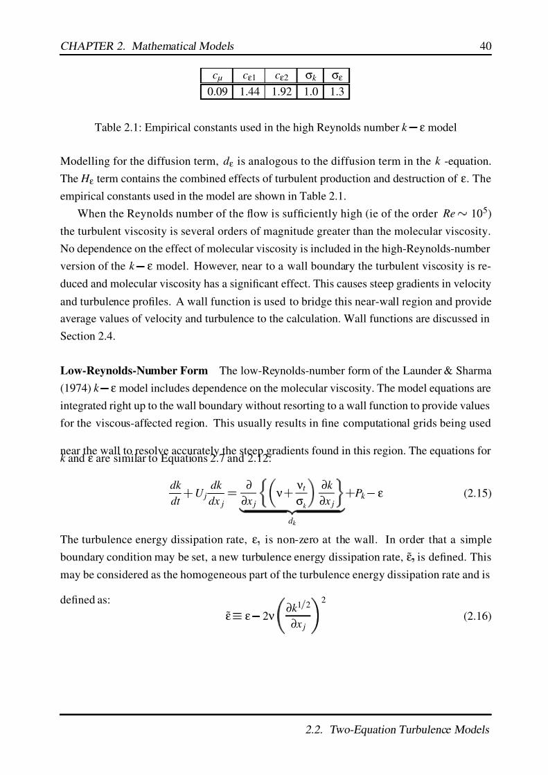
7/17/2019 Big
http://slidepdf.com/reader/full/big563db8d5550346aa9a975e13 59/189
CHAPTER 2. Mathematical Models 40
c µ cε1 cε2 σk σε
0.09 1.44 1.92 1.0 1.3
Table 2.1: Empirical constants used in the high Reynolds number k ε model
Modelling for the diffusion term, d ε is analogous to the diffusion term in the k -equation.
The H ε term contains the combined effects of turbulent production and destruction of ε. The
empirical constants used in the model are shown in Table 2.1.
When the Reynolds number of the flow is sufficiently high (ie of the order Re
105)
the turbulent viscosity is several orders of magnitude greater than the molecular viscosity.
No dependence on the effect of molecular viscosity is included in the high-Reynolds-number
version of the k ε model. However, near to a wall boundary the turbulent viscosity is re-
duced and molecular viscosity has a significant effect. This causes steep gradients in velocity
and turbulence profiles. A wall function is used to bridge this near-wall region and provide
average values of velocity and turbulence to the calculation. Wall functions are discussed in
Section 2.4.
Low-Reynolds-Number Form The low-Reynolds-number form of the Launder & Sharma
(1974) k ε model includes dependence on the molecular viscosity. The model equations are
integrated right up to the wall boundary without resorting to a wall function to provide values
for the viscous-affected region. This usually results in fine computational grids being used
near the wall to resolve accurately the steep gradients found in this region. The equations fork and ε are similar to Equations 2.7 and 2.12:
dk
dt U j
dk
dx j
∂
∂ x j
ν
νt
σk
∂k
∂ x j
d k
Pk
ε (2.15)
The turbulence energy dissipation rate, ε is non-zero at the wall. In order that a simple
boundary condition may be set, a new turbulence energy dissipation rate, ε is defined. This
may be considered as the homogeneous part of the turbulence energy dissipation rate and is
defined as:
ε ε 2 ν
∂k 1 2
∂ x j
2
(2.16)
2.2. Two-Equation Turbulence Models
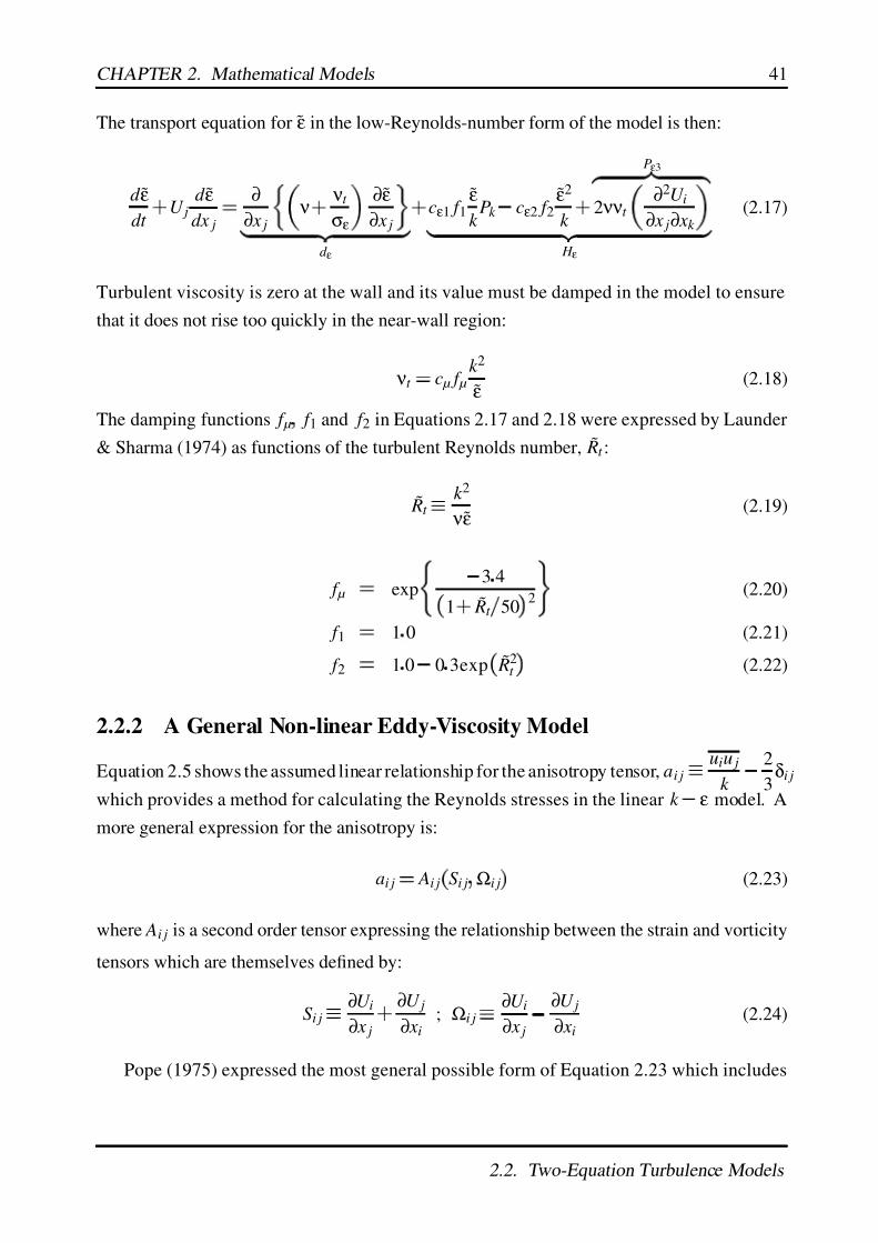
7/17/2019 Big
http://slidepdf.com/reader/full/big563db8d5550346aa9a975e13 60/189
CHAPTER 2. Mathematical Models 41
The transport equation for ε in the low-Reynolds-number form of the model is then:
d ε
dt
U jd ε
dx j
∂
∂ x j
ν
νt
σε
∂ε
∂ x j
d ε
cε1 f 1ε
k Pk
cε2 f 2ε2
k
Pε3
2 ννt
∂2U i
∂ x j∂ xk
H ε
(2.17)
Turbulent viscosity is zero at the wall and its value must be damped in the model to ensure
that it does not rise too quickly in the near-wall region:
νt c µ f µ
k 2
ε (2.18)
The damping functions f µ
f 1 and f 2 in Equations 2.17 and 2.18 were expressed by Launder
& Sharma (1974) as functions of the turbulent Reynolds number, ˜ Rt :
˜ Rt
k 2
νε (2.19)
f µ exp
3 4
1
˜ Rt
50
2
(2.20)
f 1 1
0 (2.21)
f 2 1
0 0
3exp
˜ R2t
(2.22)
2.2.2 A General Non-linear Eddy-Viscosity Model
Equation 2.5 shows the assumed linear relationship for the anisotropy tensor, ai j
uiu j
k
2
3δi j
which provides a method for calculating the Reynolds stresses in the linear k ε model. A
more general expression for the anisotropy is:
ai j
Ai j
S i j Ωi j
(2.23)
where Ai j is a second order tensor expressing the relationship between the strain and vorticity
tensors which are themselves defined by:
S i j
∂U i
∂ x j
∂U j
∂ xi; Ωi j
∂U i
∂ x j
∂U j
∂ xi(2.24)
Pope (1975) expressed the most general possible form of Equation 2.23 which includes
2.2. Two-Equation Turbulence Models

7/17/2019 Big
http://slidepdf.com/reader/full/big563db8d5550346aa9a975e13 61/189
CHAPTER 2. Mathematical Models 42
up to quintic products of the strain and vorticity tensors and can be written:
ai j
10
∑n
1
G
n T
n
i j (2.25)
T
1
i j
S i j
T
2
i j
S ik Ωk j Ωik S k j
T
3
i j
S ik S k j
1
3S lk S kl δi j
T
4
i j Ωik Ωk j
1
3Ωlk Ωkl δi j
T
5
i j Ωil S lmS m j S il S lmΩm j
T
6
i j Ωil ΩlmS m j S ilΩlmΩm j
2
3S lmΩmnΩnlδi j
T
7
i j Ωik S kl ΩlmΩm j Ωik Ωkl S lmΩm j
T
8
i j S ik Ωkl S lmS m j
S ik S kl Ωlm S m j
T 9
i j Ωik ΩklS lm S m j S ik S kl ΩlmΩm j 2
3S kl S lm ΩmnΩnk δi j
T
10
i j Ωik S kl S lmΩmnΩn j Ωik Ωkl S lmS mnΩn j
(2.26)
Setting the coefficients G
1
k
εc µ, G
n
0 for n 1, returns the linear stress-strain re-
lationship used in the Launder-Sharma k ε model (Equation 2.5). If the coefficients are
defined for G
n
1
a non-linear turbulence model is produced. Pope (2000) states that for
every algebraic stress model (and consequently, every differential stress model 1) there is a
corresponding non-linear eddy-viscosity model. The coefficients G
n can be derived from
the “parent” DSM and the cubic non-linear models of Apsley & Leschziner (1998) and Wallin
& Johansson (2000) use this approach. Taulbee (1992) and Gatski & Speziale (1993) have
proposed quintic models in which all ten G
n coefficients are non-zero.
2.2.3 Cubic Non-Linear k ε Model
High-Reynolds-Number Form The cubic non-linear expression for anisotropy developed
by Craft et al (1996b) is:
ai j
uiu j
k
2
3δi j (2.27)
The terms with coefficients c1
c2
c3
c4 and c5 correspond to the T
3
i j , T
2
i j , T
4
i j , T
5
i j and
T
6
i j terms in Equation 2.26 respectively. The c6 and c7 terms are both developed from the
T
1
i j term. Craft et al defined the coefficients for Equation ?? by “tuning” the model to a
number of reference flows:
1See Section 2.3 for a discussion of DSMs
2.2. Two-Equation Turbulence Models

7/17/2019 Big
http://slidepdf.com/reader/full/big563db8d5550346aa9a975e13 62/189
CHAPTER 2. Mathematical Models 43
c1 c2 c3 c4 c5 c6 c7
0.1 0.1 0.26 -10c2 µ 0 5c2 µ 5c2 µ
Table 2.2: Constants used in the non-linear EVM
Homogeneous shear flow: As ∂U
∂ y is the only velocity gradient the only non-zero com-
ponents of ai j are a11 a22
a33 and a12. This gives the condition that c5 c6
c7 0 and
c2 and
c1
c3 were optimized with the values 0.1 and 0.26 respectively by comparison to
experimental and DNS data.
Fully developed swirling shear flow: This is a fully developed pipe flow in which the
pipe rotates about its own axis. The U V and W velocities are defined in the axial ( x), radial
(r ) and circumferential (ψ ) directions. Although experiments show a non-linear increase of
circumferential mean velocity with radius (Cheah et al, 1993), any linear EVM (where vw
νt S 23 and S 23
∂W
∂r
W
r ) gives a linear variation of circumferential (swirl) velocity
with radius. No quadratic term appears in the nonlinear expression of vw, and consequently
a quadratic non-linear model will not improve the calculation of swirl velocity.
Flow with streamline curvature: In a fully developed curved channel flow, the curvature
leads to increased mixing near the concave wall and reduced mixing at the convex wall (Ellis
& Joubert, 1974). This leads to an asymmetric velocity profile across the channel. The
normal stresses do not affect the mean streamwise velocity or turbulence profiles but the
shear stress (uv) does. Furthermore, the expression for uv from Equation ?? contains linear
and cubic correlations of S i j
and Ωi j
, but no quadratic terms. As with the fully developed
swirling shear flow, this demonstrates that the non-linear model must be extended to at least
cubic level to improve the calculation of flow with streamline curvature.
The coefficients which Craft et al defined from the reference cases are shown in Table
2.2. The c5 coefficient is set to zero as no simple test case could be found to distinguish its
effect. (It acts in a similar manner to the c4 term in swirling flow and the c7 term in curved
channel flow.)
Craft et al also defined a modelled form of c µ, based on the strain and vorticity invariants:
c µ
0 3
1 0
35
max
S Ω
1 5
1
exp
0 36exp 0 75 max
S Ω
(2.28)
where the dimensionless strain and vorticity invariants are defined:
S
k
ε
S i jS i j
2; Ω
k
ε
Ωi jΩi j
2(2.29)
2.2. Two-Equation Turbulence Models
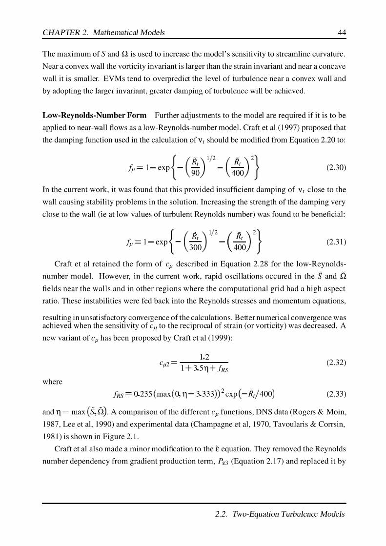
7/17/2019 Big
http://slidepdf.com/reader/full/big563db8d5550346aa9a975e13 63/189
CHAPTER 2. Mathematical Models 44
The maximum of S and Ω is used to increase the model’s sensitivity to streamline curvature.
Near a convex wall the vorticity invariant is larger than the strain invariant and near a concave
wall it is smaller. EVMs tend to overpredict the level of turbulence near a convex wall and
by adopting the larger invariant, greater damping of turbulence will be achieved.
Low-Reynolds-Number Form Further adjustments to the model are required if it is to be
applied to near-wall flows as a low-Reynolds-number model. Craft et al (1997) proposed that
the damping function used in the calculation of νt should be modified from Equation 2.20 to:
f µ 1 exp
˜ Rt
90
1 2
˜ Rt
400
2
(2.30)
In the current work, it was found that this provided insufficient damping of νt close to the
wall causing stability problems in the solution. Increasing the strength of the damping very
close to the wall (ie at low values of turbulent Reynolds number) was found to be beneficial:
f µ 1 exp
˜ Rt
300
1 2
˜ Rt
400
2
(2.31)
Craft et al retained the form of c µ described in Equation 2.28 for the low-Reynolds-
number model. However, in the current work, rapid oscillations occured in the S and Ω
fields near the walls and in other regions where the computational grid had a high aspect
ratio. These instabilities were fed back into the Reynolds stresses and momentum equations,
resulting in unsatisfactory convergence of the calculations. Better numerical convergence wasachieved when the sensitivity of c µ to the reciprocal of strain (or vorticity) was decreased. A
new variant of c µ has been proposed by Craft et al (1999):
c µ2
1 2
1 3 5η f RS
(2.32)
where
f RS 0 235
max
0 η 3 333
2exp
˜ Rt
400
(2.33)
and η max
S
Ω
. A comparison of the different c µ functions, DNS data (Rogers & Moin,
1987, Lee et al, 1990) and experimental data (Champagne et al, 1970, Tavoularis & Corrsin,
1981) is shown in Figure 2.1.
Craft et al also made a minor modification to the ε equation. They removed the Reynolds
number dependency from gradient production term, Pε3 (Equation 2.17) and replaced it by
2.2. Two-Equation Turbulence Models

7/17/2019 Big
http://slidepdf.com/reader/full/big563db8d5550346aa9a975e13 64/189
CHAPTER 2. Mathematical Models 45
1
S , to give:
Pε3 (2.34)
in which the effect is limited to the near wall region by ˜ Rto 250 and the empirical constant
is set as: cε3 0
0022.
2.2.4 Realizability Conditions
Schumann (1977) defined a set of realizability conditions for turbulence models. He high-
lighted that the Reynolds stresses must not exceed the limits set by the Schwarz inequality,
normal stress should not become negative nor should negative turbulent kinetic energy be
allowed during the calculation. Lumley (1978) considered that these were perhaps mathe-
matical niceties but recognized the importance of imposing the realizability conditions, sincea frequent cause of aborted calculations is the occurrence of negative energies. (These may
occur as a consequence of poor initial conditions or where one component of the Reynolds
stress is suppressed such as in stably stratified flow.)
Both Schumann (1977) and Lumley (1978) discuss the realizability conditions in the
context of a DSM. The realizability conditions may also be usefully applied in a linear EVM
in which the Reynolds stresses are determined by Equation 2.5. For example, in regions of
smooth flow, the values of k and ε will approach zero. Depending on how the lower limits
of k and ε are controlled in the calculation, this may result in large values of νt c µ
k 2
ε
.
If there is an inviscid deflection of the flow in this region, the velocity gradients will become
non-zero and when amplified by νt , may result in negative normal stresses. May (1998)
described a method of implementing the realizability conditions in an EVM which provides a
limiting maximum value for νt . This is described in Appendix A. It is not necessary to apply
the condition to the NLEVM of Craft et al (1996b) as when k 2
ε becomes very large, the
strain and vorticity invariants (S , Ω will also be large. As the NLEVM uses the functional
form of c µ (Equation 2.28) which contains the reciprocal of max
S Ω , c µ and consequently
νt will be reduced in regions of very high k 2
ε
2.3 Differential Stress Models
2.3.1 Basic DSM
In Section 2.2 it is shown how the Reynolds Averaged Navier-Stokes equations (Equation 2.3
& 2.4) can be closed by using an eddy-viscosity model to calculate the Reynolds stresses. A
2.3. Differential Stress Models

7/17/2019 Big
http://slidepdf.com/reader/full/big563db8d5550346aa9a975e13 65/189
CHAPTER 2. Mathematical Models 46
higher level of closure can be achieved if separate transport equations are calculated for the
individual Reynolds stresses: this is a differential stress model. The transport equations for
Reynolds stress include all the physical processes which act on the Reynolds stresses; they
are capable of accounting for history and non-local effects. This is not possible with an EVM
or NLEVM which rely on local velocity gradients to calculate the Reynolds stresses.Launder et al (1975) proposed a Reynolds stress transport equation:
Duiu j
Dt
uiuk
∂U j
∂ xk
u juk
∂U i
∂ xk
Pi j
φi j εi j
d i j
∂
∂ xk
ν∂uiu j
∂ xk
d νi j
(2.35)
The mean-flow convection Duiu j
Dt , production term Pi j and viscous diffusion term d νi j are
all in closed form and require no further modelling. The pressure-strain φ i j, dissipation εi j
and diffusion due to pressure-transport and turbulent convection d i j are:
φi j
p
ρ
∂ui
∂ x j
∂u j
∂ xi
(2.36)
εi j 2 ν∂ui
∂ xk
∂u j
∂ xk
(2.37)
d i j
∂
∂ xk
uiu juk
pui
ρ δ jk
pu j
ρ δik
(2.38)
All these terms require modelling. Local isotropy is assumed for the dissipative term:
εi j
2
3δi jε (2.39)
and a transport equation is solved for ε:
Dε
Dt
∂
∂ x j
cε
k
εuiu j
δi j ν
∂ε
∂ x j
1
2cε1
ε
k Pkk
cε2ε2
k (2.40)
The constants are: cε 0 18 cε1 1 44 and cε2 1 92. The generalized-gradient-diffusion
hypothesis of Daly and Harlow (1970) is adopted for the diffusion term (pressure-transport
and turbulent convection):
d i j
∂
∂ xk
csuk ul
k
ε
∂uiu j
∂ xl
(2.41)
with the coefficient cs 0
22.
The trace of the pressure-strain term (φii is zero and hence pressure-strain does not pro-
duce or destroy turbulence. Instead, it redistributes turbulent energy between the Reynolds
2.3. Differential Stress Models
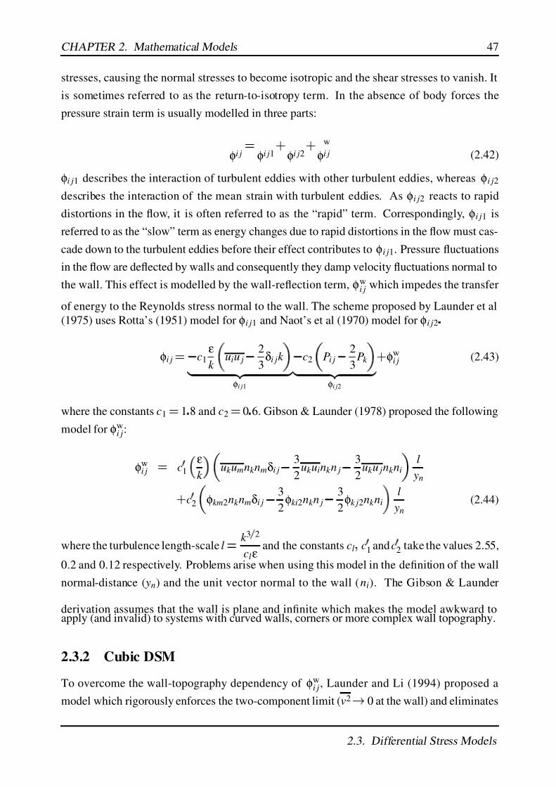
7/17/2019 Big
http://slidepdf.com/reader/full/big563db8d5550346aa9a975e13 66/189
CHAPTER 2. Mathematical Models 47
stresses, causing the normal stresses to become isotropic and the shear stresses to vanish. It
is sometimes referred to as the return-to-isotropy term. In the absence of body forces the
pressure strain term is usually modelled in three parts:
φi j
φi j1
φi j2
φ
w
i j (2.42)
φi j1 describes the interaction of turbulent eddies with other turbulent eddies, whereas φi j2
describes the interaction of the mean strain with turbulent eddies. As φi j2 reacts to rapid
distortions in the flow, it is often referred to as the “rapid” term. Correspondingly, φi j1 is
referred to as the “slow” term as energy changes due to rapid distortions in the flow must cas-
cade down to the turbulent eddies before their effect contributes to φi j1. Pressure fluctuations
in the flow are deflected by walls and consequently they damp velocity fluctuations normal to
the wall. This effect is modelled by the wall-reflection term, φwi j which impedes the transfer
of energy to the Reynolds stress normal to the wall. The scheme proposed by Launder et al
(1975) uses Rotta’s (1951) model for φi j1 and Naot’s et al (1970) model for φi j2
φi j
c1ε
k
uiu j
2
3δi jk
φi j1
c2
Pi j
2
3Pk
φi j2
φw
i j (2.43)
where the constants c1 1
8 and c2
0 6. Gibson & Launder (1978) proposed the following
model for φwi j:
φwi j
c
1
ε
k
uk umnk nmδi j
3
2uk uink n j
3
2uk u jnk ni
l
yn
c
2 φkm2nk nmδi j
3
2φki2nk n j
3
2φk j2nk ni
l
yn
(2.44)
where the turbulence length-scale l
k 3 2
cl ε and the constants cl
c
1and c
2 take the values 2.55,
0.2 and 0.12 respectively. Problems arise when using this model in the definition of the wall
normal-distance ( yn) and the unit vector normal to the wall ( ni). The Gibson & Launder
derivation assumes that the wall is plane and infinite which makes the model awkward toapply (and invalid) to systems with curved walls, corners or more complex wall topography.
2.3.2 Cubic DSM
To overcome the wall-topography dependency of φwi j, Launder and Li (1994) proposed a
model which rigorously enforces the two-component limit (v2
0 at the wall) and eliminates
2.3. Differential Stress Models

7/17/2019 Big
http://slidepdf.com/reader/full/big563db8d5550346aa9a975e13 67/189
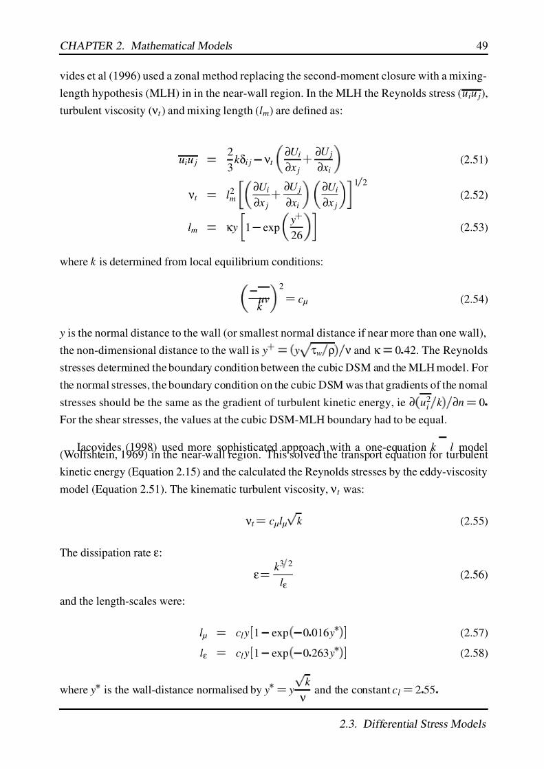
7/17/2019 Big
http://slidepdf.com/reader/full/big563db8d5550346aa9a975e13 68/189
CHAPTER 2. Mathematical Models 49
vides et al (1996) used a zonal method replacing the second-moment closure with a mixing-
length hypothesis (MLH) in in the near-wall region. In the MLH the Reynolds stress (uiu j),
turbulent viscosity ( νt ) and mixing length (lm) are defined as:
uiu j
2
3k δi j
νt
∂U i
∂ x j
∂U j
∂ xi
(2.51)
νt
l2m
∂U i
∂ x j
∂U j
∂ xi
∂U i
∂ x j
1 2
(2.52)
lm κ y 1 exp
y
26
(2.53)
where k is determined from local equilibrium conditions:
uvk
2
c µ (2.54)
y is the normal distance to the wall (or smallest normal distance if near more than one wall),
the non-dimensional distance to the wall is y
y τw
ρ
ν and κ 0
42. The Reynolds
stresses determined the boundary condition between the cubic DSM and the MLH model. For
the normal stresses, the boundary condition on the cubic DSM was that gradients of the nomal
stresses should be the same as the gradient of turbulent kinetic energy, ie ∂
u2i
k
∂n 0
For the shear stresses, the values at the cubic DSM-MLH boundary had to be equal.
Iacovides (1998) used more sophisticated approach with a one-equation k
l model(Wolfshtein, 1969) in the near-wall region. This solved the transport equation for turbulent
kinetic energy (Equation 2.15) and the calculated the Reynolds stresses by the eddy-viscosity
model (Equation 2.51). The kinematic turbulent viscosity, νt was:
νt c µl µ k (2.55)
The dissipation rate ε:
ε
k 3 2
lε(2.56)
and the length-scales were:
l µ
cl y
1 exp
0 016 y
(2.57)
lε cl y
1 exp
0 263 y
(2.58)
where y is the wall-distance normalised by y
y
k
ν and the constant cl
2 55
2.3. Differential Stress Models

7/17/2019 Big
http://slidepdf.com/reader/full/big563db8d5550346aa9a975e13 69/189
CHAPTER 2. Mathematical Models 50
2.4 Near-Wall Models
2.4.1 Introduction
In high-Reynolds-number flow remote from a wall, viscous stresses are small in compari-
son to the Reynolds (turbulent) stresses. As the wall is approached, the Reynolds stresses
diminish and viscous stresses become more influential and their effects must be included
in the momentum equations. Two approaches for this method have already been discussed:
low-Reynolds-number modelling in the context of a k ε model (Section 2.2.1) and zonal
modelling using either a mixing-length or k l model (Section 2.3.2). As these techniques
integrate the momentum equations right up to the wall, they require fine computational grids
in order to capture the steep velocity and turbulence profiles near the wall. This results in
additional computational expense and is often not practicable for large three-dimensional
calculations. An alternative method is to “bridge” the near-wall region with a wall function.The first computational cell spans the near-wall region and extends into the fully turbulent
flow. The wall shear-stress is used to account for the frictional force of the wall on the flow
and average values are calculated for production of turbulence and dissipation rate in the
near-wall cell.
The three wall functions which are used in the present study are described in this section.
These are the basic wall function used in the TEAM code (Huang et al, 1983) described in
Section 2.4.2 and the Chieng & Launder (1980) wall function used in the STREAM code
(Lien & Leschziner, 1994a)2 described in Section 2.4.3. The new Analytic Wall Function
(Gerasimov, 1999) which has been developed and implemented during this work is described
in Section 2.4.4.
2.4.2 Basic Wall Function
Log-Law of the Wall
At a wall the no slip condition is applied (U i 0 . Immediately adjacent to the wall ( y
5) is the viscous sublayer in which viscous stresses are significant and the velocity varies
linearly with the non-dimensional distance from the wall ( y
. Further away from the wall(30
y
300) there exists the inner turbulent region, and further still ( y
300) is the
outer turbulent region. The viscous sublayer and inner turbulent region blend in the buffer
layer (5
y
30). A schematic diagram of the near-wall velocity profile is shown in Figure
2.2.
2See Chapter 3 for detailed descriptions of the TEAM and STREAM codes.
2.4. Near-Wall Models

7/17/2019 Big
http://slidepdf.com/reader/full/big563db8d5550346aa9a975e13 70/189
CHAPTER 2. Mathematical Models 51
In the derivation of conventional wall functions such as Launder & Spalding (1972) and
Chieng & Launder (1980) a steady, two-dimensional boundary layer with zero pressure gra-
dient is assumed. The momentum equation for the boundary layer reduces to:
∂
∂ y
µ
∂U
∂ y
ρuv
0 (2.59)
In the inner turbulent region the viscous stresses are negligible and Equation 2.59 reduces to:
ρuv τw (2.60)
where the constant τw is the shear stress at the wall. Assuming local equilibrium (turbulence
is dissipated where it is produced) provides:
ρuv
ρl
2
m
∂U
∂ y
2
(2.61)
where the mixing length is proportional to the distance from the wall, lm κ y and the constant
is κ 0
42. Substitution of Equation 2.61 into Equation 2.60 yields the logarithmic velocity
profile for the inner turbulent region:
U
1
κ ln
Ey
(2.62)
where the non-dimensional wall-distance y
yU τ
ν
, the friction velocity U τ τw
ρ and
the integration constant E 9 793 for smooth walls. Due to the logarithmic velocity profile,
the inner turbulent region is sometimes referred to as the “log-law region”.
Wall Shear Stress, τw
When turbulence is in local equilibrium the ratio
uv
k is constant which provides the
definition of c µ :
c µ
uv
k
2
0 09 (2.63)
where the value 0 09 is suggested by measurements in the equilibrium regions of boundary
layer flows. The turbulent kinetic energy is assumed to be constant in the log-law region and
the value at the near-wall node (k p is taken in the basic wall function. The friction velocity
can be expressed in terms of k p:
k p
uv
c1
2
µ
U 2τ
c1
2
µ
(2.64)
2.4. Near-Wall Models
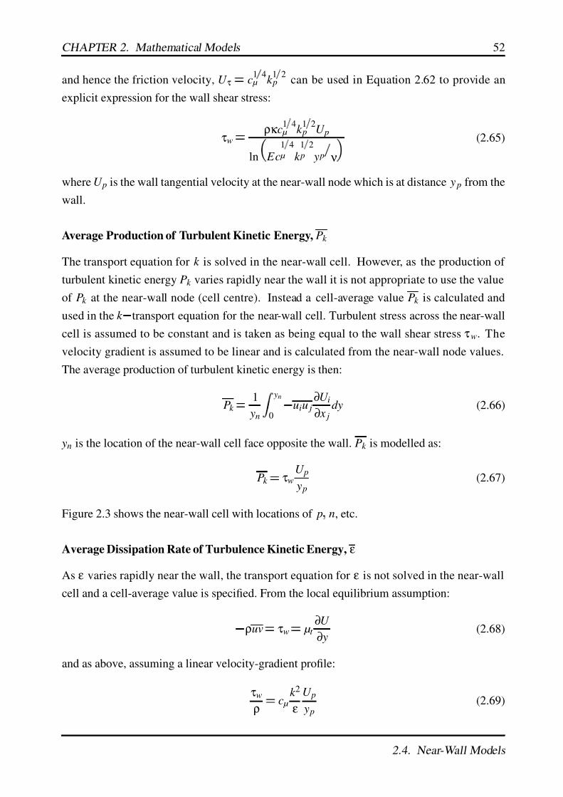
7/17/2019 Big
http://slidepdf.com/reader/full/big563db8d5550346aa9a975e13 71/189
CHAPTER 2. Mathematical Models 52
and hence the friction velocity, U τ c
1 4 µ k
1 2 p can be used in Equation 2.62 to provide an
explicit expression for the wall shear stress:
τw
ρκ c1 4
µ k 1 2 p U p
ln Ec1
4
µ k 1
2
p y p
ν
(2.65)
where U p is the wall tangential velocity at the near-wall node which is at distance y p from the
wall.
Average Production of Turbulent Kinetic Energy, Pk
The transport equation for k is solved in the near-wall cell. However, as the production of
turbulent kinetic energy Pk varies rapidly near the wall it is not appropriate to use the value
of Pk at the near-wall node (cell centre). Instead a cell-average value Pk is calculated and
used in the k transport equation for the near-wall cell. Turbulent stress across the near-wall
cell is assumed to be constant and is taken as being equal to the wall shear stress τ w. The
velocity gradient is assumed to be linear and is calculated from the near-wall node values.
The average production of turbulent kinetic energy is then:
Pk
1
yn
yn
0
uiu j∂U i
∂ x j
dy (2.66)
yn is the location of the near-wall cell face opposite the wall. Pk is modelled as:
Pk τw
U p
y p(2.67)
Figure 2.3 shows the near-wall cell with locations of p n, etc.
Average Dissipation Rate of Turbulence Kinetic Energy, ε
As ε varies rapidly near the wall, the transport equation for ε is not solved in the near-wall
cell and a cell-average value is specified. From the local equilibrium assumption:
ρuv τw
µt ∂U
∂ y(2.68)
and as above, assuming a linear velocity-gradient profile:
τw
ρ
c µ
k 2
ε
U p
y p(2.69)
2.4. Near-Wall Models
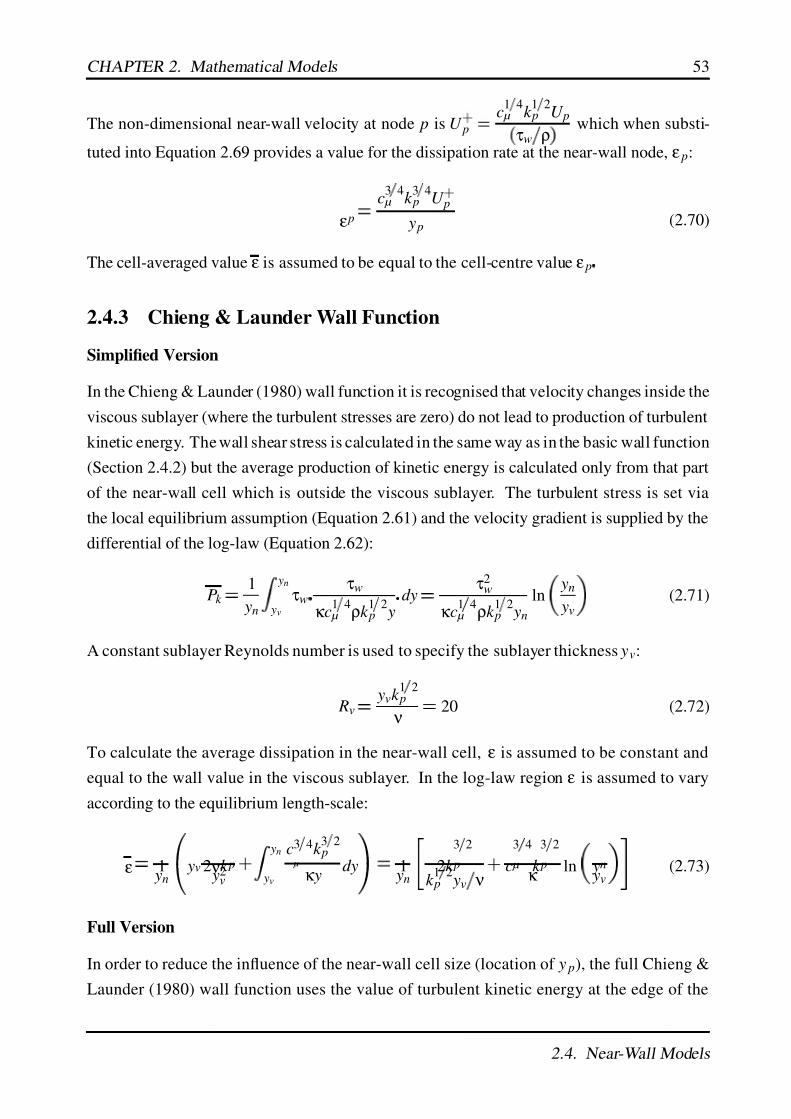
7/17/2019 Big
http://slidepdf.com/reader/full/big563db8d5550346aa9a975e13 72/189
CHAPTER 2. Mathematical Models 53
The non-dimensional near-wall velocity at node p is U p
c1 4
µ k 1 2 p U p
τw
ρ
which when substi-
tuted into Equation 2.69 provides a value for the dissipation rate at the near-wall node, ε p:
ε p
c3 4
µ k 3 4 p U
p
y p (2.70)
The cell-averaged value ε is assumed to be equal to the cell-centre value ε p
2.4.3 Chieng & Launder Wall Function
Simplified Version
In the Chieng & Launder (1980) wall function it is recognised that velocity changes inside the
viscous sublayer (where the turbulent stresses are zero) do not lead to production of turbulent
kinetic energy. The wall shear stress is calculated in the same way as in the basic wall function
(Section 2.4.2) but the average production of kinetic energy is calculated only from that part
of the near-wall cell which is outside the viscous sublayer. The turbulent stress is set via
the local equilibrium assumption (Equation 2.61) and the velocity gradient is supplied by the
differential of the log-law (Equation 2.62):
Pk
1
yn
yn
yv
τw
τw
κ c1 4
µ ρk 1 2 p y
dy
τ2w
κ c1 4
µ ρk 1 2 p yn
ln
yn
yv
(2.71)
A constant sublayer Reynolds number is used to specify the sublayer thickness yv:
Rv
yvk 1 2 p
ν
20 (2.72)
To calculate the average dissipation in the near-wall cell, ε is assumed to be constant and
equal to the wall value in the viscous sublayer. In the log-law region ε is assumed to vary
according to the equilibrium length-scale:
ε 1 yn
yv 2 νk p y2v
yn
yv
c3 4
µ
k 3 2 p
κ y dy 1
yn
2k
3 2
p
k 1
2
p yv
ν c
3 4
µ k
3 2
pκ
ln yn yv
(2.73)
Full Version
In order to reduce the influence of the near-wall cell size (location of y p), the full Chieng &
Launder (1980) wall function uses the value of turbulent kinetic energy at the edge of the
2.4. Near-Wall Models
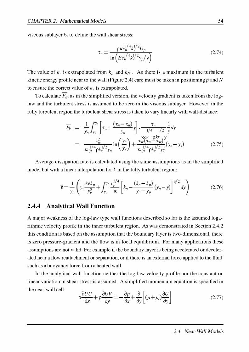
7/17/2019 Big
http://slidepdf.com/reader/full/big563db8d5550346aa9a975e13 73/189
CHAPTER 2. Mathematical Models 54
viscous sublayer k v to define the wall shear stress:
τw
ρκ c1 4
µ k 1 2v U p
ln
Ec1 4
µ k 1 2v y p
ν
(2.74)
The value of k v is extrapolated from k p and k N . As there is a maximum in the turbulent
kinetic energy profile near to the wall (Figure 2.4) care must be taken in positioning p and N
to ensure the correct value of k v is extrapolated.
To calculate Pk , as in the simplified version, the velocity gradient is taken from the log-
law and the turbulent stress is assumed to be zero in the viscous sublayer. However, in the
fully turbulent region the turbulent shear stress is taken to vary linearly with wall-distance:
Pk
1
yn
yn
yv
τw
τn τw
yn y
τw
κ c
1 4
µ ρk
1 2
v y
1
ydy
τ2w
κ c1
4
µ ρk 1
2
v yn
ln
yn
yv
τw
τn τw
κ c1
4
µ ρk 1
2
v y2n
yn yv
(2.75)
Average dissipation rate is calculated using the same assumptions as in the simplified
model but with a linear interpolation for k in the fully turbulent region:
ε
1
yn
yv
2 νk p
y2v
yn
yv
c3
4
µ
κ
k n
k n k p
yn y p
yn y
3 2
dy
(2.76)
2.4.4 Analytical Wall Function
A major weakness of the log-law type wall functions described so far is the assumed loga-
rithmic velocity profile in the inner turbulent region. As was demonstrated in Section 2.4.2
this condition is based on the assumption that the boundary layer is two-dimensional, there
is zero pressure-gradient and the flow is in local equilibrium. For many applications these
assumptions are not valid. For example if the boundary layer is being accelerated or deceler-
ated near a flow reattachment or separation, or if there is an external force applied to the fluid
such as a buoyancy force from a heated wall.
In the analytical wall function neither the log-law velocity profile nor the constant or
linear variation in shear stress is assumed. A simplified momentum equation is specified in
the near-wall cell:
ρ∂UU
∂ x
ρ∂UV
∂ y
∂ p
∂ x
∂
∂ y
µ µt
∂U
∂ y
(2.77)
2.4. Near-Wall Models
7/17/2019 Big
http://slidepdf.com/reader/full/big563db8d5550346aa9a975e13 74/189
CHAPTER 2. Mathematical Models 55
A prescribed viscosity profile is also adopted:
µt 0 for y yv
ρc µcl k 1
2
p
y yv for y
yv (2.78)
which is the Prandtl-Kolmogorov condition (Equation 1.8) and in which cl 2
55. The
simplified momentum equation is integrated to find analytical values of velocity gradient,
wall shear stress and average production of turbulent kinetic energy for the near-wall cell.
The derivation of these terms for an iso-thermal wall function is described in Appendix B
and they are summarised below. (The prime suffix denotes non-dimensional variables; the
subscript “re f ” denotes far-field reference values used to normalise the variables. The wall
function was derived in dimensionless terms for the version of STREAM in which it was
used.)
Wall Shear Stress:
τ w
k 1 2
p
ρre f
A1
Average Production of Turbulent Kinetic Energy:
Pk
ραk 1
2
p
yn
yn
yv
y
y v
A1
C 1 y v
C 2
y
yv
1 α
y
yv
2
dy
Constant Terms:
A1
αU n
C 2
yn
yv
C 1 y v
C 2α
ln
1 α
yn
yv
αC 1 y
2v
2
α yv
ln
1 α
yn
yv
C 1
ν
k p
∂ p
∂ x
γ U
∂U
∂ x
γ V
∂U
∂ y
C 2
ν
k p
∂ p
∂ x
U
∂U
∂ x
V
∂U
∂ y
Average Dissipation Rate:
ε
k 3 2
p
yn
2 ν
yε
1
clln
yn
yε
2.4. Near-Wall Models

7/17/2019 Big
http://slidepdf.com/reader/full/big563db8d5550346aa9a975e13 75/189
CHAPTER 2. Mathematical Models 56
γ is an empirical constant which is used to control the influence of convection inside the
laminar sub-layer, α
c µcl . The turbulence and dissipation viscous sublayer thicknesses yv
and yε are 10.8 and 5.1 respectively
2.4.5 Note on Near-Wall Distance
Two different methods are commonly used for the normalisation of the near-wall distance, y.
In the basic wall function (Section 2.4.2) the near-wall distance is normalised by the friction
velocity at the wall, U τ
τw
ρ, thus:
y
U τ y
ν (2.79)
In the derivation of the analytical wall function an alternative method is used, in which y is
normalised by using the turbulent kinetic energy at the near-wall node for the velocity scale:
y
k 1 2 p y
ν (2.80)
This method is used in the full Chieng & Launder wall function but with the turbulent kinetic
energy evaluated at the edge of the viscous sublayer (k v) rather than at the near-wall node
(k p). Equation 2.64 provides an alternative definition of U τ c
1 4
µ k 1
2
p , which allows y to be
re-cast in the same fashion as y :
y
c1
4
µ k 1
2
p y
ν (2.81)
Hence, y and y differ by a factor of c
1 4 µ
0 55
For a wall function to be applicable, the near-wall node must be placed outside the buffer
layer which blends the viscous sublayer and turbulent inner region, and within the upper limit
of the turbulent inner region (ie. the “log-law” region) shown in Figure 2.2. It is generally
held that the distance of the near-wall node from the wall should fall in the range 30
y
300. This equates to 55 y
550.
2.4. Near-Wall Models
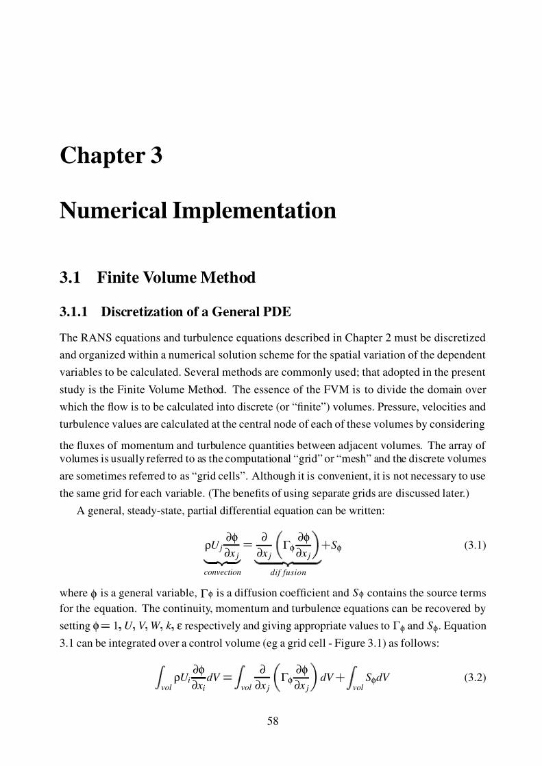
7/17/2019 Big
http://slidepdf.com/reader/full/big563db8d5550346aa9a975e13 76/189
Chapter 3
Numerical Implementation
3.1 Finite Volume Method
3.1.1 Discretization of a General PDE
The RANS equations and turbulence equations described in Chapter 2 must be discretized
and organized within a numerical solution scheme for the spatial variation of the dependent
variables to be calculated. Several methods are commonly used; that adopted in the present
study is the Finite Volume Method. The essence of the FVM is to divide the domain over
which the flow is to be calculated into discrete (or “finite”) volumes. Pressure, velocities and
turbulence values are calculated at the central node of each of these volumes by considering
the fluxes of momentum and turbulence quantities between adjacent volumes. The array of
volumes is usually referred to as the computational “grid” or “mesh” and the discrete volumes
are sometimes referred to as “grid cells”. Although it is convenient, it is not necessary to use
the same grid for each variable. (The benefits of using separate grids are discussed later.)
A general, steady-state, partial differential equation can be written:
ρU j∂φ
∂ x j
convection
∂
∂ x j Γ φ
∂φ
∂ x j
dif fusion
S φ (3.1)
where φ is a general variable, Γ φ is a diffusion coefficient and S φ contains the source terms
for the equation. The continuity, momentum and turbulence equations can be recovered by
setting φ 1 U
V
W
k
ε respectively and giving appropriate values to Γ φ and S φ. Equation
3.1 can be integrated over a control volume (eg a grid cell - Figure 3.1) as follows:
volρU i
∂φ
∂ xi
dV
vol
∂
∂ x j
Γ φ∂φ
∂ x j
dV
volS φdV (3.2)
58

7/17/2019 Big
http://slidepdf.com/reader/full/big563db8d5550346aa9a975e13 77/189
CHAPTER 3. Numerical Implementation 59
Then, by applying Gauss’ divergence theorem and grouping convection diffusion terms through
the same faces, one obtains:
area ρU φ Γ φ
∂φ
∂ x
dydz
e
w
area ρU φ Γ φ
∂φ∂ y
dxdz
n
s
area ρU φ Γ φ
∂φ
∂ z
dxdy
t
b
vol S φdV
(3.3)
Assuming that the variables are constant over each cell face, and defining the face areas as:
Ae w
dydz
e w; An
s
dxdz
n s; At
b
dxdy
t b then integration over the faces results in:
ρU φ A
e
ρU φ A
w
Γ φ A
∂φ
∂ x e
Γ φ A∂φ
∂ x w
ρV φ A
n
ρV φ A
s
Γ φ A ∂φ
∂ y n
Γ φ A ∂φ∂ y s
ρW φ A
t
ρW φ A
b
Γ φ A
∂φ
∂ z t
Γ φ A∂φ
∂ z b
vol S φdxdydz
(3.4)
The convection
ρU φ A
i diffusion Γ φ A∂φ
∂ x i
and source term need to be approxi-
mated for each grid cell in terms of the cell’s nodal value and the values at the surrounding
nodes. These terms are described initially for the one-dimensional computational cell (Figure
3.2) and then extended to three-dimensions.
Diffusion The diffusion term is calculated by the central difference scheme which assumes
that there is a linear variation in φ between adjacent nodes and constant gradient:
Γ φ∂φ
∂ x e
Γ φ
δ x e
φ E φP
(3.5)
(Note that in the one-dimensional system Ae w
1 and is not shown in Equation 3.5).
Convection It is well known that the central difference scheme is not generally suitable for
calculating the convection terms. It is not bounded1 and when the Peclet number2 Pe 2
oscillations in the value of φ between nodes can occur causing the solution to diverge. A
better treatment of convection is required.
1Scarborough (1958) proposed the following “boundedness” criteria for convection schemes (i) In the ab-
sence of sources, internal nodal values of φ should be bounded by the boundary values. (ii) All coefficients of
the discretized equations should have the same sign.2The Peclet number is the ratio expressing the relative magnitude of the convection across the grid cell to
the diffusion. Pe ρU ∆ x Γ where ∆ x is the grid-cell dimension.
3.1. Finite Volume Method
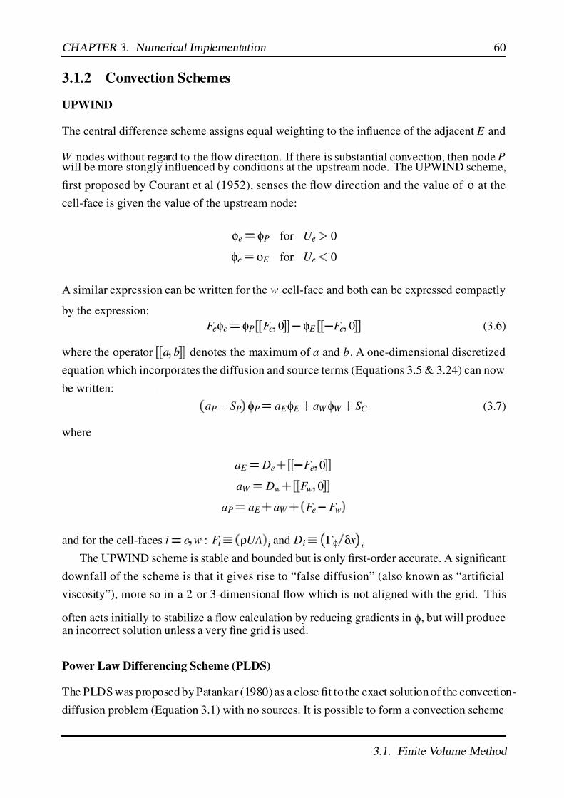
7/17/2019 Big
http://slidepdf.com/reader/full/big563db8d5550346aa9a975e13 78/189
CHAPTER 3. Numerical Implementation 60
3.1.2 Convection Schemes
UPWIND
The central difference scheme assigns equal weighting to the influence of the adjacent E and
W nodes without regard to the flow direction. If there is substantial convection, then node Pwill be more stongly influenced by conditions at the upstream node. The UPWIND scheme,
first proposed by Courant et al (1952), senses the flow direction and the value of φ at the
cell-face is given the value of the upstream node:
φe φP for U e
0
φe φ E for U e 0
A similar expression can be written for the w cell-face and both can be expressed compactly
by the expression:
F eφe φP
F e 0
φ E
F e 0 (3.6)
where the operator
a b denotes the maximum of a and b. A one-dimensional discretized
equation which incorporates the diffusion and source terms (Equations 3.5 & 3.24) can now
be written:
aP S P
φP a E φ E
aW φW S C (3.7)
where
a E
De
F e 0
aW
Dw
F w 0
aP a E
aW
F e F w
and for the cell-faces i
e
w : F i
ρUA
i and Di Γ φ
δ x i
The UPWIND scheme is stable and bounded but is only first-order accurate. A significant
downfall of the scheme is that it gives rise to “false diffusion” (also known as “artificial
viscosity”), more so in a 2 or 3-dimensional flow which is not aligned with the grid. This
often acts initially to stabilize a flow calculation by reducing gradients in φ, but will producean incorrect solution unless a very fine grid is used.
Power Law Differencing Scheme (PLDS)
The PLDS was proposed by Patankar (1980) as a close fit to the exact solution of the convection-
diffusion problem (Equation 3.1) with no sources. It is possible to form a convection scheme
3.1. Finite Volume Method

7/17/2019 Big
http://slidepdf.com/reader/full/big563db8d5550346aa9a975e13 79/189
CHAPTER 3. Numerical Implementation 61
from the exact solution (known as the “exponential convection scheme”) but it is expensive to
compute and is not exact for 2 and 3-dimensional problems or non-zero sources. The PLDS
is sensitive to the direction and relative strength of the flow expressed via the Peclet number:
Pee
10 ;
a E
De
Pee
10
Pee 0 ;
a E
De
1 0
1Pee
5 Pee
0 Pee 10 ;
a E
De
1 0 1Pee
5
Pee 10 ;
a E
De
0
which can be written:
a E
De
0
1
0 1 F e
5
De
0
F e
(3.8)
A similar expression can be defined for aW and these can be used to define a new version of
Equation 3.7. Like UPWIND, PLDS is first-order accurate but it is unconditionally bounded.
Quadratic Upstream Interpolation for Convection Kinetics (QUICK)
The QUICK scheme developed by Leonard (1979) uses a three point upstream-weighted
quadratic interpolation for the cell-face values, which fits through the two nodes either side
of the face and the next node upstream (Figure 3.3). The cell-face values are determined
from:
φe
3
8φ E
6
8φP
1
8φW for U e
0
φe
3
8φP
6
8φ E
1
8φ EE for U e 0
Thus the coefficients can be written:
a E De
3
8
F e 0
3
8F e (3.9)
aW
Dw
3
8
F w 0
3
8F w (3.10)
When using the QUICK scheme, the discretized PDE contains an additional source term
S Q which accounts for contributions from the nodes which are not directly adjacent to the
cell-face under consideration:
3.1. Finite Volume Method

7/17/2019 Big
http://slidepdf.com/reader/full/big563db8d5550346aa9a975e13 80/189
CHAPTER 3. Numerical Implementation 62
aP S P
φP
a E φ E
aW φW
S C
S Q (3.11)
where
S Q 18
F e 0
φW
F e 0
φ EE
F w 0
φWW
F w 0
φ E
1
8
F n 0 φS
F n 0 φ NN
F s 0 φSS
F s 0 φ N
1
8
F t 0 φ B
F t 0 φT T
F b 0 φ BB
F b 0 φT (3.12)
and
aP aW
a E
F e F w (3.13)
QUICK is third-order accurate with respect to its Taylor series truncation error and is
considerably more accurate than either UPWIND or PLDS. However, stability problems can
occur when using QUICK as it is not guaranteed to be bounded. This can lead to slight
under and over-shoots in the solution which can be a problem particularly when calculating
turbulent kinetic energy, dissipation or Reynolds normal stress (none of which can physically
be negative).
Upstream Monotonic Interpolation for Scalar Transport (UMIST)
From Equation 3.1 it is apparent that convection is represented by a first-order derivative
and its representation by a first-order scheme is sound on both physical and mathematical
grounds. However, unless calculated on very fine grids, first-order convection schemes do not
provide sufficient accuracy. As the interpolation polynomial on which all first-order schemes
are based is truncated at the second-order term, the second-order derivative provides the
largest error. Even-order derivatives are associated with the diffusion process, thus first-order
schemes tend to introduce “false diffusion”.
Improved accuracy can be obtained by using schemes having an order greater than two,
such as the QUICK scheme already described. However, such schemes introduce spurious
oscillations in the region of steep gradients of the transported variable when the Peclet number
is high. This is a problem for turbulence modelling in particular, as it can result in negative
values of the Reynolds stresses and turbulent dissipation. A method of overcoming these
oscillations is to add a component to the scheme which introduces, or strengthens, the bias
towards the upstream node. To ensure that monotonicity is preserved, the upstream biasing
must be controlled by the oscillatory features of the solution and this results in non-linear
schemes.
3.1. Finite Volume Method

7/17/2019 Big
http://slidepdf.com/reader/full/big563db8d5550346aa9a975e13 81/189
CHAPTER 3. Numerical Implementation 63
Harten (1983) proposed the Total Variation Diminishing (TVD) concept which was ex-
pressed for general conservation laws by Sweby (1984): Given a basic scheme which pre-
serves second-order accuracy in space and time, but which is unbounded, an appropriate
limiter is introduced which diminishes the oscillation-provoking, anti-diffusive truncation er-
ror on the basis of the TVD constraint. TVD schemes based on QUICK have been proposedby Leonard (1988) and Gaskell & Lau (1988). Both of these involve several condition state-
ments which lead to high computational expense. Lien & Leschziner (1994b) proposed a
continuous and highly compact QUICK-based scheme, the UMIST scheme, which is now
described.
For the iterative solution of statistically steady flows, the cell-face flux can be written:
φe φP
1
4
1 κ
φ E φP
1 κ
φP φW
(3.14)
where the values at the one-dimensional cell face (φe) and the surrounding nodes (φ E φP φW )
are defined in Figure 3.3 for flow in the direction west to east. Thus φe is given the upwind
value, φP, and an anti-diffusive component consisting of φ E φP and φW . The order of the
scheme can be set by κ . Setting κ 1
0and0
5 returns the central difference, UPWIND and
QUICK schemes respectively.
The variables are non-dimensionalised by φ
φ φW
φ E φP
and to make Equation 3.14 mono-
tonic, a slope limiter is introduced ϕ
r , in which:
r
φP
1 φP(3.15)
Equation 3.14 can now be expressed:
φe
φP
1
4
1 κ ϕ
r
1 κ r ϕ
1
r
1 φP
(3.16)
In order to ensure that symmetry is preserved - ie. that forward and backward gradients are
treated in the same manner - the following condition is imposed:
ϕ
r
r ϕ
1
r
(3.17)
and Equation 3.16 now becomes:
φe
φP
ϕ
r
2
1 φP
(3.18)
which is independent of κ . Sweby (1984) has shown that TVD arises from the constraint
ϕ
r
min
2r 2 for r
0 and ϕ
r
0 for r 0. Substituting the value for r from Equation
3.1. Finite Volume Method

7/17/2019 Big
http://slidepdf.com/reader/full/big563db8d5550346aa9a975e13 82/189
CHAPTER 3. Numerical Implementation 64
3.15 gives the following constraints for TVD:
φe 1
φe 2φP
φe
φP for 0
φP 1 (3.19)
φe
φP for φP 0 or φP 1
The limiter function proposed by Lien & Leschziner (1994b) for a symmetric, monotonic
form of QUICK is:
ϕ
r
max
0 min
2r 0
25
0
75r
0
75
0
25r
QUICK
2 (3.20)
which gives the following cell-face values:
φe
φP (3.21)
0
5max
0 min
2φP
1 φP
0
25
0 75φP
1 φP
0
75
0 25φP
1 φP
QUICK
2
1 φP
The matrix of equations for each variable is set up in the same fashion as the unbounded
QUICK scheme (Equation 3.11), only the additional source term is now given by:
S Q 0
5
F e 0 ϕ
r e
F e 0 ϕ
r e
φ E φP
F w 0
ϕ
r w
F w 0
ϕ
r w
φP
φW
F n 0 ϕ
r n
F n 0 ϕ
r n
φ N φP
F s 0 ϕ
r s
F s 0 ϕ
r s
φP φS
F t 0 ϕ
r t
F t 0 ϕ
r t
φT φP
F b 0 ϕ
r
b
F b 0 ϕ
r b
φP φ B
(3.22)
and
r e
φP φW
φ E φP
(3.23)
3.1.3 Source Term
The source term from Equation ?? is linearized as:
S φ
S C S Q
φPS P (3.24)
3.1. Finite Volume Method

7/17/2019 Big
http://slidepdf.com/reader/full/big563db8d5550346aa9a975e13 83/189
CHAPTER 3. Numerical Implementation 65
where S C usually contains constant contributions to the source term and S P the corresponding
sources which are a function of the dependent variable. To ensure stability of the solution it
is essential to maintain diagonal dominance in the matrices of discretized equations. As S P is
subtracted from the leading diagonal of the matrices, negative sources should be included in
S P, resulting in the addition of a positive value to the leading diagonal.
3.1.4 Three-Dimensional, Discretized, General PDE
Once all the coefficients have been specified according to the convection scheme, the full,
three-dimensional, general PDE can be written (cf. Equation 3.7):
aPφP ∑nb
anbφnb b (3.25)
a p ∑nb
anb S P∆ x∆ y∆ z
b
S C S Q
∆ x∆ y∆ z
where nb indicates the neighbouring nodes
E W
N
S
T
B and the coefficients anb are
specific to the convection scheme used. This defines the value of φ at a single node P; for
the whole grid, a matrix is assembled which is solved by a line-iterative method using a
Tri-Diagonal Matrix Algorithm (TDMA) with alternating sweep directions.
3.1.5 Calculation of Pressure
In the general PDE discussed so far (Equation 3.25) the pressure has not been stated explic-
itly but included in the source term. From the RANS equations there is no direct method of
specifing an equation for pressure. However, it is determined indirectly by way of the conti-
nuity equation: if the correct pressure field is used to determine the solution of the momentum
equations, then the continuity equation will be satisfied.
For a control volume in a staggered grid (Figure 3.4) the x-direction U -momentum equa-
tion for the node on face e can be written:
aeU e ∑nb
anbU nb
PP P E
Ae (3.26)
which is derived from the general PDE (Equation 3.25). The pressure force term which acts
on the control volume is
PP P E
Ae. A staggered grid is used with separate control volumes
for scalar quantities, U V and W (although only two dimensions representing U and V are
3.1. Finite Volume Method
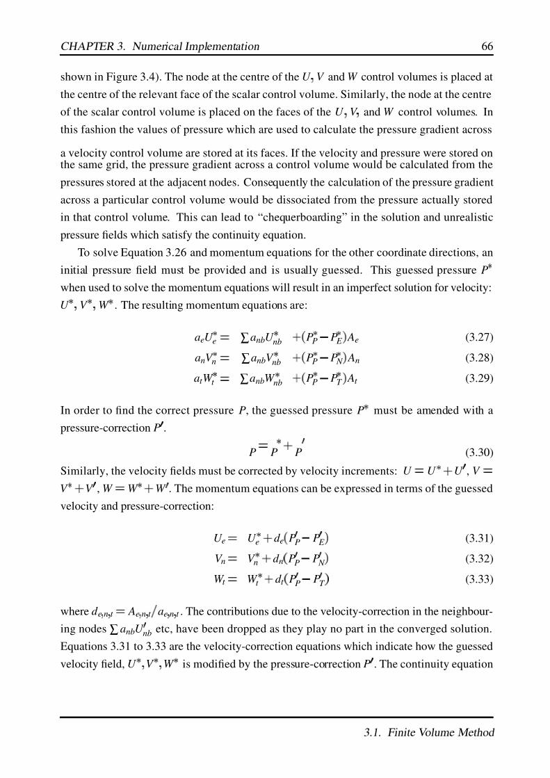
7/17/2019 Big
http://slidepdf.com/reader/full/big563db8d5550346aa9a975e13 84/189
CHAPTER 3. Numerical Implementation 66
shown in Figure 3.4). The node at the centre of the U V and W control volumes is placed at
the centre of the relevant face of the scalar control volume. Similarly, the node at the centre
of the scalar control volume is placed on the faces of the U
V and W control volumes. In
this fashion the values of pressure which are used to calculate the pressure gradient across
a velocity control volume are stored at its faces. If the velocity and pressure were stored onthe same grid, the pressure gradient across a control volume would be calculated from the
pressures stored at the adjacent nodes. Consequently the calculation of the pressure gradient
across a particular control volume would be dissociated from the pressure actually stored
in that control volume. This can lead to “chequerboarding” in the solution and unrealistic
pressure fields which satisfy the continuity equation.
To solve Equation 3.26 and momentum equations for the other coordinate directions, an
initial pressure field must be provided and is usually guessed. This guessed pressure P
when used to solve the momentum equations will result in an imperfect solution for velocity:
U
V
W . The resulting momentum equations are:
aeU e ∑ anbU nb
P P P E
Ae (3.27)
anV n ∑ anbV nb
P P P N
An (3.28)
at W t ∑ anbW nb
P P P T
At (3.29)
In order to find the correct pressure P, the guessed pressure P
must be amended with a
pressure-correction P .
P
P
P
(3.30)
Similarly, the velocity fields must be corrected by velocity increments: U U
U
, V
V
V , W W
W . The momentum equations can be expressed in terms of the guessed
velocity and pressure-correction:
U e
U e
d e
PP
P E
(3.31)
V n V
n d n
PP
P N
(3.32)
W t
W t
d t
PP
PT
(3.33)
where d e
n
t Ae
n
t
ae
n
t . The contributions due to the velocity-correction in the neighbour-
ing nodes ∑ anbU nb etc, have been dropped as they play no part in the converged solution.
Equations 3.31 to 3.33 are the velocity-correction equations which indicate how the guessed
velocity field, U
V
W is modified by the pressure-correction P
. The continuity equation
3.1. Finite Volume Method
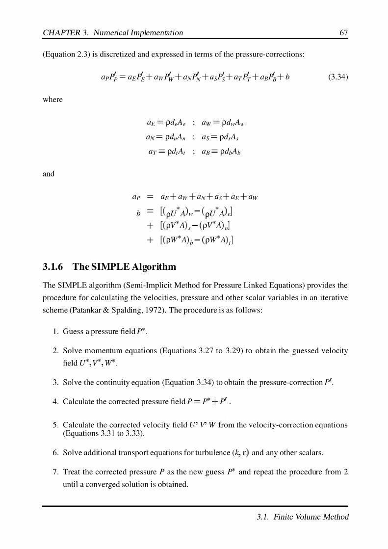
7/17/2019 Big
http://slidepdf.com/reader/full/big563db8d5550346aa9a975e13 85/189
CHAPTER 3. Numerical Implementation 67
(Equation 2.3) is discretized and expressed in terms of the pressure-corrections:
aPP P a E P E
aW P W a N P N
aS P S aT P T
a BP B b (3.34)
where
a E ρd e Ae ; aW
ρd w Aw
a N ρd n An ; aS ρd s As
aT ρd t At ; a B ρd b Ab
and
aP
a E
aW
a N
aS
a E
aW
b
ρU A
w
ρU A
e
ρV A
s
ρV A
n
ρW A
b
ρW A
t
3.1.6 The SIMPLE Algorithm
The SIMPLE algorithm (Semi-Implicit Method for Pressure Linked Equations) provides the
procedure for calculating the velocities, pressure and other scalar variables in an iterative
scheme (Patankar & Spalding, 1972). The procedure is as follows:
1. Guess a pressure field P .
2. Solve momentum equations (Equations 3.27 to 3.29) to obtain the guessed velocity
field U V
W
.
3. Solve the continuity equation (Equation 3.34) to obtain the pressure-correction P .
4. Calculate the corrected pressure field P
P
P .
5. Calculate the corrected velocity field U
V
W from the velocity-correction equations(Equations 3.31 to 3.33).
6. Solve additional transport equations for turbulence (k ε and any other scalars.
7. Treat the corrected pressure P as the new guess P and repeat the procedure from 2
until a converged solution is obtained.
3.1. Finite Volume Method
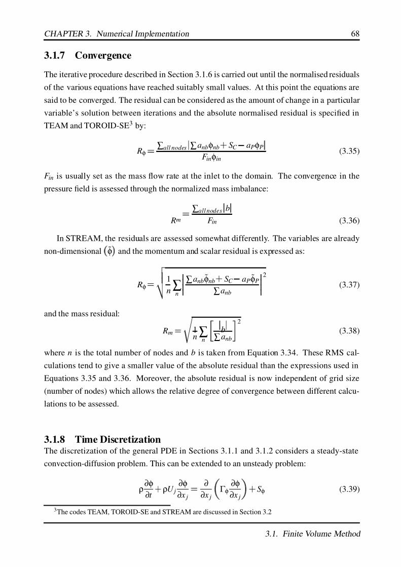
7/17/2019 Big
http://slidepdf.com/reader/full/big563db8d5550346aa9a975e13 86/189
CHAPTER 3. Numerical Implementation 68
3.1.7 Convergence
The iterative procedure described in Section 3.1.6 is carried out until the normalised residuals
of the various equations have reached suitably small values. At this point the equations are
said to be converged. The residual can be considered as the amount of change in a particular
variable’s solution between iterations and the absolute normalised residual is specified in
TEAM and TOROID-SE3 by:
Rφ
∑all nodes ∑ anbφnb S C
aPφP
F inφin(3.35)
F in is usually set as the mass flow rate at the inlet to the domain. The convergence in the
pressure field is assessed through the normalized mass imbalance:
Rm
∑all nodes b
F in (3.36)
In STREAM, the residuals are assessed somewhat differently. The variables are already
non-dimensional
φ
and the momentum and scalar residual is expressed as:
Rφ
1
n∑
n
∑ anbφnb S C
aPφP
∑ anb
2
(3.37)
and the mass residual:
Rm
1n ∑n
b∑ anb
2
(3.38)
where n is the total number of nodes and b is taken from Equation 3.34. These RMS cal-
culations tend to give a smaller value of the absolute residual than the expressions used in
Equations 3.35 and 3.36. Moreover, the absolute residual is now independent of grid size
(number of nodes) which allows the relative degree of convergence between different calcu-
lations to be assessed.
3.1.8 Time DiscretizationThe discretization of the general PDE in Sections 3.1.1 and 3.1.2 considers a steady-state
convection-diffusion problem. This can be extended to an unsteady problem:
ρ∂φ
∂t
ρU j∂φ
∂ x j
∂
∂ x j
Γ φ∂φ
∂ x j
S φ (3.39)
3The codes TEAM, TOROID-SE and STREAM are discussed in Section 3.2
3.1. Finite Volume Method

7/17/2019 Big
http://slidepdf.com/reader/full/big563db8d5550346aa9a975e13 87/189
CHAPTER 3. Numerical Implementation 69
For the purpose of derivation of the unsteady discretization, a simple one-dimensional diffu-
sion problem is studied. This will then be extended to the full convection-diffusion problem
and Equation 3.25 will be modified to a general PDE with fully implicit time-discretization.
The one-dimensional unsteady diffusion problem can be written:
ρ∂φ
∂t
∂
∂ x
Γ φ∂φ
∂ x
(3.40)
where Γ φ is the diffusion coefficient. Time can be considered as a grid coordinate which only
extends in one direction (Figure 3.5). The flow-field solution is calculated at time t and then
“marched” forward in time by a given timestep ∆t , and the flow-field is recalculated at time
t ∆t . Variables at the original time t are denoted by φ0
i and are known when calculating
variables at the new time t ∆t which are denoted by φ1
i . Integrating Equation 3.40 over the
control volume shown in Figure 3.5:
ρ
e
w
t
∆t
t
∂φ
∂t dtdx
t
∆t
t
e
w
∂
∂ x Γ φ
∂φ
∂ x
dxdt (3.41)
Assuming that the value φP is constant throughout a control volume at a given time and by
adopting the same discretization for diffusion as used in Section 3.1.1, then the unsteady
equation becomes:
ρ∆ x φ1
P φ0
P
t
∆t
t
Γ φ
δ x e
φ E φP
Γ φ
δ x w
φP φW
dt (3.42)
The profile of φ between φ0 and φ1 is assumed to take the general form:
t
∆t
t φPdt
θφ1
1 θ φ0 ∆t (3.43)
where θ is a weighting factor. Equation 3.42 can now be written:
ρ∆ x
∆t
φ1P
φ0P
θ
Γ φδ x
e
φ1 E
φ1P
Γ φδ x
w
φ1P
φ1W
(3.44)
1
θ
Γ φ
δ x e
φ0 E
φ0P
Γ φ
δ x w
φ0P
φ0W
On the understanding that variables at the old time
φ0
are known and that the variables at
the new time φ1
are unknown, the superscript “1” is dropped. The equation is rearranged
3.1. Finite Volume Method

7/17/2019 Big
http://slidepdf.com/reader/full/big563db8d5550346aa9a975e13 88/189
CHAPTER 3. Numerical Implementation 70
to give:
aPφP a E
θφ E
1 θ φ0 E
aW
θφW
1 θ φ0W
a0P
1 θ a E
1 θ aW φ0
P (3.45)
where
a E
Γ φ
δ x e
The value of θ which is chosen determines the nature of the time-discretization; three par-
ticular values, θ 0 0 5 and 1 give rise to the explicit, Crank-Nicholson and fully implicit
schemes respectively. In the explicit scheme, φP is not related to the values of φ E or φW at the
new time t ∆t and is expressed solely in terms of known variables at time t . A necessary
condition for accuracy in the explicit scheme is ∆t ρ
∆ x
2
2Γ φ. Hence when ∆ x is decreased to
improve spatial accuracy, ∆t must be decreased much more. The Crank-Nicholson scheme is
second-order accurate and unconditionally stable but requires ∆t
ρ
∆ x
2
Γ φto ensure bound-
edness. The fully implicit scheme is unconditionally stable for any size of time-step but re-
quires relatively small time-steps for accuracy. It has been recommended for time-dependent
calculations by Patankar (1980) and Versteeg & Malalasekera (1995) and all time-dependent
calculations carried out as part of the current work have used the fully implicit scheme.
The fully implicit scheme for a three-dimensional unsteady convection-diffusion problem
is (cf. Equation 3.25):
aPφP ∑nb
anbφnb b (3.46)
where
a p ∑anb a0 p
S P∆ x∆ y∆ z
a0 p ρ0
P
∆ x∆ y∆ z
∆t
b S C ∆ x∆ y∆ z
a0
Pφ0P
3.2 Codes Used
The standard UMIST codes have been adapted for the present research. Their capabilities
and structures are briefly summarized below.
3.2. Codes Used

7/17/2019 Big
http://slidepdf.com/reader/full/big563db8d5550346aa9a975e13 89/189
CHAPTER 3. Numerical Implementation 71
3.2.1 TEAM
TEAM (Turbulent Elliptic Algorithm - Manchester, Huang & Leschziner, 1983) is a two-
dimensional FVM code which uses a staggered grid system and SIMPLE pressure-correction
in two-dimensions. Time-dependent calculations are made with the fully implicit scheme
(Section 3.1.8). Several convection schemes are available: UPWIND, PLDS and QUICK.
In general, initial solutions for a steady-state problem are calculated with UPWIND. Time-
dependent calculations or final steady-state calculations are made with either QUICK on all
variables or with a combination of QUICK for the momentum equations and PLDS for the
turbulence equations. For calculations with the NLEVM, the shear stresses
uv are stored at
the scalar nodes (ie. they are not staggered as would be the normal practice in a DSM code).
This provides consistency between c µ and S Ω when calculating the functional form of c µ
(Equation 2.28) and is especially important in high aspect-ratio cells.
3.2.2 TOROID-SE
TOROID-SE calculates elliptic, turbulent flow and is principally intended for flow in curved
ducts. It is written in toroidal coordinates, which can be reduced to spherical, cylindrical
and Cartesian coordinates. The TEACH code on which it is based is very similar to TEAM
using a staggered grid with the SIMPLE algorithm for pressure-correction and including the
QUICK convection scheme. The code has both EVM and NLEVM turbulence models and
in a separate version a DSM. In the DSM version, shear stresses are stored at the corners
of the scalar cells, normal stresses at the scalar cell-centres. In the NLEVM version, all theReynolds stresses are stored at the scalar cell-centres as they are in the NLEVM version of
TEAM.
3.2.3 STREAM
Introduction
Simulation of Turbulent Reynolds-averaged Equations for All Mach numbers (Lien & Leschziner,
1994a), STREAM is a three-dimensional, fully elliptic, turbulent flow solver. It calcu-
lates flow using non-dimensional variables, on general non-orthogonal grids, using a non-
staggered (collocated) FVM. It uses the SIMPLE pressure-correction algorithm and has op-
tions for unsteady and compressible flow, and the UPWIND, QUICK and UMIST convection
schemes. STREAM is written in curvilinear coordinates in order to calculate the flow in non-
orthogonal grids. It uses the Rhie & Chow (1983) interpolation for pressure smoothing and
multi-block grids for efficient representation of complex geometries.
3.2. Codes Used
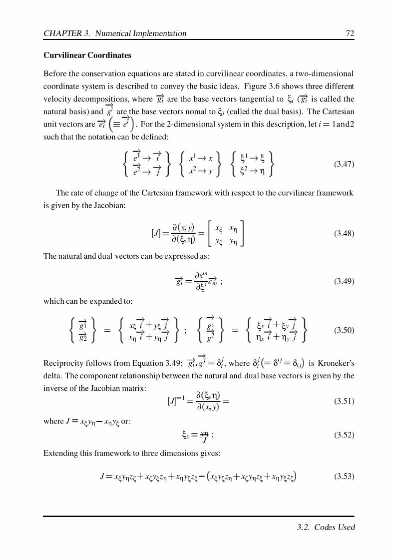
7/17/2019 Big
http://slidepdf.com/reader/full/big563db8d5550346aa9a975e13 90/189
CHAPTER 3. Numerical Implementation 72
Curvilinear Coordinates
Before the conservation equations are stated in curvilinear coordinates, a two-dimensional
coordinate system is described to convey the basic ideas. Figure 3.6 shows three different
velocity decompositions, where
gi are the base vectors tangential to ξi (
gi is called the
natural basis) and
gi are the base vectors nomal to ξi (called the dual basis). The Cartesian
unit vectors are
ei
ei
. For the 2-dimensional system in this description, let i 1and2
such that the notation can be defined:
e1
i
e2
j
x1
x
x2
y
ξ1
ξ
ξ2
η
(3.47)
The rate of change of the Cartesian framework with respect to the curvilinear framework
is given by the Jacobian:
J
∂
x y
∂
ξ η
xξ xη
yξ yη
(3.48)
The natural and dual vectors can be expressed as:
gi
∂ xm
∂ξi
em ; (3.49)
which can be expanded to:
g1
g2
xξ
i yξ
j
xη
i yη
j
;
g1
g2
ξ x
i ξ y
j
η x
i η y
j
(3.50)
Reciprocity follows from Equation 3.49:
gi
g j δ
ji , where δ
ji δi j
δi j
is Kroneker’s
delta. The component relationship between the natural and dual base vectors is given by the
inverse of the Jacobian matrix:
J
1
∂
ξ η
∂
x
y
(3.51)
where J xξ yη
xη yξ or:
ξ x
yη J
; (3.52)
Extending this framework to three dimensions gives:
J
xξ yη zζ
xζ yξ zη
xη yζ zξ
xξ yζ zη
xζ yη zξ
xη yξ zζ
(3.53)
3.2. Codes Used
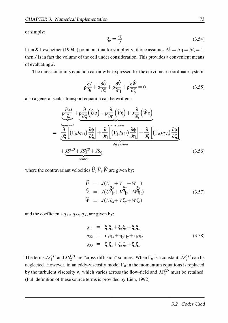
7/17/2019 Big
http://slidepdf.com/reader/full/big563db8d5550346aa9a975e13 91/189
CHAPTER 3. Numerical Implementation 73
or simply:
ξ x
zζ
J (3.54)
Lien & Leschziner (1994a) point out that for simplicity, if one assumes ∆ξ ∆η
∆ζ
1,
then J is in fact the volume of the cell under consideration. This provides a convenient means
of evaluating J .
The mass continuity equation can now be expressed for the curvilinear coordinate system:
ρ∂ J
∂t ρ
∂
U
∂ξ ρ
∂
V
∂η ρ
∂
W
∂ζ 0 (3.55)
also a general scalar-transport equation can be written :
ρ∂φ J
∂t
transient
ρ
∂
∂ξ
U φ
ρ
∂
∂η
V φ
ρ
∂
∂ζ
W φ
convection
∂
∂ξ Γ φ Jq11
∂φ
∂ξ
∂
∂η Γ φ Jq22
∂φ
∂η
∂
∂ζ Γ φ Jq33
∂φ
∂ζ
dif fusion
JS CD
1 JS CD
2 JS φ
source
(3.56)
where the contravariant velocities U
V
W are given by:
U
J
U ξ x
V ξ y
W ξ z
V
J
U η x
V η y
W η z (3.57)
W
J
U ζ x
V ζ y
W ζ z
and the coefficients q11
q22
q33 are given by:
q11 ξ xξ x ξ yξ y ξ zξ z
q22 η xη x η yη y η zη z (3.58)
q33 ζ xζ x ζ yζ y ζ zζ z
The terms JS CD1
and JS CD2
are “cross-diffusion” sources. When Γ φ is a constant, JS CD2
can be
neglected. However, in an eddy-viscosity model Γ φ in the momentum equations is replaced
by the turbulent viscosity νt which varies across the flow-field and JS CD2
must be retained.
(Full definition of these source terms is provided by Lien, 1992)
3.2. Codes Used

7/17/2019 Big
http://slidepdf.com/reader/full/big563db8d5550346aa9a975e13 92/189
CHAPTER 3. Numerical Implementation 74
Rhie-Chow Interpolation
It is often more convenient to collocate the flow variables at the same nodes in a non-staggered
grid. This is particularly true when using a non-orthogonal grid and it is the practice adopted
in STREAM. A problem with this practice is that the pressure gradient for a given cell must
be calculated from the adjacent cells. Thus the pressure gradient used in the momentum
equations for a given cell is dissociated from the actual value of pressure in that cell. This
can lead to “chequerboard” oscillations in which physically unrealistic pressure and velocity
fields will satisfy continuity. To prevent the pressure and velocity from becoming dissoci-
ated, Rhie & Chow (1983) proposed a scheme in which the pressure gradient used in the
momentum equations is corrected to capture pressure variations between adjacent nodes.
The non-staggered grid arrangement is shown in Figure 3.7. The equation can be written
for the one-dimensional situation is:
U P
∑nb anbU nb
aP
S C
H P
Pw Pe
J ∂ξ
∂ x
aP
DU P
(3.59)
which may also be written:
U P H P
DU P
Pw Pe
(3.60)
The Rhie & Chow interpolation for cell-face velocity is:
U e
1
2
U P
DU
P
Pw
Pe
P
U E
DU
E
Pw
Pe
E
1
2
DU P
DU E
PP P E
(3.61)
which may be written:
U e
1
2
U P
U E
linearinterpolation
(3.62)
1
2
DU
P
DU E
PP P E
DU P
Pw Pe
P DU
E
Pw Pe
E
pressuresmoothing
Equations 3.61 and 3.62 provide different ways of interpreting the Rhie & Chow interpola-
tion. In Equation 3.61 the velocity at the east face (U e) is directly linked to the two adjacent
pressure nodes
PP P E
. A different point of view is conveyed by Equation 3.62 which
states that the interpolation practice consists of a centred approximation for U e with an addi-
tional pressure smoothing term.
3.2. Codes Used

7/17/2019 Big
http://slidepdf.com/reader/full/big563db8d5550346aa9a975e13 93/189
CHAPTER 3. Numerical Implementation 75
Multi-Block Strategy
The multi-block strategy used in STREAM allows efficient grids to be generated for complex
geometries. The blocks are topological hexahedra and each block constitutes a self-contained
grid of cells. Adjacent blocks must match precisely along their common block-faces. Hence
all cells that lie on a block-face which adjoins another block, must align with a cell in the
adjacent block. “Hanging” nodes4are not permitted (Figure 3.8). Similarly, complete block-
faces must match complete block-faces - ie. it is not permitted to join a portion of a block-face
to an adjoining block-face, even if all the individual interfacing cells match precisely (Figure
3.9). “C” and “O” grids are permitted but have not been used in the present work.
Before calculation of the flow-field, STREAM extends each block by an additional two
nodes for each cell on a block-face which adjoins another block 5. The computational cells for
these additional nodes are referred to as “halo cells” and each halo cell is associated with the
relevant interior cell in the adjoining block. This association between halo cells and interiorcells of adjoining blocks is used to transfer flow-field and other calculation variables between
the blocks.
During the calculation of the flow-field, the variables stored at the halo cells are updated
by assigning the revelant value from the associated interior cell of the adjacent block. For
each iteration, the momentum equations are calculated for all the cells in the grid (this is Step
2 in the SIMPLE algorithm, Section 3.1.6). The halo cells are then updated with the values
of U V andW from the relevant interior nodes. After the pressure has been calculated and
the velocities corrected (Step 5 in the SIMPLE algorithm) the values of U
V
W and P in the
halo cells are updated.
4A “hanging” node is the term given to a boundary node on the face of block which does not share the
same spatial location as a node in an adjoining block. In this arrangement the grid lines do not match between
adjacent blocks.5Two cells are required for calculation of higher-order convection schemes such as QUICK.
3.2. Codes Used

7/17/2019 Big
http://slidepdf.com/reader/full/big563db8d5550346aa9a975e13 94/189
Chapter 4
Cylinder of Square Cross-Section Placed
Near a Wall
4.1 Introduction
Flow past a square cross-section cylinder is a popular test case and several groups have taken
measurements and made calculations of flow around the cylinder in a free-stream (as has been
discussed in Chapter 1). More recently, a number of researchers have taken measurements
and made calculations of the flow around square cylinders placed near to a wall. Notable
amongst these are the measurements of Durao et al (1991) and Bosch et al (1996) and the
calculations of Franke & Rodi (1993) and Bosch & Rodi (1996).
The popularity of this test case is due to the complex flow which is created by a rela-
tively simple geometry. The cylinder is a bluff body, there is stagnation of the flow at the
impingement point on the leading face and separation as the flow passes the leading edges.
Bending of the flow around the leading edges creates streamwise curvature and there is large-
scale separation and recirculation in the wake. Depending on how close the cylinder is to
the wall, the wake flow will either be steady or there will be periodic shedding of vortices
from the trailing edges. Durao et al and Bosch et al have shown that below a wall distance
of g
d 0 35 (Figure 1.1) the wake is steady and above g
d 0 50 there is regular vortex
shedding. Between these distances the wake fluctuates between steady and vortex sheddingbehaviour.
Although the flow past a square cylinder provides an essentially two-dimensional test
case, it mimics several features of flow around road vehicles: impingement, streamwise cur-
vature, separation and wake recirculation. The square cross-sectioned cylinder is thus an
appropriate test case for turbulence models which are intended for use in calculating the flow
around road vehicles.
77
7/17/2019 Big
http://slidepdf.com/reader/full/big563db8d5550346aa9a975e13 95/189
CHAPTER 4. Cylinder of Square Cross-Section Placed Near a Wall 78
The flow around the cylinder at three distances from the wall has been calculated: g
d
0 25
0
50 and 0
75. These three distances were chosen to cover the range of flow types: at
g
d 0
25 the wake is steady, at g
d 0
50 the cylinder is just far enough away from the
wall to generate periodic vortex shedding and at g
d 0 75 the periodic vortex shedding is
well established. These three distances coincide with the distances used in the measurementsby Durao et al (1991) and Bosch et al (1996). Durao et al measured the flow with g
d 0
25
and 0.50 at a Reynolds number Re 13 600; Bosch et al measured the flow with g
d 0 75
at a Reynolds number of Re 22 000.
In general there is no vortex shedding in the wake of a road vehicle, thus the calculation
with the steady wake, g
d 0
25, is the most relevant. Only this case is discussed in the
remainder of this Chapter; the discussion of the calculations of the remaining two cases is
included in Appendix C. When calculating the flow around the Ahmed body, a modified
form of the c µ function used in the non-linear k ε model was tested (Chapter 7). The flow
around the square cylinder has been recalculated for the case with g
d 0 25 using the non-
linear model with the modified c µ function to establish the effect of that modification on this
flow. The results of this calculation are discussed in Appendix D.
4.2 Models Used
Two turbulence models have been used to calculate the flow around the square cross-section
cylinder: the “standard” linear k ε model of Launder & Spalding (1974) and the non-linear
k
ε model of Craft et al (1996b) which are both described in Section 2.2. All calculations
have been made using the QUICK scheme to calculate convection of the mean velocities and
PLDS scheme for convection of turbulent kinetic energy and dissipation (Section 3.1.2). The
basic wall function described in Section 2.4.2 is used to “bridge” the viscosity-affected flow
in the near-wall regions around the cylinder and lower wall. All cases were calculated using
the implicit time-discretization scheme1 (Section 3.1.8). As this scheme is only first-order
accurate, a relatively small time-step was used to ensure accuracy, ∆t =0.009 to 0.014. This
corresponded to there being between 50 and 100 time-steps per vortex shedding cycle for
the cases g
d 0
50 and 0
75. All calculations were made using the TEAM code (Section
3.2.1).
1Durao et al and Bosch et al have both shown that with a wall-distance of g d
0
25 the wake is steady
and there is no vortex shedding. However, this case was calculated as a time-dependent flow to ensure that the
steady wake was calculated and not imposed by the solver.
4.2. Models Used
7/17/2019 Big
http://slidepdf.com/reader/full/big563db8d5550346aa9a975e13 96/189
CHAPTER 4. Cylinder of Square Cross-Section Placed Near a Wall 79
4.3 Domain, Grids, Boundary Conditions
4.3.1 Domain and Grid
The general domain used for calculation of all three cases is shown in Figure 1.1. It extended
from 10d upstream of the leading face of the cylinder to 20d downstream (d is the diameter
of the cylinder). The lower wall extended 6d in front of the cylinder in accordance with the
measurements of Bosch et al (1996) and the height of the domain was 10 d . A sample of the
grid used for the case g
d 0 25 is shown in Figure 4.1 (showing every second grid line only
for clarity). The grids used with each value of g
d had 102x72 cells which was comparable
to that used by Bosch & Rodi (1996) which had 106x75 cells. To establish that a grid-
independent solution could be obtained with this number of cells, preliminary calculations
were carried out using the linear k ε model for the case with g
d 0 25 and using the
102x72 cell grid and a refined grid with 132x96 cells. No significant differences were foundbetween the mean velocities, turbulent kinetic energy or dissipation calculated on the two
grids. All further calculations were made with the 102x72 cell grid.
4.3.2 Boundary Conditions
Inlet boundary conditions were set for each case according to the relevant set of measure-
ments. The cases with g
d 0
25 and 0.50 were to be compared with the measurements of
Durao et al (1991) and used an inlet Reynolds number Re 13
600 (based on d ) and inlet
turbulence intensity of 6%. The case with g
d
0
75 was to be compared with the mea-surements of Bosch et al (1996) and used an inlet Reynolds number of Re
22 000 and 4%
turbulence intensity. Neither Durao et al nor Bosch et al provide sufficient information to be
able to specify an inlet value for turbulence energy dissipation rate. Following the method
used by Bosch & Rodi (1996) for their calculations, the inlet dissipation rate was specified
for all three cases by assuming νt
ν 10 at the inlet. To test the sensitivity of the models to
this value, a second set of calculations for g
d 0
25 were carried out assuming νt
ν 100
at the inlet (following the method used by Franke & Rodi, 1991).
All values at the inlet were specified with uniform profiles. A zero-gradient condition was
imposed on all variables at the downstream boundary and symmetry planes were specified on
the upper domain boundary and the initial 4d of the lower domain boundary (ie. the portion
of the lower boundary which was upstream of the wall).
4.3. Domain, Grids, Boundary Conditions

7/17/2019 Big
http://slidepdf.com/reader/full/big563db8d5550346aa9a975e13 97/189
CHAPTER 4. Cylinder of Square Cross-Section Placed Near a Wall 80
4.4 Calculated Flow Results for g d 0 25
All calculated and measured results are normalised by the inlet streamwise velocity U o. The
measured data of Durao et al (1991) were not available in digital form and were therefore
re-digitized from the journal paper with a consequent loss in accuracy.
4.4.1 High Dissipation Inlet Condition ( νt
ν 10)
Drag and Lift
Coefficients of drag (C D) and lift (C L) are shown in Figure 4.2. The large oscillations in both
coefficients for time t 35 are due to the formation of starting vortices (all calculations were
started from a zero velocity inital flow-field). These are convected downstream and do not
influence the flow around the cylinder after t
45.
C D and C L calculated by the linear k ε model settle to constant values, indicating that the
calculated flow is steady: C D 1
77 and C L
0 28. However, there are small oscillations in
both C D and C L calculated by the non-linear k ε model throughout the period of calculation.
The mean value of C D calculated by the non-linear model is the same as that calculated by
the linear model (C D 1
77) but the mean value of C L is somewhat lower (C L
0 46).
Although Durao et al did not present detailed results for lift and drag, they did present power
spectra of vv for different distances of the cylinder from the wall. Durao et al use these to
show that there is no dominant frequency in the flow when g
d 0
5 and hence no vortex
shedding. However, in the power spectrum for g
d
0
25, there is a small peak whichoccurs at a non-dimensional frequency, f
f
d
U o
0 51. The frequency of the oscillations
in C D and C L calculated by the non-linear k ε model is f
0 40. The reasons why the
linear model does not calculate this oscillation are presented with the discussion of calculated
Reynolds stresses below2.
Velocity Profiles
Profiles of instantaneous U and V -velocity are shown in Figures 4.3 and 4.4 respectively.
Both models calculate the separation of the flow above the cylinder but the non-linear k
εmodel calculates a taller region of separated flow, with weaker reverse flow than the linear
model. Also, the non-linear model calculates a steeper velocity gradient than the linear model
in the upper shear layer above the cylinder and in the wake. In general, the non-linear model
2It is noted that the similarity in f between the measurements and non-linear calculation in itself does not
prove that the oscillations are due to the same effect. However, it provides some confidence that the non-linear
k ε model has calculated the flow accurately.
4.4. Calculated Flow Results for g
d 0 25
7/17/2019 Big
http://slidepdf.com/reader/full/big563db8d5550346aa9a975e13 98/189
CHAPTER 4. Cylinder of Square Cross-Section Placed Near a Wall 81
does not calculate the downstream wake as accurately as the linear model. The length of the
recirculating-flow region behind the cylinder, calculated by either model, is too long.
The steep velocity gradients and long recirculating flow regions calculated by the non-
linear k ε model have been shown for similar cases by Suga et al (2000) and Craft et al
(1999). Suga et al calculated the flow over a surface mounted cube using the low-Reynolds-number k ε A2 form of the non-linear model (Suga, 1995) in which A2 is the second
invariant of the anisotropic stress tensor3. They found that the calculated reattachment length
behind the cube was nearly twice as long as that measured. Also the downstream velocity
profile calculated by the k ε A2 model was rather worse than that calculated by a linear
k ε model.
Craft et al (1999) used the low-Reynolds-number form of the non-linear k ε model
(Section 2.2.3) to calculate the flow in an abrupt pipe expansion. The pipe expansion had
a step height 60% of that of the radius of the larger (downstream) pipe. Craft et al found
that the non-linear and linear k ε models calculated the same reattachment length but that
this was somewhat longer than the measured length. Comparison of the velocity profiles in
Figure 4.3 with the work of Suga et al and Craft et al provides confidence that the non-linear
model has calculated the flow correctly, to within the limitation of the model.
Reynolds Stress Contours
Durao et al (1991) present contour plots of three Reynolds stresses ( uu vv
uv) around the
cylinder. These are reproduced in Figures 4.5 to 4.7 with plots showing the Reynolds stresses
calculated by the linear and non-linear k ε models (all three figures use the same contour
values). The uu-stress calculated by both models (Figure 4.5) is in general too low. The
measured uu-stress has a normalised, peak value of 0.125 in the upper shear layer at x
d
4 0. The non-linear model calculates the magnitude of the peak uu-stress more accurately
than the linear model but this is too far downstream at x
d
7 0. The same trends for the
calculated vv and uv stresses are shown in Figures 4.6 and 4.7.
In the Figure 4.2 it was noted that whereas the linear k ε model calculated steady values
of C D and C L, a small oscillation was calculated by the non-linear model. In Figure 4.5, it
can be seen that the linear model calculates much higher levels of Reynolds stress aroundthe cylinder, particularly in the shear layer immediately above the cylinder. The linear model
calculates the Reynolds stresses from the product of turbulent viscosity and velocity gradients
(Equation 2.5). Above the cylinder, the linear model calculates less steep velocity gradients
than the non-linear model (Figure 4.3) and yet it calculates higher values of Reynolds stress.
3A transport equation is solved for A2 with the principal effect of improving the near-wall flow which in the
current work is bridged by the wall function.
4.4. Calculated Flow Results for g
d 0 25
7/17/2019 Big
http://slidepdf.com/reader/full/big563db8d5550346aa9a975e13 99/189
CHAPTER 4. Cylinder of Square Cross-Section Placed Near a Wall 82
This implies that the turbulent viscosity calculated by the linear k ε model is higher than
that calculated by the non-linear model. It is this increased level of νt which suppresses the
small oscillations in C D and C L calculated by the linear k ε model.
The increased level of νt is itself due to the high level of turbulent kinetic energy which
the linear k
ε model calculates around the cylinder. The linear model calculates too muchPk at the flow impingement; the subsequent high level of turbulent kinetic energy is convected
around the cylinder. In contrast, the non-linear k ε model reduces c µ in regions of high S
and Ω (Equation 2.28) and has a more sophisticated stress-strain relationship (Equation 2.27).
In calculating the impinging flow at the front of the cylinder, it does not produce the too high
levels of Pk and k which are calculated by the linear model. Due to the relatively large amount
of dissipation which has been assumed at the inlet for this calculation, relatively low levels
of turbulent kinetic energy are calculated in the flow which impinges on the cylinder. Hence,
the relatively high levels of turbulent kinetic energy calculated by the linear k ε model at
impingement do not show particularly well on Figures 4.5 to 4.7. The effect is much more
evident in the calculations with νt
ν 100 (Section 4.4.2).
Durao et al (1991) used an LDV technique to measure the flow. This was not able to
distinguish between “stresses” due to turbulent fluctuations (ie. Reynolds stresses u iu j) and
“stresses” due to any small oscillations in the shear layers or other periodic motions in the
flow. The periodic velocity can be defined by:
ui
U i ui
(4.1)
where U i is the instananeous velocity and ui
is the ensemble average. Thus time average
“stress” due to periodic motion measured by Durao et al is ui ui. If there was indeed a small
oscillation in the shear layers measured by Durao et al, then the values shown by them as
“Reynolds stresses” are in fact the time average total stresses:
ut iut
j uiu j
ui u j (4.2)
This could account for the higher levels of “Reynolds stress” which are measured, in com-
parison to the calculated levels.
4.4.2 Low Dissipation Inlet Condition ( νt
ν 100)
Drag and Lift
C D and C L for the case with a low rate of turbulence energy dissipation specificied at the
inlet are shown in Figure 4.8. After the starting effects have diminished both the linear and
4.4. Calculated Flow Results for g
d 0 25
7/17/2019 Big
http://slidepdf.com/reader/full/big563db8d5550346aa9a975e13 100/189
CHAPTER 4. Cylinder of Square Cross-Section Placed Near a Wall 83
non-liner k ε models calculate steady values for C D and C L. The low dissipation rate causes
higher levels of turbulent kinetic energy to remain in the flow as it reaches the cylinder.
This leads to higher levels of turbulent viscosity which are sufficient to suppress the small
oscillations in the shear layers and wake which were previously calculated by the non-linear
k
ε model.The non-linear k ε model calculates C D
1 81 and C L
0 48, which are close to
the mean values calculated with the high level of inlet dissipation. Similarly, the linear k ε
model calculates C D 1 86 but there is a marked difference in lift: C L 0 05 (cf. C L
0 28
for high dissipation case).
Velocity Profiles
Figure 4.9 shows the U -velocity profiles calculated by the two models with the low inlet dis-
sipation rate. The U -velocity calculated by the non-linear k
ε model is virtually unchangedin comparison to the high inlet dissipation rate calculation (Figure 4.3). However, the pro-
files calculated by the linear model are in still closer agreement with the measured values,
particularly in the downstream wake.
Reynolds Stress Contours
Reynolds stress contours (uu) are shown for the two models in Figure 4.10; differences are
apparent in the values calculated by both models compared to the high inlet dissipation case
(Figure 4.5). The non-linear k
ε model calculates a higher level of uu-stress in the shearlayer immediately above the cylinder. The location of the peak value in the upper shear layer
is calculated closer to the cylinder ( x
d 5
5) and closer to the location of the measured peak
value ( x
d 4
0). It is the increased level of Reynolds stress (and hence turbulent viscosity)
in the shear layer above the cylinder which is responsible for the suppression of periodic
oscillations in this region.
The high levels of uu-stress calculated by the linear k ε model on the leading face
of the cylinder demonstrate the process which was described in Section 4.4.1. The linear
model calculates too-high levels of Pk at impingement, leading to high levels of turbulent
kinetic energy which are convected around the cylinder, producing the high levels of uu
stress in Figure 4.10. The non-linear k ε model calculates production of kinetic energy at
impingement more accurately due to the functional form of c µ (Equation 2.28) and the non-
linear stress-strain relationship (Equation 2.27). The Reynolds stresses calculated in the shear
layers by the non-linear model are primarily due to the velocity gradients present rather than
high levels of turbulent kinetic energy convected from upstream. The linear k ε model was
4.4. Calculated Flow Results for g
d 0 25

7/17/2019 Big
http://slidepdf.com/reader/full/big563db8d5550346aa9a975e13 101/189
CHAPTER 4. Cylinder of Square Cross-Section Placed Near a Wall 84
developed by reference to simple shear flows and where the flow more closely matches this
situation (eg. in the wake) the excessive levels of Reynolds stress soon dissipate.
4.5 Conclusions
The comparison of the calculated results is compromised somewhat by not knowing the inlet
dissipation rate which was used in either Durao’s et al or Bosch’s et al experiments. The linear
k ε model calculates the mean velocity profiles more accurately than the non-linear model.
Also, the accuracy of the mean velocity profiles calculated by the linear model improves
when the lower dissipation rate inlet condition is used, whereas there is very little difference
in the profiles calculated by the non-linear model when considering either inlet condition. In
contrast, the Reynolds stresses calculated by the linear k ε model are considerably worse
than those calculated by the non-linear model and worsen when the lower dissipation rateinlet condition is used.
There is no experimental data available for the drag and lift generated on a square cylinder
placed near a wall and it is not possible to determine whether the linear or non-linear k ε
model has performed better in this respect. However, the coefficients of drag and lift are of
use in demonstrating differences between the models. When the high dissipation rate inlet
condition is used, the non-linear k ε model calculates a minor oscillation in drag and lift.
There is some justification for this oscillation presented by Durao et al (1991). When the low
dissipation rate inlet condition is used, this oscillation is attenuated by the higher levels of
turbulent viscosity, but the mean values of C D and C L are approximately the same for both
cases calculated by the non-linear model. There is a large change in C L calculated by the
linear model with the different inlet conditions and its sign changes from negative to positive
when the inlet dissipation rate is reduced.
The non-linear k ε model calculates Reynolds stresses more accurately than the linear
model. As the inlet boundary is sufficiently far upstream in this test case, the calculation of
the flow around the cylinder by the non-linear model is not greatly affected by alterations
in the turbulence boundary condtition. With its less accurate stress-strain model, the linear
k ε model is very sensitive to the upstream turbulence boundary condition. In industrial
calculations, full details of the upstream inlet condition are not usually known and must
instead be estimated. In such instances, it is far more desirable that the turbulence model
used is insensitive to minor changes in the upstream boundary condition if the flow is likewise
insensitive.
Calculations of the flow with g
d 0 50 and 0 75 are presented in Appendix C. With the
cylinder at these distances from the wall, vortices are shed periodically in the wake. Both the
4.5. Conclusions

7/17/2019 Big
http://slidepdf.com/reader/full/big563db8d5550346aa9a975e13 102/189
CHAPTER 4. Cylinder of Square Cross-Section Placed Near a Wall 85
linear and non-linear k ε models are capable of calculating this vortex-shedding behaviour.
When considering the calculation of time-averaged mean velocities, both models calculate the
flow with greater accuracy than the flow with g
d 0
25 and a steady wake. The frequency
of vortex shedding is calculated more accurately by the non-linear model.
The non-linear k
ε model calculates time-averaged total stresses more accurately thanthe linear model. However, the calculated distribution of the total stress between the “pe-
riodic” and Reynolds stresses is the opposite to that measured. The calculated total stress
consists of a large “periodic stress” and small Reynolds stress; the measured total stress con-
sists of a small “periodic stress” and large Reynolds stress.
4.5. Conclusions
7/17/2019 Big
http://slidepdf.com/reader/full/big563db8d5550346aa9a975e13 103/189
Chapter 5
Flow in a U-bend of Square Cross-Section
5.1 Introduction
The flow in a U-bend of square cross-section provides a searching test case for turbulence
models. Through the U-bend the flow is subjected to significant straining, and the radial
pressure gradient which is present induces secondary motion across the streamwise direction.
This secondary motion is further modified by anisotropies in the Reynolds stresses which are
generated at the corners of the duct. Indeed, these Reynolds stress anisotropies are known to
induce secondary motion even in a straight duct. The streamwise curvature of the U-bend and
streamwise vorticity generated are both present in road vehicle external flows, particularly
around the front edges of the vehicle and in its wake.
In this Chapter, calculated results are presented for the flow in a square cross-section U-
bend with strong curvature. The Reynolds number of the flow is Re 58
000 based on the
streamwise bulk velocity, W b and hydraulic diameter, D; the radius of curvature of the bend
is Rc
D 3
35. With this radius of curvature, the flow does not separate from the inner wall
of the U-bend. This is the test case for which Chang et al (1983a) and Choi et al (1990) have
carried out measurements and for which calculations have been made by several groups (see
discussion in Chapter 1).
5.2 Models Used
Two turbulence models have been used to calculate the flow in the U-bend: the non-linear
k ε model of Craft at al (1996b) and the cubic DSM of Craft et al (1996a). The linear k ε
model has not been used for this case as the flow is very sensitive to the Reynolds stress
anisotropies. Calculations by Chang et al (1983a,b), Johnson & Launder (1985), Azzola et al
86

7/17/2019 Big
http://slidepdf.com/reader/full/big563db8d5550346aa9a975e13 104/189
CHAPTER 5. Flow in a U-bend of Square Cross-Section 87
(1986) and Choi et al (1989) have all shown the ineffectiveness of the linear k ε model in
calculating this flow (Section 1.3.2). The current calculations with the non-linear k ε model
are compared instead to calculations with the cubic DSM1.
Although the final method for calculating the flow around the Ahmed body (Chapter 7)
will use wall functions, they have not been used for this test case. Chang et al (1983a,b)showed that a linear k ε model with wall functions is particularly poor at calculating this
flow. Azzola et al (1986) showed that a low-Reynolds-number model using the MLH in the
fine near-wall cells improved the calculation of flow in a circular cross-section duct. Also,
Choi et al (1989) showed that near-wall pressure variations are significant at the corners
of the duct; these cannot be calculated by the coarse near-wall cell employed by the wall
functions described in Section 2.4. The calculations presented in this Chapter should hence
be considered as a test of the non-linear k ε model in isolation and not the combined non-
linear model and wall function method.
The flow has been calculated with low-Reynolds-number models using a zonal approach.
A one-equation k l model was used to calculate the near-wall flow and either the non-linear
k ε model (Craft et al, 1996b) or cubic DSM (Craft et al, 1996a) was used to calculate
the core flow. (This is slightly different from the approach used by Iacovides et al (1996)
which used the cubic DSM with a MLH model in the near-wall zone.) In the near-wall zone,
the one-equation model uses the eddy viscosity hypothesis (Equation 2.5) with the turbulent
viscosity, νt , provided by:
νt
c µ
k
lm (5.1)
and the mixing length, lm:
lm 2 4Y 1 exp
y
Am
(5.2)
where Y is the smallest normal distance to the wall, y
Y
k
ν, and Am is a damping
function set according to the particular solution strategy adopted. Preliminary calculations
showed that if the original form of the near-wall turbulence damping in the one-equation
model was retained (Equation 5.2; Am 62 5 as used by Iacovides et al., 1996), then a con-
stant c µ 0 09 had to be used in the k l model across the near-wall zone to give the correct
wall profile of the streamwise velocity. This model is hereinafter refered to as NLEVM-1.
When the functional form of c µ (Equation 2.28) was used in the near-wall zone, it was found
that the damping function in Equation 5.2 had to be reduced to Am 31
25 to retain the cor-
1The cubic DSM is the most advanced turbulence model used with the steady RANS equations, currently
employed at UMIST.
5.2. Models Used
7/17/2019 Big
http://slidepdf.com/reader/full/big563db8d5550346aa9a975e13 105/189
CHAPTER 5. Flow in a U-bend of Square Cross-Section 88
rect near-wall profile of streamwise velocity (Figure 5.1). This model is hereinafter refered
to as NLEVM-2. Calculated results are presented for both NLEVM-1 and NLEVM-2.
In the cubic DSM calculation, the Reynolds stress transport equations were solved across
the core region only. The k -transport equation was solved in the near-wall region to provide
values of turbulent kinetic energy for the one-equation model.All calculations were made using the TOROID-SE code (Section 3.2.2) and the QUICK
convection scheme (Section 3.1.2).
5.3 Domain, Grids, Boundary Conditions
5.3.1 Domain and Grid
A sketch of the U-bend used for the flow measurements by Chang et al (1983a) and Choi et
al (1990) is shown in Figure 1.2. The z-coordinate is in the streamwise direction. Negative
values of z are used to indicate the distance in the entry section upstream of the start of the
curved section; positive values of z indicate distance from the end of the curved section in the
downstream tangent. Angular distance around the curved section is denoted by α.
A second sketch of the calculated domain in Figure 5.2 shows the lengths of the upstream
and downstream tangents (6 125 D and 12
9 D respectively, where D is the hydraulic diam-
eter of the duct). Only half the duct was calculated, with a symmetry plane placed at the
mid-height of the duct ( y 0). The grid used for all calculations had 67 x 35 nodes in the
cross-stream planes (Figure 5.3). 87 planes were used in the streamwise direction of which:25 were used in the upstream tangent, 42 in the U-bend itself and the remaining 20 in the
downstream tanget (Figure 5.4). This grid has been tested previously and calculations on it
using the cubic DSM found to be grid independent (Iacovides, 1999). The only modification
to the grid previously tested was to extend the grid in the tangent downstream of the bend.
The original grid used a constant inter-plane distance in the streamwise direction. The modi-
fication adopted in this study was to apply a geometric expansion of 1.1 to successive planes
downstream of the bend. In this way the downstream tangent was extended, whilst main-
taining the same number of streamwise planes. The one-equation k l model was applied
over the first twelve nodes adjacent to the wall in the cross-stream plane. The zone interface
between the one-equation model and the NLEVM or DSM in the core flow was at y
100.
5.3.2 Upstream Boundary Condition
To define the fully-developed, upstream inlet boundary condition, a pre-calculation in a
straight duct was carried out for each model. The straight duct used cyclic boundary condi-
5.3. Domain, Grids, Boundary Conditions
7/17/2019 Big
http://slidepdf.com/reader/full/big563db8d5550346aa9a975e13 106/189
CHAPTER 5. Flow in a U-bend of Square Cross-Section 89
tions for mean velocities and turbulence variables at its inlet and outlet. The fully developed
profiles resulting from this pre-calculation were prescribed at the inlet to the upstream tangent
of the U-bend.
5.4 Calculated Flow Results
All calculated and measured results are normalised by the bulk streamwise velocity W b.
5.4.1 Comparison to Calculated Data
Two comprehensive data sets for the square U-bend experiment are readily available in the
literature: Chang et al (1983a) and Choi et al (1990). Different experimental methods were
used, with LDA being adopted by Chang et al and hot-wire anemometry being adopted by
Choi et al. Discrepancies between these sets of data are descibed in Section 1.3.2. In the
following discussion, calculated results are compared to Choi’s et al data. This is not because
Choi’s et al results are thought to be more accurate, rather that these results are available in
electronic form on the ERCOFTAC database. (The results of Chang et al would have had
to be re-digitised from a journal with subsequent loss of accuracy.) The exception is where
values are compared upstream of the U-bend ( z
D
1). Here Choi et al did not take any
measurements and calculated values are compared to Chang’s et al data.
5.4.2 Inlet Flow Profiles
Inlet profiles of the streamwise velocity (W ), secondary velocities (U
V ) and cross-stream
normal stresses (uu, vv) are shown in Figure 5.5 for the NLEVM-2 and cubic DSM calcu-
lations. These are the fully developed flow profiles on the duct centreline ( y 0) from the
pre-calculations in the straight duct with cyclic boundary conditions. The NLEVM-2 model
calculates a small difference between uu and vv and the weak secondary flow which is in-
duced can be seen in the U -velocity directing flow from the walls to the centre of the duct.
The cubic DSM calculates a much larger difference in the normal stresses which in turn
induces a larger secondary velocity in the inlet profile.
5.4.3 Velocity Profiles
The streamwise (W
W b) and cross-stream (U
W b) velocity profiles are shown in Figures
5.6 and 5.7. There is very close agreement between both sets of NLEVM calculation and
5.4. Calculated Flow Results
7/17/2019 Big
http://slidepdf.com/reader/full/big563db8d5550346aa9a975e13 107/189
CHAPTER 5. Flow in a U-bend of Square Cross-Section 90
the cubic DSM. Where there are differences between the NLEVM-1 and NLEVM-2, the
calculations using NLEVM-2 are in general slightly closer to the DSM results.
The “hole” in the W -velocity profile which appears between α 90o
135o is calculated
reasonably well, except on the centreline where the peak and trough near the inside wall is
not calculated. In Section 1.3.2 the differences between the measured data of Chang et al andChoi et al are discussed and the W -velocity profiles are compared in Figure 1.5. Chang et
al measured a much lower level of W -velocity on the centreline at α 130o than Choi et al
did at α 135o; the calculated W -velocity from all three models is in closer agreement with
Chang’s et al data than with Choi’s et al at this location.
Also shown in Figure 5.6 is the W -velocity calculated by Choi et al (1989) using a linear
k ε model with a MLH model in the near-wall region. (This is shown for two positions
around the bend: α 90o and 135o. It should be noted that the results shown at α
135o were
actually calculated at α 130o by Choi et al.) The W -velocity calculated by the NLEVMs is
in much closer agreement with that calculated by the cubic DSM than is the linear k ε /MLH
calculation of Choi et al. Also the NLEVMs and cubic DSM calculate the W -velocity more
accurately than the linear k ε /MLH in comparison to the measured data. This is particularly
notable at the centreline (2 y
D 0) but differences between the models lessen towards the
top wall (2 y
D 1 0).
The cross-stream U -velocity is calculated in reasonable agreement with the results of
Choi et al results up to α 90o
At the half-way point in the bend, the measured results
suggest that there is a positive U -velocity (fluid flowing from the inside to the outside of the
bend) from the centreline (2 y
D
0) to near the top wall of the duct (2 y
D
0
75). However,the calculated results show that the negative return flow is already present at 2 y
D 0
75
This would imply that in the measured flow, the return flow path must be confined to a small
region very close to the top wall of the duct and by continuity this must be relatively fast
moving fluid. In contrast, the calculations predict a much deeper region of return flow, with
consequently lower velocity. By the end of the bend (α 180o) the measurements show that
there is still a strong secondary motion across the duct, whereas the calculations predict a
much weaker overall secondary motion.
5.4.4 Reynolds Stress Profiles
Profiles of the Reynolds stresses are shown for the three normal stresses (uu, vv, ww) and
one shear stress (uw) in Figures 5.8 to 5.11 respectively. Differences between the Reynolds
stresses calculated by the NLEVM models and cubic DSM are more significant than the
differences in the mean velocities discussed in Section 5.4.3. As the cubic DSM solves a
separate transport equation for each of the Reynolds stresses (Equation 2.35), it incorporates
5.4. Calculated Flow Results

7/17/2019 Big
http://slidepdf.com/reader/full/big563db8d5550346aa9a975e13 108/189
CHAPTER 5. Flow in a U-bend of Square Cross-Section 91
non-local effects through convection and diffusion of the stresses. In contrast, the NLEVMs
calculate the Reynolds stresses from local velocity gradients (Equation 2.27).
Considering the normal stresses in Figures 5.8 to 5.10, in places the NLEVMs calculate
better agreement with Choi’s et al measurements than the cubic DSM does (eg. at the start
of the bend Figure 5.8a, uu stress, α
45o
) but this trend does not persist. Between α
90 135o the NLEVMs calculate normal stress profiles which fluctuate erratically across the
duct with several peaks and troughs across each profile. These fluctuations are not apparent
in the measured results and tend not to be calculated to such a great extent by the cubic DSM.
They can be understood by considering the mean velocity development. In the latter half of
the U-bend, the secondary motion develops four distinct vortices either side of the centreline
(Section 5.4.5). With this complex flow pattern high velocity gradients are generated. As
the NLEVMs rely solely on the local velocity gradients to calculate Reynolds stresses, the
complex flow profile causes the NLEVMs to calculate the erratic fluctuations in the Reynolds
stresses. The one Reynolds shear stress included (uw) shows the same trends as have been
noted for the Reynolds normal stresses.
5.4.5 Streamwise Velocity Contours and Secondary
Velocity Vectors
The development of the flow in the U-bend calculated by the NLEVM-2 and cubic DSM
models is shown by the streamwise velocity contours (W
W b) and the secondary velocity
vectors in Figure 5.12 (NLEVM-2) and Figure 5.13 (cubic DSM). Calculated results fromthe NLEVM-1 model are not included here as it has already been shown in Section 5.4.4
that there is very little difference in the results calculated by the NLEVM-1 and NLEVM-2
models.
At the upstream station, z
D
1, the NLEVM-2 model calculates a small amount of
flow across the duct. This is due to the influence of the bend affecting the flow upstream
of the bend itself. The cubic DSM calculates stronger secondary motion in the straight duct
(Figure 5.5) and this can also be seen by the four vortices shown by the secondary velocity
vectors calculated by the cubic DSM at z
D
1 (Figure 5.13). At the start of the bend,
between α 0 45o, a single vortex is calculated either side of the symmetry plane by both
the NLEVM-2 and the cubic DSM. At this distance around the bend, the location of the high
streamwise velocity is shifted towards the inside of the bend.
By α 90o a small vortex is calculated by both models on the inner (convex) wall, due to
the separation of the flow from the wall as it returns to the outer wall along the duct centreline.
The streamwise velocity contours are now altered considerably. The secondary flow along the
5.4. Calculated Flow Results

7/17/2019 Big
http://slidepdf.com/reader/full/big563db8d5550346aa9a975e13 109/189
CHAPTER 5. Flow in a U-bend of Square Cross-Section 92
top (and bottom) walls of the duct, along the inner wall and to the centreline, has convected
low W -momentum fluid from the near-wall region into the centre of the flow. This accounts
for the “hole” in the W -profiles between α 90 135o (Figure 5.6b) and low W -velocity
contour (W
W b 0 8) on the centreline at α 90o (Figures 5.12 and 5.13)
Four secondary flow vortices are calculated either side of the symmetry plane by bothmodels at α
135o. One of these vortices is located close to the symmetry plane; the flow
from the inner to the outer wall is deflected away from the symmetry plane by this vortex
causing the “mushroom” shape in the streamwise velocity contours. By α 180o the com-
plexity of the secondary flow profile has diminished with only two vortices remaining on
either side of the symmetry plane. The region of highest streamwise velocity has however
shifted from the inner to the outer wall, with the cubic DSM calculating a larger streamwise
velocity at the outer wall than the NLEVM-2 model.
5.5 Conclusions
Flow in a square cross-section U-bend has been used to demonstrate the ability of the non-
linear k ε model of Craft et al (1996b) to calculate flow with strong streamwise curvature
and streamwise vorticity. The flow has also been calculated using the cubic DSM of Craft et
al (1996a). Calculations by other authors have shown that the details of this flow cannot be
calculated accurately using a linear k ε model and wall functions. Choi et al (1989) showed
that a linear k ε model with a MLH model near-wall treatment could calculate the flow
reasonably well. The current work has shown that the non-linear k
ε model with 1-equation
(k l) near-wall treatment calculates the flow still better.
The work presented in this Chapter also shows that the non-linear k ε model is virtually
as good as the cubic DSM in calculating mean velocities and the complex, four-vortices
flow pattern around the U-bend. However, the non-linear k ε model is not as good as the
cubic DSM in calculating the Reynolds stresses as it relies on the local velocity gradients
to calculate the stresses and does not include non-local effects. In this flow, the presence
of the strong radial pressure gradient has a much greater effect on the mean velocity than
anisotropies in the Reynolds stresses. Hence, the failure of the non-linear k ε model to
calculate accurately the Reynolds stresses does not adversely affect the calculation of the
mean velocities.
The non-linear k ε model and cubic DSM were both applied as low-Reynolds-number
models with a zonal approach using a k l model to calculate the near-wall flow. In the
non-linear k ε calculations, turbulent viscosity in the near-wall model was calculated by
two approaches. Firstly, a constant value of c µ 0 09 was used in the near-wall region
5.5. Conclusions
7/17/2019 Big
http://slidepdf.com/reader/full/big563db8d5550346aa9a975e13 110/189
CHAPTER 5. Flow in a U-bend of Square Cross-Section 93
with the damping term in the expression for mixing length specified as Am 62 5; secondly,
the functional forn of c µ was used (Equation 2.28) with a reduced near-wall damping term,
Am 31
25. There was almost no difference between either the mean velocities or Reynolds
stresses calculated by the different methods.
Iacovides et al (1996) have studied this flow using an ASM in comparison with differentDSMs. It was found that although the ASM calculated mean velocity and Reynolds stress
profiles which were in fair agreeement with the DSM results, the instability and slow conver-
gence of the ASM meant that obtaining these results required as much computing resource as
the DSM version. This is not the case with the non-linear k ε model of Craft et al (1996b)
which is only slightly more computationally demanding than a standard k ε model and
reaches a converged solution 3 - 4 times faster than the cubic DSM.
5.5. Conclusions
7/17/2019 Big
http://slidepdf.com/reader/full/big563db8d5550346aa9a975e13 111/189
Chapter 6
Calculation of Flow in a 10o Plane
Diffuser
6.1 Introduction
Measurements of flow in an asymmetric plane diffuser with an angle of 10 o were presented
by Obi et al (1993). The experiment has proved useful and popular for assessing turbulence
models due to the smooth-wall flow separation which occurs. The diffuser angle is not so
large as to cause separation of the flow on entry to the diffuser and yet it is large enough to
generate an adverse pressure gradient which will cause a turbulent flow to separate. Separa-
tion from the inclined wall only occurs at about one-third of the distance along the diffuser.
Buice & Eaton (1997) found some deficiencies in Obi’s et al work and repeated the measure-
ments.
The flow has been calculated by Obi et al (1993), Durbin (1995) and Kaltenbach et al
(1999); it was also one of the test cases which was used at the 8th ERCOFTAC Workshop on
Refined Turbulence Modelling (Hellsten & Rautaheimo, 1999). These calculations and de-
tails of the two sets of measurements are descibed in Chapter 1. The flow has been calculated
previously with both the linear k ε model of Launder & Sharma (1974) and the non-linear
k ε model of Craft et al (1996b) which are used in the present study. The test case is in-
cluded here: firstly, as the flow has in common some of the features of flow over the rear slantof a road vehicle and secondly, as a test case for the new analytical wall function (AWF). (Pre-
vious calculations with the turbulence models used herein have been low-Reynolds-number
calculations or have used basic log-law wall functions).
94
7/17/2019 Big
http://slidepdf.com/reader/full/big563db8d5550346aa9a975e13 112/189
CHAPTER 6. Calculation of Flow in a 10o Plane Diffuser 95
6.2 Models Used
Three turbulence models have been used to calculate the flow in the diffuser: the high-
Reynolds-number linear k ε model of Launder & Spalding (1974), the low-Reynolds-
number linear k ε model of Launder & Sharma (1974) and the non-linear k ε model of
Craft et al (1996b). The realizability constraint described in Appendix A has not been used.
The linear and non-linear k ε models have been used as high-Reynolds-number models with
the simplified Chieng & Launder (SCL) wall function described in Section 2.4.3 and the new
analytic wall function (AWF) described in Section 2.4.4 and Appendix B. Calculations have
also been carried out using the low-Reynolds-number forms of the linear and non-linear k ε
models.
All calculations were run as steady-state with the first-order UPWIND convection scheme
used to provide an initial solution and the higher-order UMIST convection scheme to obtain
a final solution. The flow calculations were in two dimensions, all calculations were made
using the STREAM code (Section 3.2.3) and the flow was taken to be converged once the
residuals for mass, velocities and turbulence values had been reduced to less than 10
6.
6.3 Domain, Grids, Boundary Conditions
6.3.1 Domain and Grid
A sketch of the 10o plane diffuser is shown in Figure 6.1. The dimensions of the diffuser
are normalised by the inlet height, H The diffuser is 21 0 H long, the outlet is 4 7 H high
and the corners at the inlet and oulet of the diffuser are rounded with radius 9 7 H . The
origin of the coordinate system used for the calculations is located on the plane wall, at the
inlet of the diffuser. The x-direction extends along the diffuser and the y-direction across the
diffuser. The model extends from x
H 11
0 upstream of the diffuser inlet to x
H 81
0
downstream.
An assessment of grid independence was carried out using grids with 125x25 cells ( x
x y-direction) and 145x50 cells which were both high-Reynolds-number calculations and
145x80 cells for a low-Reynolds-number calculation. There were only minor differences inthe calculated U -velocity and Reynolds stresses between the grids. These were attributed
to differences in the high and low-Reynolds-number models rather than the grids used. The
145x50 cell grid was adopted for the high-Reynolds-number calculations and the 145x80 cell
grid for the low-Reynolds-number calculations.
A sample of the 145x50 cell grid in the region of the diffuser is shown in Figure 6.2. (The
x-axis has been compressed for clarity.) A relatively large near-wall cell was needed due
6.2. Models Used

7/17/2019 Big
http://slidepdf.com/reader/full/big563db8d5550346aa9a975e13 113/189
CHAPTER 6. Calculation of Flow in a 10o Plane Diffuser 96
to the low Reynolds number used ( Re 20 000) and the remaining cells across the diffuser
were spaced uniformly. The grid was expanded in the x-direction, upstream and downstream
of the diffuser.
6.3.2 Boundary Conditions
The Reynolds number used in the calculations was Re 20 000, the same as used by Obi
et al (1993) and Buice & Eaton (1997). In the experiments, the flow at the inlet of the dif-
fuser was fully developed. This was reproduced for the calculations by a pre-calculation
of flow between parallel plates using periodic inlet and outlet boundaries. This provided
fully-developed profiles of U -velocity and uu-stress for the inlet of the main calculation. (A
separate pre-calculation was made for each combination of turbulence model and wall treat-
ment). At the upstream boundary ( x
H
11 0) pressure was set by extrapolation down-
stream; at the downstream boundary ( x
H 81 0) zero-gradient was set for all variables. As
the STREAM code was used, all variables in the calculation were normalised by the bulk
velocity (U o) and diffuser inlet-height ( H ). Viscosity was defined by the reciprocal of Re.
6.4 Calculated Flow Results
All calculations presented in Section 6.4 are compared to the data provided by Buice & Eaton
(1997). As the principal aim of this test case is to compare the different wall treatments (rather
than the turbulence models) and also for clarity, the linear k
ε model and non-linear k
εmodel calculations are presented separately.
6.4.1 Calculations with the Linear k ε Model
Velocities and Stresses
Profiles of U -velocity, the normal (uu, vv) and shear (uv) stresses are shown in Figures 6.3 to
6.6 respectively. Results from three calculations are shown all using the linear k ε model but
with different wall treatments: simplified Chieng & Launder (SCL, Section 2.4.3), analytical
wall function (AWF, Section 2.4.4) and low-Reynolds-number model (LRN, Section 2.2.1).
There is a small amount of variation apparent in the U -velocity and stress profiles cal-
culated by the different models. This is particularly visible in the latter half of the diffuser.
However, the variation between the profiles calculated by the different wall treatments is
much less significant than the error in comparison to the measured data.
6.4. Calculated Flow Results
7/17/2019 Big
http://slidepdf.com/reader/full/big563db8d5550346aa9a975e13 114/189
CHAPTER 6. Calculation of Flow in a 10o Plane Diffuser 97
Coefficients of Pressure and Skin Friction
The coefficients of pressure (C P and skin friction (C F ) are calculated at each cell on the plane
and inclined wall as follows:
C P P
Po0 5
ρU 2o
(6.1)
C F
τw
0 5
ρU 2o
(6.2)
where P and τw are the pressure and shear stress calculated at a given cell on the wall, ρ is
the density (constant in the incompressible calculation) and U o and Po are reference velocity
and pressure. C F is a useful indicator of flow separation. As discussed in Chapter 1, Simpson
(1996) defines flow separation in a number of ways; one of these is the point at which the
time-averaged value of τw is zero (and hence C F 0 . This is a particularly useful indicator
in high-Reynolds-number calculations where the near-wall cell is relatively large. If there is
a small amount of separation, flow reversal will occur between the near-wall node and the
wall, and C F will be less than zero. However, the velocity calculated at the near-wall node
will still be greater than zero.
Figures 6.7 and 6.8 show calculated C P and C F for the inclined and plane walls respec-
tively. The upstream pressure gradient calculated by the linear k ε model with all three wall
treatments is greater than the measured pressure gradient. This is because Buice & Eaton
used splitter plates in the channel upstream of the diffuser to remove the end-wall boundary
layers for their measurements. The adverse pressure gradient is calculated well in the firstpart of the diffuser but calculated too high in the latter part and in the downstream plane
channel. The coefficient of skin friction (C F ) plot for the inclined wall shows a small but
definite improvement due to the AWF wall treatment. Neither the SCL wall function nor the
LRN model calculates separation, whereas the AWF wall function calculates a small negative
amount for C F in the latter part of the diffuser indicating that the flow just separates. One
might expect that the LRN model would perform better as it integrates the flow right up to
the wall. However, the LRN model must calculate the near-wall length-scale which it is not
able to do accurately. The wall functions specify near-wall length-scale through ε (SCL uses
Equation 2.76, AWF uses Equation B.37) and the AWF wall function is the more accurate of
the wall functions in this region.
6.4. Calculated Flow Results

7/17/2019 Big
http://slidepdf.com/reader/full/big563db8d5550346aa9a975e13 115/189
CHAPTER 6. Calculation of Flow in a 10o Plane Diffuser 98
6.4.2 Calculations with the Non-linear k ε Model
Velocities and Stresses
Profiles of U -velocity and Reynolds stress calculated by the non-linear k ε model and the
three wall treatments are shown in Figures 6.9 to 6.12. The profiles of U -velocity in Figure6.9 show an immediate improvement in comparison to the U -velocity profiles calculated by
the linear k ε model (Figure 6.3). Indeed, all three wall treatments calculate a small amount
of flow separation at the inclined wall in the latter part of the diffuser, although none of them
calculate the full height or magnitude of the flow reversal. Similar improvements are apparent
in the calculation of the Reynolds stresses (Figures 6.10 to 6.12). As with the calculations
using the linear k ε model, differences in the U -velocity and Reynolds stress profiles due to
the three wall treatments are not large.
Coefficients of Pressure and Skin Friction
Coefficients of pressure and skin friction calculated by the non-linear k ε model on the
inclined and plane walls are shown in Figures 6.13 and 6.14. There is a clear improvement
in the calculation of C P and C F on the inclined wall due to the use of the non-linear model
(Figure 6.13) in comparison to the linear model (Figure 6.7). C P calculated by the non-linear
k ε model in the latter part of the diffuser and downstream section reproduces the measured
data well and the values of C F calculated by all three wall treatments show flow separation
between x
H
9 and x
H
25. With each wall treatment the calculated separation occurs
slightly later than the measured separation ( x
L
7) and the calculated reattachment occurs
slightly earlier than the measured reattachment ( x
H
29).
The AWF wall function performs slightly better than the SCL wall function in calcu-
lating C F on the inclined wall through the diffuser and in the plane channel immediately
downstream of the diffuser. Neither wall function performs as well as the LRN model which
calculates the magnitude of C F in the diffuser and the rise in C F at reattachment more accu-
rately. (The LRN model does however, still calculate a too-short region of separated flow.)
Along the plane wall there is a similar improvement in the calculation of C P and C F due to
the non-linear model (Figure 6.14) compared to the linear model (Figure 6.8).It is particularly noteworthy that the LRN model calculation is the most accurate of the
non-linear k ε model calculations, whereas with the linear k ε model the calculation with
the AWF wall function was more accurate than the LRN model. This demonstrates that
integration of the flow up to the wall is a more accurate technique than using a wall function
for this case of smooth wall separation. However, to achieve this result it is essential to
use a sufficiently accurate stress-strain relationship such as employed by the non-linear k ε
6.4. Calculated Flow Results
7/17/2019 Big
http://slidepdf.com/reader/full/big563db8d5550346aa9a975e13 116/189
CHAPTER 6. Calculation of Flow in a 10o Plane Diffuser 99
model.
6.5 Conclusions
Flow in a plane diffuser has been used to demonstrate improvements in the flow calculation
due to the new analytical wall function (AWF). Also, this test case has been used to demon-
strate the relative capabilities of the linear and non-linear k ε models to calculate smooth
wall separation and reattachment in an adverse pressure gradient.
Calculations with the linear k ε model do not reproduce measured profiles of velocity or
Reynolds stress particularly well. In only one of the cases considered (calculation with AWF
wall treatment) was the linear model able to calculate separation of the flow on the inclined
wall of the diffuser. The non-linear model calculates improved profiles of U -velocity and
Reynolds stress through the diffuser; it also leads to flow separation on the inclined wall forall wall treatments considered herein.
Calculations with the new AWF wall function show a definite improvement over calcula-
tions with the SCL wall function. The AWF wall function calculates some flow separation in
the diffuser where the SCL wall function is not able to calculate any (when calculated with
the linear k ε model). When the wall functions are used in conjunction with the non-linear
k ε model flow separation is calculated by both the AWF and SCL wall functions but the
AWF calculates C F better on the inclined surface of the diffuser.
6.5. Conclusions

7/17/2019 Big
http://slidepdf.com/reader/full/big563db8d5550346aa9a975e13 117/189
Chapter 7
Ahmed Body Flow Calculation
7.1 Introduction
The Ahmed Body is a simplified car geometry which is widely used as a test case for compu-
tational models in the automotive industry. The geometry was originally defined by Ahmed
et al (1984); the development of bluff body test cases for the automotive industry is discussed
in Chapter 1. The principal features of the geometry are: a bluff nose cone with well-rounded
front edges, a long mid-section and interchangeable rear sections with varying slant angles.
The well-rounded front edges prevent separation of the flow at the front of the body. The
long mid-section has two functions: firstly, to allow the development of turbulent boundary
layers and secondly, to reduce the influence of the upstream impinging flow on the flow over
the slant. Interchangeable rear sections with different slant angles were used by Ahmed et
al (1984) to study the influence of rear-slant angle on drag and to find the critical angle at
which the drag crisis occurs. The body is supported on stilts and is in close proximity to
a ground-plane. The Ahmed Body is shown in Figure 1.11; Figure 1.12 shows Ahmed’s et
al breakdown of the measured drag coefficient and Figures 1.13 and 1.14 show the complex
wake formed at β
20o and 30o respectively.
Ahmed et al showed that a drag crisis occurs for this geometry when the rear slant angle
is βc 30o. At rear slant angles less than this, the flow over the slant is predominantly
attached (Figure 1.13) and characterised by strong side-edge vortices. At rear-slant angleslarger than the critical value, the flow over the rear slant is fully separated. In order to establish
whether these two flow modes could be calculated accurately, two rear slant angles, β 250
and 35o were here chosen for calculation. These were thought to be close enough to the
critical angle to show the flow processes which determine separated or attached flow, and
yet sufficiently far from the critical angle that converged solutions could be obtained without
the risk of the flow switching between modes in mid-calculation. In conjunction with this
100
7/17/2019 Big
http://slidepdf.com/reader/full/big563db8d5550346aa9a975e13 118/189
CHAPTER 7. Ahmed Body Flow Calculation 101
work and under the auspices of the same EU project1, LSTM Erlangen have conducted new
flow measurements using the original Ahmed Body (Lienhart et al, 2001). LSTM have used
laser-doppler anemometry (LDA) to measure the mean velocities and velocity fluctuations
for the Ahmed body with rear-slant angles of 25o and 35o at a Reynolds number of 7.86x10⁵
(based on a mean upstream velocity, 40 ms
1
and the body height, 0
288 m). A detailed setof measurements has been obtained for the body with 25 o rear-slant angle and a reduced set
for the body with the 35o rear-slant angle. In addition to the LDA measurements, hot-wire
anemometry (HWA) was used to measure velocities upstream of the body and in the body’s
boundary layers. LSTM also measured pressure on the rear slant and base of the body.
In this chapter, flow-field variables (velocities, pressures, turbulence values) calculated
for geometries with 25o and 35o rear-slant angles are compared to the recent measurements
by LSTM Erlangen. Comparison of the calculated flow with the detailed measurements taken
by LSTM for the body with the 25o slant are made, including:
inlet profiles
upstream flow on the centreline
flow in the boundary layer over the mid-section of the body
flow on the centreline over the slant
off-centreline flow over the slant
flow in the wake
pressure on the slant and base of the body
Less detailed measurements were taken of the flow around the body with 35 o slant and the
following comparisons between calculated and the LSTM flow measurements are made:
flow on the centreline over the rear of the body, slant and wake
pressure on the slant and base of the body
In addition, bulk flow quantities, in particular the breakdown of coefficient of drag, are com-
pared to the original measurements of Ahmed et al (1984).
1EU-BRITE-EURAM III, Project No. BE97-4043, Contract No. BRPR-CT98-0624
7.1. Introduction
7/17/2019 Big
http://slidepdf.com/reader/full/big563db8d5550346aa9a975e13 119/189
CHAPTER 7. Ahmed Body Flow Calculation 102
7.2 Models Used
Two turbulence models have been used to calculate the Ahmed body flow with each rear
slant: the linear k ε model of Launder & Spalding (1974) and the non-linear k ε model of
Craft et al (1996b). The linear k ε model used the realizability constraint on µt (Appendix
A). This prevented µt from becoming excessively large in regions of very low turbulence and
inviscid deflection of the flow. The viscosity limiter is not required with the non-linear model
as this uses a functional form of c µ (Equation 2.28) which reduces µt in regions where the
strain and vorticity invariants (S and Ω) are high.
Both the linear and non-linear calculations have been made using the simplified Chieng
& Launder (SCL) wall function described in Section 2.4.3 and the new analytic wall function
(AWF) described in Section 2.4.4 and Appendix B2. Consequently there are in total, eight
calculations of the Ahmed body flow using all combinations of: two geometries, two tur-
bulence models and two wall functions. All calculations were initially run as steady-state,
using the first-order UPWIND convection scheme (Section 3.1.2). Once the residuals for all
variables had been reduced by two to three orders of magnitude, the higher order UMIST
convection scheme was used to obtain a final solution.
In some cases it was not possible to gain a stable solution using the UMIST scheme to
calculate both the velocity and turbulence variables. There are two possible reasons why
a stable solution could not be obtained. Firstly, as discussed in Section B.2.1, it was not
possible to implement the analytical wall function in the solver as robustly as log-law type
wall functions (eg the simplified Chieng & Launder wall function). The contribution to the
momentum equations of the AWF wall function is placed in the constant (S C ) rather than
the coefficient (S P) part of the linearized source. Secondly, the grid contained some skewed
cells, with corner angles of approximately 45o. Skewed cells increase the contributions to
the “cross-diffusion” sources S CD1
and S CD2
(Section 3.2.3). Skewed cells in the grids were
necessary due to the limited number of cells which could be used (see Section 7.3.2) and the
complexity of the geometry. The skewed cells were mainly in front of the body in the region
between the nose cone and the floor. There were also some near the side edge of the rear
slant, which is a critical region for the formation of the longitudinal vortices (more over the
β 35o rear slant than the β 25o rear slant). These source terms (S C S CD1 S CD2 ) reduce the
diagonal dominance of the matrices of discretized equations, thus reducing the stability of
the calculation.
2Low-Reynolds-number calculations have not been made for the Ahmed body as they were for the flow in
a U-bend of square cross-section (Chapter 5) and flow in a plane diffuser (Chapter 6). This was to reflect the
current industrial practice for calculating road vehicle flows using wall functions and very large grids (
106
cells).
7.2. Models Used
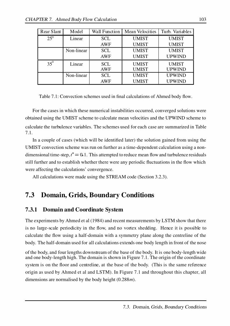
7/17/2019 Big
http://slidepdf.com/reader/full/big563db8d5550346aa9a975e13 120/189
CHAPTER 7. Ahmed Body Flow Calculation 103
Rear Slant Model Wall Function Mean Velocities Turb. Variables
25
Linear SCL UMIST UMIST
AWF UMIST UMIST
Non-linear SCL UMIST UMIST
AWF UMIST UPWIND
35 Linear SCL UMIST UMISTAWF UMIST UPWIND
Non-linear SCL UMIST UPWIND
AWF UMIST UPWIND
Table 7.1: Convection schemes used in final calculations of Ahmed body flow.
For the cases in which these numerical instabilities occurred, converged solutions were
obtained using the UMIST scheme to calculate mean velocities and the UPWIND scheme to
calculate the turbulence variables. The schemes used for each case are summarized in Table
7.1.
In a couple of cases (which will be identified later) the solution gained from using the
UMIST convection scheme was run on further as a time-dependent calculation using a non-
dimensional time-step, t 0 1. This attempted to reduce mean flow and turbulence residuals
still further and to establish whether there were any periodic fluctuations in the flow which
were affecting the calculations’ convergence.
All calculations were made using the STREAM code (Section 3.2.3).
7.3 Domain, Grids, Boundary Conditions
7.3.1 Domain and Coordinate System
The experiments by Ahmed et al (1984) and recent measurements by LSTM show that there
is no large-scale periodicity in the flow, and no vortex shedding. Hence it is possible to
calculate the flow using a half-domain with a symmetry plane along the centreline of the
body. The half-domain used for all calculations extends one body length in front of the nose
of the body, and four lengths downstream of the base of the body. It is one body-length wideand one body-length high. The domain is shown in Figure 7.1. The origin of the coordinate
system is on the floor and centreline, at the base of the body. (This is the same reference
origin as used by Ahmed et al and LSTM). In Figure 7.1 and throughout this chapter, all
dimensions are normalised by the body height (0.288m).
7.3. Domain, Grids, Boundary Conditions
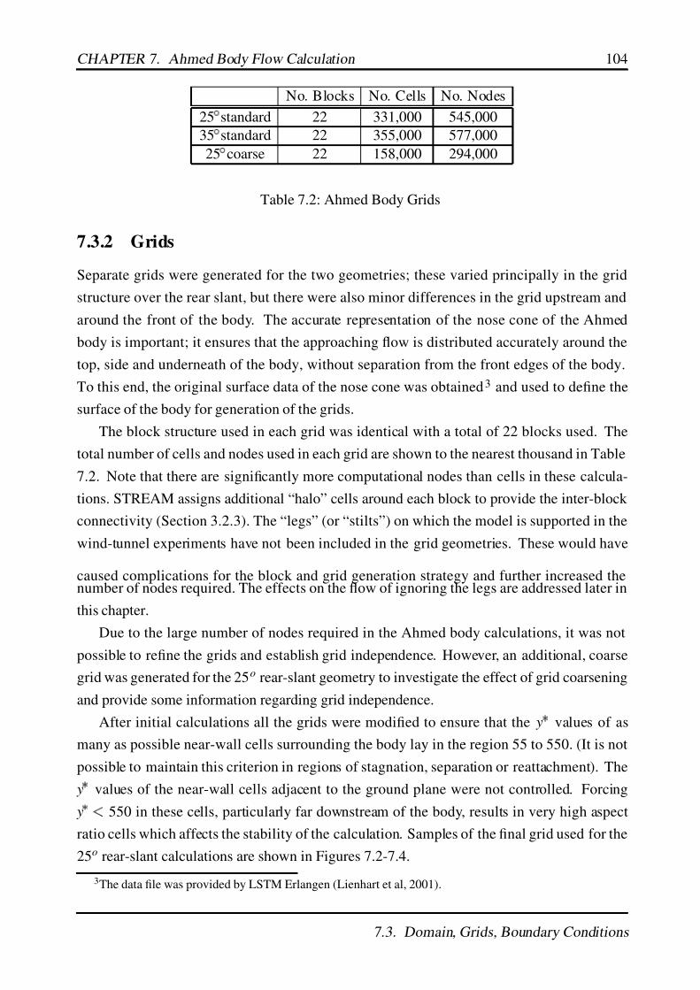
7/17/2019 Big
http://slidepdf.com/reader/full/big563db8d5550346aa9a975e13 121/189
CHAPTER 7. Ahmed Body Flow Calculation 104
No. Blocks No. Cells No. Nodes
25 standard 22 331,000 545,000
35
standard 22 355,000 577,000
25
coarse 22 158,000 294,000
Table 7.2: Ahmed Body Grids
7.3.2 Grids
Separate grids were generated for the two geometries; these varied principally in the grid
structure over the rear slant, but there were also minor differences in the grid upstream and
around the front of the body. The accurate representation of the nose cone of the Ahmed
body is important; it ensures that the approaching flow is distributed accurately around the
top, side and underneath of the body, without separation from the front edges of the body.
To this end, the original surface data of the nose cone was obtained3 and used to define the
surface of the body for generation of the grids.
The block structure used in each grid was identical with a total of 22 blocks used. The
total number of cells and nodes used in each grid are shown to the nearest thousand in Table
7.2. Note that there are significantly more computational nodes than cells in these calcula-
tions. STREAM assigns additional “halo” cells around each block to provide the inter-block
connectivity (Section 3.2.3). The “legs” (or “stilts”) on which the model is supported in the
wind-tunnel experiments have not been included in the grid geometries. These would have
caused complications for the block and grid generation strategy and further increased thenumber of nodes required. The effects on the flow of ignoring the legs are addressed later in
this chapter.
Due to the large number of nodes required in the Ahmed body calculations, it was not
possible to refine the grids and establish grid independence. However, an additional, coarse
grid was generated for the 25o rear-slant geometry to investigate the effect of grid coarsening
and provide some information regarding grid independence.
After initial calculations all the grids were modified to ensure that the y values of as
many as possible near-wall cells surrounding the body lay in the region 55 to 550. (It is not
possible to maintain this criterion in regions of stagnation, separation or reattachment). The
y values of the near-wall cells adjacent to the ground plane were not controlled. Forcing
y 550 in these cells, particularly far downstream of the body, results in very high aspect
ratio cells which affects the stability of the calculation. Samples of the final grid used for the
25o rear-slant calculations are shown in Figures 7.2-7.4.
3The data file was provided by LSTM Erlangen (Lienhart et al, 2001).
7.3. Domain, Grids, Boundary Conditions
7/17/2019 Big
http://slidepdf.com/reader/full/big563db8d5550346aa9a975e13 122/189
CHAPTER 7. Ahmed Body Flow Calculation 105
7.3.3 Boundary Conditions
The floor of the domain and the Ahmed body itself are treated as wall boundary conditions,
using either the simplified Chieng & Launder wall function (SCL) or analytical wall function
(AWF) described in Section 2.4. The domain boundary along the centreline of the body
( y
L 0 0), the opposite boundary at the outside limit of the domain ( y
L 3 625) and
the upper domain boundary ( z
L 3
625) were all treated as symmetry planes. Ideally the
upper domain boundary and domain boundary opposite the centre-plane would be treated
as “entrainment” boundaries. Symmetry planes were used instead to provide a more stable
calculation and are justifiable as there is very little deflection of the flow at these boundaries 4.
The downstream outlet is set with zero-gradient for all variables. At the upstream inlet,
pressure is set by linear extrapolation from the flow domain.
As STREAM is a non-dimensional code and the flow is incompressible, both the in-
let U -velocity and density are given the value 1
0. Viscosity is set by the inverse of theReynolds number and inlet values are specified for turbulent kinetic energy (k in
and tur-
bulence dissipation rate (εin). Profiles of velocity and normal stress 400mm in front of the
nose ( x
L
5 014 measured according to the coordinate system described in Section 7.3.1)
were provided by LSTM. As the calculated results were to be compared primarily to LSTM’s
measurements, these profiles were used to define the inlet Reynolds number and turbulence
values. The velocity profiles showed that at x
L
5 014 there was a deflection of the flow
due to the blockage effect of the body. This resulted in a lower mean U -velocity (38.51ms
1)
approaching the body across the height of the calculated domain than the experimental bulk
U -velocity (40.0ms
1 . The bulk Reynolds number for the calculation was adjusted accord-
ingly to Re 7 57x105 although the Reynolds number is sufficiently high that this minor
adjustment should not have significantly influenced the results.5
Inlet turbulent kinetic energy was calculated from LSTM’s normal stress profiles by:
k in
1
2
uu vv
ww (7.1)
The mean values of uu
vv
ww over the measured inlet profiles were used to calculate a
non-dimensional value for inlet turbulent kinetic energy: k in 4 39x10
6. Inlet turbulence
4Whereas a symmetry boundary condition applies zero gradient to all variables except the normal velocity
which is set to zero, the entrainment boundary condition sets zero gradient on all variables.5Ahmed et al (1984) used a bulk Reynolds number of Re
1 18x106 based on the body’s height for their
measurements.
7.3. Domain, Grids, Boundary Conditions

7/17/2019 Big
http://slidepdf.com/reader/full/big563db8d5550346aa9a975e13 123/189
CHAPTER 7. Ahmed Body Flow Calculation 106
dissipation rate was calculated by:
εin
c3 4
µ k 3 2
in
l(7.2)
The standard value of c µ 0 09 and, in the absence of any other data, an arbitrary value forl
0
07 L as suggested by Versteeg & Malalasekera (1996) were used. L is the reference
length used to calculate the Reynolds number of the flow - ie the height of the body. (In this
non-dimensional case, L 1 0). This provided a value: εin 2 16x10
8. It is somewhat
unrealistic to link the upstream dissipation rate to the dimensions of the body. However,
a cross-check was made by examining the turbulent to molecular viscosity ratio: νt
ν
60
which was thought to be a reasonable value. As LSTM had provided profiles at x
L
5 014
and the inlet was actually located at x
L
7 097, the inlet turbulence kinetic energy was
modified to k in 4
44x10
6 assuming a constant value of εin between the inlet and profile
locations. k in and εin were both set as flat profiles at the inlet.
At a later date, LSTM provided an estimate of the Taylor micro-scale of the flow upstream
of the body: λ 2
6mm, where the turbulence dissipation rate is defined:
ε
2k
λ2 ν (7.3)
The inlet dissipation rate was recalculated: εin 1 427x10
7 and the viscosity ratio: νt
ν
10.
This information was received too late in the project to implement the new boundary condi-
tion for all the calculations. It was used on one test calculation and shown to have no impacton the calculated flow around the body (demonstrated in Section 7.4.2).
7.4 25o Slant - Flow Field Results
7.4.1 Flow Upstream and Impinging on Body Nose
Upstream of the body, profiles of velocities and turbulent kinetic energy for three calcu-
lations (linear k ε /SCL; non-linear k ε /AWF; linear k ε /SCL/coarse grid) are shown
in Figures 7.5 and 7.6, compared to LSTM’s measured inlet data. The inlet profiles are at
x
L
5 014 - ie. 400mm in front of the body - and at three locations across the flow:
y
L 0 00 0 694 1 389. The location of the outside edge of the body is y
L 0 675.
The calculated profiles are all in good agreement with the measured data, providing con-
fidence that the inlet conditions and free-stream calculations are accurate. The U -velocity
profiles show the inviscid deflection of the flow, particularly on the centreline ( y
L 0
00)
7.4. 25 o Slant - Flow Field Results

7/17/2019 Big
http://slidepdf.com/reader/full/big563db8d5550346aa9a975e13 124/189
CHAPTER 7. Ahmed Body Flow Calculation 107
which is caused by the blockage effect of the body. The measured V -velocity on the cen-
treline shows a slight asymmetry in the flow, as there is a small measured amount of flow
across the y
L 0
00 plane. Naturally, this cannot be calculated as a symmetry condition is
imposed at the centreline.
Figures 7.7 to 7.9 show profiles for the same three calculations (linear k
ε /SCL; non-linear k ε /AWF; linear k ε /SCL/coarse grid) showing profiles of U and W -velocity and
turbulent kinetic energy on the centre-plane at various locations upstream and on the front
portion of the body. The velocity profiles all match the measured data well throughout this
region, with very little (if any) deviation between the calculations. The close agreement
between the standard and coarse grid calculations demonstrates grid independence in the
upstream region.
Differences between the linear and non-linear calculations become readily apparent in
the turbulent kinetic energy profiles (Figure 7.9). Both calculations which use the linear k ε
model show an increase in turbulent kinetic energy in the profile immediately upstream of
impingement ( x
L
3 7). This increased level of turbulent kinetic energy is convected
downstream and accounts for the high levels of turbulent kinetic energy near the surface of
the body in the last two profiles in Figure 7.9. The increase in turbulent kinetic energy is due
to the linear k ε model’s inability to calculate Pk accurately at impingement. This has been
discussed in detail for the case of flow around a square cylinder in Chapter 4.
Two sets of LSTM’s measured data are shown in Figure 7.9. The triangles show LDA
measurements which were made on the centre-plane whereas the crosses show the upstream
data which was measured using HWA in a separate experiment. These two datasets shareone common location: x
L
5 014; y
L 0
00. The data shown as triangles (centre-plane
data) is about an order of magnitude greater than that shown as crosses (upstream profiles) at
this location. Lienhart et al (2001) attribute the differences in the measured turbulent kinetic
energy to the different measurement techniques used. LDA is better suited to measurements
in highly turbulent regions, including reverse flow, whereas HWA is better suited to regions
of low turbulence. Upstream of the body, there is little turbulence in the flow and the HWA
measurements will be more accurate than the LDA measurements. The calculations are in
better agreement with the HWA data.
The flow upstream of the body, at impingement and on the front section of the body
is essentially inviscid. This is shown by the close agreement between the velocity profiles
for the different calculations despite the different turbulence models used and differences in
calculated turbulent kinetic energy.
7.4. 25 o Slant - Flow Field Results
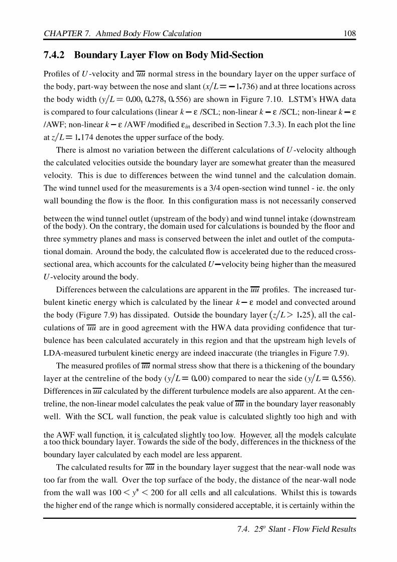
7/17/2019 Big
http://slidepdf.com/reader/full/big563db8d5550346aa9a975e13 125/189
CHAPTER 7. Ahmed Body Flow Calculation 108
7.4.2 Boundary Layer Flow on Body Mid-Section
Profiles of U -velocity and uu normal stress in the boundary layer on the upper surface of
the body, part-way between the nose and slant ( x
L
1 736) and at three locations across
the body width ( y
L 0 00 0 278 0 556) are shown in Figure 7.10. LSTM’s HWA data
is compared to four calculations (linear k ε /SCL; non-linear k ε /SCL; non-linear k ε
/AWF; non-linear k ε /AWF /modified εin described in Section 7.3.3). In each plot the line
at z
L 1
174 denotes the upper surface of the body.
There is almost no variation between the different calculations of U -velocity although
the calculated velocities outside the boundary layer are somewhat greater than the measured
velocity. This is due to differences between the wind tunnel and the calculation domain.
The wind tunnel used for the measurements is a 3/4 open-section wind tunnel - ie. the only
wall bounding the flow is the floor. In this configuration mass is not necessarily conserved
between the wind tunnel outlet (upstream of the body) and wind tunnel intake (downstreamof the body). On the contrary, the domain used for calculations is bounded by the floor and
three symmetry planes and mass is conserved between the inlet and outlet of the computa-
tional domain. Around the body, the calculated flow is accelerated due to the reduced cross-
sectional area, which accounts for the calculated U velocity being higher than the measured
U -velocity around the body.
Differences between the calculations are apparent in the uu profiles. The increased tur-
bulent kinetic energy which is calculated by the linear k ε model and convected around
the body (Figure 7.9) has dissipated. Outside the boundary layer
z
L 1
25 , all the cal-
culations of uu are in good agreement with the HWA data providing confidence that tur-
bulence has been calculated accurately in this region and that the upstream high levels of
LDA-measured turbulent kinetic energy are indeed inaccurate (the triangles in Figure 7.9).
The measured profiles of uu normal stress show that there is a thickening of the boundary
layer at the centreline of the body ( y
L 0 00) compared to near the side ( y
L 0 556).
Differences in uu calculated by the different turbulence models are also apparent. At the cen-
treline, the non-linear model calculates the peak value of uu in the boundary layer reasonably
well. With the SCL wall function, the peak value is calculated slightly too high and with
the AWF wall function, it is calculated slightly too low. However, all the models calculatea too thick boundary layer. Towards the side of the body, differences in the thickness of the
boundary layer calculated by each model are less apparent.
The calculated results for uu in the boundary layer suggest that the near-wall node was
too far from the wall. Over the top surface of the body, the distance of the near-wall node
from the wall was 100
y
200 for all cells and all calculations. Whilst this is towards
the higher end of the range which is normally considered acceptable, it is certainly within the
7.4. 25 o Slant - Flow Field Results
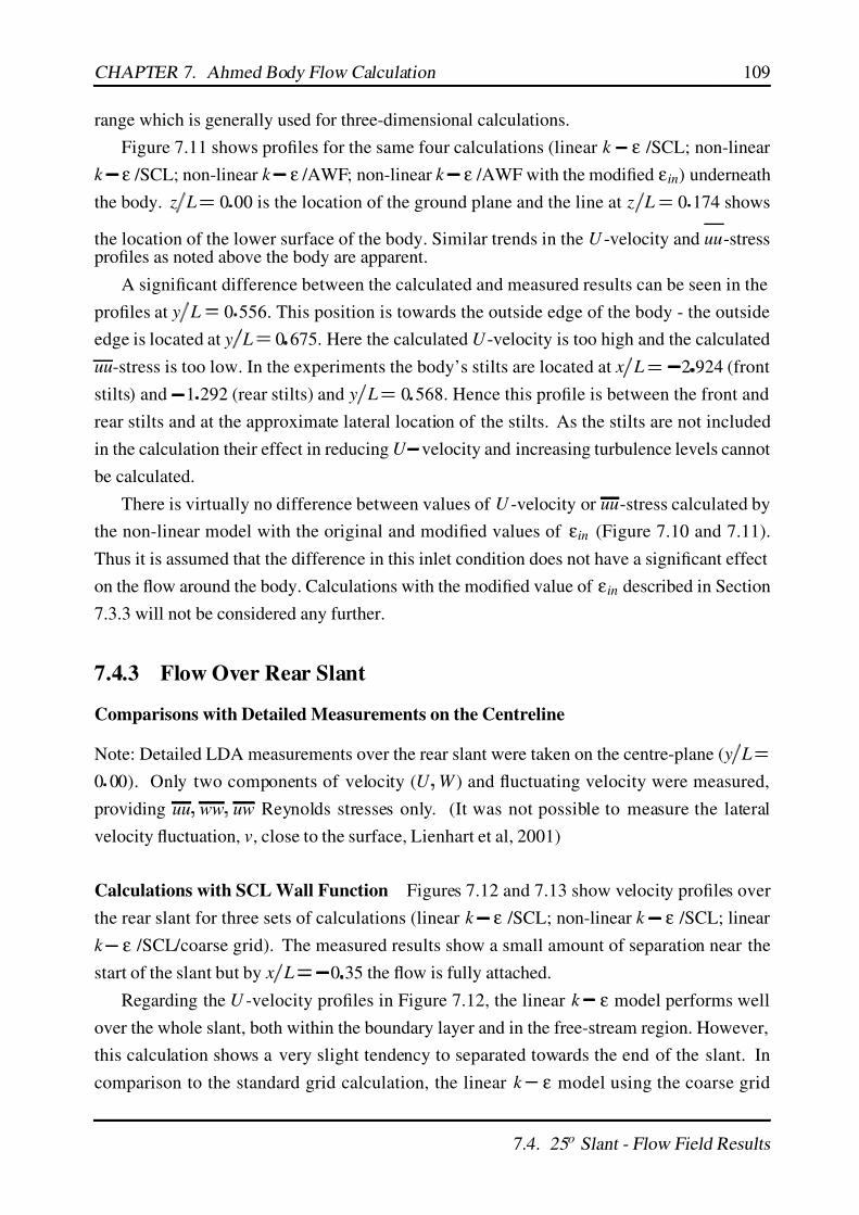
7/17/2019 Big
http://slidepdf.com/reader/full/big563db8d5550346aa9a975e13 126/189
CHAPTER 7. Ahmed Body Flow Calculation 109
range which is generally used for three-dimensional calculations.
Figure 7.11 shows profiles for the same four calculations (linear k ε /SCL; non-linear
k ε /SCL; non-linear k ε /AWF; non-linear k ε /AWF with the modified εin) underneath
the body. z
L 0 00 is the location of the ground plane and the line at z
L 0 174 shows
the location of the lower surface of the body. Similar trends in the U -velocity and uu-stressprofiles as noted above the body are apparent.
A significant difference between the calculated and measured results can be seen in the
profiles at y
L 0 556. This position is towards the outside edge of the body - the outside
edge is located at y
L 0
675. Here the calculated U -velocity is too high and the calculated
uu-stress is too low. In the experiments the body’s stilts are located at x
L
2 924 (front
stilts) and 1 292 (rear stilts) and y
L 0
568. Hence this profile is between the front and
rear stilts and at the approximate lateral location of the stilts. As the stilts are not included
in the calculation their effect in reducing U velocity and increasing turbulence levels cannot
be calculated.
There is virtually no difference between values of U -velocity or uu-stress calculated by
the non-linear model with the original and modified values of εin (Figure 7.10 and 7.11).
Thus it is assumed that the difference in this inlet condition does not have a significant effect
on the flow around the body. Calculations with the modified value of εin described in Section
7.3.3 will not be considered any further.
7.4.3 Flow Over Rear Slant
Comparisons with Detailed Measurements on the Centreline
Note: Detailed LDA measurements over the rear slant were taken on the centre-plane ( y
L
0 00). Only two components of velocity (U W ) and fluctuating velocity were measured,
providing uu ww
uw Reynolds stresses only. (It was not possible to measure the lateral
velocity fluctuation, v, close to the surface, Lienhart et al, 2001)
Calculations with SCL Wall Function Figures 7.12 and 7.13 show velocity profiles over
the rear slant for three sets of calculations (linear k ε /SCL; non-linear k ε /SCL; linear
k ε /SCL/coarse grid). The measured results show a small amount of separation near the
start of the slant but by x
L
0 35 the flow is fully attached.
Regarding the U -velocity profiles in Figure 7.12, the linear k ε model performs well
over the whole slant, both within the boundary layer and in the free-stream region. However,
this calculation shows a very slight tendency to separated towards the end of the slant. In
comparison to the standard grid calculation, the linear k ε model using the coarse grid
7.4. 25 o Slant - Flow Field Results

7/17/2019 Big
http://slidepdf.com/reader/full/big563db8d5550346aa9a975e13 127/189
CHAPTER 7. Ahmed Body Flow Calculation 110
performs slightly less well in the boundary layer on the first half of the slant. On the latter
half of the slant, the flow calculated with the the coarse grid shows less tendency to separate
than the standard grid calculation. Refining the grid improves the calculated flow on the
upper half of the slant, but appears to worsen it on the lower half. Apparently, in this region
the “artificial viscosity” induced by the coarse grid helps maintain attached flow.The non-linear k ε model performs much less well than the linear k ε model; there is
a large amount of separation along virtually the whole slant. Separation is initially calculated
by the non-linear model near the start of the slant which is also apparent in the measurements.
However, instead of reattachment occurring by x
L
0 35 (as the measurements show),
the separation region grows. The excessive amount of separation calculated by the non-linear
model is similar to that observed for the square cylinder described in Chapter 4.
The W -velocity profiles in Figure 7.13 show the same trends as are seen for the U -velocity
profiles. The linear k ε calculation performs well; the non-linear k ε calculation performs
less well. Due to the large separated flow region calculated by the non-linear model, the
velocity vectors are nearly horizontal. Consequently, the magnitude of the W -velocity is
much smaller than that calculated by the linear model.
Three Reynolds stresses (uu
ww
uw) are shown in Figures 7.14 to 7.16 respectively. For
all three sets of calculations, the Reynolds stresses are not well predicted, which goes some
way to explaining the tendency to calculate flow separation towards the end of the slant. The
measurements show a large amount of Reynolds stress generated between x
L
0 64 and
0 50 due to the shear layer originating at the start of the slant. The high Reynolds stress is
convected downstream and gradually dissipates towards the end of the slant.Figure 7.10 shows that both the linear and non-linear k ε models calculate the stream-
wise normal stress (uu) reasonably accurately in the boundary layer over the top of the body
(certainly to the correct order of magnitude). It is peculiar that there should develop so rapidly
an order of magnitude difference between the measured and calculated Reynolds stresses at
the start of the slant. It is also hard to imagine that the linear k ε model can calculate such a
good agreement with the measured velocity profiles if the computed shear stress is so much
in error.
In an attempt to understand this better, comparison is made to a simpler flow in an adverse
pressure gradient. In Table 7.3 comparison is made of the approximate values of maximum
normalised Reynolds stresses6 which have been measured in the 10o plane diffuser (Chapter
6: Figures 6.10 to 6.12) with the values measured over the rear slant of the Ahmed body
(Figures 7.14 to 7.16). For all the stresses, the values measured over the rear slant of the
6The vertical direction in the plane diffuser is the y-direction and z-direction in the Ahmed body hence
vv Di f f user equates to ww Ahmed etc.
7.4. 25 o Slant - Flow Field Results
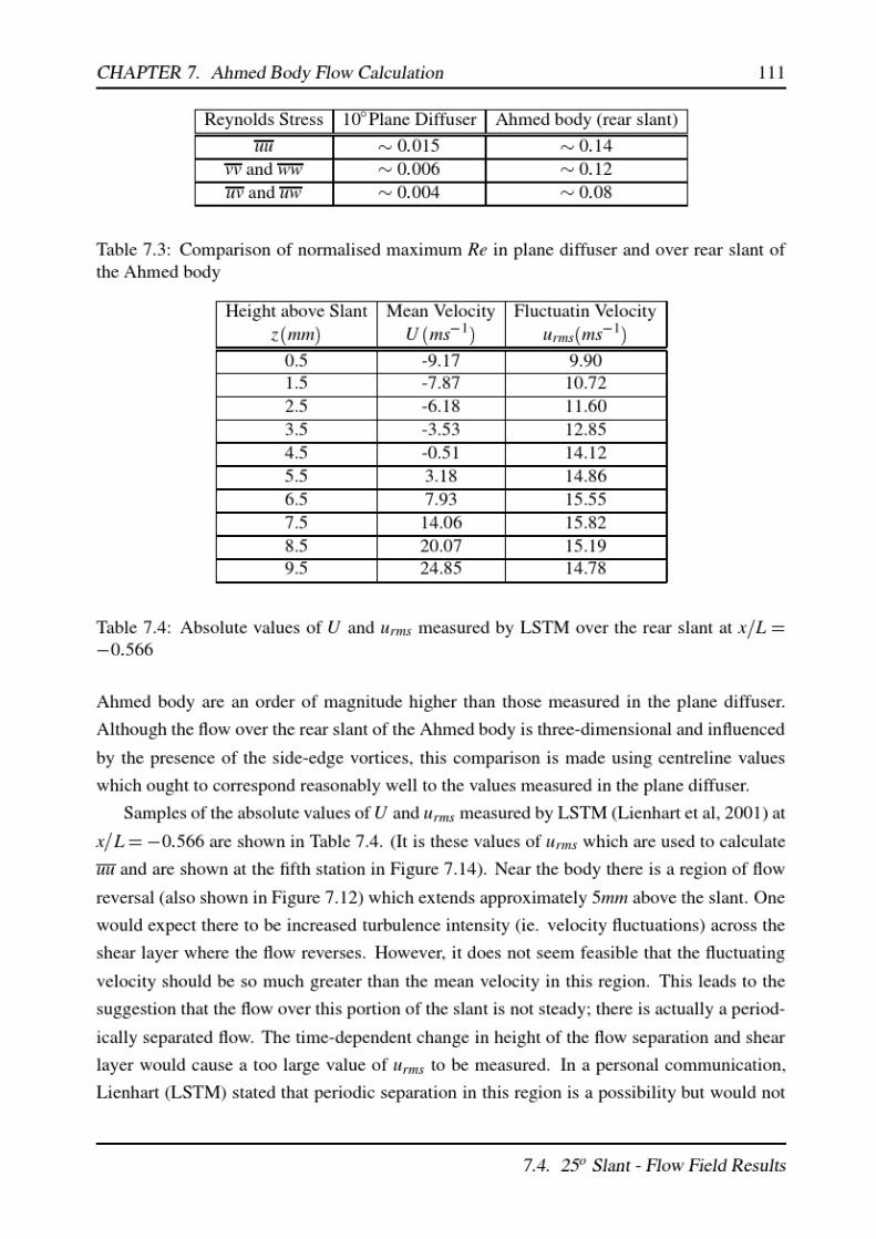
7/17/2019 Big
http://slidepdf.com/reader/full/big563db8d5550346aa9a975e13 128/189
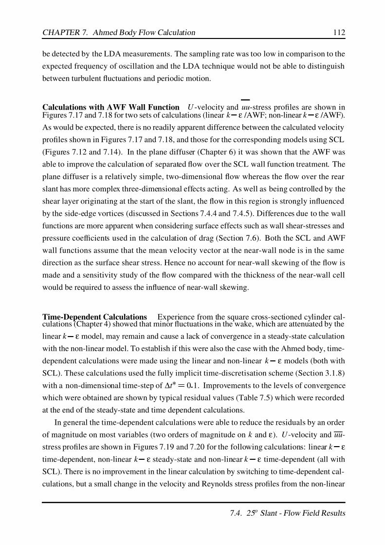
7/17/2019 Big
http://slidepdf.com/reader/full/big563db8d5550346aa9a975e13 129/189
CHAPTER 7. Ahmed Body Flow Calculation 112
be detected by the LDA measurements. The sampling rate was too low in comparison to the
expected frequency of oscillation and the LDA technique would not be able to distinguish
between turbulent fluctuations and periodic motion.
Calculations with AWF Wall Function U -velocity and uu-stress profiles are shown inFigures 7.17 and 7.18 for two sets of calculations (linear k ε /AWF; non-linear k ε /AWF).
As would be expected, there is no readily apparent difference between the calculated velocity
profiles shown in Figures 7.17 and 7.18, and those for the corresponding models using SCL
(Figures 7.12 and 7.14). In the plane diffuser (Chapter 6) it was shown that the AWF was
able to improve the calculation of separated flow over the SCL wall function treatment. The
plane diffuser is a relatively simple, two-dimensional flow whereas the flow over the rear
slant has more complex three-dimensional effects acting. As well as being controlled by the
shear layer originating at the start of the slant, the flow in this region is strongly influenced
by the side-edge vortices (discussed in Sections 7.4.4 and 7.4.5). Differences due to the wall
functions are more apparent when considering surface effects such as wall shear-stresses and
pressure coefficients used in the calculation of drag (Section 7.6). Both the SCL and AWF
wall functions assume that the mean velocity vector at the near-wall node is in the same
direction as the surface shear stress. Hence no account for near-wall skewing of the flow is
made and a sensitivity study of the flow compared with the thickness of the near-wall cell
would be required to assess the influence of near-wall skewing.
Time-Dependent Calculations Experience from the square cross-sectioned cylinder cal-culations (Chapter 4) showed that minor fluctuations in the wake, which are attenuated by the
linear k ε model, may remain and cause a lack of convergence in a steady-state calculation
with the non-linear model. To establish if this were also the case with the Ahmed body, time-
dependent calculations were made using the linear and non-linear k ε models (both with
SCL). These calculations used the fully implicit time-discretisation scheme (Section 3.1.8)
with a non-dimensional time-step of ∆t 0 1. Improvements to the levels of convergence
which were obtained are shown by typical residual values (Table 7.5) which were recorded
at the end of the steady-state and time dependent calculations.
In general the time-dependent calculations were able to reduce the residuals by an order
of magnitude on most variables (two orders of magnitude on k and ε). U -velocity and uu-
stress profiles are shown in Figures 7.19 and 7.20 for the following calculations: linear k ε
time-dependent, non-linear k ε steady-state and non-linear k ε time-dependent (all with
SCL). There is no improvement in the linear calculation by switching to time-dependent cal-
culations, but a small change in the velocity and Reynolds stress profiles from the non-linear
7.4. 25 o Slant - Flow Field Results
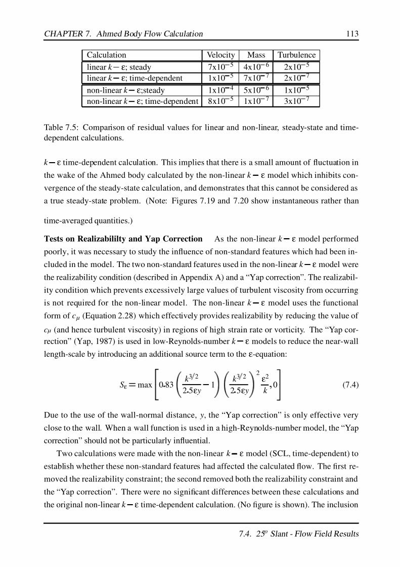
7/17/2019 Big
http://slidepdf.com/reader/full/big563db8d5550346aa9a975e13 130/189
CHAPTER 7. Ahmed Body Flow Calculation 113
Calculation Velocity Mass Turbulence
linear k ε; steady 7x10
5 4x10
6 2x10
5
linear k ε; time-dependent 1x10
5 7x10
7 2x10
7
non-linear k ε;steady 1x10
4 5x10
6 1x10
5
non-linear k ε; time-dependent 8x10
5 1x10
7 3x10
7
Table 7.5: Comparison of residual values for linear and non-linear, steady-state and time-
dependent calculations.
k ε time-dependent calculation. This implies that there is a small amount of fluctuation in
the wake of the Ahmed body calculated by the non-linear k ε model which inhibits con-
vergence of the steady-state calculation, and demonstrates that this cannot be considered as
a true steady-state problem. (Note: Figures 7.19 and 7.20 show instantaneous rather than
time-averaged quantities.)
Tests on Realizabililty and Yap Correction As the non-linear k ε model performed
poorly, it was necessary to study the influence of non-standard features which had been in-
cluded in the model. The two non-standard features used in the non-linear k ε model were
the realizability condition (described in Appendix A) and a “Yap correction”. The realizabil-
ity condition which prevents excessively large values of turbulent viscosity from occurring
is not required for the non-linear model. The non-linear k ε model uses the functional
form of c µ (Equation 2.28) which effectively provides realizability by reducing the value of
c µ (and hence turbulent viscosity) in regions of high strain rate or vorticity. The “Yap cor-
rection” (Yap, 1987) is used in low-Reynolds-number k ε models to reduce the near-wall
length-scale by introducing an additional source term to the ε-equation:
S ε max
0 83
k 3 2
2 5ε y
1
k 3 2
2 5ε y
2
ε2
k 0
(7.4)
Due to the use of the wall-normal distance, y, the “Yap correction” is only effective very
close to the wall. When a wall function is used in a high-Reynolds-number model, the “Yap
correction” should not be particularly influential.
Two calculations were made with the non-linear k ε model (SCL, time-dependent) to
establish whether these non-standard features had affected the calculated flow. The first re-
moved the realizability constraint; the second removed both the realizability constraint and
the “Yap correction”. There were no significant differences between these calculations and
the original non-linear k ε time-dependent calculation. (No figure is shown). The inclusion
7.4. 25 o Slant - Flow Field Results
7/17/2019 Big
http://slidepdf.com/reader/full/big563db8d5550346aa9a975e13 131/189
CHAPTER 7. Ahmed Body Flow Calculation 114
of the realizability constraint and “Yap correction” did not adversely effect the non-linear
k ε calculation.
Tests on Convection Scheme Initial calculations were made with the first-order UPWIND
convection scheme to establish the basic flow pattern before switching to the higher-orderUMIST convection scheme. Little difference in the flow around the body was noted with the
linear k ε model when switching between the UPWIND and UMIST convection schemes.
There was however, a marked difference when the non-linear k ε model was used.
Figure 7.21 shows U -velocity profiles for the steady-state linear k ε /UMIST, non-linear
k ε /UMIST and non-linear k ε /UPWIND calculations. Being only first-order accurate,
the UPWIND scheme is more diffusive than the UMIST scheme, adding artificial viscosity
to the flow. Hence the flow calculated by the non-linear model and UPWIND scheme re-
mains attached at the start of the slant, whereas the non-linear model and UMIST scheme
calculates a small separation. More significantly, the flow calculated by the non-linear model
and UPWIND scheme remains attached along the whole length of the slant, whereas with the
UMIST scheme it is separated.
The UMIST convection scheme is formally more accurate than the UPWIND scheme.
This comparison is made to demonstrate the action of viscosity (“real” or “artificial”) on
the flow over the slant, rather than to advocate the use of first-order convection schemes. In
Chapter 1 the critical influence of the side-edge vortices on determining whether the flow over
the slant separates is discussed. To help explain these differences, the formation of this vortex
due to mean strain bending is discussed in Section 7.4.4 with reference to the calculation of vorticity and mean strain bending by the different turbulence models and convection schemes.
Sensitivity to c µ and Non-Linear Components of Reynolds Stresses The two features of
the non-linear k ε model of Craft et al (1996b) which make it different from the standard
linear k ε model of Launder & Spalding (1974) are the functional form of c µ (Equation 2.28)
and the inclusion of the non-linear components in the Reynolds stresses (Equation 2.27). To
establish whether one or other of these features were responsible for the separated flow over
the rear slant, two tests were made. Firstly, the c µ function was modified to the form which
is effectively used in the linear k ε model when the realizability condition is employed
(Equation A.30). This form of the function does not reduce c µ so greatly in regions of high
S or Ω as shown in Figure 2.1. Secondly, the original c µ function proposed by Craft et al
(1996b) was retained, and the non-linear components were set to zero.
The U -velocity profiles over the rear slant calculated by the two modified models are
shown in Figures 7.22 (modified c µ) and Figure 7.23 (uiu j NL 0). For each modification
7.4. 25 o Slant - Flow Field Results

7/17/2019 Big
http://slidepdf.com/reader/full/big563db8d5550346aa9a975e13 132/189
CHAPTER 7. Ahmed Body Flow Calculation 115
there is a small improvement in the calculated velocity profiles, but neither modification
calculates attached flow along the slant. It would appear that either the original form of c µ
or the inclusion of the non-linear components in the Reynolds stresses alone, is sufficient to
cause the flow to separate over the slant.
Comparisons with Measurements in the Wake and off the Centreline
LSTM have taken LDA measurements of mean and fluctuating velocity components for a
number of profiles on the wake of the Ahmed body and off-centreline. These lie in planes
between the centreline and the outside edge of the body: y
L 0
00
0
347
0
625 and 0
675.
(This last plane being the plane of the outside edge of the body.) In general these confirm the
results discussed in Section 7.4.3.1, and only a brief selection is now shown.
Figures 7.24 and 7.25 show U and W -velocity profiles on the centreline compared to
the LDA masurements. Calculated values from the linear and non-linear k
ε models areshown both using the SCL wall function and higher order UMIST convection scheme. (Figure
7.24 is essentially the same as Figure 7.12 but extended into the wake.) The U -velocity
profiles in Figure 7.24 show that the linear k ε model calculates the mean velocity more
accurately than the non-linear model in the wake, as well as over the slant. The non-linear
model calculates U -velocity profiles in the wake similar to those seen in the wake of the
square cylinder (Chapter 4): the recirculation region is too high in the z-direction and the
magnitude of the reverse velocity is too low.
Reynolds normal and shear stresses (uu and uw) are shown at the same locations as the
velocities in Figures 7.26 and 7.27. Over the rear section of the slant, the linear k ε model
calculates the correct shape of the distribution of uu and uw, although the magnitudes of the
Reynolds stresses are too low. The non-linear model calculates a separated flow in this region
and the peak in the Reynolds stresses above the slant is due to the shear layer in the region of
the separation streamline.
Figures 7.28 to 7.30 show profiles of U , V and W -velocity for the same two models at
y
L 0 625 (near the outer edge). The notable feature is the near-wall “bulge” in the U -
velocity profiles towards the end (Figure 7.28) and the more vigorous motion shown by the
V -velocity profiles (Figure 7.29). These indicate the presence of the side-edge vortex. Again,the linear k ε model calculates this feature more accurately than the non-linear model,
although the magnitude of the calculated V -velocity is too low, probably due to the use of
wall functions. Formation of the side-edge vortex is discussed in Section 7.4.4. Reynolds
stresses (uu and uw) are shown in Figures 7.31 and 7.32. In general the Reynolds stresses
are much lower towards the side of the body than at the centreline. The non-linear model
calculates levels of Reynolds stress in the wake at y
L 0
625 slightly better than the linear
7.4. 25 o Slant - Flow Field Results
7/17/2019 Big
http://slidepdf.com/reader/full/big563db8d5550346aa9a975e13 133/189
CHAPTER 7. Ahmed Body Flow Calculation 116
model.
7.4.4 Vortex Formation
It is known that the occurrence of attached or separated flow on the rear slant of the Ahmed
body is strongly influenced by the formation of the side-edge vortex (Ahmed et al, 1984).
From the results discussed so far in Chapter 7, it is apparent that the calculation of separated
or attached flow, and consequently the calculation of the side-edge vortex, is dependent upon
the turbulence model and convection scheme used. To help understand the formation of the
vortex, it is useful to consider the equation for streamwise vorticity, Ω x:
DΩ x
Dt
(7.5)
In the above, vorticity components are Ω x ∂V
∂ z ∂W
∂ y
, Ω y ∂W
∂ x ∂U
∂ z
and Ω z ∂U
∂ y ∂V
∂ x
The principal source term for the streamwise vorticity is the mean strain bending. There will
also be contributions from turbulent normal stress and turbulent shear stress generation in
the non-linear k ε model (which are zero in a linear model). Figure 7.33 shows the mean
strain bending at the start of the slant ( x
L
0 701) calculated by the linear k ε model,
and the non-linear k ε model using the UMIST and UPWIND convection schemes. Both
the linear model and the non-linear model/UPWIND calculate higher values of mean strain
bending than the non-linear model/UMIST. Figure 7.34 shows the calculated mean strain
bending half-way along the slant ( x
L
0
347). Here, the difference is more marked withthe non-linear model/UMIST calculating significantly less mean strain bending than the other
two models.
As a relatively high value of the source term for streamwise vorticity is calculated by
the linear model and non-linear model/UPWIND, these two models calculate more stream-
wise vorticity than the non-linear model/UMIST computation. Figures 7.35, 7.36 and 7.37
show the calculated streamwise vorticity for the three models at the start of the slant ( x
L
0 701), half-way along the slant ( x
L
0 347) and at the end of the slant/base
x
L
0 00). It is apparent that, despite calculating separated flow over a large portion of the rear
slant, the non-linear k ε model/UMIST does calculate a well defined side-edge vortex. At
the end of the slant (Figure 7.37) the vortex calculated by the non-linear model with the higher
order UMIST scheme is almost as strong as that calculated using the UPWIND scheme, al-
though it is less diffuse. The stronger vortex calculated by the linear k ε model and the
diffuse vortex calculated by the non-linear model/UPWIND draw fluid out of the boundary
layer on the slant near the centreline of the the body. This is sufficient to maintain attached
7.4. 25 o Slant - Flow Field Results
7/17/2019 Big
http://slidepdf.com/reader/full/big563db8d5550346aa9a975e13 134/189
CHAPTER 7. Ahmed Body Flow Calculation 117
flow over the slant. In contrast, the weak and well-defined vortex calculated by the non-linear
model/UMIST does not draw a sufficient amount of fluid out of the boundary layer and the
flow separates.
To help visualise the region of attached flow and influence of the side-edge vortex, Figure
7.38 shows velocity vectors calculated at the near-wall nodes by the linear k
ε model andnon-linear k ε model/UMIST. (The top surface and slant are shown viewed from above with
the side of the body “unfolded”.) The separated (reversed) flow calculated by the non-linear
model/UMIST extends across most of the rear slant with only a small region of attached flow
near the side edge, due to the influence of the vortex.
7.4.5 Wake
Secondary velocity vectors in the wake are shown at three planes downstream of the body
( x
L 0 277 0 694 1 736) for the linear k
ε model (SCL/steady) in Figure 7.39 and for
the non-linear k ε model (SCL/steady) in Figure 7.40 (both using the UMIST scheme).
These figures show the outline of the Ahmed body and location of the rear edge of the slant.
Calculated vectors are shown in the right half-plane with LSTM measured vectors reflected
onto the left half-plane.
The secondary vectors calculated by the linear model in Figure 7.39 show good develop-
ment of the wake-vortex, both in terms of its position and magnitude. Flow across the lower
half of the base of the body ( x
L 0 277) which is associated with the horseshoe vortices
(Figures 1.13 and 1.14) is not calculated. The wake vortex develops from the side-edge vortex
which is discussed in Section 7.4.4. When the flow is calculated with the non-linear model,
a relatively weak side-edge vortex is calculated which is confined to a narrow region at the
side edge of the slant. Figure 7.40 shows how the lack of a strong side-edge vortex in the
non-linear calculation affects the wake. The non-linear model calculates a small amount of
downwash in the wake at x
L 0 277 and 0.694 but the strong wake-vortex which is mea-
sured by LSTM and calculated by the linear model does not appear. At x
L 1 736 the large
measured vortex is calculated by the non-linear model but not so well as it is calculated by
the linear model.
In Section 7.4.3.1 and Figure 7.21 it is shown that by reverting to the first-order, diffusive,UPWIND convection scheme with the non-linear k ε model, an attached flow over the slant
could be calculated. This then produces a strong side-edge vortex (Figures 7.35 to 7.37)
which develops the wake vortex shown in Figure 7.41. The strong wake-vortex which is
calculated by the non-linear/UPWIND model is, in general, in as good agreement with the
measurements as the linear model with the UMIST convection scheme. This demonstrates
the effectiveness of the non-linear terms in the stress-strain relationship (Equation 2.27) in
7.4. 25 o Slant - Flow Field Results
7/17/2019 Big
http://slidepdf.com/reader/full/big563db8d5550346aa9a975e13 135/189
CHAPTER 7. Ahmed Body Flow Calculation 118
improving flow with streamwise vorticity, albeit with a first-order convection scheme.
Development of turbulent kinetic energy in the wake is shown for the same three calcu-
lations: linear/UMIST, non-linear/UMIST, non-linear/UPWIND (all using SCL) in Figures
7.42 to 7.44 respectively. None of the calculated turbulent kinetic energy plots show the
peaks in the turbulent kinetic energy at the centre of the vortex at the rear edge of the slant( x
L 0
277). The linear/UMIST calculation reproduces the shape and magnitude of the tur-
bulent kinetic energy contours reasonably well (Figure 7.42); this is slightly improved upon
by the non-linear/UPWIND calculation (Figure 7.44). As would be expected from the poor
calculation of the wake secondary-velocity, the non-linear/UMIST calculation of turbulent
kinetic energy is also poor (Figure 7.43).
7.4.6 Pressure on Base and Slant
Coefficient of pressure (C P) contours on the surface of the body’s base and rear slant are
shown in Figures 7.45 and 7.46 for the linear k ε model (SCL, AWF) and non-linear k ε
model (SCL, AWF) calculations. Measured coefficient of pressure is shown on the left half
of the body and calculated pressure on the right half for each case. Rather than showing the
slant in projection, it has been “unfolded” hence the base and slant have different z
L scales.
Coefficient of pressure is calculated by:
C P
P P0
0 5ρU 2o
(7.6)
where Po is the pressure at a reference point in the flow, ρ is the density and U o is the upstream
(undisturbed) velocity used in the calculation of Reynolds number.
For the linear k ε calculations, Figure 7.45 shows the effect of the side-edge vortex
on C P contours at the right-hand edge of the slant. The pressure gradient shown by these
contours is not so great as the pressure gradient due to the measured side-edge vortex (left-
hand edge), indicating that the calculated vortex is not as strong as the measured vortex.
Conversely, the calculated pressure gradient at the top edge (start) of the slant is much greater
than the measured pressure gradient. Although the shape of the calculated C P plot is similar
to the measured data, the differences in the magnitude of C P will effect the accuracy of thecalculated drag. There is a very minor improvement in the calculation of pressure when using
the AWF wall function. Across the base of the body there is little variation in the measured
or calculated coefficients of pressure, indicating that the flow is quiescent in this region.
C P
0 190 across the base for the measured and both calculated sets.
The separated flow calculated by the non-linear/UMIST model is evident from relatively
small change in C P along the slant (Figure 7.46). The weak vortex which is calculated has
7.4. 25 o Slant - Flow Field Results
7/17/2019 Big
http://slidepdf.com/reader/full/big563db8d5550346aa9a975e13 136/189
CHAPTER 7. Ahmed Body Flow Calculation 119
a small effect on the contours at the right-hand edge. C P calculated using the non-linear
model and AWF does not show the weak vortex. When using the AWF wall function with the
non-linear model it was not possible to use the UMIST convection scheme to calculate both
the mean velocities and turbulence values as was used with the SCL wall function (Section
7.2). Instead, the UMIST scheme was used for the mean velocities and the UPWIND schemefor the turbulence variables (Table 7.1). Subsequently the calculated side-edge vortex is not
strong enough to show any effect on the calculated C P over the slant. The calculation of base
pressure is improved slightly by using the AWF rather than the SCL wall function. (On the
base the flow is fully separated and both the linear and non-linear models calculate separated
flow here).
7.5 35o Slant - Flow Field Results
7.5.1 Flow Over Rear Slant and In Wake
For the Ahmed body with the 35o rear-slant angle, flow is fully separated over the slant
and strong side-edge vortices do not form (Ahmed et al, 1984, Lienhart et al, 2001). The
measured data used in this section to assess the calculated results is from a preliminary study
by Lienhart et al (2001). There is less data available than for the body with the 25o rear slant
and it was released before consistency checks had been carried out.
Calculations with the SCL Wall Function Figure 7.47 to 7.49 show the U and W -velocityprofiles and turbulent kinetic energy profiles on the centreline for LSTM’s measured data
and two calculations: linear k ε and non-linear k ε both using the SCL wall function.
Although the data is a lot more sparse for the 35 o case, it is clear that both the linear and
non-linear models calculate separated flow over the body’s rear slant in accordance with the
measurements (Figure 7.47).
The calculated wake flow is similar to that behind the square cross-sectioned cylinder
(Chapter 4). The linear k ε model calulates the shape of the U and W -velocity profiles well
and the length of the recirculating flow region is calculated reasonably accurately by this
model. As was seen with the square cylinder, the non-linear model calculates a recirculation
region which is too high ( z-direction) and too long ( x-direction). The U -velocity gradients
calculated by the non-linear model in the upper and lower shear layers are too steep.
Both the linear and non-linear k ε models calculate too much turbulent kinetic energy in
the wake (Figure 7.49). In the lower shear layer of the wake and close to the body, the turbu-
lent kinetic energy ought to be similar for calculations with the 25 o and 35o slants. (Here, the
7.5. 35 o Slant - Flow Field Results
7/17/2019 Big
http://slidepdf.com/reader/full/big563db8d5550346aa9a975e13 137/189
CHAPTER 7. Ahmed Body Flow Calculation 120
Data 25
Rear Slant 35
Rear Slant
Measured
0 10
0 015
Calculated by linear k εmodel
0 07
0 08
Calculated by non-linear k εmodel
0.05
0 04
Table 7.6: Measured and claculated values of k in the lower shear layer close to the base of
the Ahmed body with 25o and 35o rear slants.
flow is relatively unaffected by the behaviour of the flow over the slant.) Measured data is not
available at the same locations in the wake for the 25o and 35o bodies. Instead, a comparison
is made of turbulent kinetic energy at x
L
0 3 for the 25o rear-slant body (Figure 7.50)
and x
L
0 5 for the 35o rear-slant body (Figure 7.49); measured and calculated values of
turbulent kinetic energy are shown in Table 7.6:
Although there is reasonable agreement in the calculated turbulent kinetic energy betweenthe 25o and 35o bodies when using either turbulence model, there is a considerable difference
in the levels of measured turbulent kinetic energy. It is worth re-iterating that the measured
data provided by LSTM for the 35o body (Lienhart et al, 2001) was preliminary data, which
was issued before the measurements were completed in full and before consistency checks
were made. Without the complete 35o rear-slant measured dataset and a full study of the
calculated versus measured data, it is not possible to judge the accuracy of the calculated
turbulent kinetic energy.
Calculations with AWF Wall Function Calculated profiles of U -velocity and turbulent
kinetic energy using the AWF wall function are shown in Figures 7.51 and 7.52. As would
be expected the change in the wall treatment has little effect on the wake flow, which is dom-
inated by free-stream effects. The minor differences that do occur (for example, in the linear
calculation of the U -velocity profile at x
L
1 77) are due to time-dependent fluctuations
in the wake, which in this steady-state calculation are manifested as minor differences in the
level of convergence.
Tests on Realizabililty and Yap Correction Han (1989) was not able to calculate a sepa-
rated flow for the Ahmed body with rear slant 35o using a linear k ε model. Indeed, Hucho
& Sovran (1993) state that at the time of writing, no RANS code had reproduced the large
changes in flow pattern that take place at the critical slant angle. To attempt to understand
what features of the current linear k ε model cause the improvement, tests were carried out
on the non-standard features which were used. These were the “Yap correction” used in the
ε-equation (see discussion in Section 7.4.3.1) and the realizability condition (Appendix A).
7.5. 35 o Slant - Flow Field Results

7/17/2019 Big
http://slidepdf.com/reader/full/big563db8d5550346aa9a975e13 138/189
CHAPTER 7. Ahmed Body Flow Calculation 121
Figures 7.53 and 7.54 show the U -velocity and turbulent kinetic energy profiles for the
linear k ε calculation (SCL) with the “Yap correction” switched on and the calculation with
the realizability condition switched off. (In the non-linear calculations the “Yap correction”
was implemented as a standard feature of the model; in the linear calculations it had to be
implemented specifically.) As the “Yap correction” only has an effect very near the wall andis principally intended to improve low-Reynolds-number calculations, no change in either the
U -velocity of turbulent kinetic energy profile is gained when using it in this high-Reynolds-
number (SCL) calculation. (Apart from some minor discrepancies in the downstream wake
due to differences in convergence.)
A significant change is noted when the realizability condition is removed from the model.
Although separation still occurs over the rear slant, the velocity gradients in the shear layers
downstream of the body are much less steep. This results in a much shorter recirculation
region behind the body. When the realizability condition is used: the turbulent viscosity is
prevented from rising to too high levels in regions of high strain rate, the velocity gradients
in the wake are not reduced too greatly and the recirulation region is calculated accurately.
This demonstrates that the realizability condition is essential for accurate calculation of this
flow with a linear k ε model.
7.5.2 Pressure on Base and Slant
Coefficient of pressure on the base and rear slant is shown in Figures 7.55 for the linear k ε
model calculations (SCL, AWF) and in Figure 7.56 for the non-linear k ε model calcula-
tions (SCL, AWF). As with the coefficient of pressure plots shown for the 25o case (Figures
7.45 and 7.46) the rear slant has been “unfolded”, rather than being shown in projection.
The measured contours are shown on the left-hand side of Figures 7.55 and 7.56, with the
calculated contours on the right-hand side.
A significant difference is seen in the measured coefficient of pressure between the cases
with rear-slant angles 25o (Figure 7.45) and 35o (Figure 7.55). With the 25o rear-slant angle,
the adverse pressure gradient in the attached flow over the slant is visible in the increasing
C P contours along the slant (top-edge to base-edge). The side-edge vortex can be seen in
the contours at the left-hand side of the slant and the relatively quiescent flow at the baseis demonstrated by the lack of variation in coefficient of pressure C P on the base. With the
35o rear-slant angle, the flow is fully separated over the slant. The measured coefficient of
pressure contours show that there is no side-edge vortex influencing the pressure on the slant.
There is however, a slight pressure gradient along the slant from the slant-base edge to the
slant-top edge, due to the flow reversal. (Note that the change in C P along the slant for the
separated, reverse flow with the 35o rear-slant is ∆C P
0 03, whereas for the attached flow
7.5. 35 o Slant - Flow Field Results
7/17/2019 Big
http://slidepdf.com/reader/full/big563db8d5550346aa9a975e13 139/189
CHAPTER 7. Ahmed Body Flow Calculation 122
with the 25o rear-slant it is much more pronounced: ∆C P
1 18). The recirculating flow
region above the 35o slant is accompanied by a second recirculating flow region, with the
opposite sign of rotation, located behind the base. This creates upward flow at the base and a
pressure gradient across the base, ∆C P
0 08.
The calculated coefficient of pressure C P contours from the linear k
ε model (SCL &AWF) shown in Figure 7.55 appear to reproduce the shape of the measured contours reason-
ably accurately. However, the direction of the measured pressure gradient is reversed. There
is a pronounced difference between the measured and calculated C P contours on the base.
The measured data shows a pressure gradient from the bottom edge to the slant edge of the
base, demonstrating that the lower recirculation region behind the body causes upward flow
across the base. In contrast, the calculated results show a pressure gradient from the centre of
the base towards the slant, side and bottom edges indicating that the calculated flow moves
radially outward from the centre of the base.
Calculated C P contours from the non-linear k ε model (SCL & AWF) using the UMIST
convection scheme (Figure 7.56) again show the reversed direction pressure gradient but the
pressure gradient is not as strong. Similarly the radial pressure gradient across the base is not
as pronounced.
7.6 Drag
7.6.1 Measured Drag Variation with Rear-Slant Angle
The calculated drag is compared principally to the original measurements taken by Ahmed
et al (1984). Ahmed’s et al drag breakdown is shown in Figure 1.12, with the contributions
due to the rear slant (C S ), base (C
B), nose cone (C K ) and friction (C
R) all shown separately.
The total drag is denoted by C W . From the measurements of coefficient of pressure provided
by LSTM (Figures 7.45 and 7.55), new values of C S and C
B have been calculated and are
included in this section for comparison.
A description of drag generated around the Ahmed body is given in Chapter 1, though it
is worth re-iterating the salient points here. Firstly, although Ahmed et al measured the total
drag with 11 rear-slant angles varying between 0o β
40o, the drag breakdown was only
calculated from the measured surface pressures for 4 rear-slant configurations (5o
12 5o
30o
high drag and 30o low drag). Hence, between 12 5o and 30o where there is a rapid rise in drag,
Ahmed et al have assumed that the contributions due to friction and the nose cone remain
constant (a reasonable assumption). More importantly, the relative contributions of drag at the
base and the rear slant are assumed. Hence, there is no basis in fact for the relative magnitudes
7.6. Drag
7/17/2019 Big
http://slidepdf.com/reader/full/big563db8d5550346aa9a975e13 140/189
CHAPTER 7. Ahmed Body Flow Calculation 123
of C S and C
B between 12 5o and 30o shown in Figure 1.12 other than the interpolation from
the values at β 12
5o and 30o. By comparing the components of calculated drag to the
measurements at β 25o, uncertainties over the accuracy of the comparison will be inherent.
(This is also true at β 35o though to a lesser extent as there is little variation in drag for
β
30o
)The flow over the rear slant at angles β
30o is predominantly attached. As was shown
by the plane diffuser in Chapter 6, one would normally expect separation of a turbulent flow
in an adverse pressure gradient at slant (diffuser) angles significantly less than 30 o. It is the
action of the side-edge vortices which draw fluid out of the boundary layer on the rear slant
which cause the flow to remain attached up to β 30o. Attached flow over the slant ought to
promote pressure recovery and reduce drag. However, there is low pressure generated in the
side-edge vortices which acts to increase drag on the rear slant and this is partly the reason for
the steep rise in C S between 12 5o
β 30o (Figure 1.12). A contribution to the steep rise in
drag is also due to the small amount of separation which occurs at the start and centreline of
the slant as the rear-slant angle approaches 30o (Figure 1.14). This inhibits pressure recovery.
7.6.2 Calculated Drag
The methods by which the drag is calculated and modifications to account for the stilts are
described in Appendix E. Note that throughout this Section, measured values of drag taken
from Ahmed et al (1984) are stated to the nearest 0 005 and calculated values of drag are
stated to the nearest 0 001
The values of C
S
and C
B
calculated from the LSTM data are
stated to the nearest 0 001.
Total Drag
The total drag calculated by the linear and non-linear k ε models with SCL and AWF wall
functions is shown in Table 7.7 for the body with rear-slant angle β 25o and in Table 7.8
for the body with rear-slant angle β 35o.
With the 25o rear slant angle, the linear k ε model calculates the flow-field with a rea-
sonable degree of accuracy (Section 7.4). This is shown in the drag calculations for this case.
There is no significant improvement in the drag calculation when using the AWF instead of
the SCL wall function; it was noted in Section 7.4.6 that the wall function had only a very
small influence on the pressure field over the slant. Grün (1996) states that for industrial
calculations the required accuracy for drag is 2%; drag calculated by the linear model for the
Ahmed body with 25o does not meet this criterion.
The non-linear k ε model calculates an incorrect separated flow (Figure 7.12) and poor
7.6. Drag

7/17/2019 Big
http://slidepdf.com/reader/full/big563db8d5550346aa9a975e13 141/189
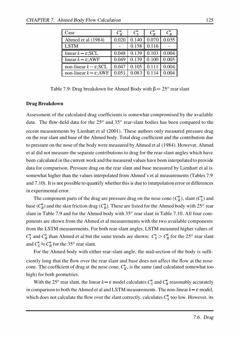
7/17/2019 Big
http://slidepdf.com/reader/full/big563db8d5550346aa9a975e13 142/189
CHAPTER 7. Ahmed Body Flow Calculation 125
Case C K C
S C B C
R
Ahmed et al (1984) 0.020 0.140 0.070 0.055
LSTM - 0.158 0.116 -
linear k ε;SCL 0.048 0.139 0.103 0.004
linear k ε;AWF 0.049 0.139 0 .100 0 .005
non-linear k ε;SCL 0.047 0.105 0.111 0.004
non-linear k ε;AWF 0.051 0.083 0.114 0.004
Table 7.9: Drag breakdown for Ahmed Body with β 25o rear slant
Drag Breakdown
Assessment of the calculated drag coefficients is somewhat compromised by the available
data. The flow-field data for the 25o and 35o rear-slant bodies has been compared to the
recent measurements by Lienhart et al (2001). These authors only measured pressure drag
on the rear slant and base of the Ahmed body. Total drag coefficient and the contribution due
to pressure on the nose of the body were measured by Ahmed et al (1984). However, Ahmed
et al did not measure the separate contributions to drag for the rear-slant angles which have
been calculated in the current work and the measured values have been interpolated to provide
data for comparison. Pressure drag on the rear slant and base measured by Lienhart et al is
somewhat higher than the values interpolated from Ahmed’s et al measurements (Tables 7.9
and 7.10). It is not possible to quantify whether this is due to interpolation error or differences
in experimental error.
The component parts of the drag are pressure drag on the nose cone (C K ), slant (C
S ) and
base (C B) and the skin friction drag (C
R). These are listed for the Ahmed body with 25o rear
slant in Table 7.9 and for the Ahmed body with 35o rear slant in Table 7.10. All four com-
ponents are shown from the Ahmed et al measurements with the two available components
from the LSTM measurements. For both rear-slant angles, LSTM measured higher values of
C S and C
B than Ahmed et al but the same trends are shown: C S
C B for the 25o rear slant
and C S
C B for the 35o rear slant.
For the Ahmed body with either rear-slant angle, the mid-section of the body is suffi-
ciently long that the flow over the rear slant and base does not affect the flow at the nose
cone. The coefficient of drag at the nose cone, C K , is the same (and calculated somewhat too
high) for both geometries.
With the 25o rear slant, the linear k ε model calculates C S and C B reasonably accurately
in comparison to both the Ahmed et al and LSTM measurements. The non-linear k ε model,
which does not calculate the flow over the slant correctly, calculates C S too low. However, its
7.6. Drag

7/17/2019 Big
http://slidepdf.com/reader/full/big563db8d5550346aa9a975e13 143/189
CHAPTER 7. Ahmed Body Flow Calculation 126
Case C K C
S C B C
R
Ahmed et al (1984) 0.020 0.095 0.090 0.055
LSTM - 0.121 0.129 -
linear k ε;SCL 0.046 0.134 0.102 0.004
linear k ε;AWF 0.047 0.112 0 .103 0 .005
non-linear k ε;SCL 0.047 0.088 0.093 0.004
non-linear k ε;AWF 0.052 0.088 0.099 0.004
Table 7.10: Drag breakdown for Ahmed Body with β 35o rear slant
calculation of the base pressure-drag coefficient, C B, is accurate in comparison to the LSTM
measured value. (The flow is fully separated behind the base when calculated by either the
linear or non-linear model.)
When using the SCL wall function with the non-linear k ε model, the UMIST convec-
tion scheme was used to calculate both the mean velocity and turbulence variables; the model
with AWF wall function used the UPWIND scheme for turbulence variables (Table 7.1). The
difference in a accuracy of these schemes is partly the cause of the improved calculation of
C S when using the SCL wall function.
Although they show quite different magnitudes, both sets of measurements show C S
C B
for the 35o rear-slant geometry. All the calculations (except linear k ε with SCL) show this,
but as the calculations with the linear model agree better with the LSTM measurements and
the calculations with the non-linear model agree better with the Ahmed et al measurements,
it is hard to draw further conclusions.
Skin friction drag, C R, is principally generated on the mid-section of the body and is
approximately the same for both rear-slant angles. However, it is calculated significantly
too low - by an order of magnitude - for both geometries and an assessment of the accuracy
of Ahmed et al’s calculation of C R is required. Ahmed et al used a strain-gauge balance to
measure the total coefficient of drag (C W ) and calculated C K
C S and C
B by integrating the
measured pressure over the relevant surfaces. The skin friction drag coefficient was then
calculated by:
C
R
C W
C
K
C
S
C
B
(7.7)
Clearly, any inaccuracy in the total drag measurement or calculation of the pressure drag
components will be absorbed into C R. Taking the β
25o geometry as an example, the
values of C S and C
B calculated from LSTM’s measurements (Table 7.9) are somewhat larger
than those calculated by Ahmed et al. If these values are substituted into Equation 7.7 then
assuming that Ahmed et al’s measurement of C W is accurate, C K
C R 0 011 This is half
7.6. Drag

7/17/2019 Big
http://slidepdf.com/reader/full/big563db8d5550346aa9a975e13 144/189
CHAPTER 7. Ahmed Body Flow Calculation 127
the value of the measured C K alone and emphasises the incompatibility between the two sets
of measurements. The calculated values of C R shown in Tables 7.9 and 7.10 may indeed be
the correct order of magnitude, but more detailed measurements would be required to prove
this.
7.7 Conclusions
The results presented in this chapter have shown that the flow around the Ahmed body can be
calculated to a reasonable degree of accuracy using the RANS equations and two-equation
turbulence models. Both the attached flow with strong vortices (25o rear slant) and fully
separated flow (35o rear slant) can be calculated. Moreover, the calculation of the body’s
drag with the 35o rear-slant angle using the non-linear k ε model and AWF wall function
is sufficiently accurate for industrial purposes (in comparison to Ahmed’s et al, 1984, data).However, the calculation of the flow over the body with the 25 o rear slant is not sufficiently
accurate. Furthermore, the current formulation of the non-linear k ε model is not appropri-
ate for calculating the flow over the body with 25o rear-slant angle.
There are a number of specific conclusions which can be drawn from the calculation of
the Ahmed body flow and which are addressed separately.
Boundary Layers on Body Mid-Section The boundary layers calculated on the mid-
section of the body are thicker than the measured boundary layers. This makes the flow
more susceptible to separation in an adverse pressure gradient such as over the rear slant.
The thickening of the boundary layers is most probably due to the use of large near-wall cells
in which 100
y
200. Also in this region, the calculated outer flow is accelerated due to
the blockage effect of the body and the use of symmetry planes at the domain boundary. If
further calculations are to be made on the Ahmed body, an investigation of the effect of reduc-
ing y should be made and the domain boundary condition altered to prevent the acceleration
of the outer flow.
Side-Edge Vortex Formation Flow in a 25o expansion would normally be expected to
separate from the walls due to the adverse pressure gradient encountered. However, mea-
surements by Ahmed et al (1984) and Lienhart et al (2001) show that flow over the Ahmed
body with a 25o rear slant remains attached. Strong longitudinal vortices are formed at the
side edges of the slant, which draw fluid out of the boundary layer on the slant and cause the
flow to remain attached. The linear k ε model calculates a vortex which is strong enough
to retain the attached flow. The non-linear model calculates a weaker vortex. When using
7.7. Conclusions

7/17/2019 Big
http://slidepdf.com/reader/full/big563db8d5550346aa9a975e13 145/189
CHAPTER 7. Ahmed Body Flow Calculation 128
a first-order convection scheme (UPWIND), this vortex is sufficiently diffuse to affect the
whole rear slant and produce attached flow. When using a higher-order convection scheme
(UMIST), the vortex is confined to a smaller region. It does not draw fluid out of the boundary
layer over a sufficiently large region of the slant to prevent separation.
Components of Non-linear Model The weak side-edge vortex calculated on the 25o rear
slant by the non-linear model was caused by the mean strain bending being calculated too low
in the region of the side edge. It was not possible to identify the specific feature of the non-
linear model which caused this, as both the functional form of c µ and the inclusion of non-
linear components in the Reynolds stresses was sufficient to cause separated flow. Craft et al
(1996b) tuned the coefficients of the non-linear model by testing the model in homogeneous
shear flow, fully developed swirling flow and flow with streamline curvature. In this case,
however, the flow is characterised by streamwise vorticity and an adverse pressure gradient.
The calculation of streamwise vorticity is influenced by the Reynolds normal and shear stress
generation (the 3rd and 4th terms of the right-hand side of Equation 7.5). These terms are zero
in the linear calculation but may well be significant in the non-linear k ε model calculation7.
It is therefore possible, that the model coefficients need re-tuning if it is to be used to calculate
flow in an adverse pressure gradient (or separated flow) with streamwise vorticity.
Similarly, it is possible that the functional form of c µ causes too great a reduction in
turbulent viscosity over the rear slant. (The c µ function is defined from measurements and
DNS calculations in homogeneous shear flow). With the thickened boundary layer over the
top surface of the body, the flow is susceptible to separation in adverse pressure gradients.The combined effect of low turbulent viscosity and a thick boundary layer then cause flow
separation, which inhibits the side-edge vortex formation.
Effect of Realizability in the Linear Calculation The realizability condition, which re-
duces turbulent viscosity in regions of high strain rate, was used in the calculations with the
linear k ε model. In comparison to the linear model without the condition, it significantly
improved the calculation of mean velocity and length of the recirculating flow region in the
wake of the body with 35o rear slant.
Calculation of Drag and Influence of Wall Function The calculation of drag induced
by flow over the body with the 25o rear slant is reasonable, but not sufficiently accurate
for industrial purposes. Although calculations for this case with the linear model produce
attached flow over the slant, the base pressure and overall drag are too high in comparison to
7There is insufficient measured data in the relevant areas around the slant to prove this conclusively.
7.7. Conclusions
7/17/2019 Big
http://slidepdf.com/reader/full/big563db8d5550346aa9a975e13 146/189
CHAPTER 7. Ahmed Body Flow Calculation 129
Ahmed’s et al (1984) measurement. The non-linear model calculates separated flow over the
rear slant and the distribution of drag between the rear slant and base is poor.
Both the linear and non-linear model calculate separated flow over the 35o rear slant. Drag
calculated by the linear model is too high for this case but drag calculated by the non-linear
model is much more accurate. Indeed, when the non-linear model is used with the AWF wallfunction, the calculated drag is sufficiently accurate for industrial use.
In all the cases where the correct flow profile is calculated, use of the AWF wall function
improves the calculation of drag in comparison to the SCL wall function. In all the calcu-
lations, the component of drag due to friction is an order of magnitude lower than the value
given by Ahmed et al. (It should be noted that Ahmed et al did not measure friction drag
directly, but calculated it from the difference between the total drag and the pressure drag.
Consequently, any errors in the measured pressure and total drag are passed on to the friction
drag.)
7.7. Conclusions

7/17/2019 Big
http://slidepdf.com/reader/full/big563db8d5550346aa9a975e13 147/189
Chapter 8
Conclusions and Recommendations for
Future Work
8.1 Preliminary Remarks
The aim of the work presented in this thesis has been to test the cubic non-linear k ε model
of Craft et al (1996b) in a number of flows pertinent to road vehicle aerodynamics. These are
flows which contain features such as separation, streamline curvature, streamwise vorticity
and vortex shedding. A secondary aim has been to test the suitability of a newly developed
analytical wall function. The non-linear turbulence model was tested in three flows with
simple geometries which had at least some of the flow complexity found in the flow around
road vehicles. In these computations, the non-linear model was shown on the whole to be
more accurate than a linear k ε model. The final test case, the flow around a simplified
model of a car was calculated with both linear and non-linear k ε models.
Conclusions have already been presented on a case-by-case basis at the end of each of
the flow calculation Chapters. It is not intended to repeat those conclusions here, but to
re-emphasise the salient points and to make recommendations for future work.
8.2 Conclusions
Flow Around a Cylinder of Square Cross Section Close to a Wall
In the flow with the steady wake
g
d 0 25 , velocity profiles calculated in the wake
of the cylinder by the non-linear k ε model are not so accurate as those calculated
by the linear model. In contrast, Reynolds stresses are calculated more accurately by
the non-linear k ε model than the linear model. The linear model is very sensitive
131

7/17/2019 Big
http://slidepdf.com/reader/full/big563db8d5550346aa9a975e13 148/189
CHAPTER 8. Conclusions and Recommendations for Future Work 132
to changes in the upstream value of turbulence dissipation rate specified at the inlet,
whereas the non-linear model is not. In a flow which is similarly insensitive to changes
in inlet turbulence intensity, this insensitivity is a desirable feature of the non-linear
model. It is often the case in industrial calculations that the inlet values of turbulence
are not known.
When the cylinder is placed sufficiently far from the wall that periodic vortex-shedding
occurs
g
d 0
50and0
75 , the non-linear k ε model calculates the frequency of
the vortex-shedding more accurately than the linear model. The non-linear model
calculates the time-averaged total stresses in the wake
ut iut
j
too high. Moreover,
the relative magnitudes of the contributions to total stress are the wrong way round:
the time-averaged periodic motion stresses ui u j
are too high and the time-averaged
Reynolds stresses
uiu j
are too low.
Flow in a U-bend of Square Cross Section
The non-linear k ε model is virtually as accurate as a cubic DSM in calculating the
mean velocities and complex secondary flow pattern in this flow with strong streamline
curvature and streamwise vorticity.
The non-linear k ε model calculates the Reynolds stresses reasonably well but is
not so accurate as the cubic DSM. In this flow, transport of the Reynolds stresses is
significant; the non-linear k ε model does not accurately account for Reynolds stress
transport.
Flow in a 10o Plane Diffuser
The non-linear k ε model calculates the mean velocities and Reynolds stresses signif-
icantly better than the linear model. Indeed when a log-law wall function is used, the
non-linear model correctly calculates flow separation on the inclined wall of the dif-
fuser whereas the linear model does not. However, the magnitude of the flow reversal
calculated by the non-linear model is not as great as that measured.
The ability of the non-linear k ε model to calculate the velocity more accurately than
the linear model in a separated flow is contrary to the findings of the square cross-
sectioned cylinder close to a wall (steady flow) test case. The difference between the
two cases is that in the plane diffuser, the adverse pressure gradient is relatively weak
and the non-linear model is the more sensitive to this. In the wake of the square cross-
sectioned cylinder the adverse pressure gradient is much stronger and there are other
8.2. Conclusions

7/17/2019 Big
http://slidepdf.com/reader/full/big563db8d5550346aa9a975e13 149/189
CHAPTER 8. Conclusions and Recommendations for Future Work 133
effects influencing the flow calculation, such as impingement at the leading face and
stronger curvature of the streamlines.
Flow Around the Ahmed Body
For the Ahmed body with the 25o rear slant the non-linear k ε model does not calcu-
late the flow over the slant correctly. It calculates separated, rather than attached flow
over the majority of the slant. In contrast, the linear model does calculate attached flow
over the whole slant but is not able to calculate the initial separation at the leading edge
of the slant.
The failure of the non-linear k ε model to calculate attached flow on the slant is
principally due to its failure to calculate a sufficiently strong side-edge vortex. This
is somewhat surprising as the non-linear model is well able to calculate flows with
streamwise vorticity, as is shown by the swirling-flow tests of Suga’s (1995) original
study of this turbulence model and by the square cross-sectioned U-bend test case in
the present study. It should be noted that unlike flow around the Ahmed body, the U-
bend is an enclosed flow and influenced by the strong radial pressure gradient. In light
of the findings of the current work, this may well have a bearing on the performance of
the non-linear model.
For the Ahmed body with the 35o slant both the non-linear and linear k ε models
calculate the correct, separated flow over the rear slant. In common with the square
cross-sectioned cylinder case, the velocity profiles in the wake are calculated more
accurately by the linear model. However, the non-linear model calculates drag on the
Ahmed body more accurately than the linear model. When used in conjunction with
the analytical wall function, the non-linear model calculates the drag on the body to the
degree of accuracy required by industry.
Analytical Wall Function
Calculations of the 10o plane diffuser flow with the AWF show that this wall function
calculates near-wall effects more accurately than a log-law type wall function (SCL).When used with the the linear k ε model, the AWF improves the flow calculation
to the extent that a small amount of separation is calculated (whereas separation is
not calculated with an SCL wall function). When used with the non-linear model, the
AWF improves the calculation of the separated flow. Of the models tested in this work,
the combination of the non-linear k ε model and AWF provides the most accurate
calculation for this case.
8.2. Conclusions

7/17/2019 Big
http://slidepdf.com/reader/full/big563db8d5550346aa9a975e13 150/189
CHAPTER 8. Conclusions and Recommendations for Future Work 134
Calculations of the flow around the Ahmed body with the AWF show that when the
correct mode of flow is calculated1 the AWF improves the calculation of drag. No
significant changes in the mean velocity profiles are apparent when using the AWF
rather than the SCL wall function. As with the plane diffuser, the non-linear k ε
model and AWF provide the most accurate combination of the models tested. It shouldbe noted that the distance from the wall of the near-wall nodes used in the Ahmed body
calculations was relatively large. This reduces the potential for the AWF to improve
the calculation and it would be reasonable to expect the AWF to improve further the
near-wall flow if the near-wall cell size were refined.
Realizability Condition
The realizability condition was initially introduced to the Ahmed body flow calcula-
tions as a mathematically nicety; it prevents the spurious growth of turbulent viscosityin regions of low turbulence intensity and improves the stability of the calculations.
However, it has also been shown that the use of the realizability condition improves the
calculation of the wake-velocity profiles.
8.3 Recommendations for Future Work
Ahmed Body Calculations
Future calculations of the Ahmed body flow should include a grid refinement study.
In particular, a sensitivity study of the distance to the body of the near-wall nodes
should be made. This will show whether the boundary layers around the body can be
calculated more accurately than in the present study and help to determine whether
thickening of the boundary layers is a cause of the excessive flow separation calculated
by the non-linear k ε model. It will also help to determine the influence of the near-
wall skewing of velocity over the rear slant.
The current work uses symmetry planes to represent the open boundaries of the wind
tunnel which leads to an acceleration of the flow around the body that is not measured.
Future calculations should modify this boundary condition to an “entrainment” type
boundary or expand the grid in the region of the cylinder to prevent the calculation of
the favourable pressure gradient which accelerates the flow.
1ie. when the linear k ε model is used to calculate the flow around the body with the 25o rear slant or when
either the linear or non-linear model is used to calculate the flow around the body with the 35 o rear slant
8.3. Recommendations for Future Work
7/17/2019 Big
http://slidepdf.com/reader/full/big563db8d5550346aa9a975e13 151/189
CHAPTER 8. Conclusions and Recommendations for Future Work 135
Non-linear k ε Model
As the non-linear k ε model appears not to be able to calculate sufficient streamwise
vorticity in a free-stream flow, a simple test case should be sought to study this feature.
The coefficients in the stress-strain relationship of the non-linear k
ε model were not
originally tuned for separated flows. As the current work shows conflicting results for
the accuracy of the non-linear model in relatively weak and strong adverse pressure
gradients, future development of the non-linear model should attempt to define which
elements of the model need to be re-cast to provide consistent performance in sepa-
rated flows. In particular, the relevant influence of the c µ function and the non-linear
contribution to the Reynolds stresses should be studied in separated flow. Either of
these features in isolation in the non-linear model are sufficient to cause separation of
the flow over the 25o rear-slant Ahmed body.
Further study should be made of the non-linear k ε model’s ability to calculate pe-
riodic flows. Such a study would aim to establish why the time-averaged Reynolds
stresses are calculated too low and the time-averaged periodic motion stresses are too
high in the wake of the square cylinder .
Analytical Wall Function
The current form of the analytical wall function is based on the solution of a simplified
momentum equation in the near-wall cell which does not include non-linear contribu-
tions to the Reynolds stresses. For consistency, when the analytical wall function is
used with the non-linear k ε model, it should be be re-cast to include contributions of
the non-linear stresses to the simplified momentum equation.
Stability enhancing measures should be sought for the analytical wall function to miti-
gate the effect of placing the momentum source in the constant (S C ) rather than coeffi-
cient
S P) part of the linearised source term.
8.3. Recommendations for Future Work
7/17/2019 Big
http://slidepdf.com/reader/full/big563db8d5550346aa9a975e13 152/189
Appendix A
Realizability Condition for an EVM
A.1 Introduction
The realizability conditions by which the Reynolds stresses are constrained are:
uiu j 0 ; i
j (A.1)
uiu j2
uiui
u ju j (A.2)
det
uiu j
0 (A.3)
Schumann (1977) discusses these conditions and some of their consequences for turbulence
modelling; Lumley (1978) discusses their application to Differential Stress Models in greater
detail. The realizability conditions are more readily applied in a DSM than an EVM as
transport equations are solved for the various turbulent stresses and limiting values can be
applied. In an EVM the turbulent stresses are not calculated explicitly, but turbulent viscosity
is calculated from the turbulent kinetic energy, k and dissipation rate, ε If these are not
controlled in an EVM flow calculation, it is possible that negative values of k and ε may
occur leading to numerical instability. By setting a lower limit for k (eg k 10
30), negative
values can be avoided without any detrimental numerical problems. A more sophisticated
approach is necessary for ε. In a k ε EVM the turbulent viscosity depends on the reciprocal
of ε : µt ρc µ
k 2
ε (A.4)
Thus very small values of ε may create erroneously large values of µ t . A simple method of
controlling ε would be to set its lower limit to an arbitrarily low value such as: εmin 10
20εo
(where εo is the inlet or far-field value); this can still lead to unacceptably high levels in µ t .
Moore & Moore (1999) conducted a review of methods used to control excessive levels of
137
7/17/2019 Big
http://slidepdf.com/reader/full/big563db8d5550346aa9a975e13 153/189
APPENDIX A. Realizability Condition for an EVM 138
µt . These use a functional form of c µ which decreases its value in regions of flow with high
strain rates, controlling the growth of µt . These functional forms of c µ are generally formu-
lated without reference to the concept of realizability. May (1998) reworked the realizability
conditions for an EVM to obtain a method by which µt could be limited. This Appendix de-
scribes how the realizability condition can be defined for an EVM. Throughout the derivation,the summation convention for terms containing repeated indices is not applied.
A.2 Mathematical Formulation
If one takes the Schwarz inequalities (Equation A.1 & A.2) and uses the eddy-viscosity hy-
pothesis for a linear EVM:
ρu
iu
j
2
3 ρδi jk
µ
t
∂U i
∂ x j
∂U j
∂ xi
(A.5)
then for the case i 1; j
2 the Reynolds stress components may be written:
ρuv
2
µ2t A2 (A.6)
ρuu
µt B C
0 (A.7)
ρvv
µt D C
0 (A.8)
and the terms A
B
C
D are:
A
∂U
∂ y
∂V
∂ x
(A.9)
B
2∂U
∂ x (A.10)
C
2
3ρk (A.11)
D
2∂V
∂ y(A.12)
Substituting Equation A.6-A.8 into the Schwarz inequality (Equation A.2):
A2 µ2t
Bµt C
Dµt C (A.13)
This can be re-written as:
C µt α
C µt β
0 (A.14)
where:
A.2. Mathematical Formulation

7/17/2019 Big
http://slidepdf.com/reader/full/big563db8d5550346aa9a975e13 154/189
APPENDIX A. Realizability Condition for an EVM 139
α
1
2
B D
B D 2
4 A2
1 2
β
1
2
B D
B D 2 4 A2
1 2
(A.15)
To satisfy the inequality in Equation A.14, there are two cases which need to be considered.
Case 1:
C µt α ; C
µt β (A.16)
and Case 2:
C µt α ; C
µt β (A.17)
Substitution of β from Equation A.15 into the second part of the Case 2 condition (Equation
A.17) gives:
2C
µt
B
D
µt
B D
2
4 A2
1 2(A.18)
and summing the inequalities given with the normal stresses in Equations A.7 and A.8, gives:
2C µt
B D
0 (A.19)
Now Equation A.19 determines that the left hand side of Equation A.18 must be positive.
If both sides of Equation A.18 are multiplied by
1 then the inequality reverses and this
equation states that the square root of the term in square brackets must be less than or equal
to zero. This is not possible for non-zero, real numbers and hence Case 2 (Equation A.17)
cannot be true for any value but zero. For Case 1, the first inequality of Equation A.16
includes the second inequality and hence the only condition which must be satisfied is:
C
µt α (A.20)
Replacing C
µt α with their respective values from Eqns.A.11, A.4 and A.19, gives:
ε 34
c µk
B D
B D
2 4 A2
1 2
This and similar analyses for the cases: i 1; j
3 and i
2; j
3 provide three criteria for
the minimum value of ε:
ε1
3
2c µk
∂U
∂ x
∂V
∂ y
∂V
∂ y
∂U
∂ x
2
∂U
∂ y
∂V
∂ x
2
1 2
(A.21)
A.2. Mathematical Formulation
7/17/2019 Big
http://slidepdf.com/reader/full/big563db8d5550346aa9a975e13 155/189
APPENDIX A. Realizability Condition for an EVM 140
ε2
3
2c µk
∂V
∂ y
∂W
∂ z
∂W
∂ z
∂V
∂ y
2
∂V
∂ z
∂W
∂ y
2
1 2
(A.22)
ε3
3
2c µk
∂W
∂ z
∂U
∂ x
∂U
∂ x
∂W
∂ z
2
∂W
∂ x
∂U
∂ z
2
1 2
(A.23)
A.3 Implementation in STREAM
The realizability condition has been implemented in STREAM immediately after µt has been
updated from the newly calculated values of k and ε by applying the criterion:
µt min
µt
ρk
max
TINY α1
α2 α3
(A.24)
where T INY is an arbitrarily small value and α1 α2 α3 are derived from Equation A.15 and
take the values from the outer set of parentheses in Equations A.21 to A.23 as follows:
α1
3
2
∂U
∂ x
∂V
∂ y
∂V
∂ y
∂U
∂ x
2
∂U
∂ y
∂V
∂ x
2
1 2
(A.25)
α2
3
2
∂V
∂ y
∂W
∂ z
∂W
∂ z
∂V
∂ y
2
∂V
∂ z
∂W
∂ y
2
1 2
(A.26)
α3
3
2
∂W
∂ z
∂U
∂ x
∂U
∂ x
∂W
∂ z
2
∂W
∂ x
∂U
∂ z
2
1 2
(A.27)
A.4 Comparison with c µ Function
The realizability condition described in this Appendix acts in a similar way to the functional
forms of c µ described in Equations 2.28 and 2.32: both act to reduce the turbulent viscosity
in regions of high velocity gradient. Indeed the realizability condition can be re-cast as a
functional form of c µ. If one considers a homogeneous simple shear where the only velocity
gradient is ∂U
∂ y and taking the latter part of the minimum function in Equation A.24:
µt
2
3
ρk
∂U
∂ y(A.28)
A.3. Implementation in STREAM
7/17/2019 Big
http://slidepdf.com/reader/full/big563db8d5550346aa9a975e13 156/189
APPENDIX A. Realizability Condition for an EVM 141
From Equation 2.29, in a simple shear ∂U
∂ y
S ε
k , and using Equation A.4 for the turbulent
viscosity:
c µρk 2
ε
2
3
ρk
S ε
k (A.29)
which provides the following function for c µ:
c µ
2
3S (A.30)
The performance of this new c µ compared with the original versions (Equations 2.28 and
2.32) is shown in Figure 2.1. It is apparent that the effective c µ defined by the realizability
condition is not reduced in the presence of high strain rates as much as the other forms.
A.4. Comparison with c µ Function

7/17/2019 Big
http://slidepdf.com/reader/full/big563db8d5550346aa9a975e13 157/189
Appendix B
Derivation of the Analytical Wall
Function
B.1 Specification of Analytical Wall Function
B.1.1 Dimensionless Simplified Momentum Equation
A simplified momentum equation can be written for the near-wall region as follows:
ρ∂UU
∂ x ρ
∂UV
∂ y
∂P
∂ x
∂
∂ y
µ µt
∂U
∂ y
(B.1)
where ρ
µ
µt
P are the density, laminar viscosity, turbulent viscosity and pressure respec-tively, U and V are the mean velocity of the flow tangential and normal to the wall respec-
tively, x and y are the coordinates tangential and normal to the wall respectively (not nec-
essarily the Cartesian directions). This momentum equation retains the simple shear flow
assumption that diffusion in the x-direction (tangential to the wall) is negligible compared
to diffusion in the y-direction (normal to the wall). In a fully developed flow, convection
of momentum tangential to the wall is zero as there is no gradient in the tangential velocity
(∂U
∂ x) - this is not the case for developing flows. Inclusion of convection normal to the
wall is important when considering separation and reattachment of the flow where there are
significant velocities towards and away from the wall.
The simplified momentum equation is converted to a dimensionless form by application
of the reference velocity
U re f , distance
d re f and density
ρre f . These are the values which
are used to detemine the Reynolds number of the flow and their application provides dimen-
sionless velocities
U
V
, distances
x , y
, density
ρ
, viscosity
µ
and pressure
P
.
The version of the STREAM code into which this model is incorporated is non-dimensional,
142
7/17/2019 Big
http://slidepdf.com/reader/full/big563db8d5550346aa9a975e13 158/189
APPENDIX B. Derivation of the Analytical Wall Function 143
and hence it is convenient to express this model in non-dimensional variables which are de-
noted by a prime.
U
U
U re f ; V
V
U re f ; (B.2)
Substituting these into Equation B.1 and reworking, gives the following form of the momen-
tum equation:
U
∂U
∂ x
V
∂U
∂ y
∂P
∂ x
∂
∂ y
µ
µ t
∂U
∂ y
(B.3)
A code-specific simplification has been used here. The incompressible, non-dimensional
version of STREAM sets the density as: ρ ρ
ρre f
1 0. This has been used to simplify
Equation B.3.
B.1.2 Analytical Solution of Equations
When considering the near-wall effects it is more appropriate to use a wall-distance scaled
by the near-wall properties ( y
), rather than the bulk flow conditions ( y ). Hence, the wall
distance is substituted and the terms of Equation B.3 are re-arranged:
y
yk 1 2
ν
y k
1 2 p
ν
∂
∂ y
1
µt
µ
∂U
∂ y
ν
k p
∂P
∂ x
U
∂U
∂ x
V
∂U
∂ y
C (B.4)
C is a constant, ν
ν
d re f U re f is the non-dimensional kinematic viscosity and k
p is the
non-dimensional turbulent kinetic energy at the near-wall node p (Figure 2.3). It is assumed
that k varies quadratically in the viscous sublayer and remains constant in the fully turbulent
region. (This is the same assumption that is used in the simplified version of the Chieng &
Launder, 1980, wall function.)
A more sophisticated approach would be to use k
v - ie the value of turbulent kinetic energyat the edge of the viscous sublayer. This is the value used in the full Chieng & Launder (1980)
wall function which makes the value of τ w less dependent on the size of the near-wall cell and
the location of the near-wall node. k v is calculated by assuming a linear profile for k
in the
fully turbulent region, a constant sublayer Reynolds number, k
1 2
v y v
ν
20 and extrapolating
a value from the two near-wall nodes, p and N . Johnson & Launder (1982) used a similar
B.1. Specification of Analytical Wall Function

7/17/2019 Big
http://slidepdf.com/reader/full/big563db8d5550346aa9a975e13 159/189
APPENDIX B. Derivation of the Analytical Wall Function 144
technique but allow variation in the sublayer thickness:
R v
k 1
2
v yv
ν
20
1 3 1λ λ
k v
k w
k v
(B.5)
where k
w is the wall value of turbulent kinetic energy and k
v and k
w are extrapolated fromnodes p and N . The extrapolation of k
v and k w can cause problems. There is a maximum in
the turbulent kinetic energy profile near to the wall and depending on resolution of the grid,
the relative positions of nodes p and N may result in greatly differing values of k w and k
v
(Figure 2.4). The value of k p is also sensitive to the position of node p. However, by using
constant k k
p in the near-wall cell the additional uncertainty of extrapolating values for k v
and k w is removed. This is considered a more robust practice to adopt during the development
of the new wall function.
Solution Within the Viscous Sub-layer
In the viscous sublayer (referred to herein as Region 1) the flow is laminar and the following
conditions are specified:
y
y v ; µ t 0 (B.6)
where yv is the non-dimensional thickness of the viscous sub-layer in wall units. Equation
B.4 is then reduced to:
∂
∂ y
∂U
1
∂ y
C 1 (B.7)
∂U
1
∂ y
C 1 y
A1 (B.8)
U
1
C 1 y
2
2
A1 y
B1 (B.9)
where the subscript on U 1, A1
B1 and C 1 denotes Region 1: the viscous sub-layer. At the wall
the following boundary conditions apply: y
0, U
1 0 hence, B1 0, and:
U
1
C 1 y
2
2
A1 y (B.10)
Solution Outside the Viscous Sub-layer
Outside the viscous sub-layer in the fully turbulent region (Region 2) an analytical solution
is again sought for Equation B.4. The turbulent viscosity, µt must be retained in this region
B.1. Specification of Analytical Wall Function

7/17/2019 Big
http://slidepdf.com/reader/full/big563db8d5550346aa9a975e13 160/189
APPENDIX B. Derivation of the Analytical Wall Function 145
and it is specified from the Prandtl-Kolmogorov condition, µt ρc µk 1 2l. As this is to be
applied in the near-wall region the turbulent length scale, l , is specified as; l
cl
y yv and
the turbulent kinetic energy is given the near-wall cell-centre value, k p Writing µt in terms
of the wall distance, y gives:
µt ρk
1 2
p α
y
y v
ν
k 1
2
p
(B.11)
which reduces to the following non-dimensional form:
µ t µ α
y
y v (B.12)
where α c µcl and the constants c µ and cl take the values 0.09 and 2.55 respectively. In the
fully turbulent region, Equation B.4 now becomes:
∂
∂ y
1 α
y
y v
∂U
2
∂ y
C 2 (B.13)
which can be integrated to find U
2 :
∂U
2
∂ y
C 2 y
1 α
y
yv
A2
1 α
y
yv
(B.14)
U
2 C 2
y
1 α
y
yv
dy
A2
dy
1 α
y
yv
(B.15)
U
2
C 2 y
α
A2
α
C 2
α y ν
1
α2
ln
1 α
y
y v
D2 (B.16)
(Note: the subscript “2” denotes the region outside the viscous sub-layer.) Boundary condi-
tions can be set at the edge of the viscous sub-layer:
y
y v ; U
1
U
2 ;∂U
1
∂ y
∂U
2
∂ y
(B.17)
Applying the boundary conditions to Equation B.14 gives:
A2 A1
y v
C 1 C 2 (B.18)
and to Equation B.16 gives:
D2
C 1 y
2v
2
A1
C 2
α
y v (B.19)
B.1. Specification of Analytical Wall Function
7/17/2019 Big
http://slidepdf.com/reader/full/big563db8d5550346aa9a975e13 161/189
APPENDIX B. Derivation of the Analytical Wall Function 146
and the velocity in the fully turbulent region may now be written as:
U
2
C 2
α
y
y v
A1
α
C 1 y ν
α
C 2
α2
ln
1 α
y
y v
C 1 y
2v
2
A1 y v (B.20)
It is necessary to set one further boundary condition for the fully turbulent flow region at the
near-wall cell face opposite the wall:
y
y n ; U
2 U n (B.21)
U n is the resultant velocity in the direction of flow along the wall, located at the cell face
between the near-wall cell and the adjacent cell on the flow side of the domain. In a cell-
centred code, this must be found by interpolation of the resultant velocities at the centres of
the near-wall cell and the adjacent cell. By applying these conditions to Equation B.20 andrearranging, an expression for the integration constant A1 can be recovered:
A1
αU n
C 2
yn
yv
C 1 y v
C 2α
ln
1 α
yn
yv
αC 1 y
2v
2
α yv ln
1 α
yn
yv
(B.22)
B.1.3 Specification of Wall Shear Stress, τ w
A non-dimensional shear stress can be defined as:
τ w
µ
∂U
∂ y
(B.23)
and can be written in terms of the wall distance, y :
τ w
k 1
2
p
ρre f
∂U
∂ y
(B.24)
At the wall (ie within the viscous sub-layer), the wall distance y
0 and the velocity gradient
is specified by Equation B.8. The wall shear stress can now be defined:
τ w
k 1
2 p
ρre f
A1 (B.25)
B.1.4 Average Production of Turbulent Kinetic Energy, Pk
The average value of production of turbulent kinetic energy in the near-wall cell can be spec-
ified in non-dimensional units as:
B.1. Specification of Analytical Wall Function

7/17/2019 Big
http://slidepdf.com/reader/full/big563db8d5550346aa9a975e13 162/189
APPENDIX B. Derivation of the Analytical Wall Function 147
Pk
1
yn
y
n
y
v
ρ uv
∂U
2
∂ y
dy
1
yn
yn
yv
ρuv
∂U
2
∂ y
dy (B.26)
The velocity gradient is given by Equations B.14 & B.18, and the integral can thus be written:
Pk
ρ y
n
y n
yv
uv
A1 C 1 y v C 2
y
y v
1 α
y
yv
dy (B.27)
The shear stress is defined from the eddy viscosity hypothesis:
uv νt
dU
dy (B.28)
Recasting in dimensionless terms:
uv
ν t
dU
dy
ν t
dU
dy
k 1
2
p
ν
(B.29)
and substituting Equation B.12 for νt
ν :
uv
α
y
y v
dU
dy
k 1
2
p (B.30)
In the fully turbulent region the velocity gradient is given by Equation B.14, resulting in the
final expression for shear stress:
uv
k 1
2 p α
y
y v
A1
C 1 y
v
C 2
y
y
v
1 α
y
yv
(B.31)
The production of turbulent kinetic energy can now be defined as:
Pk
ραk 1
2
p
yn
yn
yv
y
y v
A1
C 1 y v
C 2
y
yv
1 α
y
yv
2
dy (B.32)
This can either be calculated numerically, within the CFD scheme, or by the analytical solu-
tion:
Pk
ρk 1 2
p
α yn
y n y v
C 22
2α2
2 α
y n y v
C 2
2 A1 2C 1 y v
3C 2
α
A1 C 1 y v
C 2
α
A1 C 1 y v
3C 2
4
ln
1 α
y n y v
(B.33)
B.1. Specification of Analytical Wall Function

7/17/2019 Big
http://slidepdf.com/reader/full/big563db8d5550346aa9a975e13 163/189
APPENDIX B. Derivation of the Analytical Wall Function 148
α
yn
yv
A1 C 1 y v
C 2α
2
1 α
yn
yv
B.1.5 Average Turbulence Dissipation Rate, ε
The average dissipation rate specified in the near-wall cell used with the analytical wall func-
tion is a simplified version of the term proposed by Chieng and Launder (1980). This is
derived from the assumption that close to the wall, in the viscous wall layer, the dissipation
is constant and equal to its wall limiting value given by: ( y yε)
ε
1 2 ν
∂k
1 2
∂ y
2
2 ν k
p
y
2ε
(B.34)
In the Chieng & Launder scheme the height of the dissipation sub-layer is taken to be: yε
yv.Further away from the wall, in the fully turbulent flow region, dissipation rate is given by:
( y
yε)
ε
2
k 3 2
p
cl y
(B.35)
Integrating these two values over their respective sections of the near-wall cell and summing
gives the average dissipation rate:
ε
1 y
n
y
ε
0
2 ν
k
p
y
2ε
dy
y
n
y
ε
k
3 2
pcl y
dy
1 y
n
2 ν
k
p y
ε k
3 2
pcl
ln y
n y
ε
(B.36)
In wall units this becomes:
ε
k 3
2
p
yn
2 ν
yε
1
cl
ln
yn
yε
(B.37)
In the Chieng & Launder (1980) wall function, the height of the viscous sub-layer is defined
as yv 20 ε is constant in the viscous sublayer and and varies according to the equilibrium
length-scale outside the viscous sublayer (Figure B.1). If the transition between these regionsis specified as y
v 20 then there is a discontinuity in ε
For the analytical wall function,
Gerasimov (2000) has defined a continuous function for ε from Equations B.34 and B.35,
which results in a new height being defined for the dissipation viscous sub-layer: yε 5 1.
To reproduce the log-law of the wall (in simple shear) the height of the turbulence viscous
sub-layer must be reduced to yv
10 8.
B.1. Specification of Analytical Wall Function
7/17/2019 Big
http://slidepdf.com/reader/full/big563db8d5550346aa9a975e13 164/189
APPENDIX B. Derivation of the Analytical Wall Function 149
B.1.6 Summary of Model
Wall Shear Stress: (Equation B.25)
τ w
k 1
2
p
ρre f
A1
Average Production of Turbulent Kinetic Energy: (Equation B.32)
Pk
ραk 1 2 p
yn
yn
yv
y
y v
A1
C 1 y v
C 2
y
yv
1 α
y
yv
2
dy
Constant Term: (Equation B.22)
A1
αU n
C 2
yn
yv
C 1 y v
C 2α
ln
1 α
yn
yv
αC 1 y
2v
2
α y v ln
1 α
y n
y v
Non-Equilibrium Constants: (Equation B.4)
C 1
ν
2
k p
∂P
∂ x
γ U
∂U
∂ x
γ V
∂U
∂ y
(B.38)
C 2
ν
2
k p
∂P
∂ x
U
∂U
∂ x
V
∂U
∂ y
(B.39)
Average Dissipation Rate: (Equation B.37)
ε
k 3
2
p
yn
2 ν
yε
1
cl
ln
yn
yε
γ is an empirical constant which is included to provide a degree of control over the in-
fluence of convection inside the laminar sublayer. One would normally expect the mean
convection in the viscous sub-layer to be appreciably less than in the region of the near-wall
cell outside the viscous sublayer. However, by testing the wall function in a plane shear flow,
γ has been optimised with the value γ 1 0.
Model with Pressure Gradient Only
To simplify the model for testing purposes and also to calculate fully developed flows in
which there is no convection tangential to the wall in the boundary layer (such as pipe or
B.1. Specification of Analytical Wall Function
7/17/2019 Big
http://slidepdf.com/reader/full/big563db8d5550346aa9a975e13 165/189
APPENDIX B. Derivation of the Analytical Wall Function 150
channel flows), the convection term U ∂U
∂ x
V ∂U
∂ y can be set to zero, hence:
C 1 C 2
ν
2
k p
∂P
∂ x
(B.40)
B.2 Concerning Implementation of Analytical Wall Func-
tion
B.2.1 Wall Shear Stress
As in a log-law type wall function, the shear stress in the analytical wall function is used
to calculate the wall-shear force acting on the fluid, F s
τw
Area. This wall-force is then
supplied as a source term to the momentum equation but care must be taken in how this
source term is specified. The usual method is to linearise the source term as follows:
S
S C φS P (B.41)
S
S C and S P are the total source term and contributions from the constant part and coefficient
respectively. φ is the transported variable. For numerical stability, it is necessary to ensure
that S P remains negative (Patankar, 1980) and negative source terms, such as the wall-shear
force, are usually included in S P. In the Chieng & Launder (1980) scheme (Equation 2.74),
and other log-law wall-functions, this is convenient as τw contains a power of φ (ie U V
W ).
It is only necessary to reduce this power by 1 before the shear stress (wall shear force) isincluded in S P.
In the analytical wall function, the velocity is not directly present in the specification of
τw (Equation B.25) and if τw is to be included in S P then it must be first multiplied by φ
1 (ie
reciprocal of velocity). This does not pose a problem in parabolic and non-separated flows
where the velocity in the near-wall cell is never zero. However, at separation and reattachment
points the velocity in the near-wall cell is zero (or virtually zero). This will cause very large
values of S P and consequently, instabilities in the solution. Hence, it is necessary to move
away from the normal practice and place F s
τw Area in the constant (S C ) part of S
When the analytical wall function is applied to a non-orthogonal grid in a cell-centred
scheme, attention must be given to the degree of skew of the near-wall cell. Figure B.2
shows a low aspect ratio, skewed near-wall cell. The wall shear stress (τw) is calculated
from the velocity U n at n, which is itself determined from the velocities at P and N (U P
and U N respectively). This is a potential source of error as velocities used to calculate τw are
somewhat displaced from the location of τw. Strictly, the velocity U n should be re-interpolated
B.2. Concerning Implementation of Analytical Wall Function
7/17/2019 Big
http://slidepdf.com/reader/full/big563db8d5550346aa9a975e13 166/189
APPENDIX B. Derivation of the Analytical Wall Function 151
to be aligned with the location of τw. However, the degree of non-orthogonality shown in
Figure B.2 is unlikely to occur if care is taken in generating the computational grid, and the
potential error will be small.
B.2.2 Turbulent Kinetic Energy & Dissipation
The turbulent kinetic energy in the near-wall cell is calculated in the same manner as log-law
type wall functions; that is, the transport equation for k is calculated in the near-wall cell
using the cell-averaged values of Pk and ε. The ε-equation is not solved in the near-wall cell;
the cell-average value ε is supplied directly.
B.3 Further Perspectives
In the derivation of the analytical wall function, the eddy viscosity hypothesis is used to
determine the Reynolds stress (shear stress). This introduces a possible consistency error
in that the eddy viscosity hypothesis assumes a linear stress-strain relationship. Hence the
analytical wall function could be described as a linear wall function. However, the wall
function is used with both linear and non-linear eddy viscosity models. To be thoroughly
consistent, the wall function should be derived with higher-order terms in the stress-strain
relationship (Equation 2.27), to produce a non-linear wall function. This has not been done
within the current project and could be considered for future development.
B.3. Further Perspectives

7/17/2019 Big
http://slidepdf.com/reader/full/big563db8d5550346aa9a975e13 167/189
Appendix C
Cylinder of Square Cross-Section with
Vortex Shedding
C.1 Calculated Flow Results for g d
0 50
Bosch et al (1996) and Durao et al (1991) have measured periodic vortex shedding in the wake
of a square cylinder placed at g
d 0
50 from a wall. At this distance, the cylinder is only
just far enough away from the wall to prevent the flow reverting to a non-vortex shedding
mode. Durao et al (1991) present measurements for this flow and the current calculations
are compared to their results. The flow has been calculated with a Reynolds number, Re
13 600 and 6% turbulence intensity at inlet, as used in the measurements. Durao et al did not
record any information about inlet turbulence dissipation rate which has been specified for
the calculation by the assumed viscosity ratio, νt
ν 10.
All calculated and measured results are normalised by the inlet streamwise velocity U o.
The measured data of Durao et al (1991) was not available in digital form and was re-digitized
from the journal paper with a consequent loss in accuracy. All velocities shown are time-
averaged velocities, with the average being calculated over one complete vortex-shedding
cycle. As discussed in Chapter 4, Durao’s et al LDV measurements were not able to distin-
guish between turbulent velocity fluctuations (ui) and the periodic “flapping” velocity
ui .
Hence all stresses shown in this Section are “total stresses”, being the sum of the Reynoldsstresses and periodic motion “stress” (Equation 4.2).
Drag and Lift
Coefficients of drag and lift are shown in Figure C.1 and demonstrate the fluctuations in C D
and C L due to vortex shedding. The mean and root-mean-square (RMS) values of C D and C L
152

7/17/2019 Big
http://slidepdf.com/reader/full/big563db8d5550346aa9a975e13 168/189
APPENDIX C. Cylinder of Square Cross-Section with Vortex Shedding 153
C D C D
RMS
C L C L
RMS
linear k εmodel 2.19 2.21 -0.27 1.23
non-linear k εmodel 2.09 2.10 -0.21 0.95
Table C.1: Lift and drag coefficients for square cylinder with g
d
0
50
St
Experiments 0.133-0.140
linear k εmodel 0.149
non-linear k εmodel 0.147
Table C.2: Strouhal numbers for square cylinder with g
d 0
50
are summarised in Table D.1.
Several groups have measured the non-dimensional frequency or Strouhal Number, St , of
the vortex shedding. (St f
d
U o - Equation 1.13). The values of St measured by Taniguchi
et al (1983), Durao et al (1991) and Bosch et al (1996) and the calculated values are sum-
marised in Table D.2. There is a clear improvement in the calculation of the vortex shedding
frequency when using the non-linear k ε model although the calculated value is still some-
what high.
Velocity Profiles
Time-averaged U and V -velocity profiles are shown with Durao’s et al (1991) measured data
in Figures C.2 and C.3 respectively. Both the linear and non-linear k ε models calculate
the time averaged velocities reasonably well, with the non-linear model being slightly more
accurate. The time-averaged recirculation length behind the cylinder is much shorter for the
present case than the steady wake-flow case (g
d 0
25 - Chapter 4). It extends to x
d
2 5
and this length is calculated well by both models.
Total Stress Contours
Contours of total stresses, ut ut vt vt and ut vt are shown in Figures C.4 to C.6 respectively.
The shape of the contours for each stress is generally calculated well by both models. The
non-linear k ε model tends to calculate higher values of total stress than the linear k ε
model and maximum values of ut ut and ut vt are calculated reasonably accurately by this
model. The maximum value of vt vt calculated by both models is considerably too high.
C.1. Calculated Flow Results for g
d 0 50

7/17/2019 Big
http://slidepdf.com/reader/full/big563db8d5550346aa9a975e13 169/189
APPENDIX C. Cylinder of Square Cross-Section with Vortex Shedding 154
C D C D
RMS
C L C L
RMS
linear k εmodel 2.09 2.10 -0.24 1.04
non-linear k εmodel 2.74 2.77 -0.39 1.96
Table C.3: Lift and drag values for square cylinder with g
d
0
75
C.2 Calculated Flow Results for g d
0
75
When the square cylinder is placed g
d 0 75 from the wall, vortex shedding behaviour
in the wake is well established (Bosch et al, 1996). Bosch et al measured this flow and the
current calculations are compared with their measurements. The flow has been calculated
with a Reynolds number, Re 22
000 and 4% turbulence intensity at inlet, as used in the
measurements. Bosch et al did not record any information about inlet turbulence dissipation
rate which has been specified for the calculation by the assumed viscosity ratio, νt
ν
10.All calculated and measured results are normalised by the inlet streamwise velocity U o.
As with the g
d 0 50 case, the calculated and measured velocities are shown as time-
averaged values, averaged over one complete vortex-cycle. Bosch et al separated their mea-
surements of the total stress into the separate Reynolds stress and “periodic stress” compo-
nents. Calculated values of stress are shown principally as total stress; some discussion of
the Reynolds stress and “periodic stress” contributions is included.
Drag and Lift
Coefficients of drag and lift are shown in Figure C.7. Whereas the linear k ε model cal-
culates simple variations in both C L and C D, the non-linear model only calculates a more
complex variation in C D. The mean and root-mean-square (RMS) values of C D and C L are
summarised in Table C.3.
The mean and RMS values of C D and C L calculated by the linear k ε model do not
change greatly as the cylinder wall-distance is increased from g
d 0
50 to 0.75. In contrast,
the coefficients calculated by the non-linear k ε model do change, in particular the RMS
value of C L increases from 0.95 to 1.96.
The values of Strouhal number measured by Taniguchi et al (1983), Durao et al (1991)
and Bosch et al (1996) and the calculated values are summarised in Table C.4. As with the
calculation at g
d 0 50, there is a clear improvement in the vortex shedding frequency when
using the non-linear k ε model. However, it should be noted that the calculated Strouhal
number is now too low, rather than too high, as it was for g
d 0
50.
C.2. Calculated Flow Results for g
d 0 75

7/17/2019 Big
http://slidepdf.com/reader/full/big563db8d5550346aa9a975e13 170/189
APPENDIX C. Cylinder of Square Cross-Section with Vortex Shedding 155
St
Experiments 0.140
linear k epsilon model 0.164
non-linear k epsilon model 0.134
Table C.4: Strouhal numbers for square cylinder with g
d 0
75
Velocity Profiles
Time-averaged U and V -velocity profiles are shown in Figures C.8 and C.9. The linear k
ε model calculates the recirculation length behind the cylinder and the U -velocity profiles
in the lower shear layer of the wake better than the non-linear model. The linear model
also calculates V -velocity more accurately than the non-linear model, although neither model
calculates the strong negative V -velocity immediately above the cylinder.
Reynolds Stress Profiles
Profiles of total stresses, ut ut
vt vt and ut vt are shown in Figures C.10 to C.12 respectively.
The non-linear k ε model calculates all three stresses more accurately than the linear model,
although it tends to calculate the stresses somewhat high (whereas the linear model calculates
them somewhat low).
In Figure C.13 the total normal (ut ut ) stress and “periodic stress” contribution (uu), cal-
culated by the non-linear k ε model, and measured values are shown for two locations in the
wake. From the measured values it is clear that the “periodic stress” is the lesser contributor to
the total stress and consequently the Reynolds stress must be relatively large. The calculated
stresses show the opposite: the “periodic stress” is large and the Reynolds stress relatively
small. Indeed, it is the low level of Reynolds stress, and associated low value of turbulent
viscosity, calculated by the non-linear model which allow a vigorous periodic motion in the
wake. This vigorous periodic motion generates large values of uu, resulting in a reasonably
accurate calculation of total stress, despite the error in the relative sizes of “periodic stress”
and Reynolds stress.
C.3 Conclusions
Although they do not form part of the key areas of investigation in this thesis, the flows
around the square cylinder at g
d 0
50and0
75 from the wall are quite informative. Both
the linear and non-linear k ε models are capable of calculating the periodic, vortex-shedding
C.3. Conclusions

7/17/2019 Big
http://slidepdf.com/reader/full/big563db8d5550346aa9a975e13 171/189
APPENDIX C. Cylinder of Square Cross-Section with Vortex Shedding 156
behaviour; the non-linear model calculates the shedding freqency more accurately and to
within 5%.
The ability to calculate vortex-shedding of the linear model in particular, is no doubt in-
fluenced by the upstream inlet condition. For the calculations of the flow around the cylinder
at g
d
0
25 from the wall (Chapter 4) it was demonstrated that changing the inlet condi-tion from νt
ν 10 to 100 had a dramatic effect in increasing the Reynolds stresses around
the cylinder. If this were repeated for the cylinder at g
d 0 50, the increase in calculated
Reynolds stress (and consequent increase in νt at the cylinder) would greatly inhibit vortex
shedding.
The measured time-average recirculation region behind the cylinder is much shorter for
the vortex-shedding flows (g
d 0
50
0
75) than steady flow (g
d 0
25). Both the linear
and non-linear models calculate a too long recirculation region behind the cylinder for steady
flow (Chapter 4). However, for the periodic vortex-shedding flow, both models calculate the
time-averaged recirculation length with a reasonable degree of accuracy, but contrary to the
steady case, these are slightly too short.
The non-linear model calculates too much total stress in the wake of the cylinder for both
the g
d 0
50 and 0.75 cases. From the measured data at g
d 0
75 it is apparent that
the non-linear model calculates too little Reynolds stress. Due to there then being too little
turbulent viscosity, the “flapping” motion is too strong and the periodic contribution to the
total stress is too high.
C.3. Conclusions

7/17/2019 Big
http://slidepdf.com/reader/full/big563db8d5550346aa9a975e13 172/189
Appendix D
Cylinder of Square Cross-Section with
Modified c µ
D.1 Introduction
The realizability condition which is developed in Appendix A can be considered as equivalent
to using a standard k ε model with a functional form of c µ (Equation A.30). Where there
are high strain rates or vorticity, this form does not reduce the level of c µ as much as other
forms which have been used in this work (Figure 2.1). Regarding the flow over the Ahmed
body with the 25o rear slant, the non-linear k ε model calculates separated flow over a
large portion of the slant (Section 7.3.2.1). Also, it appears that either the original functional
form of c µ (Equation 2.28) or the non-linear contributions to the Reynolds stresses alone are
sufficient to cause this separation. It may therefore be necessary to use a “weakened” function
for c µ in future calculations of the Ahmed body flows.
To assess the effect of the modified c µ on the non-linear model in a simpler flow, the flow
around the cylinder of square cross-section placed near a wall has been recalculated at the end
of the research programme. The wall-distance used is g
d 0 25, which produces a non-
vortex shedding wake. The inlet and boundary conditions used are as described in Chapter
4: Re 13 600, inlet turbulence intensity is 6% and inlet disipation rate is calculated from
νt
ν
10.
157
7/17/2019 Big
http://slidepdf.com/reader/full/big563db8d5550346aa9a975e13 173/189
APPENDIX D. Cylinder of Square Cross-Section with Modified c µ 158
D.2 Calculated Flow
Drag and Lift
C D and C L are shown in Figure D.1 with the plots for the linear k ε model and standard
non-linear k
ε model (Craft et al, 1996b). The small oscillation in C D and C L which was
calculated by the standard non-linear model is not calculated by the non-linear model with
modified c µ. The value of the coefficient of drag calculated by the modified non-linear model,
C D 1
81, is similar to the values calculated by the linear and standard non-linear models
(both calculate C D 1
77). However, the coefficient of lift shows a larger change, calculated
as C L
0 22 by the modified non-linear model and C L
0 46 by the standard non-linear
model.
Velocity Profiles
U -velocity profiles calculated by the standard and modified non-linear k ε models are shown
in Figure D.2. The profiles calculated by the modified non-linear model are a closer match to
the measured data. The velocity gradients in the shear layers are not so steep when calculated
by the modified non-linear model and the recirculation length is not so long.
Reynolds Stress Contours
Contours of Reynolds stress (uu only) are shown in Figure D.3 (measured contours and con-
tours calculated by the standard non-linear model are shown also for reference). Two notablefeatures are apparent. Firstly, the locations of the peak values of uu-stress in the upper shear
layer above the cylinder and in the wake more closely match the measured locations, al-
though the values are still somewhat low. Secondly, too much uu-stress is generated at the
impingement point on the leading surface.
D.3 Conclusion
In the modified function, c µ
is not decreased as much as in the original version in the presence
of high strain rates. This allows the modified non-linear model to calculate higher values of
turbulent viscosity and Reynolds stress in the shear layers around the cylinder and in the
wake. This has the effect of reducing the steepness of the calculated velocity gradients and
reduces the length of the downstream recirculation region. However, these improvements are
at a cost. The reduction in c µ at impingement is not sufficient to prevent the production of
turbulent kinetic energy from being calculated too high. Whilst this is not a serious defect in
D.2. Calculated Flow

7/17/2019 Big
http://slidepdf.com/reader/full/big563db8d5550346aa9a975e13 174/189
APPENDIX D. Cylinder of Square Cross-Section with Modified c µ 159
this calculation, if the quantity to be calculated were more sensitive to the Reynolds stresses
(eg. if heat transfer were involved) the errors induced could be significant.
D.3. Conclusion

7/17/2019 Big
http://slidepdf.com/reader/full/big563db8d5550346aa9a975e13 175/189
Appendix E
Calculation of Drag for the Ahmed Body
The drag force experienced by the Ahmed body consists of two components: the pressure
drag and the skin friction drag. The coefficient of drag due to pressure is calculated for the
nose cone, rear slant and base by:
C DP
∑ncelli
1
C Pi A xi
A x
body
(E.1)
where for a given surface: C DP is the coefficient of drag due to pressure, A xi is the wall-area
of cell i projected in the x-direction, C Pi is the coefficient of pressure and ncell is the number
of cells which comprise the surface.
A x
body is the area of the whole Ahmed body projected
in the x-direction. Similarly the coefficient of drag due to friction is calculated for the nose
cone, top, side, bottom and slant surfaces by:
C DF
∑ncelli
1
C F
xi Ai
A yz
body
(E.2)
where C DF is the coefficient of drag due to friction,
C F
xi is the coefficient of friction calcu-
lated from the x-direction component of shear stress, Ai is the wall-area of a given cell i, and
A yz
body is the total surface area of the body on which friction drag acts. The coefficient of
friction is calculated for each cell by:
C F
xi
τw
xi
0 5ρU 2o(E.3)
τw
xi is the x-direction component of wall shear-stress and U o is the upstream (undisturbed)
velocity used in the calculation of Reynolds number.
As the stilts on which the Ahmed body is supported are not included in any of the calcu-
160

7/17/2019 Big
http://slidepdf.com/reader/full/big563db8d5550346aa9a975e13 176/189
APPENDIX E. Calculation of Drag for the Ahmed Body 161
lations, it is necessary to adjust the calculated drag to account for their effect. Massey (1989)
states that the coefficient of drag for an infinitely long cylinder 1 with a turbulent boundary
layer is C D
0 7. The wall functions used throughout this work impose turbulent boundary
layers, thus it is consistent to let the drag coefficient of the stilts C Dstilt 0 7.
To adjust the calculated total drag for the body to account for the stilts the followingformula was used:
C W C Dbody
Abody
Atot
C Dstilt
Astilt
Atot (E.4)
where Abody and Astilt are the projected frontal areas of the Ahmed body (without stilts) and
the stilts alone and Atot Abody
Astilt .
1It is acknowledged that the stilts supporting the Ahmed body are not infinitely long cylinders and that the
presence of the floor and underside of the body will affect the flow around the stilts. Horseshoe vortices will
form at the ends of the stilts which will increase the drag. The drag increase due to these vortices has not been
included in the modification as their overall effect would be small compared to the drag of the body itself.
7/17/2019 Big
http://slidepdf.com/reader/full/big563db8d5550346aa9a975e13 177/189
References
1. Ahmed, S.R. (1981) Wake structure of typical automobile shapes J. Fluids Eng. (103)
pp 162-169
2. Ahmed, S.R. (1983) Influence of base slant on the wake structure and drag of roadvehicles J. Fluids Eng. (105) pp 429-434
3. Ahmed, S.R., Ramm, G., & Faltin, G. (1984) Some salient features of the time-averaged
ground vehicle wake Trans SAE (93-2) Paper 840300
4. Anagnost, A., Alajbegovic, A., Chen, H., Hill, D., Teixeira, C. & Molvig, K. (1997)
Digital PhysicsT M analysis of the Morel body in ground proximity Trans SAE Paper
970139
5. Angelis W, Drikakis D, Durst F & Khier W (1996) Numerical and experimental studyof the flow over a two-dimensional car model J. Wind Eng. Ind. Aero. (62) pp 57-79
6. Apsley, D.D., & Leschziner, M.A. (1998) A new low-Reynolds-number non-linear two-
equation turbulence model for complex flows Int. J. Heat & Fluid Flow (19) pp 209-
222
7. Azzola, J., Humphrey, J.A.C., Iacovides, H., & Launder, B.E. (1986) Developing turbu-
lent flow in a U-bend of circular cross-section: Measurement and computation. Trans
ASME (108) pp 214-221
8. Bearman, P.W. (1980) Review- Bluff body flows applicable to vehicle aerodynamics J.
Fluids Eng. (102) pp 265-274
9. Bearman, P.W., & Zdravkovich, M. (1978) Flow around a circular cylinder near a plane
boundary J. Fluid Mech. (89) pp 33-50
162
7/17/2019 Big
http://slidepdf.com/reader/full/big563db8d5550346aa9a975e13 178/189
REFERENCES 163
10. Bosch, G., Kappler, M., & Rodi, W. (1996) Experiments on the flow past a square
cylinder placed near a wall Expt. Thermal Fluid Sci. (13) pp 292-305
11. Bosch, G. & Rodi, W. (1996) Simulation of vortex shedding past a square cylinder Int.
J. Heat & Fluid Flow (17) pp 267-275
12. Boussinesq, J. (1877) Théorie de l’ecoulment tourbillant Mém Prés par div. savant à
l’acad. sci. Paris (23) pp 46 et seq.
13. Buggeln, R., Briley, W., & McDonald, H. (1980) Computation of laminar and turbulent
flow in curved ducts, channels and pipes using the Navier-Stokes equations Office of
Naval Research Report R80-920006-F
14. Buice, C.U. & Eaton, J.K. (1997) Experimental investigation of flow through an asym-
metric plane diffuser Department of Mechanical Engineering, Stanford University,
California, USA Report No TSD-107 (Data available from
http://vortex.mech.surrey.ac.uk/modelling/workshop8/case8_2/case8_2.html)
15. Champagne, F.H., Harris, V.G. & Corrsin, S. (1970) Experiments on nearly homoge-
neous turbulent shear flow J. Fluid Mech. (41-1) pp 81 et seq.
16. Chang, A., Humphrey, J.A.C. & Modavi, A. (1983a) Turbulent flow in a strongly
curved U-bend and downstream tangent of square cross-sections
J. Physico-Chemical Hydrodynamics (4), No.3, pp 243-269
17. Chang, A., Humphrey, J.A.C., Johnson, R.W. & Launder, B.E. (1983b) Turbulent mo-
mentum and heat transport in flow through a 180o bend of square cross-section. TSF4
Karlsruhe, pp 6.20-6.25
18. Cheah, S.C., Cheng, L., Cooper, D., & Launder, B.E. (1993) On the structure of tur-
bulent flow in spirally fluted tubes. Proc 5th Int Symp Refined Flow Modelling and
Turbulence Measurements.
19. Cheng, C.M., Lu, P.C. & Chen, R.H. (1992) Wind loads on square cylinder in homo-
geneous turbulent shear flow J. Wind Eng. & Ind Aero. (41-44) pp 739-749
20. Chieng, C.C. & Launder, B.E. (1980) On the calculation of turbulent heat transport
downstream from an abrupt pipe expansion Num. Heat Trans. (3) pp 189-207
21. Choi, Y.D., Iacovides, H. & Launder, B.E. (1989) Numerical computation of turbulent
flow in a square-sectioned 180o bend J. Fluids Eng. (111) pp 59-68
REFERENCES
7/17/2019 Big
http://slidepdf.com/reader/full/big563db8d5550346aa9a975e13 179/189
REFERENCES 164
22. Choi, Y.D., Moon, C. & Yang, S. (1990) Measurement of turbulent flow characteristics
of square duct with a 180o bend by hot wire anemometer. Int. Symp. on Eng. Turbu-
lence Modelling and Measurement and
http://fluindigo.mech.surrey.ac.uk/database/test06/test06.html
23. Chou, P-Y. (1945) On velocity correlations and the solution of the equations of turbu-
lent fluctuations Quarterly of Applied Mathematics (3) pp 38 et seq
24. Courant, R., Isaacson, E. & Rees, M. (1952) On the solution of non-linear hyperbolic
differential equations by finite differences Comm. Pure Appl. Math (5) pp 243 et seq
25. Craft, T.J., Ince, N.Z. & Launder, B.E. (1996a) Recent developments in second-moment
closure for buoyancy-affected flows Dynamics of Atmospheres and Oceans (23) pp 99-
114
26. Craft, T.J., Launder, B.E. & Suga, K. (1996b) Development and application of a cubic
eddy viscosity model of turbulence Int. J. Heat and Fluid Flow (17) pp 108-115
27. Craft, T.J., Launder, B.E. & Suga, K. (1997) The prediction of turbulent transitional
phenomena with a non-linear eddy viscosity model Int. J. Heat & Fluid Flow (18) pp
15-28
28. Craft, T.J., Iacovides, H. & Yoon, J.H. (1999) Progress in the use of non-linear two-
equation models in the computation of convective heat-transfer in impinging and sepa-
rated flows Flow Turbulence and Combustion (63) pp 59-80
29. Daly, B.J. & Harlow, F.H. (1970) Transport equations in turbulence Phys. Fluids (13)
pp 2634-2649
30. Davidov, B. (1961) On the statistical dynamics of an incompressible turbulent fluid
Dokl AN SSSR (136) pp 47 et seq
31. Davidson, L. (1993) Turbulent natural convection in enclosures Eurotherm Seminar 22,
Paris pp 43-45
32. Deardorff, J. (1974) Three dimensional numerical study of the height and mean struc-
ture of a heated planetary boundary layer Boundary-Layer Meteorol. (7) pp 81-106
33. Deardorff, J. (1980) Strato-cumulus-capped mixed layers derived from a three-dimensional
model. Boundary-Layer Meteorol. (18) pp 495-527
REFERENCES
7/17/2019 Big
http://slidepdf.com/reader/full/big563db8d5550346aa9a975e13 180/189
REFERENCES 165
34. Devarakonda, R. & Humphrey, J.A.C. (1996) Experimental study of turbulent flow in
the near wakes of single and tandem prisms Int. J. Heat & Fluid Flow (17) pp 219-227
35. Dimaczek, G., Tropea, C. & Wang, A. (1989) Turbulent flow over two-dimensional
surface mounted obstacles: plane and asymmetric geometries Proc. 2nd European
Turbulence Conf , pp 114-121
36. Durao, D.F.G., Gouveia, P.S.T. & Pereira, J.C.F. (1991) Velocity characteristics of the
flow past a square cross-section cylinder Expt. Fluids (11) pp 341-350
37. Durbin, P.A. (1991) Near-wall turbulence closure modelling without “damping func-
tions” Theor. & Comp. Fluid Dynamics (3-1) pp 1-13
38. Durbin, P.A. (1993) A Reynolds stress model for near-wall turbulence J. Fluid Mech.
(249) pp 465-498
39. Durbin, P.A. (1995) Separated flow computations with the k ε v2 model AIAA J.
(33-4) pp 659-664
40. Ellis, L.B. & Joubert, P.N. (1974) Turbulent shear flow in a curved duct J. Fluid Mech.
(56) pp 337-351
41. Franke, R. & Rodi, W. (1991) Calculation of vortex shedding past a square cylinder
with various turbulence models Proc 8th Symp. on Turb. Shear Flows (20-1) pp 1-6
42. Fu, S. (1988) Computational modelling of turbulent swirling flows with second-moment
closures (1988) PhD Thesis, Faculty of Technology, University of Manchester, UK
43. Gant, S.E. (2000) Application of the UMIST subgrid-based wall function with linear
and non-linear eddy-viscosity models to impinging flows, TFD Report, Department of
Mechanical Engineering, UMIST, Manchester, UK
44. Gaskell, P. & Lau, A. (1988) Curvature compensated convective transport: SMART, a
new boundedness preserving transport algorithm Int. J. Num. Methods in Fluids (8) pp
617
45. Gatski, T.B. & Speziale, C. (1993) On explicit algebraic stress models for complex
turbulent flows J. Fluid Mech. (254) pp 59-78
46. Gerasimov, A.V. (1999) Modelling mixed convection in vertical pipes using wall func-
tions MSc Dissertation, Department of Mechanical Engineering, UMIST, Manchester,
UK
REFERENCES

7/17/2019 Big
http://slidepdf.com/reader/full/big563db8d5550346aa9a975e13 181/189
REFERENCES 166
47. Gerasimov, A.V. (2000) Personal Communication
48. Germano, M., Piomelli, U., Moin, P. & Cabot, W.H. (1991) A dynamic subgrid scale
eddy viscosity model Phys. Fluids (A3) pp 1760-1765
49. Gibson, M. & Launder, B.E. (1978) Ground effects on pressure fluctuations in the
atmospheric boundary layer J. Fluid Mech. (86) pp 491 et seq
50. Good, M. & Joubert, P. (1968) The form drag of two-dimensional bluff plates immersed
in turbulent boundary layers J. Fluid Mech. (31) pp 547 et seq
51. Grün, N. (1996) Simulating external vehicle aerodynamics with Carflow Trans SAE
Paper 960679
52. Han, T. (1989) Computational analysis of three-dimensional turbulent flow around a
bluff body in ground proximity AIAA J. (27-9) pp 1213-1219
53. Han, T., Sumantran, V., Harris, C., Kuzmanov, E., Huebler, M. & Zak, T. (1996) Flow-
field simulations of three simplified vehicle shapes and comparisons with experimental
data Trans SAE Paper 960678
54. Hanjalic, K. & Launder, B.E. (1972) A Reynolds stress model of turbulence and its
application to thin shear flows J. Fluid Mech. (52) pp 609-638
55. Harlow, F.H. & Nakayama, P.I. (1968) Transport of turbulence energy decay rate Los
Alamos Sci. Lab., Univ. California Report LA-3854
56. Harten, A. (1983) High resolution schemes for hyperbolic conservation laws J. Comput.
Phys. (49) pp 357 et seq
57. Hashiguchi, M. (1996) Turbulence simulation in the Japanese automotive industry Eng.
Turb. Modelling & Expt. 3 pp 291-308
58. Hellsten, A. & Rautaheimo, P. (editors) (1999) 8th ERCOFTAC/COST Workshop on
Refined Turbulence Modelling
59. Horinouchi, N., Kaot, Y., Shinano, S., Kondoh, T. & Tagayashi, Y. (1995) Numeri-
cal investigation of vehicle aerodynamics with overlaid grid system Trans SAE Paper
950628
60. Huang, P.G. & Leschziner, M.A. (1983) TEAM-Turbulent Elliptic Algorithm Manch-
ester UMIST Mech Eng Report TF/83/9, Dept. Mech. Eng., UMIST, Manchester, UK
REFERENCES

7/17/2019 Big
http://slidepdf.com/reader/full/big563db8d5550346aa9a975e13 182/189
REFERENCES 167
61. Hucho, W-H. & Sovran, G. (1993) Aerodynamics of road vehicles Annual Rev. Fluid
Mech. (25) pp 485-537
62. Humphrey, J.A.C., Whitelaw, J. & Lee, G. (1981) Turbulent flow in square duct with
strong curvature. J. Fluid Mech. (103) pp 433 et seq.
63. Iacovides, H. (1999) Personal Communication
64. Iacovides, H. (1998) Computation of flow and heat transfer through rotating ribbed
passages. Int J Heat & Fluid Flow (19) pp 393-400
65. Iacovides, H., Launder, B.E. & Li, H-Y. (1996) Application of a reflection-free DSM
to turbulent flow and heat transfer in a square-sectioned U-bend Expt. Therm. Fl. Sci.
(13) pp 419-429
66. Iacovides, H., Launder, B.E., Loizou, P.A. & Zhou, H.H. (1990) Turbulent boundary-
layer development around a square-sectioned U-bend: Measurements and computation
J. Fluids Eng. (112) pp 409-415
67. Janssen, L. & Hucho, W-H. (1975) Aerodynamische Entwicklung von VW-Golf und
VW-Scirocco Automobiltech. Z. (77) pp 1-5
68. Johnson, R.W. & Launder, B.E. (1982) Discussion of “On the calculation of turbulent
heat transport downstream from an abrupt pipe expansion” Num. Heat Trans. (5) pp
493-496
69. Johnson, R.W. & Launder, B.E. (1985) Local Nusselt number and temperature field in
turbulent flow through a heated square-sectioned U-bend. Int. J. Heat & Fluid Flow
(6) No.3 pp 171-180
70. Jones, W.P. & Musonge, P. (1983) Modelling of scalar transport in homogeneous tur-
bulent flows Proc. 4th Turbulent Shear Flow Symposium, Karlsruhe
71. Kakaota, T. (1991) Numerical simulation of road vehicle aerodynamics and effect of
aerodynamic devices Trans SAE Paper 910597
72. Kaltenbach, H-J., Fatica, M., Mittal, R., Lund, T. & Moin, P. (1999) Study of flow
in a planar asymmetric diffuser using large-eddy simulation J. Fluid Mech. (390) pp
151-185
73. Kamento, K., Yosaku, O. & Aizawa, M. (1984) Characteristics of the flow around a
bluff body near a plane surface Bulletin JSME (27) pp 1637-1643
REFERENCES

7/17/2019 Big
http://slidepdf.com/reader/full/big563db8d5550346aa9a975e13 183/189
REFERENCES 168
74. Kato, M. & Launder, B.E. (1993) The modelling of turbulent flow around stationary
and vibrating cylinders Proc. 9th Symp. Turb. Shear Flows
75. Kobayashi, T. & Kitoh, K. (1992) A review of CFD methods and their application to
automobile aerodynamics Trans SAE (101-6) Paper 920338
76. Kolmogorov, A.N. (1942) Equations of turbulent motion of an incompressible turbulent
fluid Izv. Akad. Nauk SSSR Ser Phys VI (1-2) pp 56 et seq
77. Launder, B.E. & Li, S-P. (1994) On the elimination of wall-topography parameters
from second moment closure Phys. Fluids (6) pp 999-1006
78. Launder, B.E., Reece, G.J. & Rodi, W. (1975) Progress in the development of a Reynolds
stress turbulence closure J. Fluid Mech. (68) pp 537 et seq
79. Launder, B.E. & Sharma, B.I. (1974) Application of the energy-dissipation model of
turbulence to the calculation of flow near a spinning disc Lett. in Heat Mass Transfer
(1) pp 131-138
80. Launder, B.E. & Spalding, D.B. (1972) Mathematical Models of Turbulence London:
Academic Press
81. Launder, B.E. & Spalding, D.B. (1974) The numerical computation of turbulent flows
Computer Methods in Applied Mechanics and Engineering (3) pp 269-289
82. Launder, B.E. & Tselepidakis, D.P. (1993) Contribution to the modelling of near-wall
turbulence TSF8 pp 81-96
83. Lee, B.E. (1975) The effect of turbulence on the surface pressure field of a square prism
J. Fluid Mech. (69-2) pp 263-282
84. Lee, S. (1997) Unsteady aerodynamic force prediction on a square cylinder using k ε
turbulence models J. Wind Eng. & Ind Aero. (67-68) pp 79-90
85. Lee, M.J., Kim, J. & Moin, P. (1990) Structure of turbulence at high shear rate J. Fluid.
Mech (216) pp 561-583
86. Leonard, B.P. (1979) A stable and accurate convective modelling procedure based on
quadratic upstream interpolation Compt. Methods Appl. Mech. Eng. (19) pp 59-98
87. Leonard, B.P. (1988) Simple high-accuracy resolution programme for convective mod-
elling of continuities Int. J. Num. Methods in Fluids (8) pp 1291 et seq
REFERENCES
7/17/2019 Big
http://slidepdf.com/reader/full/big563db8d5550346aa9a975e13 184/189
REFERENCES 169
88. Li, H-Y. (1995) The computation of 3D turbulent flows in curved and rotating ducts.
PhD Thesis, UMIST, Manchester, UK
89. Li, S-P. (1992) Predicting riblet performance with engineering turbulence models (1992)
PhD Thesis, Faculty of Technology, University of Manchester, UK
90. Lien, F-S. (1992) Computational Modelling of 3D Flow in Complex Ducts and Pas-
sages PhD Thesis, Faculty of Technology, Manchester, UK
91. Lien, F-S. & Leschziner, M.A. (1994a) A general, non-orthogonal, collocated, finite
volume algorithm for turbulent flow at all speeds incorporating second-moment turbulence-
transport closure, Part 1: Computational implementation Comput. Methods Appl.
Mech. Engrg. (114) pp 123-148
92. Lien, F-S. & Leschziner, M.A. (1994b) Upstream monotonic interpolation for scalar
transport with application to complex turbulent flows Int. J. Num. Methods in Fluids
(19) pp 527-548
93. Lienhart, H., Becker, S. & Stoots, C. (2001) These authors repeated Ahmed’s et al
(1984) measurements of flow around the simplified car body (“the Ahmed body”). At
the time of writing this thesis, Lienhart et al had not published their data and all infor-
mation regarding their measurements and the measured data themselves were provided
by personal communication. The Ahmed body has been selected as one of the test
cases for the 9th ERCOFTAC/IAHR/COST Workshop on Refined Turbulence Mod-
elling to be held at Darmstadt, Germany, 2001. It is expected that Leinhart’s et al mea-
surements will be made available at that workshop and via the ERCOFTAC database
http://cfd.me.umist.ac.uk/ercoftac/
94. Lumley, J.L. (1970) Toward a turbulent constitutive relation J. Fluid Mech. (41) pp
413-434
95. Lumley, J.L. (1978) Computational modelling of turbulent flow Adv. Appl. Mech. (18)
pp 123
96. Lyn, D.A., Einav, S., Rodi, W. & Park, J-H. (1995) A laser doppler velocimetry study
of ensemble-averaged characteristics of the near wake of a square cylinder. J Fluid
Mech. (304) pp 285-319
97. Lyn, D.A. & Rodi, W. (1994) The flapping shear layer formed by flow separation from
the forward corner of a square cylinder J. Fluid Mech. (267) pp 353-376
REFERENCES
7/17/2019 Big
http://slidepdf.com/reader/full/big563db8d5550346aa9a975e13 185/189
REFERENCES 170
98. Massey, B.S. (1989) Mechanics of Fluids Van Nostrand Reinhold (International) Sixth
Edition
99. May, N.E. (1998) Efficient implementation of two-equation and differential Reynolds
stress turbulence models into a cell-vertex, explicit, time-marching, Navier-Stokes flow
code Aircraft Research Assoc. Report No. M345/1
100. McMillan, O. & Ferziger, J. (1980) Tests of new subgrid scale models in strained tur-
bulence. AIAA J. Paper 80-1339
101. Moore, J.G. & Moore, J. (1999) Realizability in two-equation turbulence models AIAA
Report AIAA-99-3779
102. Morel, T. (1978) Aerodynamic drag of bluff body shapes characteristic of hatch-back
cars Trans SAE (87-2) Paper 780267
103. Myong, H.K. & Kasagi, N. (1990) Prediction of anisotropy of the near wall turbulence
with an anisotropic low-Reynolds-number k ε turbulence model J. Fluids Eng. (112)
pp 521-524
104. Namarinian, F. & Gartshore, I.S. (1988) Direct measurements of oscillating lift on a
rigid square cylinder in a turbulent stream J. Wind Eng. & Ind. Aero. (28) pp 209-218
105. Naot, D., Shavit, A., & Wolfshtein, M. (1970) Interaction between components of the
turbulent velocity correlation tensor Israel J. Tech (8) pp 259 et seq.
106. Nisizima, S. & Yoshizawa, A. (1987) Turbulent channel and Couette flows using an
anisotropic k ε model AIAA J. (25) pp 414-420
107. Obi, S., Aoki, K. & Masuda, S. (1993) Experimental and computational study of tur-
bulent separating flow in an asymmetric plane diffuser TSF9, Kyoto, Japan, pp 305 et
seq
108. Ono, K., Himeno, R., Fujitani, K. & Uematsu, Y. (1992) Simultaneous computation of
the external flow around a car body and the internal flow through its engine compart-
ment Trans SAE (101-6) Paper 920342
109. Oster, D. & Wygnanski, I. (1982) The forced mixing layer between parallel streams J.
Fluid Mech. (123) pp 91-130
110. Patankar, S.V. & Spalding, D.B. (1972) A calculation procedure for heat, mass and
momentum transfer in three-dimensional parabolic flows Int. J. Heat Mass Transfer
(15) pp 1787 et seq
REFERENCES
7/17/2019 Big
http://slidepdf.com/reader/full/big563db8d5550346aa9a975e13 186/189
REFERENCES 171
111. Patankar, S.V. (1980) Numerical Heat Transfer and Fluid Flow Taylor & Francis
112. Pope, S. (1975) A more general effective-viscosity hypothesis J. Fluid Mech. (72) pp
331-340
113. Pope, S. (2000) Turbulent Flows Cambridge University Press
114. Prandtl, L. (1925) Bericht uber Untersuchungen zur ausgebildeten Turbulenz ZAMM.
(5) pp 136
115. Prandtl, L. (1945) Uber ein neues Formelsystem fur die ausgebildete Turbulenz Nachrichten
von der Akad. der Wissenschaft in Gottingen
116. Reynolds, O. (1895) On the dymamical theory of incompressible viscous fluids and the
determination of the criterion Phil. Trans. R. Soc. Lond. (A186) pp 123-164
117. Rhie, C.M. & Chow, W.L. (1983) Numerical study of the turbulent flow past an airfoil
with trailing edge separation AIAA J (21) pp 1525
118. Rivlin, R.S. (1957) The relation between the flow of non-Newtonian fluids and turbu-
lent Newtonian fluids Q. Appl. Maths. (15) pp 212-215
119. Rodi, W. (1972) The prediction of free turbulent boundary layers using a two-equation
model of turbulence. PhD Thesis, Imperial College, London, UK
120. Rodi, W. (1997) Comparison of LES and RANS calculations of the flow around bluff
bodies J. Wind Eng. & Ind. Aero (69-71) pp 55-75
121. Rogers, M.M. & Moin, P. (1987) The structure of the vorticity field in homogeneous
turbulent flows J. Fluid Mech. (176) pp 33-36
122. Rotta, J. (1951) Statistische Theorie Nichtthomogener Turbulenz Zeitsch. fur Physik
(129) pp 543 & (131) pp 51
123. Rubinstein, R. & Barton, J.M. (1990) Non-linear Reynolds stress models and the renor-
malization group J. Phys. Fluids (2) pp 1472-1476
124. Scarborough, J. (1958) Numerical Mathematical Analysis John Hopkins Press
125. Schulte, H. & Rouve, G. (1986) Turbulent structures in separated flow Proc 3rd Symp.
on Appl. Laser Anemometry to Fluid Mech.
126. Schumman, U. (1977) Realizability of Reynolds stress turbulence models Phys. Fluids
(20-5) pp 721
REFERENCES
7/17/2019 Big
http://slidepdf.com/reader/full/big563db8d5550346aa9a975e13 187/189
REFERENCES 172
127. Shih, T-H., Zhu, J. & Lumley, J.L. (1993) A realizable Reynolds stress algebraic equa-
tion model NASA Lewis Research Center NASA tech. memo 105993
128. Shir, C. (1973) A preliminary study of atmospheric turbulent flow in the idealized plan-
etary boundary layer J. Atmos. Sci. (30) pp 1327-1339
129. Simpson, R., Shivraprasad, B. & Chew, Y-T. (1983) The structure of a separating tur-
bulent boundary layer. Part 4: Effects of free stream unsteadiness J. Fluid Mech. (163)
pp 283-322
130. Simpson, R. (1996) Aspects of turbulent boundary-layer separation Prog. Aerospace
Sci. (32) pp 457-521
131. Smagorinsky, J. (1963) General circulation experiments with primitive equations, Part
I: the basic experiment. Monthly Weather Review (91) pp 99-164
132. Sohankar, A. (1998) Numerical study of laminar, transitional and turbulent flow past
rectangular cylinders PhD Thesis, Chalmers University of Technology, Gothenburg,
Sweden.
133. Speziale, C.G. (1987) On non-linear k l and k ε models of turbulence J. Fluid Mech.
(178) pp 459-475
134. Speziale, C.G., Sarkar, S. & Gatski, T. (1991) Modelling the pressure-strain correlation
of turbulence: an invariant dynamical systems approach J. Fluid Mech. (227) pp 245-272
135. Suga, K. (1995) Development and application of a non-linear eddy viscosity model
sensitized to stress and strain invariants PhD Thesis, Faculty of Technology, University
of Manchester, UK
136. Suga, K., Nagaoka, M., Horinouchi, N., Abe, K. & Kondo, Y. (2000) Application of a
three-equation cubic eddy viscosity model to 3-D turbulent flows by the unstructured
grid method 3rd Int. Symp. on Turbulence, Heat & Mass Transfer, Nagoya, Japan
137. Sweby, P. (1984) High resolution schemes using flux limiter for hyperbolic conserva-
tion laws SIAM J. Numer. Anal. (21) pp 995 et seq
138. Tanigushi, S. & Miyakoshi, K. (1990) Fluctuating fluid forces acting on a circular cylin-
der and interface with a plane wall, effects of boundary layer thickness Exp. Fluids (9)
pp 197-204
REFERENCES

7/17/2019 Big
http://slidepdf.com/reader/full/big563db8d5550346aa9a975e13 188/189
REFERENCES 173
139. Tanigushi, S., Miyakoshi, K. & Dohada, S. (1990) Interface between plane wall and
two-dimensional rectangular cylinder Trans JSME (49-447) pp 2522-2529
140. Tavoularis, S. & Corrsin, S. (1981) Experiments in nearly homogeneous turbulent shear
flow with a uniform mean temperature gradient. Part 1 J. Fluid Mech. (104) pp 311-347
141. Taylor, A., Whitelaw, J. & Yianneskis, M. (1982) Curved ducts with strong secondary
motion - velocity measurements of developing laminar and turbulent flow. J. Fluids
Eng. (104) No3. pp 350-359
142. Taulbee, D.B. (1992) An improved algebraic Reynolds stress model and corresponding
non-linear stress model Phys. Fluids (A4) pp 2555-2561
143. Thangam, S. & Speziale, C.G. (1992) Turbulent flow past a backward-facing step: A
critical evaluation of two-equation models AIAA J (30-5) pp 1314-1320
144. Yakhot, Z. & Orszag, S.A. (1986) Renormalisation group analysis of turbulence: I
Basic theory. J. Sci. Comput. (1) pp 1-51
145. Yap, C.R. (1987) Turbulent heat and momentum transfer in recirculating and impinging
flows PhD Thesis, Faculty of Technology, University of Manchester, UK
146. Van Driest, E.R. (1956) On turbulent flow near a wall J. Aero. Soc. (23) pp 1007 et seq
147. Versteeg, H.K. & Malalasekera, W. (1995) An introduction to computational fluid dy-
namics: The finite volume method Longman Scientific & Technical
148. Vickery, B.J. (1966) Fluctuating lift and drag on a long cylinder of square cross-section
in a smooth and turbulent stream J. Fluid Mech. (25-3) pp 481-494
149. Wallin, S. & Johansson, A.V. (2000) An explicit algebraic Reynolds stress model for
incompressible and compressible turbulent flows J. Fluid Mech. (403) pp 89-132
150. Wilcox, D.C. (1988) Reassessment of the scale determining equation for advanced tur-
bulence models AIAA J . (26) pp 1299-1310
151. Wilcox, D.C. (1993) Turbulence Modelling for CFD DCW Industries Inc.
152. Wolfshtein, M. (1969) The velocity and temperature distribution in one-dimensional
flow with turbulence augmentation and pressure gradient Int. J. Heat Mass Transfer
(12) pp 301 et seq
REFERENCES

7/17/2019 Big
http://slidepdf.com/reader/full/big563db8d5550346aa9a975e13 189/189
Figures