Big Metadata: When Metadata is Big DataPavan Edara

Google LLC

epavan@google.com

Mosha Pasumansky

Google LLC

moshap@google.com

ABSTRACTThe rapid emergence of cloud data warehouses like Google Big-

Query has redefined the landscape of data analytics. With the

growth of data volumes, such systems need to scale to hundreds of

EiB of data in the near future. This growth is accompanied by an in-

crease in the number of objects stored and the amount of metadata

such systems must manage. Traditionally, Big Data systems have

tried to reduce the amount of metadata in order to scale the system,

often compromising query performance. In Google BigQuery, we

built a metadata management system that demonstrates that mas-

sive scale can be achieved without such tradeoffs. We recognized

the benefits that fine grained metadata provides for query process-

ing and we built a metadata system to manage it effectively. We

use the same distributed query processing and data management

techniques that we use for managing data to handle Big metadata.

Today, BigQuery uses these techniques to support queries over

billions of objects and their metadata.

PVLDB Reference Format:Pavan Edara and Mosha Pasumansky. Big Metadata: When Metadata is Big

Data. PVLDB, 14(12): 3083 - 3095, 2021.

doi:10.14778/3476311.3476385

1 INTRODUCTIONWith the growing scale of data and the demands on data analytics,

cloud data warehouses such as BigQuery [13, 14], Snowflake [7] and

Redshift [8] that store and process massive amounts of data have

grown in popularity. These data warehouses provide a managed

service that is scalable, cost effective, and easy to use. Through their

support for SQL and other APIs they enable ingestion, mutation,

and querying massive amounts of data with ACID transactional

semantics. Users interact with the data warehouse typically using

relational entities such as tables.

These data warehouses often rely on storage systems such as

distributed file systems or object stores to store massive amounts

of data. Data warehouses typically store data in columnar storage

formats (either proprietary or open source). Tables are frequently

partitioned and clustered by the values of one or more columns to

provide locality of access for point or range lookups, aggregations,

and updates of rows. Mutations (for example SQL DML) span rows

across one or more blocks.

A consistent view of the data is provided by a metadata man-

agement system. In order to do this, these metadata management

systems store varying amounts of metadata about the relational

This work is licensed under the Creative Commons BY-NC-ND 4.0 International

License. Visit https://creativecommons.org/licenses/by-nc-nd/4.0/ to view a copy of

this license. For any use beyond those covered by this license, obtain permission by

emailing info@vldb.org. Copyright is held by the owner/author(s). Publication rights

licensed to the VLDB Endowment.

Proceedings of the VLDB Endowment, Vol. 14, No. 12 ISSN 2150-8097.

doi:10.14778/3476311.3476385

entities. Some of this metadata is directly mutable by the user. Much

of it, however, is bookkeeping information used by the system for

managing and accelerating access to the data. Indexing is a common

technique used in traditional relational databases to optimize seeks

for row access. In contrast, most data warehouses rely on scan

optimizing techniques using compiled code execution and block

skipping [6, 16] based on storing min/max values of clustering/sort-

ing columns defined on the table. Most open-source systems, such

as Hive [4], store the smaller parts (like the table schema etc.) of

the metadata in a centralized (yet sometimes distributed) service

for high scalability, while the more verbose metadata at the block

level is stored together with the data in open source data formats,

including Parquet and ORCFile. This model is simple, yet power-

ful – the most verbose metadata is stored together with the data.

Mutations can be committed by modifying the small centralized

state without needing to touch the block-local metadata. It allows

mutations to scale to very large sizes in the number of blocks they

affect.

The co-location of block level metadata with the data itself affects

the efficiency of subsequent queries, because the distributed meta-

data aren’t readily accessible without opening and scanning the

footer (or header) of each block, typically stored on disk. The cost of

opening the block is often equivalent to scanning some columns in

it. To avoid this cost during query execution, a different approach

used by systems such as Redshift [8] and DB2 BLU [19] is to store a

small amount of summarized metadata in the centralized state. This

approach achieves low latency, but its centralized nature fundamen-

tally limits the scalability of the amount of metadata that can be

stored. In BigQuery, we built a metadata management system that

fundamentally addresses these scale problems by managing and

processing metadata in a distributed manner. By treating metadata

management similar to data management, we built a system that

can store very rich metadata and scale to very large tables, while

also providing performant access to it from the query engine.

Contributions of this paper: We present a distributed metadata

management system that stores fine grained column and block level

metadata for arbitrarily large tables and organizes it as a system

table.We use a novel approach to process large amounts of metadata

in these system tables by generating a query plan that integrates

the metadata scan into the actual data scan. In doing so, we leverage

the same distributed query processing techniques that we use on

our data to our metadata, thereby achieving performant access to

it along with high scalability. Our system has the following salient

properties:

• Consistent: Maintains ACID properties for all operations.

• Built for both batch and streaming APIs: We built the

metadata system to work effectively with both batch as well

as high volume streaming workloads

3083

• (Almost) Infinitely scalable: Our design is built for scale

and it supports tables ofmultiple petabytes size, and due to its

distributed nature scales in a way similar to the underlying

data.

• Performant: By processing metadata using distributed ex-

ecution techniques and columnar storage, we reduce our

metadata access complexity to be of the order of number of

columns in a table rather than the total amount of data in it.

An often overlooked aspect of metadata management is the

importance of debuggability in order for us to run a system at Big-

Query scale. Our system’s design organizes the table’s fine grained

metadata as a table in itself. This allows us to run large scale interac-

tive analytics on the metadata and makes it possible to troubleshoot

common uses issues such as: “why did my query process so many

bytes?", “why did my query not produce what I thought it should

produce?" and “how well clustered is my table?". This feature of our

metadata is important in order for us to operate at scale without

inordinate human toil.

The rest of this paper is organized as follows: We present a

brief survey of related work in this area in Section 2. We provide

a background of the architecture of BigQuery in Section 3. The

design of our Big metadata management system is presented in

Section 4 and its integration with query processing in Section 5. We

provide experimental results in Section 6 and we explore directions

for future extensions to this work in Section 7.

2 RELATEDWORKThe idea of storing metadata inside the system itself has been

employed bymany storage and database systems. Databases such as

SQL Server, Oracle, Postgres all maintain a system catalog which is a

set of tables that contain information about objects, constraints, data

types and configuration settings. Google’s distributed file system,

Colossus [15] stores its metadata in BigTable [5], a key value store

built on top of it.

The idea of using min-max values for partition elimination was

proposed in [16]. Most databases such as Vertica [12], SQLServer

[2], Netezza, SAP Hana, MonetDB, and Vectorwise use this tech-

nique. DB2 BLU [19] creates internal tables called synopsis tables

that store some column level metadata about the tables. Our system

tables are similar in spirit to this, yet it stores much richer column

level metadata beyond min-max values. More importantly, their sys-

tem relies on the synopsis table being in memory for performance

acceleration. In contrast, our approach works for large amounts of

metadata needed to support arbitrarily large tables. Our approach

doesn’t require metadata to be as compact, since it is not dependent

on in-memory storage. Metadata scalability has been a topic of

interest in open source systems. Hive metastore [9], a metadata

repository for Hive [4] tables and partitions, can be configured to

run on various relational databases. Varying scalability limits exist

around the number of partitions that can be queried in a single

query in order to prevent overload. Our approach uses distributed

processing to avoid any scalability bottlenecks and single points of

coordination for reading metadata during query processing.

Delta lake [3] uses a metadata management system that imple-

ments a transaction log compacted into Parquet format. Our system

is similar to it in terms of columnar metadata layout. Our system

Figure 1: A high level architecture of BigQuery.

intertwines the access of metadata into the query by simply treating

it like another data table.

3 BACKGROUNDBigQuery is a fully-managed, serverless data warehouse that en-

ables scalable analytics over petabytes of data. BigQuery architec-

ture (shown in Figure 1) is fundamentally based on the principle

of separation of storage and compute. A replicated, reliable and

distributed storage system holds the data, and elastic distributed

compute nodes are responsible for data ingestion and processing.

In addition, BigQuery also features a separate shuffle service built

on top of disaggregated distributed memory. The Shuffle service

facilitates communication between compute nodes. A set of hor-

izontal services - APIs, metadata, security etc. glues the system

together. This paper will focus on the part of the system where

query processing interacts with metadata service and the storage

system.

3.1 Query Execution EngineDremel [13, 14] is a distributed query execution engine that Big-

Query uses to provide interactive latencies for analyzing petabyte

scale datasets. BigQuery uses ANSI standard SQL as its query lan-

guage API. BigQuery’s data model has native support for semi-

structured data [14]. Our example table schema represents a typical

Sales table that takes advantage of repeated (ARRAY) and nested

(STRUCT) fields:

CREATE TABLE Sales(

orderTimestamp TIMESTAMP,salesOrderKey STRING,customerKey STRING,salesOrderLines ARRAY<STRUCT<salesOrderLineKey INTEGER,dueDate DATE,shipDate DATE,quantity INTEGER,unitPrice NUMERIC>

>,

totalSale NUMERIC,currencyKey INTEGER)PARTITION BY DATE(orderTimestamp)

CLUSTER BY customerKey

3084

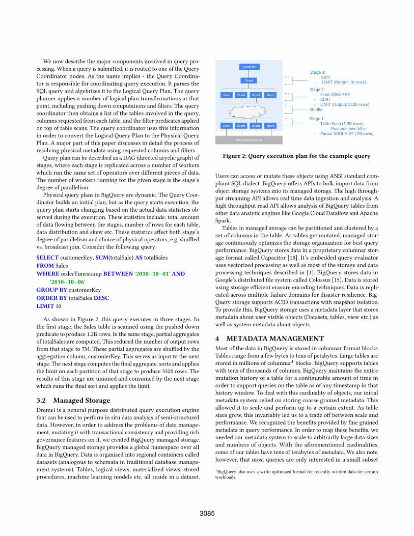
We now describe the major components involved in query pro-

cessing. When a query is submitted, it is routed to one of the Query

Coordinator nodes. As the name implies - the Query Coordina-

tor is responsible for coordinating query execution. It parses the

SQL query and algebrizes it to the Logical Query Plan. The query

planner applies a number of logical plan transformations at that

point, including pushing down computations and filters. The query

coordinator then obtains a list of the tables involved in the query,

columns requested from each table, and the filter predicates applied

on top of table scans. The query coordinator uses this information

in order to convert the Logical Query Plan to the Physical Query

Plan. A major part of this paper discusses in detail the process of

resolving physical metadata using requested columns and filters.

Query plan can be described as a DAG (directed acyclic graph) of

stages, where each stage is replicated across a number of workers

which run the same set of operators over different pieces of data.

The number of workers running for the given stage is the stage’s

degree of parallelism.

Physical query plans in BigQuery are dynamic. The Query Coor-

dinator builds an initial plan, but as the query starts execution, the

query plan starts changing based on the actual data statistics ob-

served during the execution. These statistics include: total amount

of data flowing between the stages, number of rows for each table,

data distribution and skew etc. These statistics affect both stage’s

degree of parallelism and choice of physical operators, e.g. shuffled

vs. broadcast join. Consider the following query:

SELECT customerKey, SUM(totalSale) AS totalSales

FROM Sales

WHERE orderTimestamp BETWEEN '2010−10−01' AND'2010−10−06'

GROUP BY customerKey

ORDER BY totalSales DESCLIMIT 10

As shown in Figure 2, this query executes in three stages. In

the first stage, the Sales table is scanned using the pushed down

predicate to produce 1.2B rows. In the same stage, partial aggregates

of totalSales are computed. This reduced the number of output rows

from that stage to 7M. These partial aggregates are shuffled by the

aggregation column, customerKey. This serves as input to the next

stage. The next stage computes the final aggregate, sorts and applies

the limit on each partition of that stage to produce 3320 rows. The

results of this stage are unioned and consumed by the next stage

which runs the final sort and applies the limit.

3.2 Managed StorageDremel is a general purpose distributed query execution engine

that can be used to perform in situ data analysis of semi-structured

data. However, in order to address the problems of data manage-

ment, mutating it with transactional consistency and providing rich

governance features on it, we created BigQuery managed storage.

BigQuery managed storage provides a global namespace over all

data in BigQuery. Data is organized into regional containers called

datasets (analogous to schemata in traditional database manage-

ment systems). Tables, logical views, materialized views, stored

procedures, machine learning models etc. all reside in a dataset.

Figure 2: Query execution plan for the example query

Users can access or mutate these objects using ANSI standard com-

pliant SQL dialect. BigQuery offers APIs to bulk import data from

object storage systems into its managed storage. The high through-

put streaming API allows real time data ingestion and analysis. A

high throughput read API allows analysis of BigQuery tables from

other data analytic engines like Google Cloud Dataflow and Apache

Spark.

Tables in managed storage can be partitioned and clustered by a

set of columns in the table. As tables get mutated, managed stor-

age continuously optimizes the storage organization for best query

performance. BigQuery stores data in a proprietary columnar stor-

age format called Capacitor [18]. It’s embedded query evaluator

uses vectorized processing as well as most of the storage and data

processing techniques described in [1]. BigQuery stores data in

Google’s distributed file system called Colossus [15]. Data is stored

using storage efficient erasure encoding techniques. Data is repli-

cated across multiple failure domains for disaster resilience. Big-

Query storage supports ACID transactions with snapshot isolation.

To provide this, BigQuery storage uses a metadata layer that stores

metadata about user visible objects (Datasets, tables, view etc.) as

well as system metadata about objects.

4 METADATA MANAGEMENTMost of the data in BigQuery is stored in columnar format blocks.

Tables range from a few bytes to tens of petabytes. Large tables are

stored in millions of columnar1blocks. BigQuery supports tables

with tens of thousands of columns. BigQuery maintains the entire

mutation history of a table for a configurable amount of time in

order to support queries on the table as of any timestamp in that

history window. To deal with this cardinality of objects, our initial

metadata system relied on storing coarse grained metadata. This

allowed it to scale and perform up to a certain extent. As table

sizes grew, this invariably led us to a trade off between scale and

performance. We recognized the benefits provided by fine grained

metadata in query performance. In order to reap these benefits, we

needed our metadata system to scale to arbitrarily large data sizes

and numbers of objects. With the aforementioned cardinalities,

some of our tables have tens of terabytes of metadata. We also note,

however, that most queries are only interested in a small subset

1BigQuery also uses a write optimized format for recently written data for certain

workloads.

3085

of columns. As a result of the columnar orientation of data, the

amount of I/O performed is a function of the size of data in the

columns referenced as opposed to the entire table size. We use this

same insight to drive our metadata design. Even though tables can

have tens of TB of metadata, the number of referenced columns

in any single query is general small. Thus, we use a columnar

representation for our metadata and we use our same proprietary

format, called Capacitor [18], to store it in. Using a columnar format

allows us to limit ourmetadata access also to the columns referenced

by the query.

Furthermore, analysis of our query patterns in BigQuery shows

that less than 10% of the queries either don’t have a filter or have a

filter that always evaluates to true. Based on our data, more than

60% of the queries select less than 1% of the data, and 25% percent

of the queries select less than 0.01% of the data. This suggests that

we can use these filters to eliminate the need for reading blocks

in addition to filtering out specific rows from within blocks. The

ability to eliminate partitions efficiently not only saves I/O cost but

also saves the cost of scheduling a partition on a worker.

4.1 Metadata structureWe classify storage metadata into two broad categories: Logical

metadata and Physical metadata. Logical metadata is information

about the table that is generally directly visible to the user. Some

examples of suchmetadata are: Table schema, Partitioning and Clus-

tering specifications, column and row level ACLs. This information

is generally small in size and lends itself to quick access. Physical

metadata is information about the table’s storage that BigQuery

maintains internally in order to map a table name to its actual data.

Examples of such information are: Locations of the blocks in the

file system, row counts, lineage of data in the blocks, MVCC in-

formation, statistics and properties of column values within each

block. If C is the number of columns in a table and N is the number

of blocks, the cardinality of column metadata is O(C × N). With C =

10K and N being of the order of millions, it is possible to have tens

of TB of metadata. It is clear that physical metadata, while being

extremely valuable for query execution, is not easily accessible. In

the rest of this paper, we focus on physical metadata, which we

simply refer to as “metadata”.

To solve this, we organize the physical metadata of each table

as a set of system tables that are derived from the original table.

To illustrate our idea, we describe the metadata layout using one

such system table (hereafter referred to as CMETA) that stores col-

umn level information about the min/max values (called range con-

straints), hash bucket and modulus values (called hash constraints)

and a dictionary of column values. Other variants of system tables

include those that store posting lists of column values. Query op-

timizer chooses one or more such system tables for planning and

executing the query.

Most of the data in a table is stored in columnar blocks on

Colossus. DML and other write operations such as bulk import

and streaming lead to the creation and deletion of rows in these

blocks. A block is considered active at a snapshot timestamp if it

contains at least one row that is visible at that timestamp. Blocks

with no visible rows remain in the system for a configurable amount

of time in order to support a feature known as “time travel” that al-

lows reading the table as of any given timestamp within the history

window. A query that reads this table needs to find the locations of

the blocks that are currently active in the table. Inside the blocks, it

is possible to have rows that are not visible at the timestamp. They

are filtered out when reading the block.

4.2 Columnar MetadataOur system table, hereafter referred to as CMETA, is organized

such that each row corresponds to a block in the table. We illustrate

the schema of the system table using our example Sales table from

Subsection 3.1.When building CMETA for a given table, we traverse

its [potentially] nested type structure to collect the “leaf” fields of

the nested types (i.e. ARRAY and STRUCT). The process of building

schema for CMETA can be described by the following recursive

algorithm which is applied to every column in the table:

• Type(ARRAY<T>) = Type(T)

• Type(STRUCT<𝑓1 𝑇1, ..., 𝑓𝑛 𝑇𝑛>)) = STRUCT<𝑓1 Type(𝑇1), ...,

𝑓𝑛 Type(𝑇𝑛)>

• For primitive types T, Type(T) = CMETATYPE<T> defined

as:

CREATE TYPE CMETATYPE<T> ASSTRUCT<total_rows INTEGER,total_nulls INTEGER,total_bytes INTEGER,min_value T,

max_value T,

hash STRUCT<bucket INTEGER,modulus INTEGER

>,

dictionary ARRAY<T>,

bloom_filter BYTES,s2_covering BYTES,...

>

Thus, CMETA’s schema for the Sales table is:

CREATE TABLE CMETA_Sales (

_block_locator BYTES,creation_timestamp TIMESTAMP,deletion_timestamp TIMESTAMP,block_total_bytes INTEGER,orderTimestamp CMETATYPE<TIMESTAMP>,salesOrderKey CMETATYPE<STRING>,customerKey CMETATYPE<STRING>,salesOrderLines STRUCT<

salesOrderLineKey CMETATYPE<INTEGER>,dueDate CMETATYPE<DATE>,shipDate CMETATYPE<DATE>,quantity CMETATYPE<INTEGER>,unitPrice CMETATYPE<NUMERIC>>,

3086

totalSale CMETATYPE<NUMERIC>,currencyKey CMETATYPE<INTEGER>>

)

CLUSTER BYorderTimestamp.max_value,

customerKey.max_value;

4.3 Incremental GenerationMutations (such as DML) that write to the original table, create

new blocks of data and/or mutate existing blocks of data. Thus, in

order for CMETA to be the source of truth for a table’s metadata, it

needs to be updated whenever the table is mutated. For simplicity of

exposition, we consider the block as the unit of mutation. In other

words, when data is modified, it is rewritten at block granularity.

Modification of any rows inside a block will cause a new block to

be created with the unmodified and modified rows while simul-

taneously marking the old block as deleted. In reality, BigQuery

contains blocks where only a subset of rows may be active at any

given timestamp. It is easy to see that our design below works for

partial blocks as well.

A metadata change log is used to journal the history of mutations

and additions of blocks. When a new block is created, we gather

the properties of the block, assign a creation timestamp (this is the

commit timestamp of the operation that is responsible for creation

of this block) and write an entry to the metadata change log. When

a block needs to be deleted, we write a log entry with the deletion

timestamp to the log. This change log is written to a highly available,

durable replicated storage system. Operations on table may create

and/or mutate millions of blocks, and the metadata change log

guarantees ACID properties for these mutations.

A background process constantly performs LSM[17] stylemerges

on the change log to produce baselines and deltas of changes. These

baselines and deltas are produced as columnar capacitor blocks

with the aforementioned schema. Note that baselines and deltas are

merged incrementally based on load and write rate to the change

log. At any given read timestamp, the table’s metadata can be con-

structed by reading the baseline available at that timestamp and

any deltas from the baseline up to the read timestamp.

Our incremental generation also works with high throughput

streaming ingestion as well. Data is received by ingestion servers

and persisted to a replicated write ahead log in Colossus. The most

recently streamed data is optimized by compacting into capacitor

blocks continuously. Fine grained metadata for rows that have

not yet been compacted into capacitor blocks is maintained in the

memory of ingestion servers.

5 QUERY PROCESSINGTo illustrate the use of CMETA for serving metadata, we use the

following query on the table from Subsection 4.2 as a running

example:

SELECT SUM(totalSale)

FROM Sales

WHERE orderTimestamp BETWEEN'2019−05−21 12:30:00' AND '2019−05−22 21:30:00'

A straightforward implementation of processing this querywould

be to open each block, perhaps use some metadata stored inside the

header of each block, apply the filter on that metadata and decide

whether or not this block needs processing. We describe our use

of distributed processing techniques to execute this query based

on CMETA that performs significantly better. We first describe our

query planning before going into query execution.

5.1 Query planningFor small tables which have a few tens of blocks, the cost of read-

ing the metadata is insignificant, but for tables with thousands

to millions of blocks, it turns out that loading the table metadata

naively before query planning increases the runtime of the query.

Depending on the size of the table, we observed added latencies

of tens of milliseconds (10GB+ tables) to tens of minutes (PB+ size

tables). To avoid this, we defer the reading of physical metadata

for the tables until the actual dispatch of partitions to the work-

ers. To facilitate this, the query planner first uses only the logical

metadata to generate a query plan with constants folded and filters

pushed down. Then, it rewrites the query plan as a semi-join of the

original query with CMETA over the _block_locator column. The

right side of the semi-join is a scan over the CMETA, optionally

containing a filter predicate derived (See Subsection 5.3) from fil-

ters in the original query. This query produces a list of locators of

blocks that need to be scanned in order to answer the query. The

constant start_timestamp is the snapshot timestamp at which the

query is being executed. In the case of a time travel read2, this is

the timestamp provided by the user.

SELECT _block_locator

FROM CMETA_Sales

WHEREorderTimestamp.min_value <= '2019−05−22 21:30:00'

ANDorderTimestamp.max_value >= '2019−05−21 12:30:00'

AND creation_timestamp <= start_timestamp

AND (deletion_timestamp IS NULLOR deletion_timestamp > start_timestamp)

Note that the list of block locators produced by this query may

contain some false positives. This does not affect the correctness

of the final query results, since the filter in the original query will

eliminate any extraneous rows. Assuming each row in the Sales

table to have the _block_locator virtual column, the original query

is rewritten3to:

SELECT SUM(totalSale)

FROM Sales

WHEREorderTimestamp

BETWEEN '2019−05−21 12:30:00' AND '2019−05−2221:30:00'

AND _block_locator IN (

SELECT _block_locator FROM CMETA_Sales

2https://cloud.google.com/bigquery/docs/time-travel

3We will present the algorithm for doing this rewrite in Subsection 5.3

3087

WHEREorderTimestamp.min_value <= '2019−05−22 21:30:00' ANDorderTimestamp.max_value >= '2019−05−21 12:30:00'

ANDcreation_timestamp <= start_timestamp AND(deletion_timestamp IS NULL ORdeletion_timestamp > start_timestamp )

The subquery over CMETA is evaluated first and it produces

the list of interesting blocks. These values are propagated to the

other side of the join which is the original query. Tables can have

millions of blocks, but only the blocks produced by the query on

the CMETA are processed by the original query. If the data in the

table is partitioned by ts, the number of blocks produced is several

orders of magnitude smaller than the total number of blocks in

the table. Additionally, the benefit of columnar metadata is evident

from the fact that even though T may have up to 10,000 columns,

the only columns read from it are:

• _block_locator

• orderTimestamp.min_value

• orderTimestamp.max_value

• creation_timestamp

• deletion_timestamp

5.2 Partition elimination and Falsifiableexpressions

Partition elimination is a popular technique to improve query per-

formance, by inspecting the filter condition and eliminating scan

of the partitions which cannot possibly satisfy the filter condition

[16]. Typically, partition elimination is limited to simple compari-

son predicates between single column and constants and checking

constants against min/max values of the block. In this section we

are going to present a generalized framework that applies to a rich

set of complex expressions, and can take advantage of a variety of

column statistics. Our approach is based on the notion of a falsi-fiable expression which is a boolean expression derived from the

query filters. It satisfies the following property:

For a given block, if the falsifiable expression evaluates to true, thatblock does not need to be scanned by the original query.

For any given filter condition, there exist many possible falsifiable

expressions. We determine the “quality" of falsifiable expressions

using the following two criteria:

• Complexity of expression: The formal definition of ex-

pression complexity is beyond the scope of this paper, but

informally x = ‘a’ is simpler than x LIKE ‘a%’

• Tightness: Falsifiable expression may (and in practice will)

have false negatives. i.e., there will be values for which it

will evaluate to 𝐹𝐴𝐿𝑆𝐸 - causing the block to be scanned.

However, subsequent application of the filter condition will

return 𝐹𝐴𝐿𝑆𝐸 for all values in the block. Falsifiable expres-

sion which doesn’t have false negatives is tight, while a

falsifiable expression with false positives is loose.

Our algorithm prefers falsifiable expressions which are less com-

plex but tighter. As an example, consider filter condition 𝑥 = 𝑐 ,

and block containing values 𝑐1, 𝑐2, ..., 𝑐𝑁 . Then the falsifiable ex-

pression 𝑐 <> 𝑐1 AND 𝑐 <> 𝑐2 AND ... AND 𝑐 <> 𝑐𝑁 is tight,

but potentially very complex for high values of N. The falsifiable

expression c NOT IN bloom_filter(𝑐1, ... 𝑐𝑁 ) is simpler, but less tight.

The falsifiable expression c > max(𝑐1, ..., 𝑐𝑁 ) OR c < min(𝑐1, ..., 𝑐𝑁 )

is potentially even less complex, but is looser.

5.3 Algorithm for building falsifiableexpressions

We now present our algorithm for converting a filter predicate in

the WHERE clause into a falsifiable expression.

Given:• A condition in the WHERE clause P(𝑥1, 𝑥2, ..., 𝑥𝑛) which

depends on variables 𝑥1, ..., 𝑥𝑛• Variables 𝑥1, ..., 𝑥𝑛 have corresponding CMETA’s column

properties 𝐶𝑋1, 𝐶𝑋2, ..., 𝐶𝑋𝑛 for given block

• Recall from Subsection 4.2, that column properties are of

type CMETATYPE<T> and contain various statistics about

values in the block:

CXi = {min(𝑥𝑖 ), max(𝑥𝑖 ), total_rows(𝑥𝑖 ), total_nulls(𝑥𝑖 ), ...}4

Goal:• Build a falsifiable expression 𝐹 (𝐶𝑋1,𝐶𝑋2, ...,𝐶𝑋𝑛), such that

when 𝐹 (𝐶𝑋1,𝐶𝑋2, ...,𝐶𝑋𝑛) evaluates to true, it is guaranteed

that no row in the block satisfies the condition 𝑃 (𝑥1, 𝑥2, ...,

𝑥𝑛), and therefore the block can be eliminated from the query

processing.

We can formally define the problem as: find 𝐹 (𝐶𝑋1,𝐶𝑋2, ...,𝐶𝑋𝑛)

such that

𝐹 (𝐶𝑋1, ...,𝐶𝑋𝑛) ⇒ ¬∃𝑥1, ..., 𝑥𝑛 (𝑃 (𝑥1, ..., 𝑥𝑛)) (1)

When falsifiable expression 𝐹 () is tight, the relationship is stronger,the absence of false negatives means that

¬𝐹 (𝐶𝑋1, ...,𝐶𝑋𝑛) ⇒ ∃𝑥1, ..., 𝑥𝑛 (𝑃 (𝑥1, ..., 𝑥𝑛))

and since ¬𝑝 ⇒ ¬𝑞 ≡ 𝑞 ⇒ 𝑝 , we can rewrite it as

¬∃𝑥1, ..., 𝑥𝑛 (𝑃 (𝑥1, ..., 𝑥𝑛)) ⇒ 𝐹 (𝐶𝑋1, ...,𝐶𝑋𝑛)

which together with Equation 1 gives us the following formal

definition of tight falsifiable expression:

𝐹 (𝐶𝑋1, ...,𝐶𝑋𝑛) ⇔ ¬∃𝑥1, ..., 𝑥𝑛 (𝑃 (𝑥1, ..., 𝑥𝑛)) (2)

Intuitively, this problem is related to the boolean satisfiability

problem, SAT5, even though the domain of variables extends beyond

boolean, and functions extend beyond boolean functions. Since SAT

is known to be NP-Complete, the problem of building a falsifiable

expression is NP-Complete as well. The algorithm we describe here

is only practical in a limited number of cases. However, it was

tuned to work well with conditions used in WHERE clauses that we

observed in actual representative workloads. We now present the

algorithm for building falsifiable expression 𝐹 (𝐶𝑋 ) for given expres-sion 𝑃 (𝑋 ) and CMETA properties 𝐶𝑋 . The algorithm is presented

as a collection of rules, which are applied recursively.

4for convenience, we will use min(𝑥𝑖 ) notation instead of CXi.min_value etc. through-

out the rest of the paper

5https://en.wikipedia.org/wiki/Boolean_satisfiability_problem

3088

5.3.1 Trival. Any arbitrary expression 𝑃 (𝑋 ), always has a falsifi-able expression 𝐹𝐴𝐿𝑆𝐸. The proof is trivial, since 𝐹𝐴𝐿𝑆𝐸 ⇒ 𝑃 (𝑋 )is a tautology. Of course, this falsifiable expression is not tight, and

seems to be not useful for partition elimination - it says that parti-

tion can never be eliminated - but it is important in that it serves

as a stop condition in the algorithm, when no other rules apply.

5.3.2 Conjunctions. Conjunction expressions are very common

in the WHERE clause of real-world SQL queries. They are auto-

matically generated by various visualization and BI tools when the

user chooses to filter on multiple attributes or dimensions; they

are produced by query planner rewrites, as planner pushes pred-

icates down to table scan and combines them with conjunction

operator; they can be generated as implementation of row level

security etc. We consider binary conjunction below, but it can be

easily generalized to n-ary conjunctions.

𝑃𝑋 (𝑋 ) AND 𝑃𝑌 (𝑌 )We have two expressions 𝑃𝑋 and 𝑃𝑌 over sets of variables X =

𝑥1, ... 𝑥𝑛 and Y = 𝑦1,..., 𝑦𝑘 respectively. We allow arbitrary overlaps

between X and Y, i.e. some of 𝑥𝑖 can be the same variables as 𝑦 𝑗 .

For example: they can be exactly the same variable: 𝑥 > 𝑐1 AND

𝑥 < 𝑐2. Or they can be completely disjoint: 𝑥 > 𝑐1 AND 𝑦 > 𝑐2.

If 𝑃𝑋 (𝑋 ) has falsifiable expression 𝐹𝑋 (𝐶𝑋 ), and 𝑃𝑌 (𝑌 ) has fal-sifiable expression 𝐹𝑌 (𝑌 ), then 𝑃𝑋 (𝑋 ) AND 𝑃𝑌 (𝑌 ) will have thefalsifiable expression 𝐹𝑋 (𝐶𝑋 ) OR 𝐹𝑌 (𝐶𝑌 ).

Proof. Given that

𝐹𝑋 (𝐶𝑋 ) ⇒ ¬∃𝑋 (𝑃𝑋 (𝑋 )) and 𝐹𝑌 (𝐶𝑌 ) ⇒ ¬∃𝑌 (𝑃𝑌 (𝑌 )), we needto prove that

𝐹𝑋 (𝐶𝑋 ) ∨ 𝐹𝑌 (𝐶𝑌 ) ⇒ ¬∃𝑋,𝑌 (𝑃𝑋 (𝑋 ) ∧ 𝑃𝑌 (𝑌 )).First, we note that since 𝑝 ⇒ 𝑞 ≡ ¬𝑞 ⇒ ¬𝑝 , we can derive that:

∃𝑋 (𝑃𝑋 (𝑋 )) ⇒ ¬𝐹𝑋 (𝐶𝑋 ) and ∃𝑌 (𝑃𝑌 (𝑌 )) ⇒ ¬𝐹𝑌 (𝐶𝑌 ).We start the proof with following statement:

∃𝑋,𝑌 (𝑃𝑋 (𝑋 ) ∧ 𝑃𝑌 (𝑌 )) ⇒∃𝑋 (𝑃𝑋 (𝑋 )) ∧ ∃𝑌 (𝑃𝑌 (𝑌 )) ⇒¬𝐹𝑋 (𝐶𝑋 ) ∧ ¬𝐹𝑌 (𝐶𝑌 ) ≡(𝐹𝑋 (𝐶𝑋 ) ∨ 𝐹𝑌 (𝐶𝑌 ))

We showed that:∃𝑋,𝑌 (𝑃𝑋 (𝑋 )∧𝑃𝑌 (𝑌 )) ⇒ ¬(𝐹𝑋 (𝐶𝑋 )∨𝐹𝑌 (𝐶𝑌 )and again applying 𝑝 ⇒ 𝑞 ≡ ¬𝑞 ⇒ ¬𝑝 we get:

𝐹𝑋 (𝐶𝑋 ) ∨ 𝐹𝑌 (𝐶𝑌 ) ⇒ ¬∃𝑋,𝑌 (𝑃𝑋 (𝑋 ) ∧ 𝑃𝑌 (𝑌 ))□

The resulting falsifiable expression we obtained is not tight even

if both 𝐹𝑋 and 𝐹𝑌 are tight. This is due to single directional impli-

cation at the first line of the proof.

5.3.3 Disjunctions. Expression 𝑃𝑋 (𝑋 ) OR 𝑃𝑌 (𝑌 ) has falsifiableexpressions 𝐹𝑋 (𝐶𝑋 ) AND 𝐹𝑌 (𝐶𝑌 ). The proof is very similar to the

conjunction case.

Proof.

∃𝑋,𝑌 (𝑃𝑋 (𝑋 ) ∨ 𝑃𝑌 (𝑌 )) ⇔∃𝑋 (𝑃𝑋 (𝑋 )) ∨ ∃𝑌 (𝑃𝑌 (𝑌 )) ⇒¬𝐹𝑋 (𝐶𝑋 ) ∨ 𝐹𝑌 (𝐶𝑌 ) ≡¬(𝐹𝑋 (𝐶𝑋 ) ∧ 𝐹𝑌 (𝐶𝑌 )) □

However, unlike conjunctions, the resulting falsifiable expression

is tight if 𝐹𝑋 and 𝐹𝑌 are both tight.

5.3.4 Comparisons between variable and constant. Table 1 shows afew examples of comparisons and their corresponding falsifiable

expressions (x is the variable, c is a constant). We provide a proof for

the first row in the table. We also prove that it is a tight falsifiable

expression.

Table 1: Variable and constant comparison

P() F()

x > c max(x) <= c

x < c min(x) >= c

x = c min(x) > c OR max(x) < c

x IS NOT NULL total_rows(x) = total_nulls(x)

x IS NULL total_nulls(x) = 0

etc.

Proof. We are given:

𝑃 (𝑥) = 𝑥 > 𝑐

𝐹 (𝐶𝑋 ) =𝑚𝑎𝑥 (𝑥) ≤ 𝑐

Wealso know from the definition ofmax(x) that∀𝑥 (𝑥 ≤ 𝑚𝑎𝑥 (𝑥)) ⇔𝑡𝑟𝑢𝑒

Therefore:

𝐹 (𝐶𝑋 ) ⇔ 𝐹 (𝐶𝑋 ) ∧ 𝑡𝑟𝑢𝑒∀𝑥 (𝑥 ≤ 𝑚𝑎𝑥 (𝑥)) ⇔𝑚𝑎𝑥 (𝑥) <= 𝑐 ∧ ∀𝑥 (𝑥 ≤ 𝑚𝑎𝑥 (𝑥)) ⇔∀𝑥 (𝑥 ≤ 𝑚𝑎𝑥 (𝑥) ∧𝑚𝑎𝑥 (𝑥) ≤ 𝑐) ⇔∀𝑥 (𝑥 ≤ 𝑐) ⇔ ∀𝑥¬(𝑥 > 𝑐) ⇔¬∃𝑥 (𝑥 > 𝑐) ⇔ ¬∃𝑥 (𝑃 (𝑥))We showed that 𝐹 (𝐶𝑋 ) ⇔ ¬∃𝑥 (𝑃 (𝑥)). This is the definition of

F(CX) being the tight falsifiable expression for p(x) from Equation 2.

□

Table 2 shows a few examples of falsifiable expressions produced

for multi-variable expressions.

Table 2: Multiple variables and constant comparisons

P() F()

𝑥1 > 𝑥2 max(𝑥1) <= min(𝑥2)

𝑥1 < 𝑥2 + 𝑐 min(𝑥1) >= max(𝑥2) + c

etc.

5.3.5 More complex comparisons. More complex comparisons can

be decomposed to simpler ones, e.g.

x BETWEEN 𝑐1 AND 𝑐2 ≡ x >= 𝑐1 AND x <= 𝑐2x IN (𝑐1, ..., 𝑐𝑁 ) x ≡ 𝑐1 OR ... OR x = 𝑐𝑁

and if we apply formulas from previous sections, we get the falsifi-

able expressions in Table 3.

With the IN expression, when 𝑁 is a large number, the resulting

falsifiable expression also becomes large and therefore more com-

plex. Alternatively, we can build a simpler but less tighter falsifiable

expression

3089

Table 3: Falsifiable expressions for complex SQL compar-isons

P() F()

x BETWEEN 𝑐1 AND 𝑐2 min(x) > 𝑐2 OR max(x) < 𝑐1

x IN (𝑐1, ..., 𝑐𝑁 ) (min(x) > 𝑐1 OR max(x) < 𝑐1) AND ...

AND (min(x) > 𝑐𝑁 OR max(x) < 𝑐𝑁 )

etc.

min(x) > max(𝑐1, ..., 𝑐𝑁 ) OR max(x) < min(𝑐1, ..., 𝑐𝑁 )

If CMETA has a bloom filter, it is possible to use it instead of min

and max, i.e.,

𝑐1 NOT IN bloom_filter(x) AND 𝑐2 NOT IN bloom_filter(x) AND ...

AND 𝑐𝑁 NOT IN bloom_filter(x)

5.3.6 Monotonic functions composition. If 𝑃 (𝑥) has falsifiable ex-pression 𝐹 (𝑚𝑖𝑛(𝑥),𝑚𝑎𝑥 (𝑥)) and𝐺 (𝑦) is monotonically non-decreasing

function, then: 𝑃 (𝐺 (𝑥)) will have a falsifiable expression𝐹 (𝐺 (𝑚𝑖𝑛(𝑥)),𝐺 (𝑚𝑎𝑥 (𝑥)).

Proof. First, we observe that for monotonic non-decreasing

function G(), the following is true:

𝐺 (𝑚𝑖𝑛(𝑥)) =𝑚𝑖𝑛(𝐺 (𝑥));𝐺 (𝑚𝑎𝑥 (𝑥)) =𝑚𝑎𝑥 (𝐺 (𝑥))To show it, we start with the definition of𝑚𝑖𝑛(𝑥) and the defini-

tion of the monotonic function:

∀𝑥 (𝑚𝑖𝑛(𝑥) <= 𝑥);∀𝑥1𝑥2 (𝑥1 <= 𝑥2 ⇒ 𝐺 (𝑥1) <= 𝐺 (𝑥2))Applying them together we will get:

∀𝑥 (𝑚𝑖𝑛(𝑥) <= 𝑥) ⇒ ∀𝑥 (𝐺 (𝑚𝑖𝑛(𝑥)) <= 𝐺 (𝑥))And the definition of min(G(x)): ∀𝑥 (𝑚𝑖𝑛(𝐺 (𝑥)) <= 𝐺 (𝑥)).

Therefore 𝐺 (𝑚𝑖𝑛(𝑥)) =𝑚𝑖𝑛(𝐺 (𝑥)) □

To illustrate this with an example, consider the following filter

condition:

DATE_TRUNC(d,MONTH) BETWEENDATE '2020−05−10' AND DATE '2020−10−20'

Here, DATE_TRUNC is monotonically increasing function 𝐺 (),and x BETWEEN DATE ’2020-05-10’ AND DATE ’2020-10-20’ is

the comparison function 𝑃 (). Therefore, the falsifiable expressionwould be:

DATE_TRUNC(min(d),MONTH) > DATE_TRUNC(DATE'2020−10−20')

ORDATE_TRUNC(max(d), MONTH) < DATE_TRUNC(DATE

'2020−05−10')

which is

DATE_TRUNC(min(d),MONTH) > DATE '2020−10−01' ORDATE_TRUNC(max(d),MONTH) < DATE '2020−05−01'

5.3.7 Conditional monotonicity. Certain functions are provably

monotonic only for a subset of values in the domain of the func-

tion. We introduce additional conditions in the generated falsifiable

functions. If 𝑃 (𝑥) has falsifiable expression 𝐹 (𝑚𝑖𝑛(𝑥),𝑚𝑎𝑥 (𝑥)) and

𝐺 (𝑦) is monotonically non-decreasing function in the domain of val-

ues of 𝐺 () only when the condition 𝐻 (𝐶𝑋 ) is true, then: 𝑃 (𝐺 (𝑥))will have the falsifiable function 𝐹 (𝐺 (𝑚𝑖𝑛(𝑥)),𝐺 (𝑚𝑎𝑥 (𝑥)) AND𝐻 (𝐶𝑋 ).

The astute reader will note that many datetime manipulation

functions are not monotonic. Consider the following function for

instance over variable x of type DATE:

FORMAT_DATE('%Y%m', x) = '201706'

The generated falsifiability expression based only on subsubsec-

tion 5.3.6 is:

FORMAT_DATE('%Y%m',max(x)) < '201706' ORFORMAT_DATE('%Y%m',min(x)) > '201706'

However, this function is not monotonic over the possible range of

values of x [‘0001-01-01’, ‘9999-12-31’]. If a block has min(x) = DATE

‘917-05-12’ (a date in the calendar year 917 AD), and max(x) = DATE

‘2019-05-25’, then, the above falsifiable expression will eliminate

the block from query processing, even though it can contain a

row that satisfies the filter. We apply a condition for pruning that

requires timestamps in a block to be in or after the year 1000 AD.

The generated falsifiable expression is:

(FORMAT_DATE('%Y%m',max(x)) < '201706'OR FORMAT_DATE('%Y%m',min(x)) > '201706')AND EXTRACT(YEAR FROMmin(x)) >= 1000

5.3.8 Array functions. When x is of type array, WHERE clause

condition can contain subqueries and correlated semi-joins, i.e.

EXISTS(SELECT ... FROM UNNEST(x) AS xs

WHERE ps(xs))

or

(SELECT LOGICAL_OR(ps(xs)) FROM UNNEST(x) AS xs)

where ps(x) is a function applied to the elements of the array x.

Falsifiable expressions will then be computed for ps(x). For example:

EXISTS(SELECT ∗ FROM UNNEST(x) AS xsWHERE xs > 5)

after applying rules from previous sections will result in the falsifi-

able expression: max(x) <= 5

Another example is:

c IN (SELECT xs FROM UNNEST(x) AS xs)

It is equivalent to

EXISTS(SELECT ∗ FROM UNNEST(x) AS xsWHERE xs = c)

Here ps(x) is x = c, and falsifiable expression will be: c < min(x)

OR c > max(x)

5.3.9 Rewrites. Sometimes it is possible to rewrite expressions to

fit one of the above forms. An exhaustive list of such rewrites is

outside of the scope of this paper, but we show a few examples. In

the general case, if we know that p() has falsifiable expression f(),

3090

we cannot derive a falsifiable expression for NOT p(). Therefore, we

apply algebraic transformations to eliminate negations whenever

possible. Table 4 shows list of such transformations.

Table 4: Expression rewrites to eliminate negations

Expression with NOT Rewrite

NOT(p OR q) (NOT p) AND (NOT q)

NOT(p AND q) (NOT p) OR (NOT q)

NOT (x < c) (x >= c)

NOT (x = c) (x <> c)

NOT (x IS NULL) (x IS NOT NULL)

etc.

Table 5 shows examples of arithmetic transformations for nu-

meric and datetime types.

Table 5: Arithmetic expressions

Expression Rewrite

x + 𝑐1 > 𝑐2 x > (𝑐2 - 𝑐1)

DATE_SUB(x, 𝑐1) < 𝑐2 x < DATE_ADD(𝑐2, 𝑐1)

etc.

Table 6 shows how string prefix matching functions can be

rewritten as comparisons.

Table 6: String functions

Expression Rewrite

x LIKE ‘c%’

x >= ‘c’ AND x < ‘d’

REGEXP(x, ‘c.*’)

STARTS_WITH(x, ‘c’)

5.3.10 Geospatial functions. GEOGRAPHY is an interesting type,

because it doesn’t have linear ordering, and so there is no notion

of min and max values for columns of this type. Instead, CMETA

column properties for the values of type GEOGRAPHY include the

S2 covering cells [20] of all values in the block. Each S2 cell repre-

sents a part of the Earth’s surface at different levels of granularity.

S2 cell at level 0 is about 85 million 𝑘𝑚2, while S2 cell at level 30 is

about 1𝑐𝑚2. Figure 3 shows an example of S2 covering using eight

S2 cells at levels 15 to 18. Each S2 cell is uniquely encoded as 64-bit

unsigned integer. The more cells the covering has - the more tightly

it can cover the objects in the block, but at the expense of using

more space.

The covering can be used together with special internal functions

to derive falsifiable expression. For example, for the filter condition

ST_INTERSECTS(x, constant_geo)

the falsifiable expression would be:

NOT _ST_INTERSECTS(

s2_covering(constant_geo) , s2_covering(x) )

Figure 3: S2 cells covering of The Metropolitan Museum ofArts in New York

where _ST_INTERSECTS is an internal function, which returns

𝑇𝑅𝑈𝐸 if two S2 coverings intersect (and therefore there is a possi-

bility that objects that they cover may intersect as well).

5.3.11 Same value in the block. An interesting special case is presentwhen all values of a variable in the block are the same (i.e. min(x)

= max(x)) or NULLs. In this case, we can calculate P(min(x)) and

P(NULL) and check if the result is 𝐹𝐴𝐿𝑆𝐸 or NULL - both of which

eliminate rows: 𝐹 (𝐶𝑋 ) = (NOT 𝑃 (𝐶𝑋 )) OR (𝑃 (𝐶𝑋 ) IS NULL) AND𝑚𝑖𝑛(𝑥) =𝑚𝑎𝑥 (𝑥).

This works for arbitrary complex functions 𝑃 (), as long as it

is known to be deterministic (i.e., it won’t work for RAND() or

non-deterministic UDF). However, adding this condition to every

variable in falsifiable expression makes it costlier. In the common

case, since most columns don’t have the same value in an entire

block, this is wasteful. An exception to this is when we have addi-

tional metadata information – for example partitioning key column

of type DATE and data partitioned on date granularity. Since blocks

in BigQuery don’t cross partition boundaries, blocks are guaranteed

to have the same value for the partitioning key.

5.4 Query rewrite using CMETA and falsifiableexpression

We now show how the falsifiable expression is used in a query

rewrite. Given the following user written query:

SELECT 𝑦1, 𝑦2, . . . 𝑦𝑘 FROM T WHERE 𝑃 (𝑥1, 𝑥2, ..., 𝑥𝑛)

We generate the falsifiable expression 𝐹 (𝐶𝑋1, 𝐶𝑋2, ..., 𝐶𝑋𝑛) from

the WHERE clause P. Since blocks can be eliminated when 𝐹 ()evaluates to 𝑇𝑅𝑈𝐸, we can get a list of interesting blocks with

following CMETA scan:

SELECT _block_locator FROM CMETA

WHERE NOT F(𝐶𝑋1, 𝐶𝑋2, ..., 𝐶𝑋𝑛)

Using it in a semi-join with the original user query, we get the

following query:

SELECT _block_locator, ∗ FROM(SELECT 𝑦1, 𝑦2,..., 𝑦𝑘 FROM TWHERE P(𝑥1, 𝑥2, ..., 𝑥𝑛))

WHERE _block_locator IN(SELECT _block_locator FROM CMETA_T

WHERE NOT F(𝐶𝑋1, 𝐶𝑋2, ..., 𝐶𝑋𝑛))

3091

5.5 Processing JoinsStar and snowflake schemas are commonly found in data ware-

houses. Typically, in such schemas, many queries filter data from

large fact tables based on filters on dimension tables. The dimension

tables are small, and typically don’t need parallel scans. Queries

may explicitly contain filters only on the dimension table. The

straightforward approach of using a system table to generate the

list of blocks to scan for the fact table is not very effective because

the query doesn’t have a statically specified filter over it. Sideways

information passing [11] is a common query optimization strategy

used for improving performance of joins. As the query executes,

we use the information from the dimension table scan to generate

a filter expression on the fact table. We delay the processing of the

system metadata table for the fact table until such filter expression

has been computed. Once the implied filter expression has been

computed, we push that filter into the fact table scan. As a result,

we are able to scan the fact table’s CMETA system table exactly

as if the filter were specified statically. To illustrate, consider the

following example query, based on TPC-DS subqueries #9 and #10,

against the Sales fact table from Subsection 4.2 and the dimension

table DateDim with fields: dt, year and monthOfYear:

SELECT SUM(Sales.totalSale)

FROM Sales, DateDim

WHERE DATE(Sales.orderTimestamp) = DateDim.dt

AND DateDim.year = 2017

AND DateDim.monthOfYear between 1 AND 2

The DateDim table is very small – 10 years worth of dates take

only 3660 rows. During execution, we first scan the DateDim table

with the provided filter on fields “year” and “monthOfYear”. The

result of this query is used to derive additional filters on the fact

table. For example, this can yield a range of values for “dt” that can

be condensed into a range of dates [dt_min, dt_max]. This in turn

leads to the following derived filter expression on the Sales table:

WHERE DATE(orderTimestamp) BETWEEN dt_min ANDdt_max

At this point, our algorithms for Subsection 5.3 can be applied to

this derived filter expression to generate a falsifiable expression.

The final query generated over CMETA for Sales table is:

SELECT _block_locator

FROM CMETA_Sales

WHERE DATE(orderTimestamp.max_value) >= dt_min

AND DATE(orderTimestamp.min_value) <= dt_max

Large fact tables have millions of blocks and just finding the

relevant blocks to scan is a bottleneck. Filters of the kind mentioned

above are often selective. If the Sales table is partitioned or clustered

on the orderTimestamp column, this approach leads to orders of

magnitude improvement in query performance.

5.6 Query OptimizationThere are multiple optimizations BigQuery’s planner can apply

based on the shape of the data. The most fundamental one is choos-

ing the degree of parallelism for different stages of the query execu-

tion.More complex ones allow it to choose different query execution

plans. For example, consider choosing the join strategy, i.e. broad-

cast vs hash join. Broadcast join doesn’t need to shuffle data on the

large side of the join so can be considerably faster, but broadcast

only works for small datasets that fit in memory. Generally, it is

difficult to obtain accurate cardinality estimates during query plan-

ning; it is well-known that errors propagate exponentially through

joins [10]. BigQuery has chosen a path where the query execution

plan can dynamically change during runtime based on the signals

about the data shape. However, in order for the dynamic adaptive

scheme to work well in practice, the initial estimates should be close

to the actual numbers. Query planner uses per column statistics

from CMETA to make these estimates. A query’s estimated size

is calculated by adding the number of bytes that will be scanned

from each table based on the referenced fields and the blocks that

remain after partitions have been eliminated by pruning. CMETA

allows us to compute such information for the user written query

efficiently using the following query:

SELECTSUM(𝐶𝑌1.total_bytes) + ... + SUM(𝐶𝑌𝑘 .total_bytes) +

SUM(𝐶𝑋1.total_bytes) + ... + SUM(𝐶𝑋𝑛 .total_bytes)

FROM CMETA_T

WHERE NOT F(𝐶𝑋1, 𝐶𝑋2, ..., 𝐶𝑋𝑛)

In fact, BigQuery has a "dry-run" feature, which allows the user

to estimate the amount of data scanned without actually executing

the query. This is quite useful, because it allows users to set cost

controls on queries over such large tables. An example of such cost

control is: "Execute this query only if it processes less than X GB".

The above query over CMETA can be used to support it.

The optimizer transparently rewrites subtrees of the query plan

to use materialized views where possible. When multiple material-

ized views are viable for use in a query, the optimizer has to choose

the best one for performance and cost. It does so by estimating the

query size of the subtree for each of the materialized views by using

CMETA for the materialized views.

5.7 Interleaved processingWhile the queries over selective filters eliminate a lot of blocks,

we optimize CMETA to work on queries without selective filters.

Processing a large table may require reading a large number of rows

from CMETA. Since we process CMETA in a distributed manner,

scanning it is massively parallelized. Collecting all the metadata

on the query coordinator before dispatching individual partitions

of the query is prohibitive in terms of memory usage as well as

in added latency on the critical path of a query. Our design scales

to such queries by interleaving the execution of the scan over

CMETA with the execution of the actual query. As the scan over

CMETA produces rows which contain block locators, they are used

to dispatch partitions for the main table to the workers.

3092

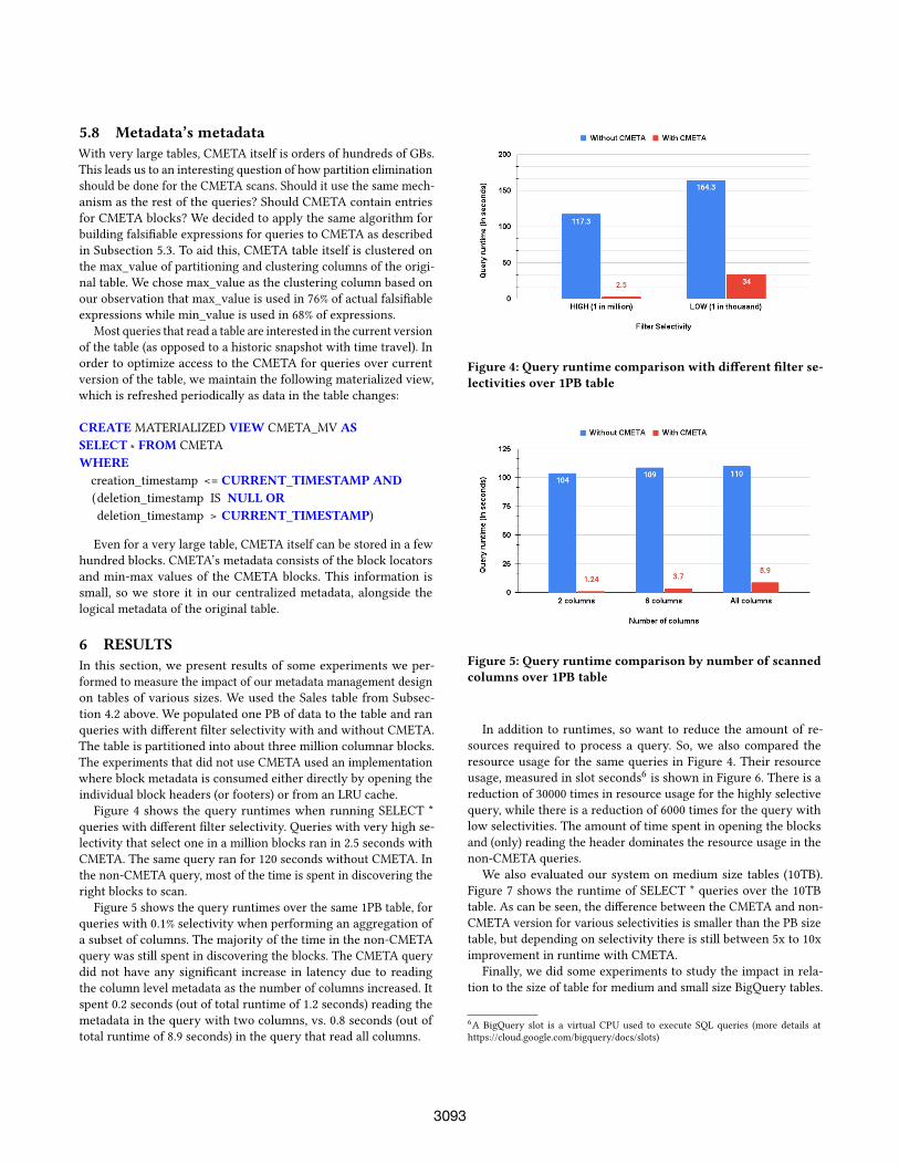
5.8 Metadata’s metadataWith very large tables, CMETA itself is orders of hundreds of GBs.

This leads us to an interesting question of how partition elimination

should be done for the CMETA scans. Should it use the same mech-

anism as the rest of the queries? Should CMETA contain entries

for CMETA blocks? We decided to apply the same algorithm for

building falsifiable expressions for queries to CMETA as described

in Subsection 5.3. To aid this, CMETA table itself is clustered on

the max_value of partitioning and clustering columns of the origi-

nal table. We chose max_value as the clustering column based on

our observation that max_value is used in 76% of actual falsifiable

expressions while min_value is used in 68% of expressions.

Most queries that read a table are interested in the current version

of the table (as opposed to a historic snapshot with time travel). In

order to optimize access to the CMETA for queries over current

version of the table, we maintain the following materialized view,

which is refreshed periodically as data in the table changes:

CREATEMATERIALIZED VIEW CMETA_MV ASSELECT ∗ FROM CMETA

WHEREcreation_timestamp <= CURRENT_TIMESTAMP AND(deletion_timestamp IS NULL ORdeletion_timestamp > CURRENT_TIMESTAMP)

Even for a very large table, CMETA itself can be stored in a few

hundred blocks. CMETA’s metadata consists of the block locators

and min-max values of the CMETA blocks. This information is

small, so we store it in our centralized metadata, alongside the

logical metadata of the original table.

6 RESULTSIn this section, we present results of some experiments we per-

formed to measure the impact of our metadata management design

on tables of various sizes. We used the Sales table from Subsec-

tion 4.2 above. We populated one PB of data to the table and ran

queries with different filter selectivity with and without CMETA.

The table is partitioned into about three million columnar blocks.

The experiments that did not use CMETA used an implementation

where block metadata is consumed either directly by opening the

individual block headers (or footers) or from an LRU cache.

Figure 4 shows the query runtimes when running SELECT *

queries with different filter selectivity. Queries with very high se-

lectivity that select one in a million blocks ran in 2.5 seconds with

CMETA. The same query ran for 120 seconds without CMETA. In

the non-CMETA query, most of the time is spent in discovering the

right blocks to scan.

Figure 5 shows the query runtimes over the same 1PB table, for

queries with 0.1% selectivity when performing an aggregation of

a subset of columns. The majority of the time in the non-CMETA

query was still spent in discovering the blocks. The CMETA query

did not have any significant increase in latency due to reading

the column level metadata as the number of columns increased. It

spent 0.2 seconds (out of total runtime of 1.2 seconds) reading the

metadata in the query with two columns, vs. 0.8 seconds (out of

total runtime of 8.9 seconds) in the query that read all columns.

Figure 4: Query runtime comparison with different filter se-lectivities over 1PB table

Figure 5: Query runtime comparison by number of scannedcolumns over 1PB table

In addition to runtimes, so want to reduce the amount of re-

sources required to process a query. So, we also compared the

resource usage for the same queries in Figure 4. Their resource

usage, measured in slot seconds6is shown in Figure 6. There is a

reduction of 30000 times in resource usage for the highly selective

query, while there is a reduction of 6000 times for the query with

low selectivities. The amount of time spent in opening the blocks

and (only) reading the header dominates the resource usage in the

non-CMETA queries.

We also evaluated our system on medium size tables (10TB).

Figure 7 shows the runtime of SELECT * queries over the 10TB

table. As can be seen, the difference between the CMETA and non-

CMETA version for various selectivities is smaller than the PB size

table, but depending on selectivity there is still between 5x to 10x

improvement in runtime with CMETA.

Finally, we did some experiments to study the impact in rela-

tion to the size of table for medium and small size BigQuery tables.

6A BigQuery slot is a virtual CPU used to execute SQL queries (more details at

https://cloud.google.com/bigquery/docs/slots)

3093

Figure 6: Resource usage comparison for different filter se-lectivities over 1PB table

Figure 7: Query runtime comparison with different filter se-lectivities over 10TB table

Figure 8 shows the query runtime for different table sizes. As ta-

ble sizes become smaller, the difference in query runtime reduces

between non-CMETA based and CMETA based query processing.

Figure 8: Query runtime comparison for different table sizes

7 CONCLUSIONS AND FUTUREWORKIn this paper, we described a variety of ways that we have used

the rich metadata information stored in CMETA during query pro-

cessing. Our techniques are based on the intuition that metadata

management at scale is not fundamentally different from data man-

agement. We recognize the power of distributed processing for

data management and devise our algorithms to integrate metadata

processing into query execution. Experimental results demonstrate

that CMETA improves query performance and resource utilization

by several orders of magnitude, and the improvements are more

pronounced at larger data sizes. We believe that our techniques

have broader applicability in many other scenarios. We present

some possible areas of future work for us below.

We are exploring the use of CMETA to drive range partitioned

joins. When a large clustered table is joined with another small

to medium sized table on its clustering columns, the smaller side

often cannot be broadcast to the other. In such cases, we can avoid

the expensive shuffling of the large table by using the clustering

column’s properties from CMETA.We can gather the block locators

and their corresponding min-max values for the clustering columns

by performing a distributed scan on the large table. The smaller side

can then be range partitioned using these min-max values. Once

shuffled, the join can be performed by appropriately pairing blocks

from the large table with the partitions written to shuffle.

We started with the premise that metadata is too large to fit in

memory, and thus it needs to use distributed processing techniques

similar to big data. There is no doubt that if we were able to store all

of this metadata in memory, we could get a significant performance

boost. This is obviously prohibitive in terms of cost as well as scal-

ability. We believe that we can get the best of both worlds, infinite

scalability and in-memory processing speeds, by caching the work-

ing set. CMETA’s columnar design lends itself well to column level

caching of metadata in memory. In our experiments, scanning the

metadata of the petabyte table took 500ms. By caching the metadata

stored in CMETA for hot columns and using vectorized processing,

performance of CMETA scans can be significantly accelerated.

ACKNOWLEDGMENTSWe would like to sincerely thank the reviewers of the drafts of this

paper: Sam McVeety, Magdalena Balazinska, Fatma Ozcan and Jeff

Shute. We would like to acknowledge code contributions made by

the following engineers: Adrian Baras, Aleksandras Surna, Eugene

Koblov, Hua Zhang, Nhan Nguyen, Stepan Yakovlev, Yunxiao Ma.

REFERENCES[1] Daniel Abadi, Samuel Madden, and Miguel Ferreira. 2006. Integrating Compres-

sion and Execution in Column-Oriented Database Systems. In Proceedings of the2006 ACM SIGMOD International Conference on Management of Data (Chicago,IL, USA) (SIGMOD ’06). Association for Computing Machinery, New York, NY,

USA, 671–682. https://doi.org/10.1145/1142473.1142548

[2] Sunil Agarwal. 2017. Columnstore Index Performance: Rowgroup Elimina-tion. https://techcommunity.microsoft.com/t5/sql-server/columnstore-index-

performance-rowgroup-elimination/ba-p/385034

[3] Michael Armbrust, Tathagata Das, Liwen Sun, Burak Yavuz, Shixiong Zhu, Mukul

Murthy, Joseph Torres, Herman van Hovell, Adrian Ionescu, Alicja undefine-

duszczak, Michał undefinedwitakowski, Michał Szafrański, Xiao Li, Takuya

Ueshin, Mostafa Mokhtar, Peter Boncz, Ali Ghodsi, Sameer Paranjpye, Pieter

Senster, Reynold Xin, and Matei Zaharia. 2020. Delta Lake: High-Performance

ACID Table Storage over Cloud Object Stores. 13, 12 (Aug. 2020), 3411–3424.

https://doi.org/10.14778/3415478.3415560

3094

[4] Jesús Camacho-Rodríguez, Ashutosh Chauhan, Alan Gates, Eugene Koifman,

Owen O’Malley, Vineet Garg, Zoltan Haindrich, Sergey Shelukhin, Prasanth Jay-

achandran, Siddharth Seth, Deepak Jaiswal, Slim Bouguerra, Nishant Bangarwa,

Sankar Hariappan, Anishek Agarwal, Jason Dere, Daniel Dai, Thejas Nair, Nita

Dembla, Gopal Vijayaraghavan, and Günther Hagleitner. 2019. Apache Hive:

From MapReduce to Enterprise-Grade Big Data Warehousing. In Proceedings ofthe 2019 International Conference on Management of Data (Amsterdam, Nether-

lands) (SIGMOD ’19). Association for Computing Machinery, New York, NY, USA,

1773–1786. https://doi.org/10.1145/3299869.3314045

[5] Fay Chang, JeffreyDean, SanjayGhemawat,Wilson C. Hsieh, DeborahA.Wallach,

Mike Burrows, Tushar Chandra, Andrew Fikes, and Robert E. Gruber. 2006.

Bigtable: A distributed storage system for structured data. In IN PROCEEDINGSOF THE 7TH CONFERENCE ON USENIX SYMPOSIUM ON OPERATING SYSTEMSDESIGN AND IMPLEMENTATION - VOLUME 7. 205–218.

[6] Zach Christopherson. 2016. Amazon Redshift Engineering’s Advanced Table DesignPlaybook: Compound and Interleaved Sort Keys. https://amzn.to/3qXXVpq

[7] Benoit Dageville, Thierry Cruanes, Marcin Zukowski, Vadim Antonov, Artin

Avanes, Jon Bock, Jonathan Claybaugh, Daniel Engovatov, Martin Hentschel,

Jiansheng Huang, AllisonW. Lee, Ashish Motivala, Abdul Q. Munir, Steven Pelley,

Peter Povinec, Greg Rahn, Spyridon Triantafyllis, and Philipp Unterbrunner. 2016.

The Snowflake Elastic Data Warehouse. In Proceedings of the 2016 InternationalConference on Management of Data (San Francisco, California, USA) (SIGMOD’16). Association for Computing Machinery, New York, NY, USA, 215–226. https:

//doi.org/10.1145/2882903.2903741

[8] Anurag Gupta, Deepak Agarwal, Derek Tan, Jakub Kulesza, Rahul Pathak, Ste-

fano Stefani, and Vidhya Srinivasan. 2015. Amazon Redshift and the Case for

Simpler Data Warehouses. In Proceedings of the 2015 ACM SIGMOD InternationalConference on Management of Data (Melbourne, Victoria, Australia) (SIGMOD’15). Association for Computing Machinery, New York, NY, USA, 1917–1923.

https://doi.org/10.1145/2723372.2742795

[9] HMS 2020. Hive Metastore (HMS). https://docs.cloudera.com/documentation/

enterprise/latest/topics/cdh_ig_hms.html

[10] Yannis E. Ioannidis and Stavros Christodoulakis. 1991. On the Propagation

of Errors in the Size of Join Results. In Proceedings of the 1991 ACM SIGMODInternational Conference on Management of Data (Denver, Colorado, USA) (SIG-MOD ’91). Association for Computing Machinery, New York, NY, USA, 268–277.

https://doi.org/10.1145/115790.115835

[11] Zachary G. Ives and Nicholas E. Taylor. 2008. Sideways Information Passing for

Push-Style Query Processing. In Proceedings of the 2008 IEEE 24th InternationalConference on Data Engineering (ICDE ’08). IEEE Computer Society, USA, 774–783.

https://doi.org/10.1109/ICDE.2008.4497486

[12] Andrew Lamb, Matt Fuller, Ramakrishna Varadarajan, Nga Tran, Ben Vandiver,

Lyric Doshi, and Chuck Bear. 2012. The Vertica Analytic Database: C-Store 7

Years Later. Proc. VLDB Endow. 5, 12 (Aug. 2012), 1790–1801. https://doi.org/10.

14778/2367502.2367518

[13] Sergey Melnik, Andrey Gubarev, Jing Jing Long, Geoffrey Romer, Shiva Shiv-

akumar, Matt Tolton, Theo Vassilakis, Hossein Ahmadi, Dan Delorey, Slava

Min, Mosha Pasumansky, and Jeff Shute. 2020. Dremel: A Decade of Interactive

SQL Analysis at Web Scale. Proc. VLDB Endow. 13, 12 (Aug. 2020), 3461–3472.https://doi.org/10.14778/3415478.3415568

[14] Sergey Melnik, Andrey Gubarev, Jing Jing Long, Geoffrey Romer, Shiva Shivaku-

mar, Matt Tolton, Theo Vassilakis, and Google Inc. 2010. Dremel: Interactive

Analysis of Web-Scale Datasets.

[15] Cade Metz. 2012. Google Remakes Online Empire with ’Colossus’.[16] Guido Moerkotte. 1998. Small Materialized Aggregates: A Light Weight Index

Structure for Data Warehousing. In Proceedings of the 24rd International Confer-ence on Very Large Data Bases (VLDB ’98). Morgan Kaufmann Publishers Inc., San

Francisco, CA, USA, 476–487.

[17] Patrick O’Neil, Edward Cheng, Dieter Gawlick, and Elizabeth O’Neil. 1996. The

Log-Structured Merge-Tree (LSM-Tree). Acta Inf. 33, 4 (June 1996), 351–385.

https://doi.org/10.1007/s002360050048

[18] Mosha Pasumansky. 2016. Inside Capacitor, BigQuery’s Next-

Generation Columnar Storage Format. Google Cloud Blog, Apr 2016.

https://cloud.google.com/blog/products/bigquery/inside-capacitor-bigquerys-

next-generation-columnar-storage-format

[19] Vijayshankar Raman, Gopi Attaluri, Ronald Barber, Naresh Chainani, David

Kalmuk, Vincent KulandaiSamy, Jens Leenstra, Sam Lightstone, Shaorong Liu,

Guy M. Lohman, Tim Malkemus, Rene Mueller, Ippokratis Pandis, Berni Schiefer,

David Sharpe, Richard Sidle, Adam Storm, and Liping Zhang. 2013. DB2 with

BLU Acceleration: So Much More than Just a Column Store. Proc. VLDB Endow.6, 11 (Aug. 2013), 1080–1091. https://doi.org/10.14778/2536222.2536233

[20] S2 Cells [n.d.]. S2 Cells. https://s2geometry.io/devguide/s2cell_hierarchy.html

3095