
BIG DATA FOR SAFETY MONITORING, ASSESSMENT, AND IMPROVEMENT · researchers’ understanding of the...
125
BIG DATA FOR SAFETY MONITORING, ASSESSMENT, AND IMPROVEMENT FINAL REPORT Southeastern Transportation Center MOHAMED ABDEL-ATY ESSAM RADWAN JAEYOUNG LEE LING WANG QI SHI SEPTEMBER 2016 US Department of Transportation grant DTRT13-G-UTC34
Transcript of BIG DATA FOR SAFETY MONITORING, ASSESSMENT, AND IMPROVEMENT · researchers’ understanding of the...
BIGDATAFORSAFETYMONITORING,
ASSESSMENT,ANDIMPROVEMENT
FINALREPORT
SoutheasternTransportationCenter
MOHAMEDABDEL-ATY
ESSAMRADWAN
JAEYOUNGLEE
LINGWANG
QISHI
SEPTEMBER2016
USDepartmentofTransportationgrantDTRT13-G-UTC34

DISCLAIMER
The contents of this report reflect the views of the authors,
who are responsible for the facts and the accuracy of the
information presented herein. This document is disseminated
under the sponsorship of the Department of Transportation,
University Transportation Centers Program, in the interest of
information exchange. The U.S. Government assumes no
liability for the contents or use thereof.
1. Report No. 2. Government Accession No.
3. Recipient’s Catalog No.
4. Title and Subtitle Big Data for Safety Monitoring, Assessment, and Improvement
5. Report Date September 2016
6. Source Organization Code Budget
7. Author(s) Abdel-Aty, Dr. Mohamed; Radwan, Dr. Ahmed; Lee, Dr. JaeYoung; Wang, Dr. Ling; Shi, Dr. Qi
8. Source Organization Report No. STC-2015-##-XX
9. Performing Organization Name and Address 10. Work Unit No. (TRAIS)
Southeastern Transportation Center UT Center for Transportation Research 309 Conference Center Building Knoxville TN 37996-4133
11. Contract or Grant No. DTRT13-G-UTC34
12. Sponsoring Agency Name and Address
US Department of Transportation Office of the Secretary of Transportation–Research 1200 New Jersey Avenue, SE Washington, DC 20590
13. Type of Report and Period Covered Final Report: May 2014 – October 2016
14. Sponsoring Agency Code USDOT/OST-R/STC
15. Supplementary Notes:
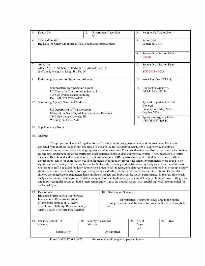
16. Abstract
This project implemented big data for traffic safety monitoring, assessment, and improvement. Data were collected from multiple sources and integrated to explore the traffic safety mechanisms of expressway mainlines, expressway ramps, expressway weaving segments, and intersections. Data visualization was first carried out for facilitating researchers’ understanding of the traffic and crash patterns on the studied expressway system. Then, based on big traffic data, a well-calibrated and validated microscopic simulation VISSIM network was built to find the real-time conflict contributing factors for expressway weaving segments. Additionally, travel time reliability parameters were found to be significant traffic safety contributing factors for both crash frequency and real-time safety analysis studies. In addition to microscopic traffic data and roadway geometric characteristics, macroscopic data were also attempted in microscopic safety studies: real-time crash analysis for expressway ramps and safety performance functions for intersections. The results showed that macroscopic parameters had significant impacts and improved the model performance. In the real-time crash analysis for ramps, the integration of data mining method and traditional statistic model largely eliminated over fitting issue and improved model accuracy. In the intersection safety study, the optimal macro-level spatial unit was recommended for each crash type.
17. Key Words
Big data; Traffic safety; Expressway; Intersections; Data visualization; Microscopic simulation VISSIM; Travel time reliability; Real-time safety analysis; Safety performance function
18. Distribution Statement
Unrestricted; Document is available to the public through the National Technical Information Service; Springfield, VT.
19. Security Classif. (of this report)
Unclassified
20. Security Classif. (of this page)
Unclassified
21. No. of Pages 125
22. Price
…
Form DOT F 1700.7 (8-72) Reproduction of completed page authorized
BigDataforSafetyMonitoring,Assessment,andImprovement i
TABLEOFCONTENTS
LIST OF FIGURES ................................................................................................................. iv
LIST OF TABLES .................................................................................................................... v
LIST OF ABBREVIATIONS ................................................................................................. vii
EXECUTIVE SUMMARY ...................................................................................................... 1
CHAPTER 1: INTRODUCTION ............................................................................................. 3
CHAPTER 2: DATA COLLECTION AND INTEGRATION ................................................ 6
2.1 Crash Data ................................................................................................................... 6
2.2 Traffic Data ................................................................................................................. 7
2.3 Road Geometric Data ................................................................................................ 11
2.4 Macroscopic data ...................................................................................................... 13
CHAPTER 3: PRELIMINARY SAFETY EVALUATION ................................................... 15
3.1 Introduction ............................................................................................................... 15
3.2 Visualization of Spatio-temporal Hourly Volume Distributions .............................. 15
3.3 Visualization of Congestion ...................................................................................... 18
3.4 Visualization of Crashes on Expressways ................................................................ 25
3.5 Summary ................................................................................................................... 28
CHAPTER 4: REAL-TIME CONFLICT PRECURSORS FOR WEAVING SEGMENTS . 29
4.1 Introduction ............................................................................................................... 29
4.2 Experiment Design .................................................................................................... 30
4.3 VISSIM Network Calibration and Validation .......................................................... 39
4.4 Model Estimation ...................................................................................................... 41
BigDataforSafetyMonitoring,Assessment,andImprovement ii
4.5 Summary ................................................................................................................... 44
CHAPTER 5: TRAVEL TIME RELIABILITY AND TRAFFIC SAFETY .......................... 46
5.1 Introduction ............................................................................................................... 46
5.2 Background ............................................................................................................... 46
5.3 Data Preparation ........................................................................................................ 48
5.4 Descriptive Analysis ................................................................................................. 50
5.5 Methodology ............................................................................................................. 51
5.6 Model Results ........................................................................................................... 53
5.7 Summary ................................................................................................................... 59
CHAPTER 6: REAL-TIME EVALUATION FOR RAMP CRASHES ................................ 60
6.1 Introduction ............................................................................................................... 60
6.2 Methodology ............................................................................................................. 61
6.3 Data Preparation ........................................................................................................ 65
6.4 Model results ............................................................................................................. 68
6.5 Summary ................................................................................................................... 72
CHAPTER 7: INTERSECTION SAFETY PERFORMANCE FUNCTIONS ...................... 73
7.1 Introduction ............................................................................................................... 73
7.2 Methodology ............................................................................................................. 76
7.3 Macro-level Spatial Units ......................................................................................... 78
7.4 Data Preparation ........................................................................................................ 82
7.5 Results and discussion .............................................................................................. 84
7.6 Summary ................................................................................................................... 97
CHAPTER 8: CONCLUSIONS ........................................................................................... 100

BigDataforSafetyMonitoring,Assessment,andImprovement iii
REFERENCES ..................................................................................................................... 104
APPENDIX ........................................................................................................................... 112
Publications ................................................................................................................... 112
Oral Presentations ......................................................................................................... 112
Posters ........................................................................................................................... 113
BigDataforSafetyMonitoring,Assessment,andImprovement iv
LISTOFFIGURES
Figure 2-1 Deployment of AVI sensors on CFX expressway network .................................... 9
Figure 2-2 Deployment of MVDS detectors on expressway network .................................... 11
Figure 3-1 Weekday hourly volume along SR 408 ................................................................ 16
Figure 3-2 Spatio-temporal hourly volume distribution on SR 408 ....................................... 17
Figure 3-3 Mainline weekday travel time index of SR 408 .................................................... 22
Figure 3-4 Mainline weekday occupancy of SR 408 .............................................................. 23
Figure 3-5 Mainline weekday congestion index of SR 408 .................................................... 24
Figure 3-6 Spatial pattern of traffic crashes in 2011 ............................................................... 27
Figure 3-7 Spatial pattern of traffic crashes in 2012 ............................................................... 27
Figure 3-8 Spatial pattern of traffic crashes in 2013 ............................................................... 27
Figure 3-9 Spatial pattern of traffic crashes in 2014 ............................................................... 28
Figure 4-1 Two level calibration and validation procedure .................................................... 32
Figure 4-2 Speed distribution for each group ......................................................................... 35
Figure 4-3 Traffic data extraction ........................................................................................... 36
Figure 6-1 Variable importance .............................................................................................. 71
Figure 7-1 Hierarchical structure of intersection-level and macro-level data ........................ 77
Figure 7-2 Various geographic units in Orlando metropolitan area, Florida .......................... 81
Figure 7-3 Intersection-level and macro-level variables ........................................................ 82
Figure 7-4 Comparison of adjusted ρ2 values of the SPFs with macro-level random-effects
and variables ........................................................................................................................... 88
BigDataforSafetyMonitoring,Assessment,andImprovement v
LISTOFTABLES
Table 2-1 AVI segments on CFX expressway system .............................................................. 8
Table 2-2 MVDS segments on CFX expressway system ......................................................... 9
Table 2-3 RCI geometric data ................................................................................................. 12
Table 3-1 Travel time index and congestion levels ................................................................ 19
Table 3-2 MVDS-based congestion index and congestion levels .......................................... 20
Table 4-1 Speed distribution for each location ....................................................................... 34
Table 4-2 Variable definition .................................................................................................. 38
Table 4-3 Simulated conflict count and field crash count ...................................................... 41
Table 4-4 Real-time conflict prediction model for weaving segment .................................... 42
Table 5-1 Descriptive analysis for crash frequency analysis .................................................. 50
Table 5-2 Descriptive analysis for real-time safety analysis .................................................. 51
Table 5-3 Parameter estimation for MV crash frequency ....................................................... 54
Table 5-4 Parameter estimation for SV crash frequency ........................................................ 54
Table 5-5 Parameter estimation for real-time MV and SV crash risk .................................... 57
Table 6-1 Descriptive analysis for real-time ramp analysis .................................................... 67
Table 6-2 Logistic regression model result for ramp .............................................................. 68
Table 6-3 Performance of SVM models ................................................................................. 70
Table 7-1 Area and intersection counts by spatial unit ........................................................... 82
Table 7-2 Descriptive statistics of the prepared data .............................................................. 83
Table 7-3 Summary of model performances .......................................................................... 86
BigDataforSafetyMonitoring,Assessment,andImprovement vi
Table 7-4 The estimated safety performance functions for total crashes at intersections with
macro-level variables .............................................................................................................. 93
Table 7-5 The safety performance functions for severe crashes at intersections with macro-
level variables ......................................................................................................................... 94
Table 7-6 The safety performance functions for pedestrian crashes at intersections with
macro-level variables .............................................................................................................. 95
Table 7-7 The safety performance functions for bicycle crashes at intersections with macro-
level variables ......................................................................................................................... 96

BigDataforSafetyMonitoring,Assessment,andImprovement vii
LISTOFABBREVIATIONS
AADT Annual Average Daily Traffic
ACS American Community Survey
AIC Akaike information criterion
ATM Active Traffic Management
AUC Area Under the Curve
AVI Automatic Vehicle Identification
BG Block group
BIC Bayesian information criterion
CARS Crash Analysis Reporting System
CC0 Stand still distance
CC1 Following headway time
CC2 Following variation
CCD Census county division
CFX Central Florida Expressway Authority
CI Congestion index
CT Census tract
DLCD Desired lane change distance
ETC Electronic Toll Collection
FAST Act Fixing America’s Surface Transportation Act
FDOT Florida Department of Transportation
FHWA Federal Highway Administration
BigDataforSafetyMonitoring,Assessment,andImprovement viii
HGV Heavy Goods Vehicle
HSM Highway Safety Manual
ITS Intelligent Transportation System
LOS Level of service
MAP-21 Act Moving Ahead for Progress in the 21st Century
MAUP Modifiable Areal Unit Problem
MP Milepost
MPO Metropolitan Planning Organization
MV Multi-vehicle
MVDS Microwave Vehicle Identification System
PC Passenger car
PET Post-encroachment-time
RCI Road Characteristics Inventory
S4A Signal Four Analytics
SPF Safety performance function
SR 408 State Roads 408
SR 414 State Roads 414
SR 417 State Roads 417
SR 429 State Roads 429
SR 528 State Roads 528
SSAM Surrogate Safety Assessment Model
SV Single-vehicle
BigDataforSafetyMonitoring,Assessment,andImprovement ix
SVM Support Vector Machine
SWTAZ Statewide Traffic Analysis Zone
TAD Traffic analysis district
TAZ Traffic analysis zones
TSAZ Traffic safety analysis zone
TTC Time-to-collision
TTI Travel time index
V/C Volume-to-capacity ratio
ZCTA ZIP-Code Tabulation Area

BigDataforSafetyMonitoring,Assessment,andImprovement 1
EXECUTIVESUMMARY
With the development of data and communication technologies, huge information is
being collected and processed with the aim of understanding human behavior, making better
decisions, etc. The huge information is called “Big Data”. Big data have brought about
changes to human life, and transportation is one of the areas, which have been heavily
impacted by big data. This study collected and integrated various data sources for safety
monitoring, assessment, and improvement. The data included crash, traffic, road geometric
design, and macroscopic data. For each type of data, different data sources were used, for
example, traffic data were provided by Automatic Vehicle Identification sensors and
Microwave Vehicle Detection System.
First, the big data visualization was conducted to facilitate researchers’ understanding
of the traffic and crash patterns on the expressway system in Central Florida. The
spatiotemporal distribution of crashes along with traffic flow offer valued insights and can
guide future statistical inference thus is a necessary step in Big Data analysis. Then, a
microscopic simulation network for expressway weaving segments was built based on big
traffic data. Its volume, speed, and safety were highly consistent with those of field traffic
due to the high resolution of big traffic data input. Based on the well-calibrated and validated
simulation network, real-time conflict estimations have been carried out to explore the crash
mechanism of weaving segments. The result showed that the real-time safety analysis at
smaller time intervals was able to provide better prediction accuracy.
The project verified the significant impact of travel time reliability on crash frequency
and crash types in real-time for expressway mainlines. Additionally, it recommended

BigDataforSafetyMonitoring,Assessment,andImprovement 2
applying different travel time reliability indexes in different safety studies. The results also
implied that the crash mechanisms for single- and multi-vehicle crashes were not the same.
The safety of a roadway facility is not only determined by the facility’s geometric design and
traffic, but also it might be impacted by the macroscopic characteristics of the zone which a
roadway facility lies in. Therefore, the macroscopic parameters were attempted in real-time
safety analysis for ramps and in crash frequency prediction for intersections. The results
indicated that the macroscopic parameters indeed had significant impact on safety.
Moreover, Support Vector Machine along with logistic regression model was used in
real-time safety analysis for ramps. The integration of the two models largely eliminated
overfitting issue and improved model accuracy. The intersection safety analyses were carried
out for different crash types and different macro-level spatial units. The best spatial unit was
recommended to crash frequency estimation for each crash type.
Finally, potential application of this project and future relevant research are also
discussed.
BigDataforSafetyMonitoring,Assessment,andImprovement 3
CHAPTER1:INTRODUCTION
With the development of technologies such as computer technology, Internet
technology, and Intelligent Transportation System (ITS), huge information is collected and
processed with the aim of understanding human behavior, making better decisions,
increasing greater operational efficiency, reducing risk, etc. The huge information,
characterized by variety, volume, velocity, variability, complexity, and value, is often
referred to “Big Data” (Katal et al., 2013). Big data have already brought about promises and
challenges to human life. Transportation is one of the fundamental elements of human life, it
has also been heavily impacted by big data.
In the past few decades, ITS continuously collected traffic information from different
sources over vast scale. Meanwhile, transportation related databases were built, for example,
geometric characteristic for each road segment. The huge size and rich transportation related
big data could significantly enhance understanding of the efficiency and safety of
transportation system. Additionally, Active Traffic Management (ATM) for improving
system performance becomes possible due to the real-time nature of the big data.
This project focuses on the safety monitoring, assessment, and improvement based on
big data. Big data from different sources were collected and integrated. Automatic Vehicle
Identification (AVI) and Microwave Vehicle Identification System (MVDS) are the two
main sources for real-time traffic data. The utilization of these two traffic detection systems
provided rich information regarding the expressway traffic conditions in real-time. Roadway
geometric characteristics and crash data were acquired to find the relationship between
geometric design and roadway safety. Additionally, macroscopic, which includes but not
BigDataforSafetyMonitoring,Assessment,andImprovement 4
limited to trip generation and land-use data, were used to explore the impact macroscopic
parameters on traffic safety. Different roadway facilities were studied: expressway mainline,
expressway weaving segments, expressway ramps, and intersections.
The main objective of this study was to implement big data in traffic safety studies.
Different data sources were analyzed and the safety of different roadway facilities were
investigated. To be more specific, eight tasks were carried out.
• Task 1: Visualizing big data to facilitate the understanding of traffic and
crash patterns;
• Task 2: Analyzing real-time conflict potential for weaving segments in
microscopic simulation which was based on big traffic data;
• Task 3: Exploring the impact of travel time reliability on safety from both
crash frequency prediction and real-time safety analysis aspects. It is based on
integrated traffic data sources: AVI and MVDS;
• Task 4: Investigating crash mechanisms for single-vehicle (SV) and multi-
vehicle (MV) crashes, separately;
• Task 5: Evaluating crash risk for expressway ramps with a focus of finding
whether macroscopic data would contribute to better model performance;
• Task 6: Integrating data mining method and traditional statistical model to
improve the prediction accuracy for real-time safety analyses;
• Task 7: Estimating crash frequencies for different types of intersection
crashes based on microscopic and macroscopic data;

BigDataforSafetyMonitoring,Assessment,andImprovement 5
• Task 8: Recommending the optimal macro-level spatial unit for each type of
intersection crashes.
Following this chapter, Chapter 2 describes the data that were collected, including
crash, traffic, road geometric characteristics, and macroscopic data. Chapter 3 carries out data
visualization with the aims to facilitate researchers’ understanding of the traffic and crash
patterns on the studied objects. Then, Chapter 4 takes traffic simulation as a cost-effective
method to estimate traffic safety, and implements big traffic data in constructing a simulation
network. The simulation network is used to conduct real-time conflict analysis. Chapter 5
analyzes the impact of travel time reliability on SV and MV crashes, and it models the real-
time MV crash potential given a crash occurrence. Different travel time reliability indexes
have been tried. Chapter 6 estimates real-time crash potential for expressway ramps using
traffic, trip generation, and land-use parameters. Additionally, both data mining method and
traditional statistical model are implemented in the real-time ramp crash analysis to provide a
better model accuracy. Chapter 7 focuses on crash frequency analyses for intersections for
different crash types and different macro-level spatial units. The potential safety contributing
factors include microscopic intersection traffic data and macroscopic data. Conclusions are
summarized in Chapter 8.
BigDataforSafetyMonitoring,Assessment,andImprovement 6
CHAPTER2:DATACOLLECTIONANDINTEGRATION
This project focuses on various aspects of safety evaluation and improvement of
roadway system using big data. Hence, the data related to traffic safety need to be collected.
In general, primary crash factors are environmental (e.g., geometric characteristics) and
traffic (e.g., speed, volume). Additionally, the safety of a roadway facility might be impacted
by the macroscopic characteristics of the zone, which the facility lies in. Hence, macroscopic
parameters, which include but not limited to trip generation and land-use factors, are also
collected.
2.1 Crash Data
The raw crash data were obtained from Signal Four Analytics (S4A) and Crash
Analysis Reporting System (CARS). S4A provides time of crash, crash coordinate, number
of vehicles involved, type and severity of the crash, the number of injuries and/or fatalities
involved, weather, road surface and light condition, etc. CARS provides more crash
information. In addition to the data recorded by S4A, CARS also offers drivers’ information,
e.g., age, gender, race.
In early years, S4A database mainly collected long form crashes, but short form crash
data were not complete. The long form crash reports are designed to keep records of injury
crashes, and short form crashes are mainly used to record property damage only crashes.
Nevertheless, after June 2012, S4A has complete crash data from both report types for whole
Florida. However, CARS is not as complete as S4A. For example, from 2012 to 2013, there
were 6,741 crashes on Florida’s Turnpike in S4A database. On the other hand, CARS only
reported 5,109 crashes on Florida’s Turnpike in the same period. Compared with S4A, CARS
BigDataforSafetyMonitoring,Assessment,andImprovement 7
underreported 24.2% of crashes. Because S4A can provide more crash observations and
CARS can provide more details for each crash observation, both of them were used in this
study.
2.2 Traffic Data
Traffic flow data were provided by Florida Department of Transportation (FDOT)
and the Central Florida Expressway Authority (CFX). The Annual Average Daily Traffic
(AADT) was from FDOT’s Road Characteristics Inventory (RCI) database. Microscopic
traffic data, such as volume at 1-minute intervals, were obtained from CFX.
There are two types of microscopic traffic data provided by CFX: AVI and MVDS.
The AVI system is used for Electronic Toll Collection (ETC). If a vehicle traveling on CFX’s
expressways is equipped with a SunPass transponder, AVI sensors will automatically record
the vehicle’s tag ID and the timestamps this vehicle passes the AVI detector. Then, the
expressway system will charge the vehicle according to the distance that the vehicle traveled.
By subtracting the timestamps between two AVI sensors, the travel time can be obtained.
Since the distance between two sensors is known based on the milepost (MP) of AVI sensors,
the space mean speed is obtained using Eq. 2-1.
downstream upstream
downstream upstream
Milepost MilepostSpeed
Timestamp Timestamp
−=
− (2-1)
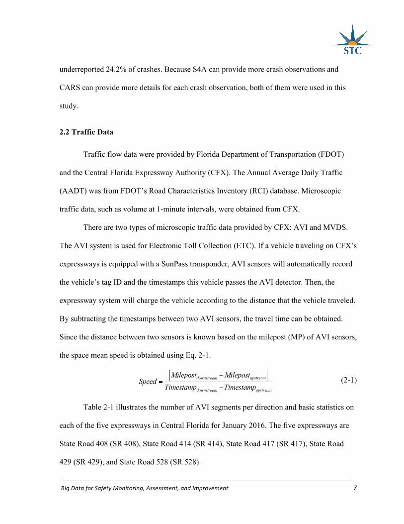
Table 2-1 illustrates the number of AVI segments per direction and basic statistics on
each of the five expressways in Central Florida for January 2016. The five expressways are
State Road 408 (SR 408), State Road 414 (SR 414), State Road 417 (SR 417), State Road
429 (SR 429), and State Road 528 (SR 528).
BigDataforSafetyMonitoring,Assessment,andImprovement 8
Table 2-1 AVI segments on CFX expressway system
Route ID Direction No. of
Segments
Segment Length
Mean Std. Min Max
SR 408 EB 26 0.87 0.47 0.17 1.85
WB 23 0.97 0.53 0.33 2.29
SR 414 EB 5 1.06 0.73 0.29 2.02
WB 4 1.32 0.81 0.35 2.31
SR 417 NB 18 1.84 0.84 0.63 3.98
SB 23 1.42 0.78 0.38 3.10
SR 429 NB 14 1.41 1.08 0.30 4.27
SB 15 2.00 1.20 0.61 4.54
SR 528 EB 8 2.74 2.25 0.33 7.06
WB 8 2.74 2.22 0.86 7.60
Figure 2-1 illustrates the deployment of AVI sensors on the CFX expressway
network. The AVI sensors on SR 408 is the densest, and SR 408 has the smallest mean AVI
segment length of the five expressways in CFX system. The density of AVI sensors are
mainly determined by two aspects: the need for collecting toll and for estimating travel time.
The SR 408 carries the heaviest traffic and travel through the downtown area of Orlando. The
on- and off-ramp density of SR 408 is much higher than other expressways, and AVI sensors
need to put close to on- and off-ramps for toll collection. Additionally, the heavy traffic
produces low travel time reliability and makes the travel time varies a lot for each segment.
Hence, dense AVI sensors are required to more precisely predict travel time.

BigDataforSafetyMonitoring,Assessment,andImprovement 9
Figure 2-1 Deployment of AVI sensors on CFX expressway network
MVDS was introduced to CFX’s expressway system since 2012, and the MVDS data
have been available since July 2013. The system is specifically designed for traffic
monitoring. MVDS detectors were installed at almost every merging and diverging points of
expressway systems. They collect the traffic volume, occupancy, and average speed for each
lane at 1-minute intervals. In addition to the traffic data above, MVDS detectors recognize
the length of passing vehicles and classifies them under four groups:
• Type 1: vehicles 0 to 10 feet in length • Type 2: vehicles 10 to 24 feet in length • Type 3: vehicles 24 to 54 feet in length • Type 4: vehicles over 54 feet in length
There are 364 MVDS detectors along the CFX expressways with an average spacing
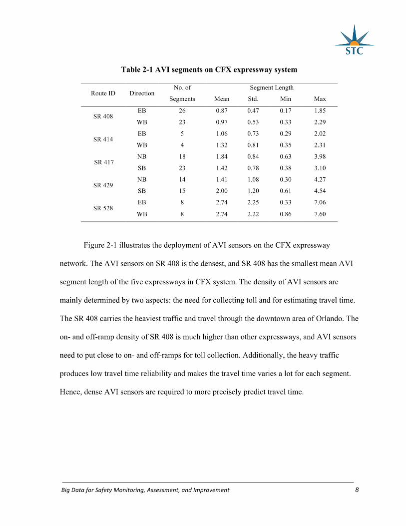
of 0.574 miles. Table 2-2 shows the MVDS detector information for each direction for the
five expressways in January 2016.
Table 2-2 MVDS segments on CFX expressway system
BigDataforSafetyMonitoring,Assessment,andImprovement 10
Route ID Direction No. of
Segments
Segment Length
Mean Std. Min Max
SR 408 EB 56 0.38 0.18 0.10 1.00
WB 53 0.41 0.20 0.10 1.00
SR 414 EB 13 0.44 0.17 0.20 0.70
WB 12 0.46 0.23 0.10 0.90
SR 417 NB 54 0.59 0.29 0.20 1.50
SB 54 0.59 0.29 0.20 1.30
SR 429 NB 28 0.68 0.54 0.20 2.80
SB 28 0.68 0.59 0.10 3.10
SR 528 EB 28 0.84 0.79 0.10 3.00
WB 28 0.84 0.82 0.10 3.10
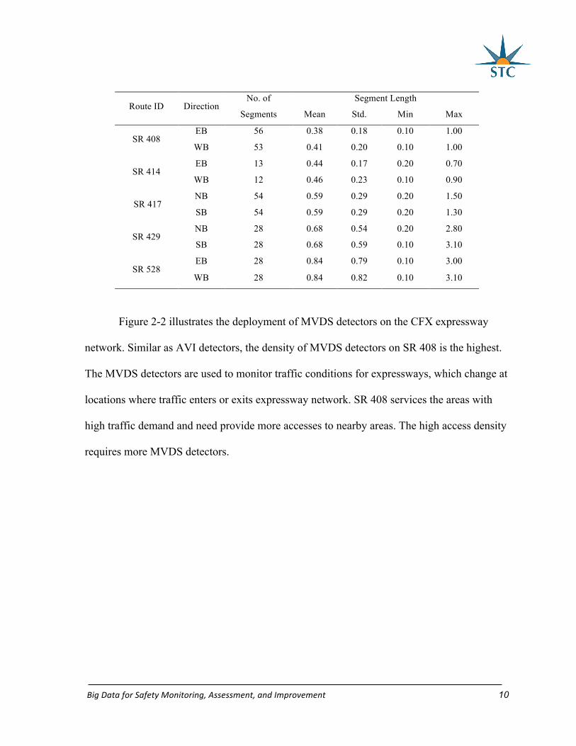
Figure 2-2 illustrates the deployment of MVDS detectors on the CFX expressway
network. Similar as AVI detectors, the density of MVDS detectors on SR 408 is the highest.
The MVDS detectors are used to monitor traffic conditions for expressways, which change at
locations where traffic enters or exits expressway network. SR 408 services the areas with
high traffic demand and need provide more accesses to nearby areas. The high access density
requires more MVDS detectors.
BigDataforSafetyMonitoring,Assessment,andImprovement 11
Figure 2-2 Deployment of MVDS detectors on expressway network
There are much more MVDS detectors than AVI detectors. Comparing Table 2-1 to
Table 2-2, it can be found the number of MVDS detectors is more than twice of AVI sensors
for the majority of directions. Additionally, only part of vehicles equipped SunPass, so AVI
sensors cannot obtain all vehicles’ information. Furthermore, AVI sensors do not distinguish
the lane a vehicle uses and vehicle length, but MVDS detectors are able to provide traffic
data for each lane and recognize vehicle length. Hence, this study more focuses on the
implementation of MVDS traffic data.
2.3 Road Geometric Data
Geometric data were obtained from RCI, which is maintained by FDOT, or manually
collected by using ArcGIS map. The RCI records 323 features and characteristics for the
roadway system (FDOT, 2014). When multiple geometric variables are selected,
homogeneous segments of the roadway were generated automatically. Segments of extreme

BigDataforSafetyMonitoring,Assessment,andImprovement 12
short distance (less than 0.1 mile) were combined with adjacent segment, which shared
higher similarity. The selected geometric characteristics in this study included the number of
lanes, existence of auxiliary lanes, speed limit, horizontal degree of curvature, median width,
and shoulder width. Vertical curves are seldom observed on the expressways because of the
flat terrain in Central Florida and thus were not included. Table 2-3 gives an example on the
RCI data.
Table 2-3 RCI geometric data
RDWYID Begin
milepost
Number of
lanes
Auxiliary
lanes type
Shoulder
width
Median
width
Horizontal
curve
Speed
limit AADT
75008170 1.417 2 10.0 40 0 55 41000
75008170 1.581 2 10.0 40 0 65 41000
75008170 2.206 2 10.0 40 0 65 52500
75008170 2.455 2 10.0 40 0 65 52500
75008170 2.664 2 10.0 40 0 65 52500
75008170 2.903 2 10.0 40 0 65 52500
75008170 3.078 2 10.0 40 0 65 52500
75008170 3.264 2 10.0 40 0.75 65 52500
75008170 3.543 2 10.0 40 0.75 65 52500
75008170 3.717 2 10.0 40 0 65 52500
75008170 3.879 2 10.0 40 1 65 52500
75008170 3.980 3 10.0 40 1 65 52500
75008170 4.242 3 10.0 40 0 65 52500
75008170 4.789 3 10.0 40 2.75 65 52500
75008170 5.027 3 10.0 40 0 65 52500
75008000 0.382 3 10.0 20 1.5 65 46000
75008000 0.640 3 4 10.0 20 1.5 65 46000
75008000 0.725 3 4 10.0 20 0 65 46000
75008000 0.866 3 10.0 20 0 65 46000
BigDataforSafetyMonitoring,Assessment,andImprovement 13
Some geometric information was not provided by RCI, e.g., ramp type (on- or off-
ramp), ramp configuration (loop, diamond, etc.), weaving segment length. Hence, there was a
need to collect these data manually by using ArcGIS map.
2.4 Macroscopic data
The FDOT Central Office periodically develops statewide planning data, network, and
model based on Statewide Traffic Analysis Zones (SWTAZs). The data includes trip
generation variables. The trip generation data include diverse types of trip productions and trip
attractions. A trip production refers to a trip end connected to a residential land-use in a zone
whereas a trip attraction is defined as a trip end connected to a nonresidential land-use in a
zone. For the SWTAZs that the studied ramps are in, total production trips and attractions trips
per day were 5,601 and 5,666, respectively. Such trip production and attraction trips are
provided by trip purposes (i.e., working, social or recreational, shopping, and total). The trip
generation data were processed and converted to percentages by trip purposes. Among the total
trip productions, 15.8% were home-based shopping productions, 14.8% were home-based-
work productions, and 7.1% were home-based social or recreational productions. On the other
hand, among the total trip attractions, 16.4% were home-based-work attractions, 9.3% were
home-based shopping attractions, and 8.4% were home-based social or recreational attractions.
Furthermore, the SWTAZ model also provided land-use variables including population
density, employment density, school enrollment density, and the number of employees by
industry. It was shown that there are averagely about 2,215 residents per square mile (i.e.,
population density), 1,577 employees per square mile, and 902 enrollments per square mile.

BigDataforSafetyMonitoring,Assessment,andImprovement 14
Regarding the percentage of employees by industry type, the percentage of service
employment was the highest (50%), and then is the percentages of retail employment (19.3%).
The macroscopic data for the studied intersections were collected from the American
Community Survey (ACS) of the U.S. Census Bureau. Because multiple spatial units (i.e.,
block group, traffic analysis zone, census tract, ZIP-code tabulation area, traffic analysis
district, census county division, and county) were used in this study, the descriptive statistics
were also provided by these geographic units. It is noteworthy that the basic statistics can be
different by the level of aggregation. For instance, the average population based on block
groups is 2,559; but it is only 631.9 based on counties. This issue is call the Modifiable Areal
Unit Problem (MAUP), which is presented when artificial boundaries are imposed on
continuous geographical surfaces and the aggregation of geographic data cause the variation
in statistical results. The MAUP was observed in the datasets used in this study as there are
more number of zones in the urban area whereas the number of zones is smaller in the rural
area, especially in small zone systems such as block groups, traffic analysis zones, census
tracts, etc. Thus, the average values are more affected by the urban zones in such small zone
systems. The collected variables are as follows: demographic (i.e., population density,
proportions of children, adolescent, middle-age, young elderly, and elderly), transportation
mode (i.e., the proportions of commuters using car, public transit, tax, motorcycle, bicycle,
walking, and other means), socio-economic variables (i.e., the proportion of people working
at home, the school enrollment density, the proportion of people with bachelor’s degree or
higher, the proportion of households below poverty line, the proportion of households with no
vehicle, and median household income). Lastly, the proportion of urbanized area was also
attempted.
BigDataforSafetyMonitoring,Assessment,andImprovement 15
CHAPTER3:PRELIMINARYSAFETYEVALUATION
3.1 Introduction
This chapter carries out visualization of traffic and crash data. Big data are well
known for their huge size, thus, it is usually hard to interpret them without a series of detailed
investigations. Data visualization facilitates researchers’ understanding of the traffic and
crash patterns on the studied subjects. As one of the major expressways in Central Florida
area, SR 408 was chosen as a main study area in this chapter to show the preliminary
analysis. SR 408 travels along east-west direction through Orlando and carries commuting
traffic, especially in morning and evening peak-hours. Both AVI and MVDS data from July
2014 were selected for visualizing traffic-related big data, including spatio-temporal hourly
volume and congestion. Meanwhile, traffic crashes from 2011 to 2014 on all five
expressways were analyzed using crash density visualization.
3.2 Visualization of Spatio-temporal Hourly Volume Distributions
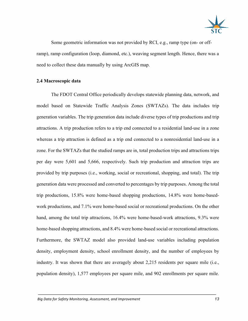
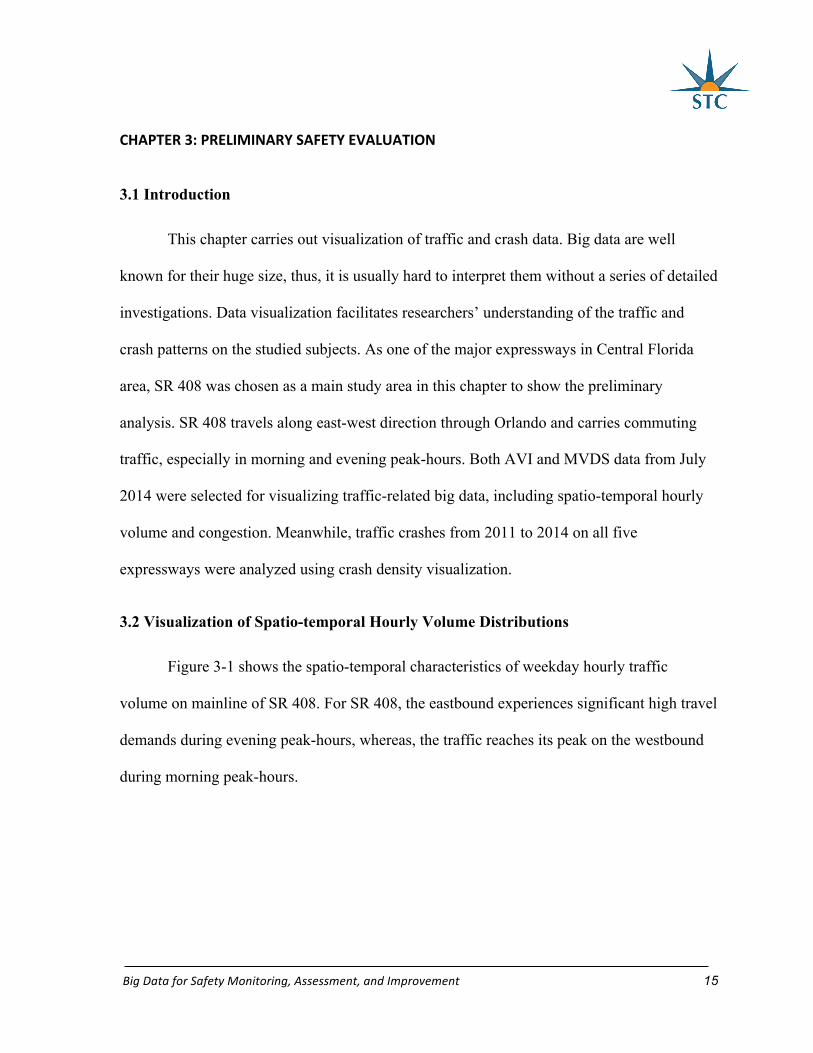
Figure 3-1 shows the spatio-temporal characteristics of weekday hourly traffic
volume on mainline of SR 408. For SR 408, the eastbound experiences significant high travel
demands during evening peak-hours, whereas, the traffic reaches its peak on the westbound
during morning peak-hours.
BigDataforSafetyMonitoring,Assessment,andImprovement 16
(a) Eastbound
(b) Westbound Figure 3-1 Weekday hourly volume along SR 408
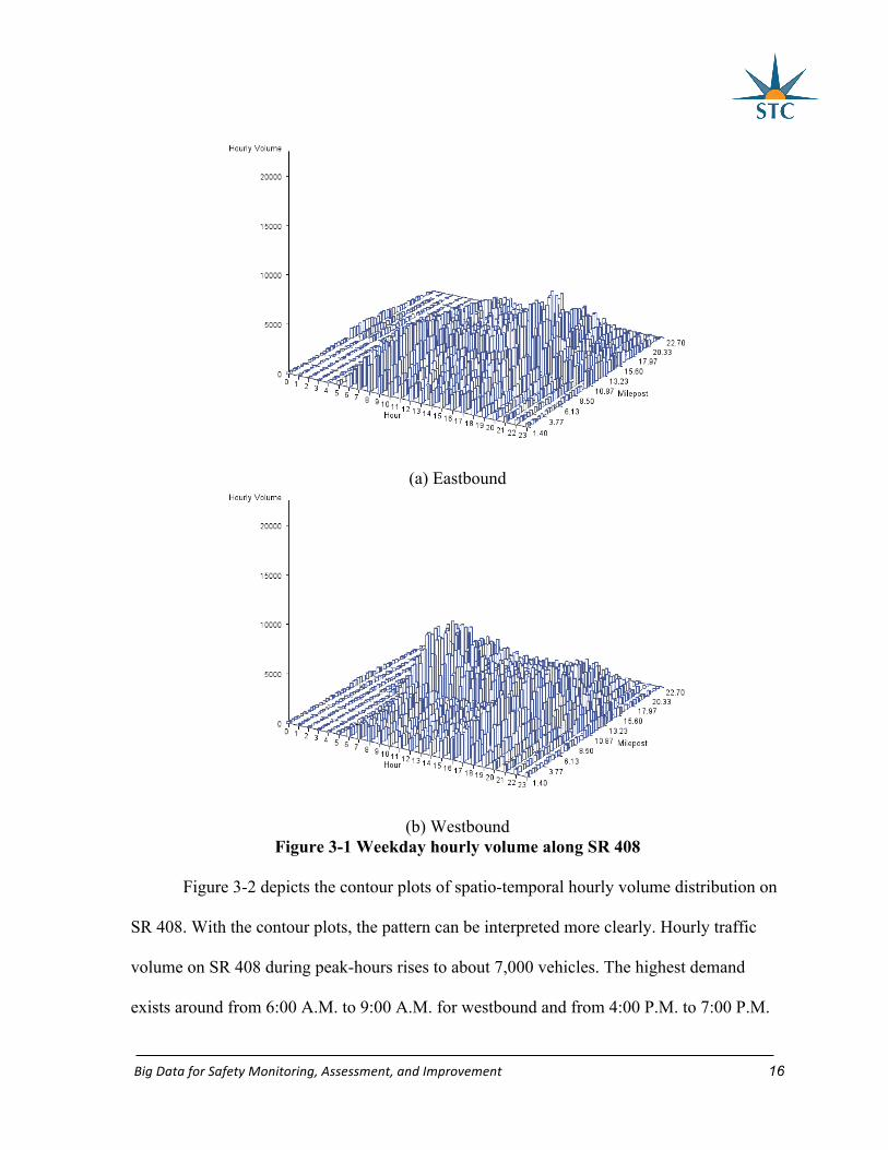
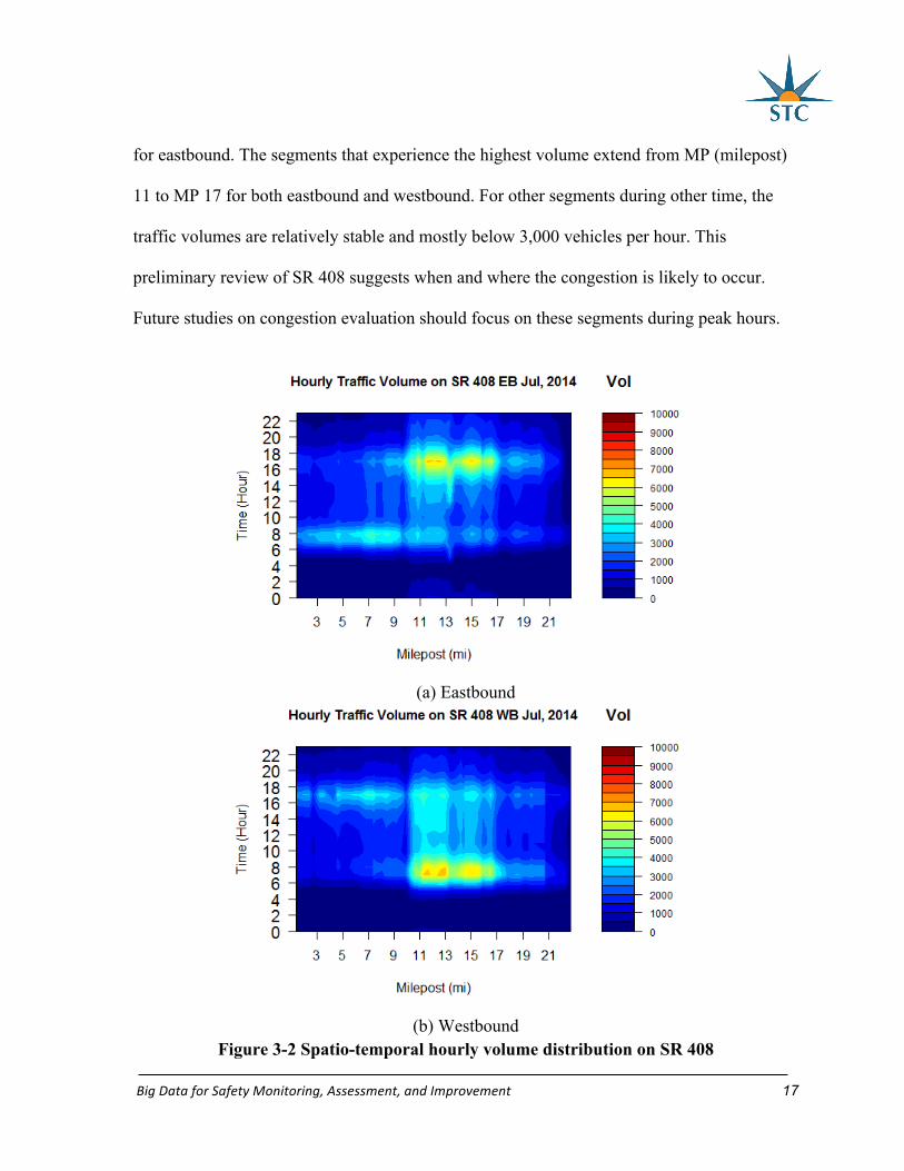
Figure 3-2 depicts the contour plots of spatio-temporal hourly volume distribution on
SR 408. With the contour plots, the pattern can be interpreted more clearly. Hourly traffic
volume on SR 408 during peak-hours rises to about 7,000 vehicles. The highest demand
exists around from 6:00 A.M. to 9:00 A.M. for westbound and from 4:00 P.M. to 7:00 P.M.
BigDataforSafetyMonitoring,Assessment,andImprovement 17
for eastbound. The segments that experience the highest volume extend from MP (milepost)
11 to MP 17 for both eastbound and westbound. For other segments during other time, the
traffic volumes are relatively stable and mostly below 3,000 vehicles per hour. This
preliminary review of SR 408 suggests when and where the congestion is likely to occur.
Future studies on congestion evaluation should focus on these segments during peak hours.
(a) Eastbound
(b) Westbound
Figure 3-2 Spatio-temporal hourly volume distribution on SR 408
BigDataforSafetyMonitoring,Assessment,andImprovement 18
3.3 Visualization of Congestion
Traffic operation on expressways focuses on providing motorists with efficient
movements to their destinations. To achieve this goal, improving congestion is one of the
most important task. Accurate congestion measurement is a prerequisite in congestion
management. Traditionally, volume-to-capacity (V/C) ratios and level of service (LOS) were
implemented by transportation authorities as indicators of congestion intensity (Grant et al.,
2011). Nevertheless, traffic demand can vary considerably in both temporal and spatial
dimensions. Roadway capacity is not fixed, because it might be impacted by crashes,
weather, etc. In such cases, V/C and LOS lack the capability to capture the variability of
congestion. With the fast development of ITS technology, real-time congestion measurement
is becoming an urgent call. On the expressway system, both AVI and MVDS traffic detection
systems are employed. Both of these systems archive the traffic data in real-time manner. In
this project, multiple congestion measures were introduced and compared based on these two
traffic detection systems.
3.3.1 AVI-based Congestion Measurement
Congestion measurement is mainly based on three indexes, namely density, travel
time, and travel speed. AVI system is able to calculate the travel time of vehicles on a
segment. Therefore, congestion measured using travel-time was introduced for the AVI
system. Travel time index (TTI) is a commonly accepted measure used to evaluate traffic
congestion. It is defined as the ratio of actual travel time to an ideal (free-flow) travel time
(Cambridge Systematics, Inc., 2005). The formulation is shown in Eq. 3-1:
TTI = (Actual travel time) / (Free-flow travel time) (3-1)
BigDataforSafetyMonitoring,Assessment,andImprovement 19
It indicates the additional time spent on a trip compared to an ideal trip on the same
corridor. On the Central Florida expressway system, free flow travel time for each segment is
in the AVI traffic data. Free-flow travel time is calculated based on segment length and its
speed limit. If a segment has more than one speed limit, then the average speed limit is used.
According to a study by Griffin (2011), the levels of congestion and the corresponding travel
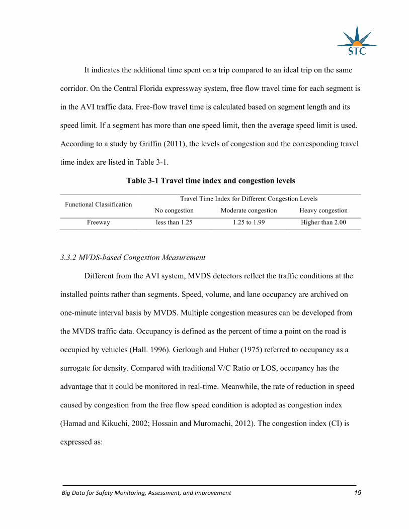
time index are listed in Table 3-1.
Table 3-1 Travel time index and congestion levels
Functional Classification Travel Time Index for Different Congestion Levels
No congestion Moderate congestion Heavy congestion
Freeway less than 1.25 1.25 to 1.99 Higher than 2.00
3.3.2 MVDS-based Congestion Measurement
Different from the AVI system, MVDS detectors reflect the traffic conditions at the
installed points rather than segments. Speed, volume, and lane occupancy are archived on
one-minute interval basis by MVDS. Multiple congestion measures can be developed from
the MVDS traffic data. Occupancy is defined as the percent of time a point on the road is
occupied by vehicles (Hall. 1996). Gerlough and Huber (1975) referred to occupancy as a
surrogate for density. Compared with traditional V/C Ratio or LOS, occupancy has the
advantage that it could be monitored in real-time. Meanwhile, the rate of reduction in speed
caused by congestion from the free flow speed condition is adopted as congestion index
(Hamad and Kikuchi, 2002; Hossain and Muromachi, 2012). The congestion index (CI) is
expressed as:

BigDataforSafetyMonitoring,Assessment,andImprovement 20
( ) / ( ) 00 0free flow speed Actual speed free flow speed When CI
CIWhen CI
− − − >⎧= ⎨
≤⎩ (3-2)
The CI is a continuous congestion indicator ranging from zero to one. The free flow
speed is the 85th percentile speed at the studied location for the whole study period. From Eq.
3-2 above, it can be seen that when the actual speed is above free flow speed, CI will be
recorded as zero. When CI increases, the congestion becomes more severe.
Currently, for the congestion measures calculated from MVDS data, there is no
specific relationship between occupancy or CI and level of congestion is available. However,
the TTI value of 1.25 and 2 are approximately equivalent to CI value of 0.2 and 0.5.
According to the congestion plots, when CI reaches 0.2 and 0.5, the corresponding
occupancy (%) is about 15 and 25. Therefore, congestion levels defined by occupancy and CI
as displayed in Table 3-2 (Shi, 2014). Nevertheless, further refinement of these thresholds
might be possible.
Table 3-2 MVDS-based congestion index and congestion levels
Congestion measure Travel Time Index for Different Congestion Levels
No congestion Moderate congestion Heavy congestion
Occupancy (%) ≤ 15 15 – 24.99 ≥ 25
CI ≤ 0.2 0.2 – 0.499 ≥ 0.5
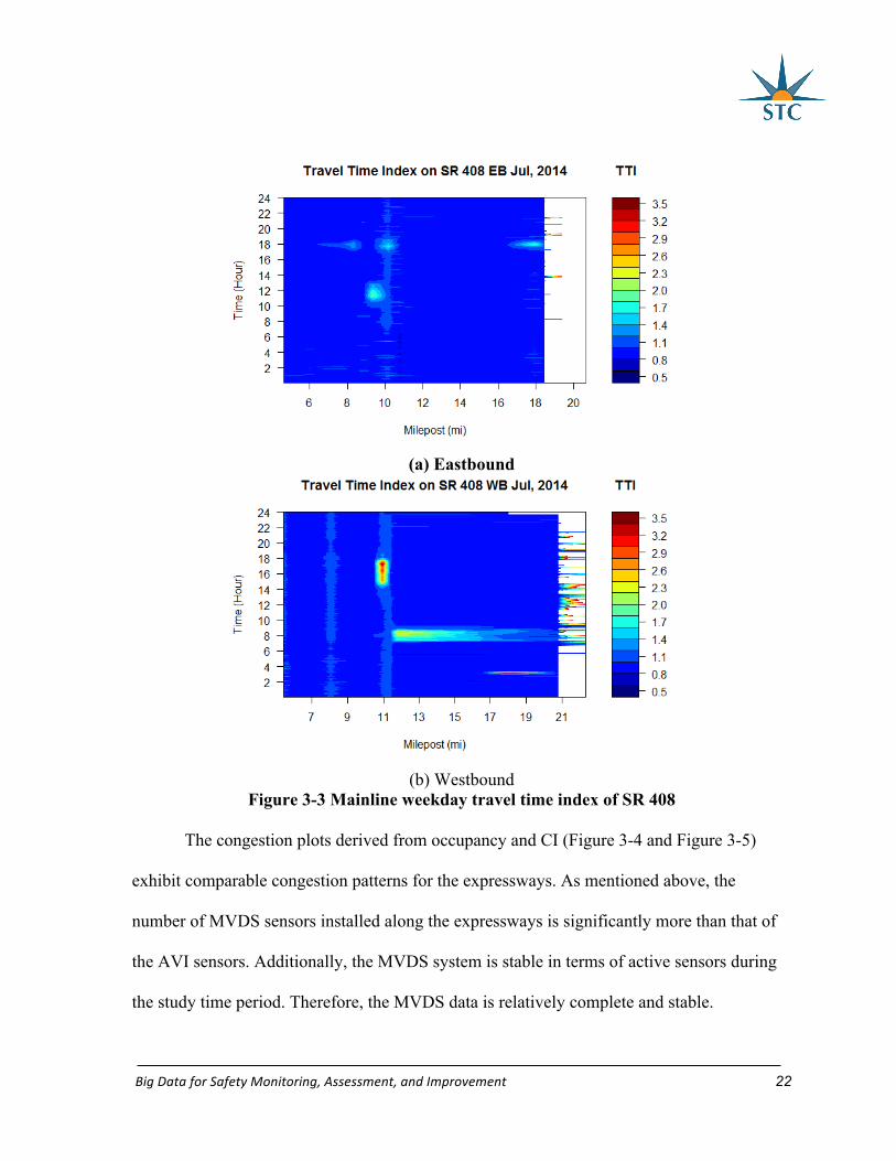
3.3.3 Expressway Mainline Congestion
To measure expressway mainline congestion conditions, the traffic data were
aggregated at five-minute interval and were averaged by the weekdays for July 2014.
Contour plots were generated to illustrate the spatio-temporal property of the congestion. The
TTI congestion plots shown in Figure 3-3 illustrate a proportion of AVI data near MP 20
BigDataforSafetyMonitoring,Assessment,andImprovement 21
were missing for both directions in July 2014, because those sensors in that month were
under maintenance. Despite the incompleteness of AVI data, some patterns could be found
from Figure 3-3, on SR 408 eastbound, congestion is found near MP 9.0 and MP 18.0 in the
evening peak hours. On SR 408 westbound, morning congestion is observed from MP 11.0 to
MP 15.0. These congestion patterns could also be found in Figure 3-4 and Figure 3-5,
indicating that AVI data could reflect congestion to certain extent. However, it is still
important to have complete data to evaluate the performance of AVI-based congestion
measure.
BigDataforSafetyMonitoring,Assessment,andImprovement 22
(a) Eastbound
(b) Westbound
Figure 3-3 Mainline weekday travel time index of SR 408
The congestion plots derived from occupancy and CI (Figure 3-4 and Figure 3-5)
exhibit comparable congestion patterns for the expressways. As mentioned above, the
number of MVDS sensors installed along the expressways is significantly more than that of
the AVI sensors. Additionally, the MVDS system is stable in terms of active sensors during
the study time period. Therefore, the MVDS data is relatively complete and stable.
BigDataforSafetyMonitoring,Assessment,andImprovement 23
(a) Eastbound
(b) Westbound
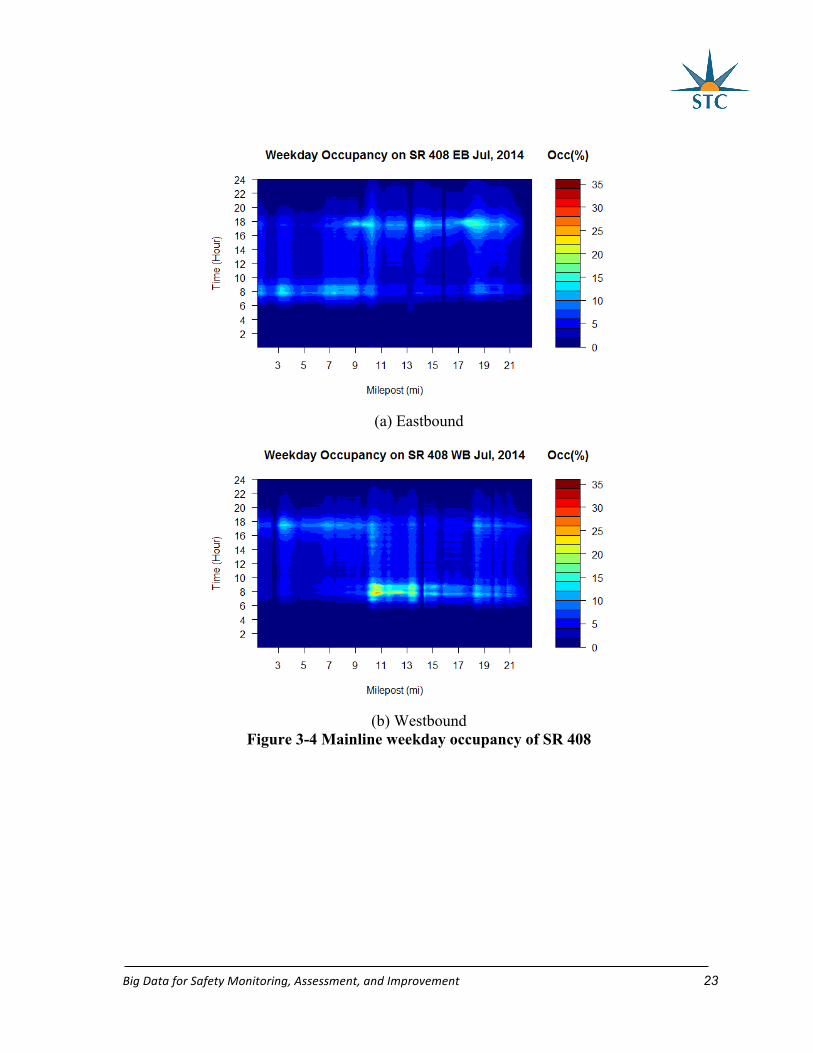
Figure 3-4 Mainline weekday occupancy of SR 408
BigDataforSafetyMonitoring,Assessment,andImprovement 24
(a) Eastbound
(b) Westbound
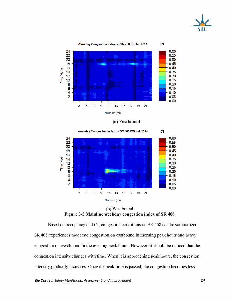
Figure 3-5 Mainline weekday congestion index of SR 408
Based on occupancy and CI, congestion conditions on SR 408 can be summarized.
SR 408 experiences moderate congestion on eastbound in morning peak hours and heavy
congestion on westbound in the evening peak hours. However, it should be noticed that the
congestion intensity changes with time. When it is approaching peak hours, the congestion
intensity gradually increases. Once the peak time is passed, the congestion becomes less
BigDataforSafetyMonitoring,Assessment,andImprovement 25
severe. The congested area for SR 408 is approximately from MP 17.0 to MP 19.0 on
eastbound and from MP 10.0 to MP 13.0 on westbound.
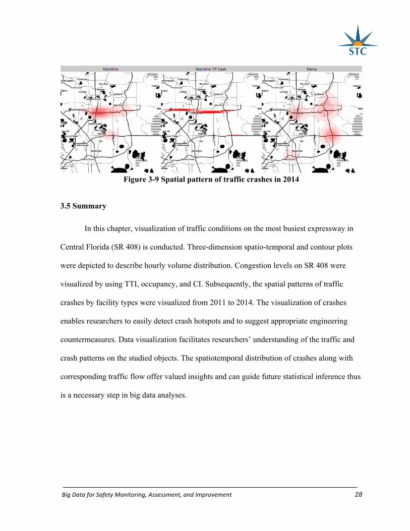
3.4 Visualization of Crashes on Expressways
For the total crashes on the expressway system, the spatial pattern of crashes is
examined through crash density. The spatial distribution of crashes on mainlines and ramps
can be found in Figures 3-6 to 3-9. Toll plazas in Central Florida expressway system have
two types of lane: express lane and cash lane. Vehicles on expressway lanes use ETC to pay
toll fee automatically, but those on cash lane need to stop at tollbooth to pay toll. Hence, the
driver behaviors on toll plaza cash lane are different from other mainlines, and the crash
pattern of cash lane was explored separately.
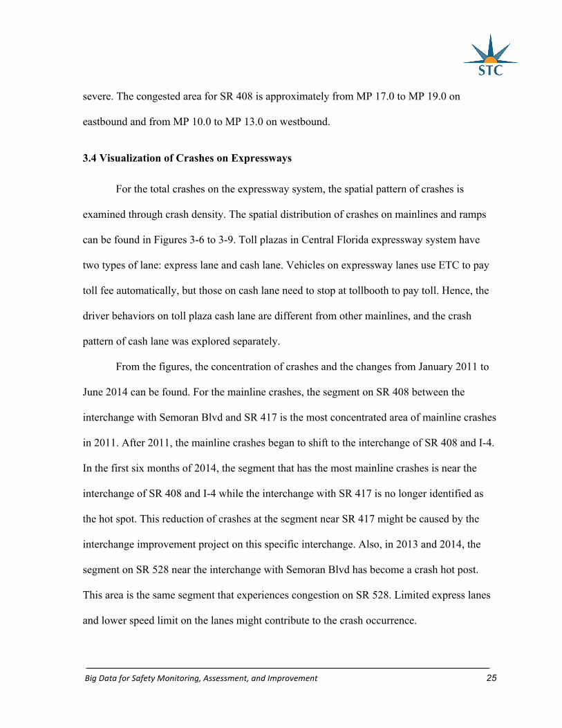
From the figures, the concentration of crashes and the changes from January 2011 to
June 2014 can be found. For the mainline crashes, the segment on SR 408 between the
interchange with Semoran Blvd and SR 417 is the most concentrated area of mainline crashes
in 2011. After 2011, the mainline crashes began to shift to the interchange of SR 408 and I-4.
In the first six months of 2014, the segment that has the most mainline crashes is near the
interchange of SR 408 and I-4 while the interchange with SR 417 is no longer identified as
the hot spot. This reduction of crashes at the segment near SR 417 might be caused by the
interchange improvement project on this specific interchange. Also, in 2013 and 2014, the
segment on SR 528 near the interchange with Semoran Blvd has become a crash hot post.
This area is the same segment that experiences congestion on SR 528. Limited express lanes
and lower speed limit on the lanes might contribute to the crash occurrence.

BigDataforSafetyMonitoring,Assessment,andImprovement 26
The number of crashes on mainline toll plaza cash lanes is relatively small compared
with those of mainline and ramp crashes. The low number of cash lane crashes result in
significant crash pattern change even though a small variation of crash counts. Hence, crash
hot spots for toll plaza cash lanes were not fixed in these years. Nevertheless, Pine Hills
Mainline Toll Plaza, Conway Road Mainline Toll Plaza on SR 408, John Young Parkway
Mainline Toll Plaza, University Mainline Toll Plaza on SR 417, and Beachline Mainline Toll
Plaza on SR 528 were found to be the toll plazas on the mainline that can have more crashes
on their cash lanes.
For the ramp crashes, the similar pattern as mainline crashes on SR 408 were also
detected. From 2011 to 2013, ramps at the interchange between SR 408 and SR 417 had the
highest crash density. However, this pattern changed in 2014 as that the interchange between
SR 408 and I-4 becomes the concentration area of ramp crashes on SR 408. The interchange
between SR 417 and SR 528 is also a major area for ramp crashes. Also, the ramps on SR
417 at John Young Parkway and Orange Blossom Trail were found to be more likely to have
ramp crashes. The findings of mainline crashes, mainline toll plaza cash lane crashes, and
ramp crashes shows the concentrated locations of each type of these crashes. The changes in
crash density on the expressway system are found. The results can be used for potential
safety improvement projects in the future.
BigDataforSafetyMonitoring,Assessment,andImprovement 27
Figure 3-6 Spatial pattern of traffic crashes in 2011
Figure 3-7 Spatial pattern of traffic crashes in 2012
Figure 3-8 Spatial pattern of traffic crashes in 2013
BigDataforSafetyMonitoring,Assessment,andImprovement 28
Figure 3-9 Spatial pattern of traffic crashes in 2014
3.5 Summary
In this chapter, visualization of traffic conditions on the most busiest expressway in
Central Florida (SR 408) is conducted. Three-dimension spatio-temporal and contour plots
were depicted to describe hourly volume distribution. Congestion levels on SR 408 were
visualized by using TTI, occupancy, and CI. Subsequently, the spatial patterns of traffic
crashes by facility types were visualized from 2011 to 2014. The visualization of crashes
enables researchers to easily detect crash hotspots and to suggest appropriate engineering
countermeasures. Data visualization facilitates researchers’ understanding of the traffic and
crash patterns on the studied objects. The spatiotemporal distribution of crashes along with
corresponding traffic flow offer valued insights and can guide future statistical inference thus
is a necessary step in big data analyses.
BigDataforSafetyMonitoring,Assessment,andImprovement 29
CHAPTER4:REAL-TIMECONFLICTPRECURSORSFORWEAVINGSEGMENTS
4.1 Introduction
Traditional traffic safety studies are mainly based on historic traffic crash data.
However, the usage of crash data is sometimes limited because of the unreliability of crash
records and the long time needed to collect adequate crash samples (Glennon and Thorson,
1975; Essa and Sayed, 2015). Therefore, there has been plenty of traffic safety studies, which
rely on surrogate safety measures.
One of the most commonly used surrogate measures is traffic conflicts. A traffic
conflict was defined as a traffic event involving two or more road users, in which one user
performs some unusual actions, such as a change in direction or speed, these unusual actions
place another user in the danger of a collision unless an evasive maneuver is undertaken
(Migletz et al., 1985). Previous studies have proven that conflict counts are positively related
to crash counts, and the relationship is statistically significant (Meng and Qu, 2012; Sacchi
and Sayed, 2016). Furthermore, researchers collected field conflict counts on roadway
facilities to uncover potential safety hazard (Van Der Horst et al., 2014), and to verify the
safety impacts of countermeasures, such as raised crosswalks (Cafiso et al., 2011; Autey et
al., 2012). However, the majority of previous studies only focused on conflict count, but
were not interested in the cause of each conflict and did not analyze conflicts from a
microscopic aspect.
One of the studies that explore traffic safety from a microscopic aspect is real-time
safety analysis. The real-time safety analysis intends to identify precursors that are relatively
more “hazard prone” that other parameters. It is accomplished by comparing and analyzing
BigDataforSafetyMonitoring,Assessment,andImprovement 30
traffic, weather, and other conditions right before the occurrence of hazard and non-hazard
events, and furthermore by estimating the likelihood of hazard events. The hazard events
include crash and conflict events. The real-time crash analysis research has been successfully
done by plenty of previous studies (Zheng et al., 2010; Yu and Abdel-Aty, 2013a). However,
there has not been enough real-time conflict analyses.
This chapter implements microscopic simulation and Surrogate Safety Assessment
Model (SSAM) to conduct real-time conflict study. To build a well-calibrated and validated
simulation network, this study first adopted high-resolution big traffic data from MVDS to
serve as the traffic volume input and desired speed distribution input. Meanwhile, the
microscopic simulation network were built based on a two level calibration and validation
method. The method is able to enhance the consistency between simulated safety and filed
safety, and between simulated traffic and field traffic. In simulation, conflicts are identified
by SSAM, a software developed by Federal Highway Administration (FHWA). The SSAM
automatically conducts conflict analysis by directly processing vehicle trajectory data from
simulation output. The conflict analysis contains conflict location, time, type, etc. After
obtaining time and location of a conflict or non-conflict event, the event is matched with the
traffic data just before it. Then a logistic regression models are employed to distinguish
conflict events from non-conflict events using traffic parameters.
4.2 Experiment Design
4.2.1 VISSIM Network Building
One of the most important parts of this chapter is building a calibrated and validated
VISSIM network. Previous studies on weaving segments’ microscopic simulation only

BigDataforSafetyMonitoring,Assessment,andImprovement 31
compared simulated traffic with field traffic (Wu et al., 2005; Jolovic and Stevanovic, 2013).
The results showed that the simulated traffic was consistent with field traffic if driver
behavior parameters in the simulation were adjusted. However, this chapter focuses on real-
time conflict analysis in microscopic simulation. Hence, not only traffic condition in
simulation needs to be calibrated and validated, but also safety condition of the simulation
network requires validation.
In order to ensure both traffic and safety of the simulation network are consistent with
those of the field, a two level calibration and validation method was used. At the first level,
the traffic conditions of weaving segments were calibrated and validated based on field
MVDS data. At the second level, the simulated conflict count of each weaving segment was
compared to its crash frequency. If the simulated speed or conflict is not consistent with its
corresponding field value, driver behavior parameters need to be adjusted. The calibration
and validation procedure is shown in Figure 4-1.
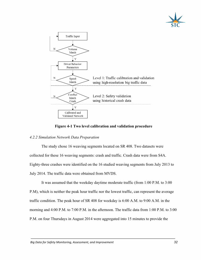
BigDataforSafetyMonitoring,Assessment,andImprovement 32
Figure 4-1 Two level calibration and validation procedure
4.2.2 Simulation Network Data Preparation
The study chose 16 weaving segments located on SR 408. Two datasets were
collected for these 16 weaving segments: crash and traffic. Crash data were from S4A.
Eighty-three crashes were identified on the 16 studied weaving segments from July 2013 to
July 2014. The traffic data were obtained from MVDS.
It was assumed that the weekday daytime moderate traffic (from 1:00 P.M. to 3:00
P.M), which is neither the peak hour traffic nor the lowest traffic, can represent the average
traffic condition. The peak hour of SR 408 for weekday is 6:00 A.M. to 9:00 A.M. in the
morning and 4:00 P.M. to 7:00 P.M. in the afternoon. The traffic data from 1:00 P.M. to 3:00
P.M. on four Thursdays in August 2014 were aggregated into 15 minutes to provide the

BigDataforSafetyMonitoring,Assessment,andImprovement 33
VISSIM traffic input, including volume and Heavy Goods Vehicles (HGVs) percentage. The
Type 3 and Type 4 vehicles in MVDS data were considered as HGVs in VISSIM.
Desired speed distribution is also an important input for the VISSIM network. If not
hindered by other vehicles or network objects, e.g. signal controls, a driver will travel at
his/her desired speed (PTV, 2013). The speed data during 11:00 A.M. to 1:00 P.M. on
Thursdays in August 2014 were chosen. During this period, the traffic volume is the lowest
in the daytime. Thus, the possibility of a vehicle constrained by other vehicles is low and
vehicles are more likely to travel at their desired speed. Generally, the desired speed
distribution is decided by geometric design, e.g., degree of curvature, speed limit. The
desired speed distribution for each location might not be the same. Hence, this study divided
the locations of SR 408 into seven groups according to the similarity of speed limit and field
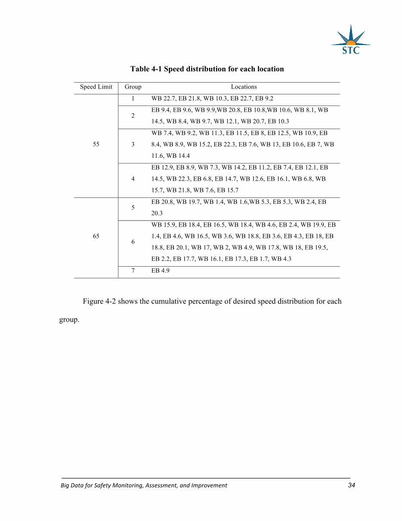
speed distribution of each location. The group information is in Table 4-1. In the table, for
each location, the beginning two letters stand for direction, i.e., WB is westbound and EB is
eastbound; the numbers stand for milepost.
BigDataforSafetyMonitoring,Assessment,andImprovement 34
Table 4-1 Speed distribution for each location
Speed Limit Group Locations
55
1 WB 22.7, EB 21.8, WB 10.3, EB 22.7, EB 9.2
2 EB 9.4, EB 9.6, WB 9.9,WB 20.8, EB 10.8,WB 10.6, WB 8.1, WB
14.5, WB 8.4, WB 9.7, WB 12.1, WB 20.7, EB 10.3
3
WB 7.4, WB 9.2, WB 11.3, EB 11.5, EB 8, EB 12.5, WB 10.9, EB
8.4, WB 8.9, WB 15.2, EB 22.3, EB 7.6, WB 13, EB 10.6, EB 7, WB
11.6, WB 14.4
4
EB 12.9, EB 8.9, WB 7.3, WB 14.2, EB 11.2, EB 7.4, EB 12.1, EB
14.5, WB 22.3, EB 6.8, EB 14.7, WB 12.6, EB 16.1, WB 6.8, WB
15.7, WB 21.8, WB 7.6, EB 15.7
65
5 EB 20.8, WB 19.7, WB 1.4, WB 1.6,WB 5.3, EB 5.3, WB 2.4, EB
20.3
6
WB 15.9, EB 18.4, EB 16.5, WB 18.4, WB 4.6, EB 2.4, WB 19.9, EB
1.4, EB 4.6, WB 16.5, WB 3.6, WB 18.8, EB 3.6, EB 4.3, EB 18, EB
18.8, EB 20.1, WB 17, WB 2, WB 4.9, WB 17.8, WB 18, EB 19.5,
EB 2.2, EB 17.7, WB 16.1, EB 17.3, EB 1.7, WB 4.3
7 EB 4.9
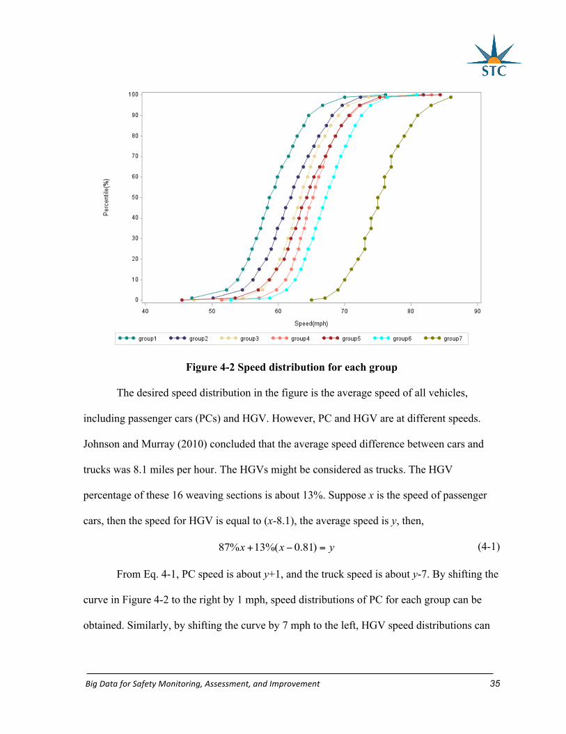
Figure 4-2 shows the cumulative percentage of desired speed distribution for each
group.
BigDataforSafetyMonitoring,Assessment,andImprovement 35
Figure 4-2 Speed distribution for each group
The desired speed distribution in the figure is the average speed of all vehicles,
including passenger cars (PCs) and HGV. However, PC and HGV are at different speeds.
Johnson and Murray (2010) concluded that the average speed difference between cars and
trucks was 8.1 miles per hour. The HGVs might be considered as trucks. The HGV
percentage of these 16 weaving sections is about 13%. Suppose x is the speed of passenger
cars, then the speed for HGV is equal to (x-8.1), the average speed is y, then,
87% 13%( 0.81)x x y+ − = (4-1)
From Eq. 4-1, PC speed is about y+1, and the truck speed is about y-7. By shifting the
curve in Figure 4-2 to the right by 1 mph, speed distributions of PC for each group can be
obtained. Similarly, by shifting the curve by 7 mph to the left, HGV speed distributions can
BigDataforSafetyMonitoring,Assessment,andImprovement 36
be gained. Finally, there are 14 desired speed distributions, among which seven are for PCs
and seven for HGVs.
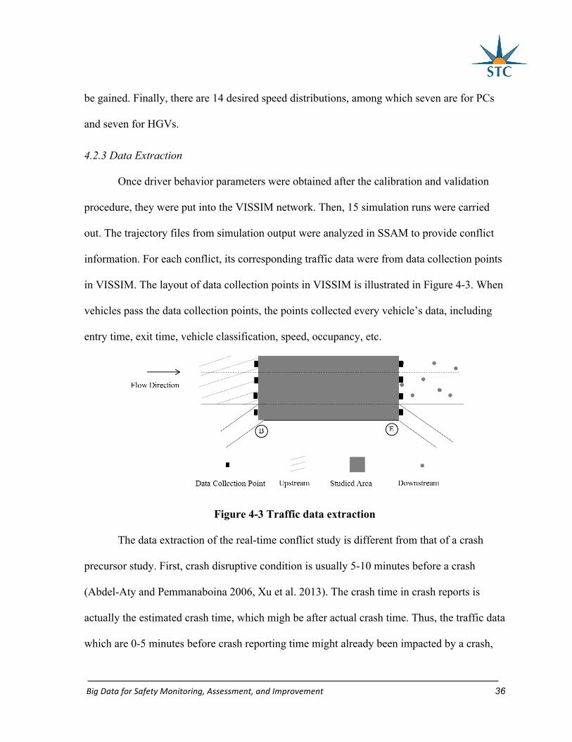
4.2.3 Data Extraction
Once driver behavior parameters were obtained after the calibration and validation
procedure, they were put into the VISSIM network. Then, 15 simulation runs were carried
out. The trajectory files from simulation output were analyzed in SSAM to provide conflict
information. For each conflict, its corresponding traffic data were from data collection points
in VISSIM. The layout of data collection points in VISSIM is illustrated in Figure 4-3. When
vehicles pass the data collection points, the points collected every vehicle’s data, including
entry time, exit time, vehicle classification, speed, occupancy, etc.
Figure 4-3 Traffic data extraction
The data extraction of the real-time conflict study is different from that of a crash
precursor study. First, crash disruptive condition is usually 5-10 minutes before a crash
(Abdel-Aty and Pemmanaboina 2006, Xu et al. 2013). The crash time in crash reports is
actually the estimated crash time, which migh be after actual crash time. Thus, the traffic data
which are 0-5 minutes before crash reporting time might already been impacted by a crash,

BigDataforSafetyMonitoring,Assessment,andImprovement 37
so the trafific data 5-10 minutes before the time in crash report are usually chosen. However,
for the conflict precursor study, the accurate conflict time can be obtained from SSAM.
Hence, the traffic data, which are 0-5 minutes before a conflict, were chosen as conflict
disruptive events. As for the non-disruptive events, they were 5-minute interval traffic data
and were defined as the conditions, which neither resulted in a conflict nor were under
influence of conflicts. In this study, it was assumed that traffic conditions were not impacted
by conflicts if they were more than 60 seconds after conflicts, because conflicts are cleared
quickly in simulation and the influence of conflicts on traffic vanish soon. Furthermore, in
order to explore conflict mechanisms more closely, the study also adopted the traffic data
that were 0-1 minutes before conflicts as disruptive condition, and the non-disruptive traffic
data were also at 1-minute intervals. Hence, two datasets were prepared: one was based on 5-
minute interval; the other one was based on 1-minute interval.
Second, in crash prediction studies, the number of non-disruptive conditions is much
more than that of disruptive conditions. In order to balance the sample size of disruptive and
non-disruptive conditions, non-disruptive condition observations are randomly selected from
the full samples (Abdel-Aty et al. 2004, Hossain and Muromachi 2010, Xu et al. 2013).
Nevertheless, conflict number is much more than crash number. Gettman et al. (2008) found
that the probability of being involved in a crash given a traffic conflict is 0.005% at
intersections. This indicates that the conflict number was 20,000 times of the crash number in
their study. In real-time conflict study, the sample size of disruptive conflict condition is
largely enriched, and the sample size of non-disruptive conflict condition is significantly
decreased. There was no need to select randomly the non-disruptive conflict condition
samples.
BigDataforSafetyMonitoring,Assessment,andImprovement 38
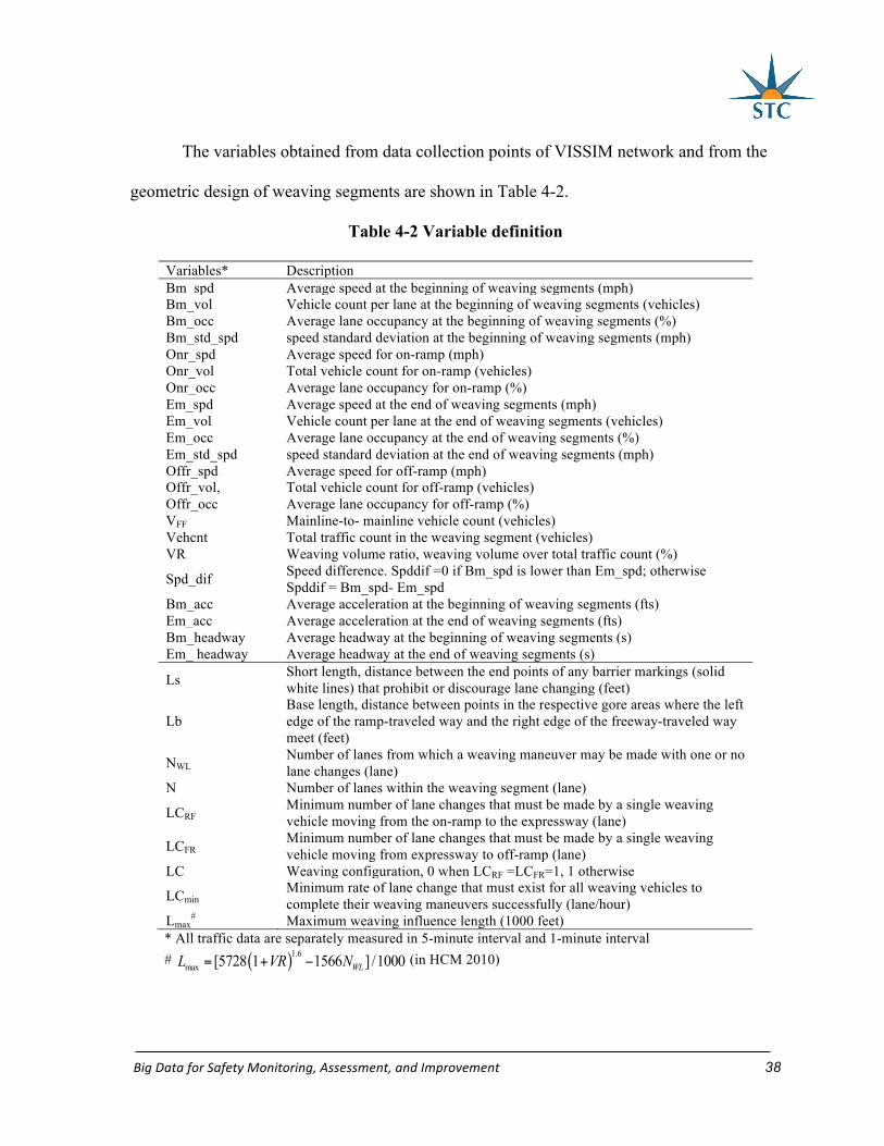
The variables obtained from data collection points of VISSIM network and from the
geometric design of weaving segments are shown in Table 4-2.
Table 4-2 Variable definition
Variables* Description Bm_spd Average speed at the beginning of weaving segments (mph) Bm_vol Vehicle count per lane at the beginning of weaving segments (vehicles) Bm_occ Average lane occupancy at the beginning of weaving segments (%) Bm_std_spd speed standard deviation at the beginning of weaving segments (mph) Onr_spd Average speed for on-ramp (mph) Onr_vol Total vehicle count for on-ramp (vehicles) Onr_occ Average lane occupancy for on-ramp (%) Em_spd Average speed at the end of weaving segments (mph) Em_vol Vehicle count per lane at the end of weaving segments (vehicles) Em_occ Average lane occupancy at the end of weaving segments (%) Em_std_spd speed standard deviation at the end of weaving segments (mph) Offr_spd Average speed for off-ramp (mph) Offr_vol, Total vehicle count for off-ramp (vehicles) Offr_occ Average lane occupancy for off-ramp (%) VFF Mainline-to- mainline vehicle count (vehicles) Vehcnt Total traffic count in the weaving segment (vehicles) VR Weaving volume ratio, weaving volume over total traffic count (%)
Spd_dif Speed difference. Spddif =0 if Bm_spd is lower than Em_spd; otherwise Spddif = Bm_spd- Em_spd
Bm_acc Average acceleration at the beginning of weaving segments (fts) Em_acc Average acceleration at the end of weaving segments (fts) Bm_headway Average headway at the beginning of weaving segments (s) Em_ headway Average headway at the end of weaving segments (s)
Ls Short length, distance between the end points of any barrier markings (solid white lines) that prohibit or discourage lane changing (feet)
Lb Base length, distance between points in the respective gore areas where the left edge of the ramp-traveled way and the right edge of the freeway-traveled way meet (feet)
NWL Number of lanes from which a weaving maneuver may be made with one or no lane changes (lane)
N Number of lanes within the weaving segment (lane)
LCRF Minimum number of lane changes that must be made by a single weaving vehicle moving from the on-ramp to the expressway (lane)
LCFR Minimum number of lane changes that must be made by a single weaving vehicle moving from expressway to off-ramp (lane)
LC Weaving configuration, 0 when LCRF =LCFR=1, 1 otherwise
LCmin Minimum rate of lane change that must exist for all weaving vehicles to complete their weaving maneuvers successfully (lane/hour)
Lmax# Maximum weaving influence length (1000 feet)
* All traffic data are separately measured in 5-minute interval and 1-minute interval # ( )1.6max [5728 1 1566 ] /1000WLL VR N= + − (in HCM 2010)
BigDataforSafetyMonitoring,Assessment,andImprovement 39
4.3 VISSIM Network Calibration and Validation
Based on the previous literatures (Koppula, 2002; Wu et al., 2005; Woody, 2006;
Jolovic and Stevanovic, 2013), four parameters were chosen for VISSIM calibration and
validation. They were desired lane change distance (DLCD), stand still distance (CC0),
following headway time (CC1), and following variation (CC2). DLCD defines the distance at
which vehicles begin to attempt to change lanes in order to arrive at their desinations. CC0 is
desired distance between stopped vehicles. CC1 is following headway time, which means the
time (in seconds) a driver wants to keep. The higher the CC1, the more cautious the driver is.
CC2 is following variation, which restricts the longitudinal oscillation or how much more
distance than the desired safety distance a driver allows before he/she intentionally moves
closer to the car in front (PTV group, 2013).
The study first used the recommended parameters’ value from previous studies to
validate the VISSIM network (Koppula, 2002; Wu et al., 2005; Woody, 2006; Jolovic and
Stevanovic, 2013). The results showed the previous studies’ conclusions were valid only
when traffic was compared. However, when comparing the simulated conflict counts with the
field crash frequencies, the correlation coefficients were not significant. This is because the
parameters’ values were gained without considering the safety in previous studies.
There was a need to revalidate the weaving segment VISSIM network with respect to
both traffic and safety. Twenty-three sets of parameters were tried and each set was run three
times with different random seeds. After excluding 30 minutes VISSIM warm up time and 30
minutes cool down time, 60 minutes VISSIM data were put into use. For the 16 weaving
segments network, the results showed that VISSIM could provide good traffic and safety
BigDataforSafetyMonitoring,Assessment,andImprovement 40
results when the DLCD was 300 meters, CC0 was 1.5 meters, CC1 was 1.5 seconds, and
CC2 was 4 meters. 15 more runs using the parameters above were carried out. For the 15
simulation runs, the average GEH value of the validated VISSIM network was 1.82, and
96.0% of GEH were less than 5 for a 15 minutes interval. As for the speed, the average
absolute of speed difference was 2.00 mph, and 92.2% of speed differences were less than 5
mph for a 5 minutes interval. The good results also implied that implementing big traffic data
can help in build microscopic simulation networks with good quality. The results approved
that the traffic calibration and validation satisfy the requirements, and indicate the traffic on
the weaving segment network was consistent with that of the field (Nezamuddin et al., 2011;
Yu and Abdel-Aty, 2014).
After the traffic calibration and validation, the trajectory files of the simulation runs
were processed in SSAM. Several conflict measurements can be obtained from SSAM, such
as time-to-collision (TTC) and post-encroachment-time (PET). TTC is defined as the
expected time for two vehicles to collide if they remain at their present speed and continue on
their respective trajectories; PET is time difference between the arrivals of two vehicles at the
potential point of collision (Gettman and Head, 2003). In this study, a conflict was identified
when TTC was less than 1.5 seconds and PET was less than 5.0 seconds. The same
thresholds were also widely adopted by other studies (Stevanovic et al., 2013; Saleem et al.,
2014; Saulino et al., 2015). Meanwhile, when TTC was 0, the observation was deleted
(Gettman et al., 2008).
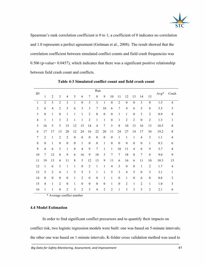
The average simulated conflict count for each weaving segment was then compared
with the corresponding crash frequency. The information can be found in Table 4-3. Then,
SAS procedure ‘Corr’ was used to conduct a Spearman rank correlation test. The range of
BigDataforSafetyMonitoring,Assessment,andImprovement 41
Spearman’s rank correlation coefficient is 0 to 1; a coefficient of 0 indicates no correlation
and 1.0 represents a perfect agreement (Gettman et al., 2008). The result showed that the
correlation coefficient between simulated conflict counts and field crash frequencies was
0.506 (p-value= 0.0457), which indicates that there was a significant positive relationship
between field crash count and conflicts.
Table 4-3 Simulated conflict count and field crash count
ID Run
Avg* Crash 1 2 3 4 5 6 7 8 9 10 11 12 13 14 15
1 2 3 2 3 1 0 3 3 1 0 2 0 0 3 0 1.5 4
2 6 4 2 5 6 3 3 7 10 6 7 4 6 5 8 5.5 3
3 0 1 0 1 1 1 2 0 0 0 1 1 0 3 2 0.9 4
4 1 1 3 2 1 1 2 1 1 0 1 2 2 0 2 1.3 1
5 16 5 5 15 12 15 14 4 7 5 8 10 13 16 13 10.5 8
6 17 17 13 20 12 24 16 22 20 11 24 27 14 17 34 19.2 8
7 2 1 2 2 0 0 0 0 0 0 1 1 1 4 3 1.1 4
8 0 1 0 0 0 1 0 0 1 0 0 0 0 0 1 0.3 6
9 4 6 5 1 8 4 9 7 1 1 10 11 4 6 9 5.7 4
10 7 12 8 9 6 16 9 10 3 7 7 18 8 7 8 9.0 9
11 19 13 4 11 8 5 12 13 9 11 6 16 6 11 10 10.3 15
12 1 6 3 1 1 0 2 1 1 4 3 0 0 1 2 1.7 4
13 5 2 4 1 5 5 3 1 1 5 3 4 5 0 3 3.1 1
14 0 0 0 0 1 2 0 0 1 1 0 1 0 6 0 0.8 3
15 4 1 2 0 1 0 0 0 0 1 0 2 1 2 1 1.0 3
16 1 1 0 2 3 2 3 4 2 2 1 3 3 3 2 2.1 6
* Average conflict number
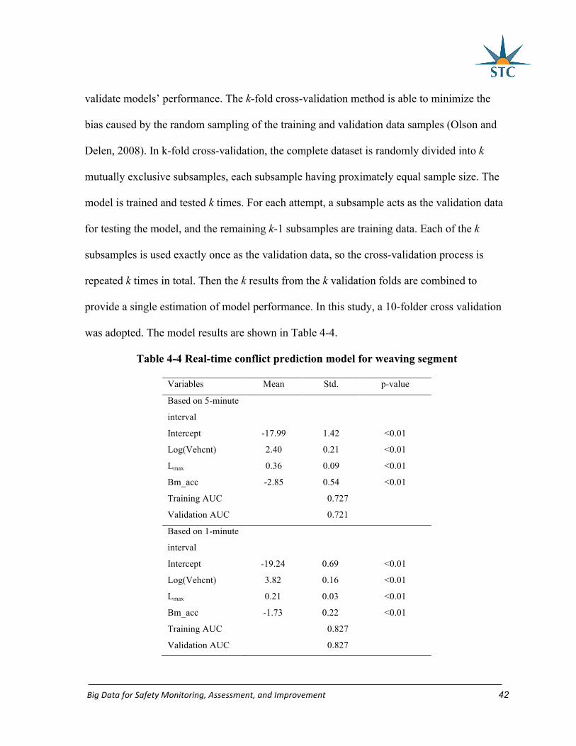
4.4 Model Estimation
In order to find significant conflict precursors and to quantify their impacts on
conflict risk, two logistic regression models were built: one was based on 5-minute intervals;
the other one was based on 1-minute intervals. K-folder cross validation method was used to
BigDataforSafetyMonitoring,Assessment,andImprovement 42
validate models’ performance. The k-fold cross-validation method is able to minimize the
bias caused by the random sampling of the training and validation data samples (Olson and
Delen, 2008). In k-fold cross-validation, the complete dataset is randomly divided into k
mutually exclusive subsamples, each subsample having proximately equal sample size. The
model is trained and tested k times. For each attempt, a subsample acts as the validation data
for testing the model, and the remaining k-1 subsamples are training data. Each of the k
subsamples is used exactly once as the validation data, so the cross-validation process is
repeated k times in total. Then the k results from the k validation folds are combined to
provide a single estimation of model performance. In this study, a 10-folder cross validation
was adopted. The model results are shown in Table 4-4.
Table 4-4 Real-time conflict prediction model for weaving segment
Variables Mean Std. p-value
Based on 5-minute
interval
Intercept -17.99 1.42 <0.01
Log(Vehcnt) 2.40 0.21 <0.01
Lmax 0.36 0.09 <0.01
Bm_acc -2.85 0.54 <0.01
Training AUC 0.727
Validation AUC 0.721
Based on 1-minute
interval
Intercept -19.24 0.69 <0.01
Log(Vehcnt) 3.82 0.16 <0.01
Lmax 0.21 0.03 <0.01
Bm_acc -1.73 0.22 <0.01
Training AUC 0.827
Validation AUC 0.827

BigDataforSafetyMonitoring,Assessment,andImprovement 43
Area Under the Curve (AUC) is a good inex of classification accuracy for logistic
regression models (Hosmer Jr et al., 2013). It plots true positive rate against false positive
rate for all possible thresholds. The range of AUC is 0.5 to 1.0, a higher value indicating a
better ability in discriminating conflict and non-conflict events. When the AUC of a model is
higher than 0.80, it indicates the model has a good discrimination between case and control
(Hosmer Jr et al., 2013).
Both the 5-minute interval and 1-minute interval models showed that the Logarithm
of vehicle count, maximum influence length, and average acceleration at the beginning of
weaving segments were conflict precursors that were significant at the 5% confidence
interval. The 1-minute interval model performed better than the 5-minute interval model by
providing higher training and validation AUCs. Compared to the model using traffic
aggregated at a 5-minute interval, the model using 1-minute interval traffic was able to
capture information that is more detailed.
The coefficients of significant variables in the two models vary. The main reason
might be the way through which traffic was aggregated. From the standard deviations of the
coefficients, it could be found that the 1-minute interval model provided lower standard
deviations than the 5-minute interval model, which indicates that the 1-minute interval model
is more reliable than the 5-minute interval model. It is not hard to understand, the disruptive
traffic 0-1 minutes before a conflict can better present the traffic condition contributing to the
conflict than the disruptive traffic 0-5 minutes before the conflict.
The Logarithm of vehicle count was positively related to conflict risk. When vehicle
count increases, the exposure increases and then the conflict likelihood increases. The
maximum influence length was with a positive sign. A longer influence distance is because
BigDataforSafetyMonitoring,Assessment,andImprovement 44
of a higher percentage of weaving volume. High weaving volume indicates high on-ramp or
off-ramp volume or both. For on-ramp vehicles, they need to accelerate to merge into
mainline traffic; for off-ramp vehicles, they have to diverge from mainline and decelerate to
adjust to low speed limits on off-ramps; meanwhile, high on- and off-ramp traffic volume
also rises weaving opportunity. The acceleration, deceleration, weaving, merging, and
diverging actions definitely worsen traffic safety. Additionally, the average acceleration at
the beginning of weaving segment was proven to have a significantly negative impact on
conflict risk, which means an increase of average acceleration decreases conflict risks.
4.5 Summary
There has been plenty of traffic safety research based on surrogate safety measures.
One of the most commonly used surrogate safety measures is traffic conflicts. The majority
of previous conflict studies focused on conflict frequencies but did not explore conflict
mechanisms from a microscopic aspect. This chapter built a real-time conflict prediction
model for weaving segments based on the traffic and conflict information captured from
microscopic VISSIM network. The simulation network was well calibrated and validated
because of high-resolution big traffic data input.
Driving behavior parameters in simulation were adjusted to validate the simulation
network. When DLCD was 300 meters, CC0 was 1.5 meters, CC1 was 1.5 seconds, and CC2
was 4 meters, not only the traffic condition but also the safety condition of simulated network
were consistent with the field weaving segment network. The validated VISSIM network had
an overall average GEH value of 1.82 and the average speed difference was 2.00 mph. The

BigDataforSafetyMonitoring,Assessment,andImprovement 45
Spearman rank correlation test was carried out to compare the simulated and filed safety, the
coefficient was 0.506 and was significant at the 5% confidence interval.
Two conflict prediction models were estimated, one was based on a 5-minute interval
and the other was based on a 1-minute interval. In both models, Logarithm of vehicle count,
maximum influence length, and average acceleration at the beginning of weaving segment
were significant variables. The model performance of the 1-minute interval model was better
than that of the 5-minute interval model by providing higher AUCs and lower standard
deviation of variable coefficients.
This study is the first one which use the simulated conflict to study the traffic
parameters’ impacts on safety in real-time. Before this study, if researchers intended to build
the real-time safety prediction model, several months’ crash and traffic data for several
locations should be prepared to obtain enough sample size. The traffic data had to be
collected continuously and be with high resolution. If the funding is limited, it is hard to
equip road facilities with enough traffic detectors. Hence, implementing simulation to study
the real-time safety analysis might be an economic, time saving, and reliable method.
BigDataforSafetyMonitoring,Assessment,andImprovement 46
CHAPTER5:TRAVELTIMERELIABILITYANDTRAFFICSAFETY
5.1 Introduction
With a steady growth of traffic demands in urban areas, toll expressways have
become an important alternative for transportation agencies to provide motorists with safe,
efficient, and reliable trips. Three major focus of traffic operators are reducing crash
occurrence, decreasing congestion, and improving travel time reliability on the highway
systems. These three aspects might be interrelated. In other words, an aspect might have an
effect on the others. For instance, crashes could lead to decreased efficiency and unreliable
travel time; reduced efficiency could increase crash likelihood and lower travel time
reliability; unreliable travel time could cause unstable traffic flow thus affecting efficiency
and safety.
During the past few decades, there have been substantial efforts dedicated to
exploring the crash mechanisms and the relationship between traffic efficiency (e.g., level of
service, congestion) and traffic safety. Nevertheless, no research studies have been done to
investigate how travel time reliability could affect traffic safety on urban expressways. The
objective of this chapter is thus to identify whether travel time reliability has impacts on
crash frequency and crash risk for expressways.
5.2 Background
Travel time reliability indicates the level of consistency in transportation service
experienced by travelers compared with their normal experience. Given travel time data,
various approaches have been proposed to measure the travel time reliability. Three types of

BigDataforSafetyMonitoring,Assessment,andImprovement 47
measures could be generalized, namely statistical range measures, buffer measures, and tardy
trip indicators (Martchouk, 2009). One of the statistical range measures is the Percent
Variation as shown in Eq. 5-1 (Lomax and Margiotta, 2003).
!"#$"%&()#*)&*+% = -./01/213456/.6707892/54:96;4<542/=492/54:96;4 ×100% (5-1)
The Buffer Index in Eq. 5-2 is a buffer measure to assess how much extra time is
needed for uncertainty in the travel conditions (Martchouk, 2009).
95 100%th Percentile Travel Time Average Travel TimeBuffer Index
Average Travel Time−
= × (5-2)
Tardy trip indicators imply the amount of late trips. The Misery Index as displayed in
Eq. 5-3 is a tardy trip indicator that compares the worst 20% of the trips against the average
condition to show the impact of late traffic on reliability (Lomax and Margiotta, 2003).
20% 100%Average of the Travel Time for the Longest of Trips Average Travel Time for All TripsMisery Index
Average Travel Time for All Trips−
= × (5-3)
The indicator Percent Variation is easy for calculation and interpretation; meanwhile,
it can be used in real-time analysis. However, it has a drawback since it treats early and late
arrivals equally whereas in reality the public is more concerned about late arrivals. On the
other hand, the Buffer Index and Misery Index focus on the impact of late arrivals on travel
time reliability, but they are hard to be implemented in real-time analysis, since the
calculation of Buffer Index and Misery Index requires large samples to reduce the possibility
that individual observations have significant impacts on calculation results. Hence, the crash
frequency study implemented the three indicators; whereas, the real-time safety analysis only
adopted Percent Variation.
BigDataforSafetyMonitoring,Assessment,andImprovement 48
In some existing studies (Geedipally and Lord, 2010; Yu and Abdel-Aty, 2013a),
there have already been discussions about different mechanisms between SV and MV
crashes. For the purpose of this chapter, whether travel time reliability would have impact on
SV and MV crashes in the same manner is worth investigation. Additionally, real-time crash
analysis was utilized to estimate MV crash risk given a crash occurrence.
5.3 Data Preparation
SR 408, a 22-mile urban expressway, was selected as a study area. The expressway of
interest is traveled by a large number of commuters and experiences heavy congestions
during morning and evening peak hours. Hence, travel time reliability varies across time of
day and across segments of the expressway. Three types of data were collected for SR 408:
traffic, crash, and geometry.
Part of traffic data are from AVI system, which is used as ETC for toll expressways.
For SR 408, most of the travelers (about 85%) have installed AVI tags in their vehicles for
ETC. By collecting the travel time stamps of the encrypted individual vehicles at different
locations, vehicles’ travel time and speed information on a segment are readily available. The
calculations of travel time and speed are as follows,
downstream upstreamTraval Time Timestamp Timestamp= − (5-4)
downstream upstreamMilepost MilepostSpeed
Travel Time
−= (5-5)
The AVI data have been collected since September 2012. At the time of study, data of
two years and seven months until March 2015 were prepared. On the 22-mile expressway,
there were 42 activate AVI segments with 22 on the eastbound and 20 on the westbound in
BigDataforSafetyMonitoring,Assessment,andImprovement 49
the study period. Based on the AVI data, average speed, standard deviation of speed, and the
three indicators, i.e., Percent Variation, Buffer Index, and Misery Index, were calculated.
Since the AVI system only detects vehicles equipped with tags but cannot detect all
vehicles, the traffic volumes on each AVI segment cannot be obtained from AVI but were
derived from the MVDS detectors, which are capable of detecting all vehicles. There were
about 55 MVDS detectors on each direction of SR 408. When there were one or more MVDS
detectors within an AVI segment, the average volume per lane from multiple locations would
be calculated. If there were no MVDS detectors exists within an AVI segment, the average
volume per lane from the nearest upstream and downstream MVDS detectors was used.
Meanwhile, crash data were prepared from S4A database. The crash data provide
crash time, location, passenger numbers, and roadway surface condition (i.e., wet or dry), etc.
For SR 408, 1,342 crashes occurred on the expressway mainline during the study period,
among which 1,112 were MV crashes and 230 crashes were SV crashes. According to the
crash counts, it can be found that the majority of crashes on this urban expressway were MV
crashes, which might imply distinct mechanisms for these two types of crashes.
In addition to traffic data, roadway geometric characteristics are also significant crash
contributing factors (Shankar et al., 1995; Ahmed et al., 2011; Yu et al., 2013). In this task,
geometric data for the expressway were downloaded from FDOT RCI database.
Homogeneous segments of the roadway were generated according to their geometric
characteristics. Short distance segments (less than 0.1 mile) were combined with adjacent
segment, which is with higher similarity. The chosen geometric characteristics included
number of lanes, existence of auxiliary lanes, speed limit, horizontal degree of curvature,
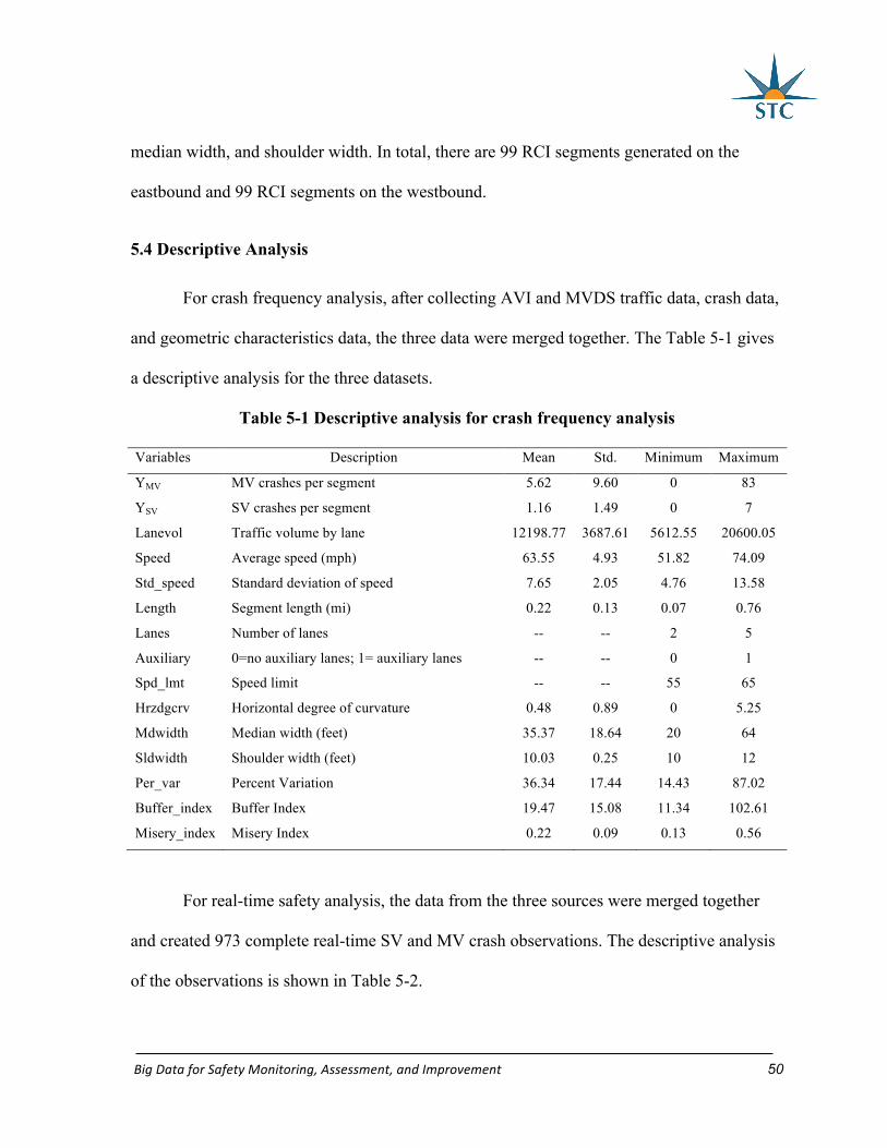
BigDataforSafetyMonitoring,Assessment,andImprovement 50
median width, and shoulder width. In total, there are 99 RCI segments generated on the
eastbound and 99 RCI segments on the westbound.
5.4 Descriptive Analysis
For crash frequency analysis, after collecting AVI and MVDS traffic data, crash data,
and geometric characteristics data, the three data were merged together. The Table 5-1 gives
a descriptive analysis for the three datasets.
Table 5-1 Descriptive analysis for crash frequency analysis
Variables Description Mean Std. Minimum Maximum
YMV MV crashes per segment 5.62 9.60 0 83
YSV SV crashes per segment 1.16 1.49 0 7
Lanevol Traffic volume by lane 12198.77 3687.61 5612.55 20600.05
Speed Average speed (mph) 63.55 4.93 51.82 74.09
Std_speed Standard deviation of speed 7.65 2.05 4.76 13.58
Length Segment length (mi) 0.22 0.13 0.07 0.76
Lanes Number of lanes -- -- 2 5
Auxiliary 0=no auxiliary lanes; 1= auxiliary lanes -- -- 0 1
Spd_lmt Speed limit -- -- 55 65
Hrzdgcrv Horizontal degree of curvature 0.48 0.89 0 5.25
Mdwidth Median width (feet) 35.37 18.64 20 64
Sldwidth Shoulder width (feet) 10.03 0.25 10 12
Per_var Percent Variation 36.34 17.44 14.43 87.02
Buffer_index Buffer Index 19.47 15.08 11.34 102.61
Misery_index Misery Index 0.22 0.09 0.13 0.56
For real-time safety analysis, the data from the three sources were merged together
and created 973 complete real-time SV and MV crash observations. The descriptive analysis
of the observations is shown in Table 5-2.
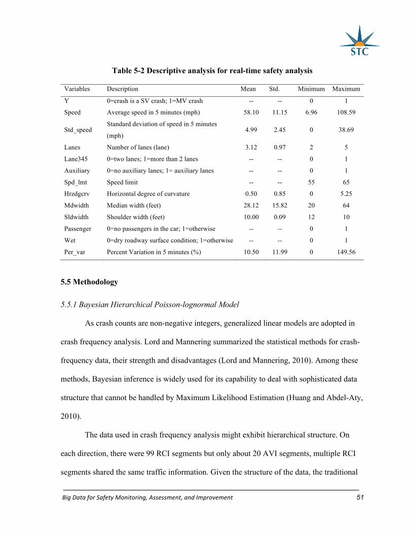
BigDataforSafetyMonitoring,Assessment,andImprovement 51
Table 5-2 Descriptive analysis for real-time safety analysis
Variables Description Mean Std. Minimum Maximum
Y 0=crash is a SV crash; 1=MV crash -- -- 0 1
Speed Average speed in 5 minutes (mph) 58.10 11.15 6.96 108.59
Std_speed Standard deviation of speed in 5 minutes
(mph) 4.99 2.45 0 38.69
Lanes Number of lanes (lane) 3.12 0.97 2 5
Lane345 0=two lanes; 1=more than 2 lanes -- -- 0 1
Auxiliary 0=no auxiliary lanes; 1= auxiliary lanes -- -- 0 1
Spd_lmt Speed limit -- -- 55 65
Hrzdgcrv Horizontal degree of curvature 0.50 0.85 0 5.25
Mdwidth Median width (feet) 28.12 15.82 20 64
Sldwidth Shoulder width (feet) 10.00 0.09 12 10
Passenger 0=no passengers in the car; 1=otherwise -- -- 0 1
Wet 0=dry roadway surface condition; 1=otherwise -- -- 0 1
Per_var Percent Variation in 5 minutes (%) 10.50 11.99 0 149.56
5.5 Methodology
5.5.1 Bayesian Hierarchical Poisson-lognormal Model
As crash counts are non-negative integers, generalized linear models are adopted in
crash frequency analysis. Lord and Mannering summarized the statistical methods for crash-
frequency data, their strength and disadvantages (Lord and Mannering, 2010). Among these
methods, Bayesian inference is widely used for its capability to deal with sophisticated data
structure that cannot be handled by Maximum Likelihood Estimation (Huang and Abdel-Aty,
2010).
The data used in crash frequency analysis might exhibit hierarchical structure. On
each direction, there were 99 RCI segments but only about 20 AVI segments, multiple RCI
segments shared the same traffic information. Given the structure of the data, the traditional

BigDataforSafetyMonitoring,Assessment,andImprovement 52
assumption about the independent sample in regression models does not hold. To properly
evaluate the effects of traffic variables, the hierarchical data structure needs to be addressed.
In this study, a Bayesian hierarchical Poisson-lognormal model framework was
adopted. The introduction of lognormal random effects was to solve the issue of over-
dispersion. The model specification is set up as:
~ ( )ij ijY Poisson λ (5-6)
0 [ ]log( )ij j i ij iXλ α α β ε= + + + (5-7)
j jUα γ= (5-8)
where ijY is the observed crash frequency on RCI segment i (i=1,2,…,198) nested
within AVI segment j (j=1,2,…,42) that follows Poisson distribution with parameter ijλ . 0α
stands for intercept. ijX are geometric characteristics variables and β are the corresponding
coefficients. The random effects follows normal distribution ~ (0,1/ )i iNε τ . jα represents
the effects of AVI traffic variables jU . γ is coefficients for jU . The models were calibrated
with non-informative prior distributions in WinBUGS software (Lunn et al., 2000). β and γ
are assigned with 6(0,10 )N and 3 3~ (10 ,10 )i gammaτ − − .
5.5.2 Logistic Regression Model
Logistic regression models have been widely used in real-time crash studies (Abdel-
Aty and Pande 2005, Hourdos et al. 2006). They are capable to distinguish and quantify crash
contributing parameters. For any given crash event i, it has two exclusive states: MV crash or

BigDataforSafetyMonitoring,Assessment,andImprovement 53
SV crash. In this task, the binary responses, MV crash (yi=1) and SV crash (yi=0), were
converted into probabilities pi (yi=1) and 1-pi (yi=0), respectively. The model is as follows,
~ ( )i iy Bernoulli p (5-9)
01
log( )1
Ri
r riri
px
pβ β
=
= +− ∑ (5-10)
where 0β is the intercept, rβ the coefficient of rth predictors, rix the value of rth
explanatory variable for ith observation. The logistic regression model was calibrated in SAS
software using PROC LOGISTIC.
5.6 Model Results
5.6.1 Crash Frequency Analysis
In Bayesian inference, Deviance Information Criterion (DIC) was adopted for model
performance evaluation. DIC is the summation of model fitting and the number of effective
variables. Smaller DIC is better. Percent Variation, Buffer Index, and Misery Index were
individually included in the crash frequency models for MV and SV crashes in Table 5-3 and
Table 5-4.
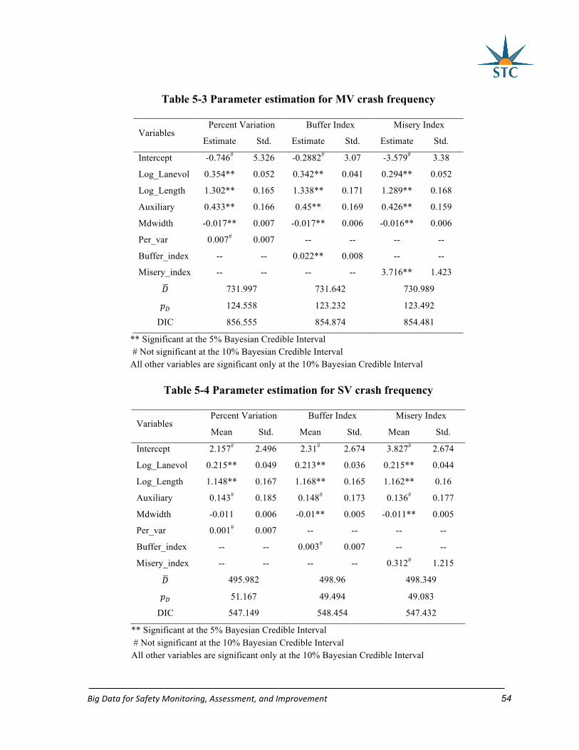
BigDataforSafetyMonitoring,Assessment,andImprovement 54
Table 5-3 Parameter estimation for MV crash frequency
Variables Percent Variation Buffer Index Misery Index
Estimate Std. Estimate Std. Estimate Std.
Intercept -0.746# 5.326 -0.2882# 3.07 -3.579# 3.38
Log_Lanevol 0.354** 0.052 0.342** 0.041 0.294** 0.052
Log_Length 1.302** 0.165 1.338** 0.171 1.289** 0.168
Auxiliary 0.433** 0.166 0.45** 0.169 0.426** 0.159
Mdwidth -0.017** 0.007 -0.017** 0.006 -0.016** 0.006
Per_var 0.007# 0.007 -- -- -- --
Buffer_index -- -- 0.022** 0.008 -- --
Misery_index -- -- -- -- 3.716** 1.423
B 731.997 731.642 730.989
C3 124.558 123.232 123.492
DIC 856.555 854.874 854.481
** Significant at the 5% Bayesian Credible Interval # Not significant at the 10% Bayesian Credible Interval All other variables are significant only at the 10% Bayesian Credible Interval
Table 5-4 Parameter estimation for SV crash frequency
Variables Percent Variation Buffer Index Misery Index
Mean Std. Mean Std. Mean Std.
Intercept 2.157# 2.496 2.31# 2.674 3.827# 2.674
Log_Lanevol 0.215** 0.049 0.213** 0.036 0.215** 0.044
Log_Length 1.148** 0.167 1.168** 0.165 1.162** 0.16
Auxiliary 0.143# 0.185 0.148# 0.173 0.136# 0.177
Mdwidth -0.011 0.006 -0.01** 0.005 -0.011** 0.005
Per_var 0.001# 0.007 -- -- -- --
Buffer_index -- -- 0.003# 0.007 -- --
Misery_index -- -- -- -- 0.312# 1.215
B 495.982 498.96 498.349
C3 51.167 49.494 49.083
DIC 547.149 548.454 547.432
** Significant at the 5% Bayesian Credible Interval # Not significant at the 10% Bayesian Credible Interval All other variables are significant only at the 10% Bayesian Credible Interval

BigDataforSafetyMonitoring,Assessment,andImprovement 55
In the MV crash frequency model, logarithmic volume per lane positively affects the
crash frequency. Meanwhile, the logarithmic segment length, median width, and existence of
auxiliary lanes are significant geometric characteristics. Traffic volume and segment length
are the most common exposure variables in previous traffic safety analysis, of which many
suggested that crash count is not linearly proportional to volume and segment length thus the
logarithmic transformation was applied (Ahmed et al., 2011). The effects of median width
and existence of auxiliary lanes are consistent with existing studies (Shi and Abdel-Aty,
2015). The median width has negative effect on crash frequency since it provides more space
for vehicle leeway to avoid a crash. The auxiliary lanes provide turning movements near
expressway ramps where speed changes and lane changes are required. The speed change
actions might result in rear-end crashes, and lane change maneuvers might cause sideswipe
crashes.
The modeling results of MV crash frequency study also confirmed that travel time
reliability has an impact on MV crash count. Comparing the performances of Percent
Variation, Buffer Index, and Misery Index in the models, both Buffer Index and Misery
Index were found to be significant at the 5% Bayesian Credible Interval while Percent
Variation was not. The different performances of indicators in the models might originate
from their definitions. Both Buffer Index and Misery Index emphasize the effects of late
arrivals on travel time reliability. In contrast, Percent Variation treats early and late arrivals
equally. For most motorists, the risk and cost of early and late arrivals could be distinct. Late
arrivals are more likely to cause anxiety and risky behaviors than early arrivals. In summary,
as reflected in the significance of the three variables, lower travel time reliability caused by
delayed trips would pose more challenges to traffic safety. Consequently, to better capture
BigDataforSafetyMonitoring,Assessment,andImprovement 56
how travel time reliability affects crash frequency, the use of Buffer Index and Misery Index
are recommended.
The parameter estimation for SV crashes is different from that for MV crashes. As
exposure variables, higher values of logarithmic segment length and traffic volume per lane
are related with more SV crashes. The effects of median width remain the same for both SV
and MV crashes. The differences between these two types of crashes are mainly reflected by
auxiliary lanes and travel time reliability. For SV crashes, existence of auxiliary lanes is no
longer significant. Such result is expected as merging and diverging on the segments with
auxiliary lanes would be more likely to cause MV crashes rather than SV crashes. Travel
time reliability, unlike their effects on MV crashes, does not have significant impact on SV
crashes. SV crashes are more likely to occur under free flow conditions, under which travel
time might be more stable. Given the estimation results of SV and MV crashes, it is obvious
that travel time reliability has greater effects on MV crashes than SV crashes.
5.6.2 Real-Time Crash Analysis
For the logistic regression model, in order to prevent high correlation between
variables, the Pearson Correlation test was done before the modelling process. If the absolute
of the correlation coefficient value of two continuous parameters was higher than 0.3, or
when the chi-square test showed two categorical variables were significantly related, only the
variable which resulted in a higher AUC was kept in the model. The range of AUC is 0.5 to
1.0, a higher value indicating a better ability in discriminating MV and SV crashes in this
study. The model estimation is in Table 5-5.
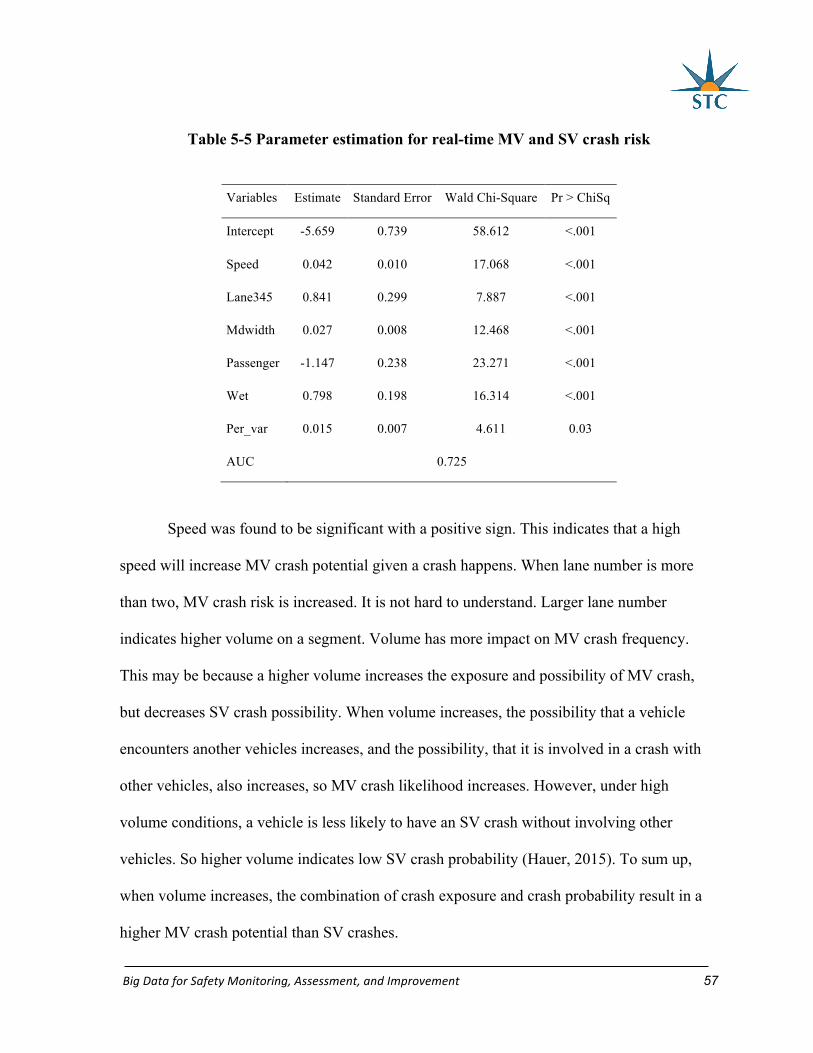
BigDataforSafetyMonitoring,Assessment,andImprovement 57
Table 5-5 Parameter estimation for real-time MV and SV crash risk
Variables Estimate Standard Error Wald Chi-Square Pr > ChiSq
Intercept -5.659 0.739 58.612 <.001
Speed 0.042 0.010 17.068 <.001
Lane345 0.841 0.299 7.887 <.001
Mdwidth 0.027 0.008 12.468 <.001
Passenger -1.147 0.238 23.271 <.001
Wet 0.798 0.198 16.314 <.001
Per_var 0.015 0.007 4.611 0.03
AUC 0.725
Speed was found to be significant with a positive sign. This indicates that a high
speed will increase MV crash potential given a crash happens. When lane number is more
than two, MV crash risk is increased. It is not hard to understand. Larger lane number
indicates higher volume on a segment. Volume has more impact on MV crash frequency.
This may be because a higher volume increases the exposure and possibility of MV crash,
but decreases SV crash possibility. When volume increases, the possibility that a vehicle
encounters another vehicles increases, and the possibility, that it is involved in a crash with
other vehicles, also increases, so MV crash likelihood increases. However, under high
volume conditions, a vehicle is less likely to have an SV crash without involving other
vehicles. So higher volume indicates low SV crash probability (Hauer, 2015). To sum up,
when volume increases, the combination of crash exposure and crash probability result in a
higher MV crash potential than SV crashes.
BigDataforSafetyMonitoring,Assessment,andImprovement 58
Additionally, the median width has a positive sign, indicates that a segment with a
narrow median width increase the SV crash risk. One of main reason for the occurrence of
SV crashes is vehicle out of control. A wider median width could decrease SV crash risk by
providing drivers with more leeway to regained control of vehicles. On the other hand,
median width might not have as much impact on MV crashes as on SV crashes, because MV
crashes are mainly because of danger interactions between vehicles, such as too close car
following.
Furthermore, it was revealed that the presence of passenger was found to increase SV
crash risk by having a significant negative coefficient. Drivers might be distracted by
passenger(s) and out of control vehicle. Wet roadway surface condition might increase MV
crash risks. Wet roadway surface has smaller friction and may result in longer braking
distance than on dry surface. However, under wet roadway surface condition, drivers might
keep the same following distances as under dry condition, and vehicles run into a heading
vehicle because of long braking distance. Hence, wet roadway surface condition significantly
increases MV crash risk.
The Percent Variation was statistically positive related to MV crash risk. A higher
Percent Variation indicates that behaviors of motorists could vary substantially. On the other
hand, SV crashes are more likely to occur under free flow conditions, under which condition
travel time might be more stable. This result further confirms the conclusion from the crash
frequency prediction models: travel time reliability has different impact on MV and SV
crashes.

BigDataforSafetyMonitoring,Assessment,andImprovement 59
5.7 Summary
The reduced travel time reliability could cause unstable traffic flow thus affects
efficiency and safety. In this task, MV and SV crash data on SR 408 have been collected. The
different MV and SV crash frequencies indicated that the crashes mechanisms for MV and
SV crashes might not be the same. Hence, the project has worked on crash frequency and
real-time crash analysis for MV and SV crash using travel time reliability indicators: Percent
Variation, Buffer Index, and Misery Index. The three indicators were used in crash frequency
study, but only Percent Variation was used in real-time safety analysis because the other two
indicators are not suitable to be used in real-time analysis.
Two Bayesian Hierarchical Poisson-lognormal models were developed to predict SV
and MV crash frequencies separately. The results showed that Buffer Index and Misery Index
had significant positive impact on MV crash frequency; however, Percent Variation was not
significant. On the other hand, all the indicators were not significantly related to SV crash
frequency. Then, a logistic regression model was built to evaluate the quantitative impact of
Percent Variation on MV crash risk give a crash occurrence. The results showed that high
Percent Variation, indicating low travel time reliability, would increase MV crash risk.
At present, many toll expressway agencies provide travelers with estimated real-time
travel time and congestion warning using dynamic message signs. This is beneficial to help
road users prepare for current traffic conditions and adjust their driving accordingly. Thus,
the study has found that improving travel time reliability would decrease MV crash potential.
Given the high proportion of MV crashes on expressways, it is expected that reduction of
MV crashes will remarkably improve safety.

BigDataforSafetyMonitoring,Assessment,andImprovement 60
CHAPTER6:REAL-TIMEEVALUATIONFORRAMPCRASHES
6.1 Introduction
There have been numerous studies on real-time crash prediction models with the
intention to link real-time crash likelihood with various predictors. The underlying
assumption of these studies is that some predictors, called crash precursors, are relatively
more ‘crash prone’ than other parameters. Among the studied traffic predictors, the standard
deviation of speed, traffic volume, and traffic density were common significant crash
precursors (Lee et al., 2002; Abdel-Aty and Pande, 2005). Additonally, geometric parameters
play important roles in the occurrence of crashes (Wang et al., 2015a).
However, the human factors’ impact has not been widely examined in real-time
safety studies. There are two types of events in real-time safety analyses: crash and non-crash
events. For crash events, crash reports can provide information for drivers who are involved
in a traffic crash. On the other hand, for non-crash events, driver information cannot be
obtained from available data sources. Hence, real-time crash risk analysis is unable to
consider driver characteristics as explanatory variables. Trip generation and land-use factors
can reflect driver behavior and further reflect their effect on traffic safety. From a
macroscopic perspective of view, trip generation and land-use have already been proven
significant crash frequency contributing factors (Abdel-Aty et al., 2013; Lee et al., 2015a;
Lee et al., 2015b). However, there has been no study, which adopted trip generation and
land-use factors in microscopic traffic safety analyses.
For crashes that happen on ramps, the origins or destinations of the vehicles involved
in the crash are likely to be ramp nearby zones. Hence, if the trip generation and land-use
BigDataforSafetyMonitoring,Assessment,andImprovement 61
information of the zone in which a ramp lies can be captured, these points of data might act
as surrogates of driver characteristics for ramps.
The logistic regression model has been widely used in the analysis of data whose
target variable is binary (Washington et al., 2010). It measures the relationship between the
target variable and explanatory variables based on a logistic function. The model is easy for
interpretation since the model results provide the coefficient value for each significant
variable. However, the logistic regression assumes that the error term has a standard logistic
distribution. In reality, this assumption may not be true. On the other hand, the data mining
method might not be able to provide the impact of each independent variable on the target
variable, but it does not have a restriction on the distribution of parameters. Among
numerous data mining methods, Support Vector Machine (SVM) models have been applied
in several transportation studies, because they can provide high accuracy (Qu et al., 2012).
Hence, this chapter integrated data mining and traditional statistical model (logistic
regression model) to conduct real-time crash analysis for ramps.
6.2 Methodology
6.2.1 Logistic Regression Model
For any given event i, it has two exclusive states: crash or non-crash. In this task, the
binary responses, crash ( iy =1) and non-crash ( iy =0), are converted into probabilities ip ( iy
=1) and 1- ip ( iy =0), respectively. The model is as follows,
~ ( )i iy Bernoulli p (6-11)
01
log( )1
Ri
r riri
px
pβ β
=
= +− ∑ (6-12)

BigDataforSafetyMonitoring,Assessment,andImprovement 62
where 0β is the intercept, rβ the coefficient of rth predictors, rix the value of rth
explanatory variable for ith observation.
6.2.2 Support Vector Machine
SVM is used for classification analysis by constructing a hyperplane or set of
hyperplanes in a high- or infinite-dimensional space (Suykens and Vandewalle, 1999). The
hyperplane with the largest distance to the nearest training-data point is chosen, indicating
that it provides the largest separation between two types of events. There are two sorts of
SVM: linear and nonlinear. The choice of SVM sort is based on the data type, e.g., a linear
SVM is better if data is linearly separated. A nonlinear SVM is achieved by applying a
kernel. By introducing a kernel, SVM is flexible in the choice of the separation form and can
handle nonlinear data (Deng et al., 2012). In this task, a nonlinear SVM is applied.
The crash occurrence outcome y is either 1 (crash) or -1 (non-crash). Training data D
is a set of n points of the form,
( ) { }{ }1
, | , 1,1nP
i i i i iD x y x R y
== ∈ ∈ − (6-13)
where x is the matrix of independent variables and P is the number of significant
variables. The decision function is as follows,
( ) ( )Tf x sign w x b= + (6-14)
1 2[ ... ]Tpω ω ω ω= (6-15)
A hyperplane can be written as the set of points x satisfying
0Tw x b+ = (6-16)

BigDataforSafetyMonitoring,Assessment,andImprovement 63
( )Tiw x b+ should be positive when iy =1, and it should be negative when iy =-1. To
summarize, ( ) 0Ti iy w x b+ > . The decision function is using a sign-function. This results in
an uncertainty of distance or margin (Campbell and Ying, 2011). Hence, two parallel
hyperplanes is constructed (Campbell and Ying, 2011):
1Tw x b+ = (6-17)
and
1Tw x b+ = − (6-18)
The distance between these two hyperplanes is 2w
. The target of SVM is to maximize
the distance between the two hyperplanes by minimizing 212w . In order to prevent data
points from falling into the margin between two hyperplanes, the following constraint is
added:
for each observation i either
1, 1Ti iw x b if y+ ≥ = (6-19)
or
1, 1Ti iw x b if y+ ≤ − = − (6-20)
Combing Eq. 6-9 and 6-10, produce the following new constrain:
( ) 1,Ti iy w x b for all i+ ≥ (6-21)
This is a constrained optimization problem in which 212w is minimized subject to
constrain Eq. 6-11. The optimization problem can be reduced to the minimization of the
following Lagrange function,

BigDataforSafetyMonitoring,Assessment,andImprovement 64
1
1( , ) ( . ) [ ( . ) 1]2
n
i i ii
L w b ww y w x bα=
= − + −∑ (6-22)
where iα are Lagrange multipliers, and iα >0. The Eq. 6-12 is taken the derivatives
with respect to b and w , and set these derivatives to zero:
1
( , ) 0n
i ii
L w b yb
α=
∂= =
∂ ∑ (6-23)
1
( , ) 0n
i i ii
L w bw y x
wα
=
∂= − =
∂ ∑ (6-24)
Substituting Eq. 6-13 and 6-14 back into Eq. 6-12, the formulation is obtained,
1 1 1 1
1 1 1 1 1 1
1 1 1
1( ) ( . ) [ ( . ) 1]21 ( . ) ( . )2
1 ( . )2
n n n n
i j i j i j i i j j j ii j i j
n n n n n n
i j i j i j i j i j i j i i ii j i j i i
n n n
i i j i j i ji i j
W y y x x y y x x b
y y x x y y x x y b
y y K x x
α α α α α
α α α α α α
α α α
= = = =
= = = = = =
= = =
= − + −
= − − +
= −
∑∑ ∑ ∑
∑∑ ∑∑ ∑ ∑
∑ ∑∑
(6-25)
Subject to
10 0
n
i i ii
and yα α=
≥ =∑ (6-26)
Eq. 6-15 shows the linear kernel ( . ) ( . )i j i jK x x x x= , but when the points are not
linearly classified, there is a need to conduct another kernel. In this task, the Gaussian radial
basis kernel was used,
2( . ) exp( ), 0i j i jK x x x x forγ γ= − − > (6-27)
whereγ was set as 0.5. Compared to a linear kernel, the Gaussian radial basis kernel
has been proven better in a real-time safety study by Yu and Abdel-Aty (2013b).
BigDataforSafetyMonitoring,Assessment,andImprovement 65
6.3 Data Preparation
This chapter chose 141 ramps from three expressways in Central Florida: SR 408, SR
417, and SR 528. The study period was from July 2013 to March 2014. Five dataset were
collected: crash, traffic, geometry, trip generation, and land-use data.
The crash data were from S4A. For each crash observation, crash report provided
crash time, coordinate, type and severity, etc. The traffic data were supplied by MVDS
detectors from CFX. The MVDS detectors record aggregated vehicle counts, time mean
speed, and lane occupancy every minute for each lane.
In addition to crash and traffic data, ramp geometric characteristics data were
collected. The shoulder width information was obtained from the FDOT RCI database; ramp
type (on- and off-ramp), ramp configuration (diamond and non-diamond ramp), and presence
of a tollbooth were gathered manually using ArcGIS. The studied ramps exist in 69
SWTAZs. Both trip generation and land-use data of these SWTAZs were from the Florida
Statewide Model from the FDOT Central Office. The trip generation data were estimated
using observed socio-demographic data.
There were 122 crashes documented and matched with traffic, geometry, land-use
and trip generation information. The traffic conditions, which were present 5-10 minutes
before the reported crash time, were used as crash events. For example, if a crash occurs at
8:00 A.M., traffic data extracted are from 7:50 to 7:55 A.M. of the same day. The non-crash
dataset was made up of normal traffic conditions which did not result in a crash or were not
impacted by a crash. In this task, non-crash events were the traffic conditions that were more

BigDataforSafetyMonitoring,Assessment,andImprovement 66
than 2 hours before or after a crash observation at the same ramp. Both crash and non-crash
events were aggregated into 5-minute intervals to mitigate data noise.
The non-crash dataset consisted of more than 10 million observations. It was not
practical to use the entire non-crash dataset. Hence, this task adopted an unmatched case-
control design. A total of 1,220 controls (non-crash events) were randomly sampled from the
non-crash dataset. Thus, the total number of observations was 122 crash and 1,220 non-crash
events. The descriptive analysis of variables of the final dataset is shown in Table 6-1.
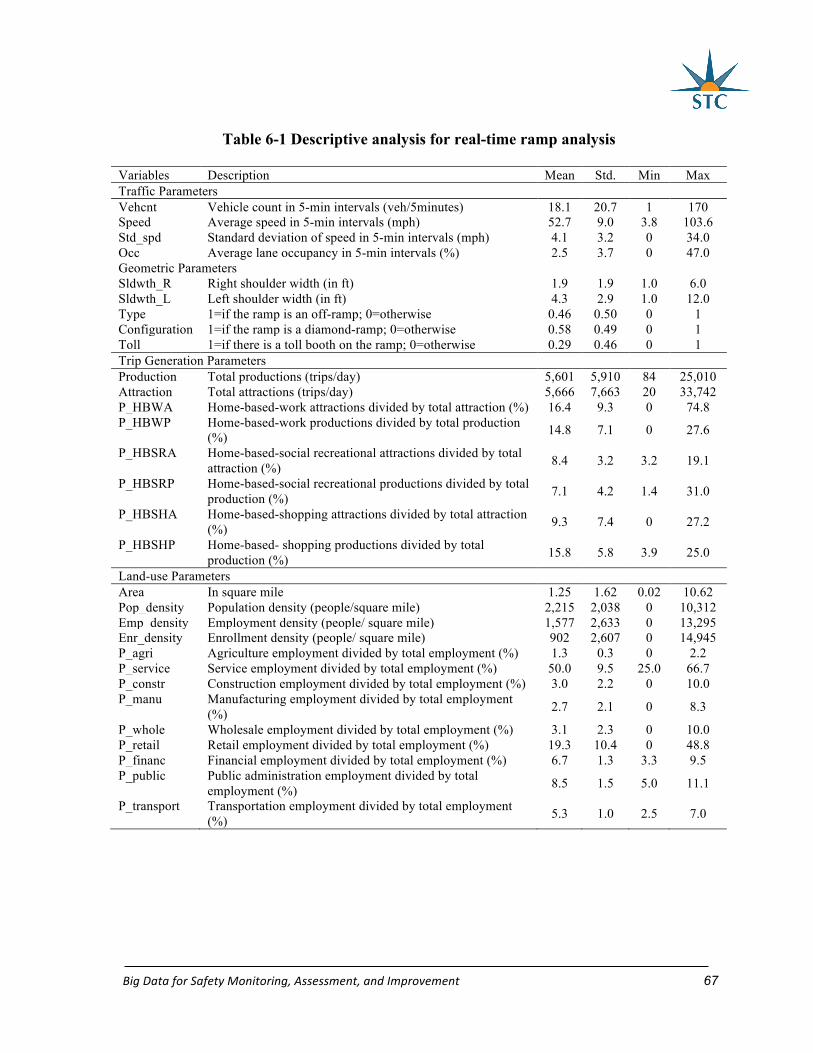
BigDataforSafetyMonitoring,Assessment,andImprovement 67
Table 6-1 Descriptive analysis for real-time ramp analysis
Variables Description Mean Std. Min Max Traffic Parameters Vehcnt Vehicle count in 5-min intervals (veh/5minutes) 18.1 20.7 1 170 Speed Average speed in 5-min intervals (mph) 52.7 9.0 3.8 103.6 Std_spd Standard deviation of speed in 5-min intervals (mph) 4.1 3.2 0 34.0 Occ Average lane occupancy in 5-min intervals (%) 2.5 3.7 0 47.0 Geometric Parameters Sldwth_R Right shoulder width (in ft) 1.9 1.9 1.0 6.0 Sldwth_L Left shoulder width (in ft) 4.3 2.9 1.0 12.0 Type 1=if the ramp is an off-ramp; 0=otherwise 0.46 0.50 0 1 Configuration 1=if the ramp is a diamond-ramp; 0=otherwise 0.58 0.49 0 1 Toll 1=if there is a toll booth on the ramp; 0=otherwise 0.29 0.46 0 1 Trip Generation Parameters Production Total productions (trips/day) 5,601 5,910 84 25,010 Attraction Total attractions (trips/day) 5,666 7,663 20 33,742 P_HBWA Home-based-work attractions divided by total attraction (%) 16.4 9.3 0 74.8 P_HBWP Home-based-work productions divided by total production
(%) 14.8 7.1 0 27.6
P_HBSRA Home-based-social recreational attractions divided by total attraction (%) 8.4 3.2 3.2 19.1
P_HBSRP Home-based-social recreational productions divided by total production (%) 7.1 4.2 1.4 31.0
P_HBSHA Home-based-shopping attractions divided by total attraction (%) 9.3 7.4 0 27.2
P_HBSHP Home-based- shopping productions divided by total production (%) 15.8 5.8 3.9 25.0
Land-use Parameters Area In square mile 1.25 1.62 0.02 10.62 Pop_density Population density (people/square mile) 2,215 2,038 0 10,312 Emp_density Employment density (people/ square mile) 1,577 2,633 0 13,295 Enr_density Enrollment density (people/ square mile) 902 2,607 0 14,945 P_agri Agriculture employment divided by total employment (%) 1.3 0.3 0 2.2 P_service Service employment divided by total employment (%) 50.0 9.5 25.0 66.7 P_constr Construction employment divided by total employment (%) 3.0 2.2 0 10.0 P_manu Manufacturing employment divided by total employment
(%) 2.7 2.1 0 8.3
P_whole Wholesale employment divided by total employment (%) 3.1 2.3 0 10.0 P_retail Retail employment divided by total employment (%) 19.3 10.4 0 48.8 P_financ Financial employment divided by total employment (%) 6.7 1.3 3.3 9.5 P_public Public administration employment divided by total
employment (%) 8.5 1.5 5.0 11.1
P_transport Transportation employment divided by total employment (%) 5.3 1.0 2.5 7.0
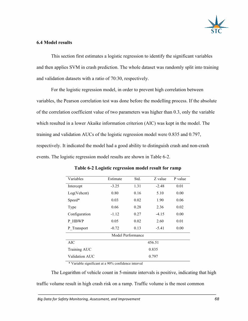
BigDataforSafetyMonitoring,Assessment,andImprovement 68
6.4 Model results
This section first estimates a logistic regression to identify the significant variables
and then applies SVM in crash prediction. The whole dataset was randomly split into training
and validation datasets with a ratio of 70:30, respectively.
For the logistic regression model, in order to prevent high correlation between
variables, the Pearson correlation test was done before the modelling process. If the absolute
of the correlation coefficient value of two parameters was higher than 0.3, only the variable
which resulted in a lower Akaike information criterion (AIC) was kept in the model. The
training and validation AUCs of the logistic regression model were 0.835 and 0.797,
respectively. It indicated the model had a good ability to distinguish crash and non-crash
events. The logistic regression model results are shown in Table 6-2.
Table 6-2 Logistic regression model result for ramp
Variables Estimate Std. Z value P value
Intercept -3.25 1.31 -2.48 0.01
Log(Vehcnt) 0.80 0.16 5.10 0.00
Speed* 0.03 0.02 1.90 0.06
Type 0.66 0.28 2.36 0.02
Configuration -1.12 0.27 -4.15 0.00
P_HBWP 0.05 0.02 2.60 0.01
P_Transport -0.72 0.13 -5.41 0.00
Model Performance
AIC 456.51
Training AUC 0.835
Validation AUC 0.797
* Variable significant at a 90% confidence interval
The Logarithm of vehicle count in 5-minute intervals is positive, indicating that high
traffic volume result in high crash risk on a ramp. Traffic volume is the most common

BigDataforSafetyMonitoring,Assessment,andImprovement 69
exposure variables in previous traffic safety analysis, a significant positive relationship
between traffic volume and crash count or crash risj has been widely found by researchers
(Abdel-Aty and Pande, 2005). Speed was also found to be significant at the 10% confidence
interval with a positive sign. Higher speed definitely increases both braking and reaction
distance. Hence, a vehicle travelling at a higher speed would more likely have a collision
with other objects.
Two geometric factors were found to be significant in the model. The results indicate
that the crash ratio on off-ramps is about 1.93 times higher that of on-ramps. The reason is
that vehicles on the off-ramps need to decelerate to adjust to lower speed limits on ramps;
meanwhile, they have to decrease speed in order to prepare to brake or even stop at the cross-
street intersection. If a following vehicle does not react or decelerate in time, it will collide
with the vehicle ahead. Ramp configuration is significant and proven to be negatively related
to crash likelihood. The odds of a crash on a diamond ramp are 0.33 times of that on non-
diamond ramp. Non-diamond ramps have smaller turning radii, and can lead to a loss of
vehicle control and result in crashes.
The percentage of Home-based-work production is positively related to crash risk.
The Home-based-work production includes two trips, one is from home to work, and the
other is from work to home. First, drivers who travel from home to work have to arrive at
destinations on time. They may want to avoid being late and may rush to get to work. Thus,
they might drive at a higher speed than usual. Second, drivers may be tired after whole day of
work, so the crash potential of work-to-home trip may be higher than other trips.
The most significant land-use parameter is the percentage of transportation
employment. It is interpreted that a higher percentage of transportation employees will
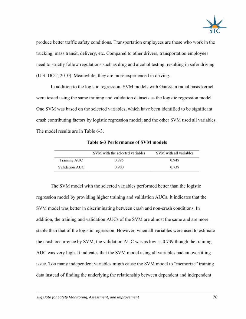
BigDataforSafetyMonitoring,Assessment,andImprovement 70
produce better traffic safety conditions. Transportation employees are those who work in the
trucking, mass transit, delivery, etc. Compared to other drivers, transportation employees
need to strictly follow regulations such as drug and alcohol testing, resulting in safer driving
(U.S. DOT, 2010). Meanwhile, they are more experienced in driving.
In addition to the logistic regression, SVM models with Gaussian radial basis kernel
were tested using the same training and validation datasets as the logistic regression model.
One SVM was based on the selected variables, which have been identified to be significant
crash contributing factors by logistic regression model; and the other SVM used all variables.
The model results are in Table 6-3.
Table 6-3 Performance of SVM models
SVM with the selected variables SVM with all variables
Training AUC 0.895 0.949
Validation AUC 0.900 0.739
The SVM model with the selected variables performed better than the logistic
regression model by providing higher training and validation AUCs. It indicates that the
SVM model was better in discriminating between crash and non-crash conditions. In
addition, the training and validation AUCs of the SVM are almost the same and are more
stable than that of the logistic regression. However, when all variables were used to estimate
the crash occurrence by SVM, the validation AUC was as low as 0.739 though the training
AUC was very high. It indicates that the SVM model using all variables had an overfitting
issue. Too many independent variables migth cause the SVM model to “memorize” training
data instead of finding the underlying the relationship between dependent and independent
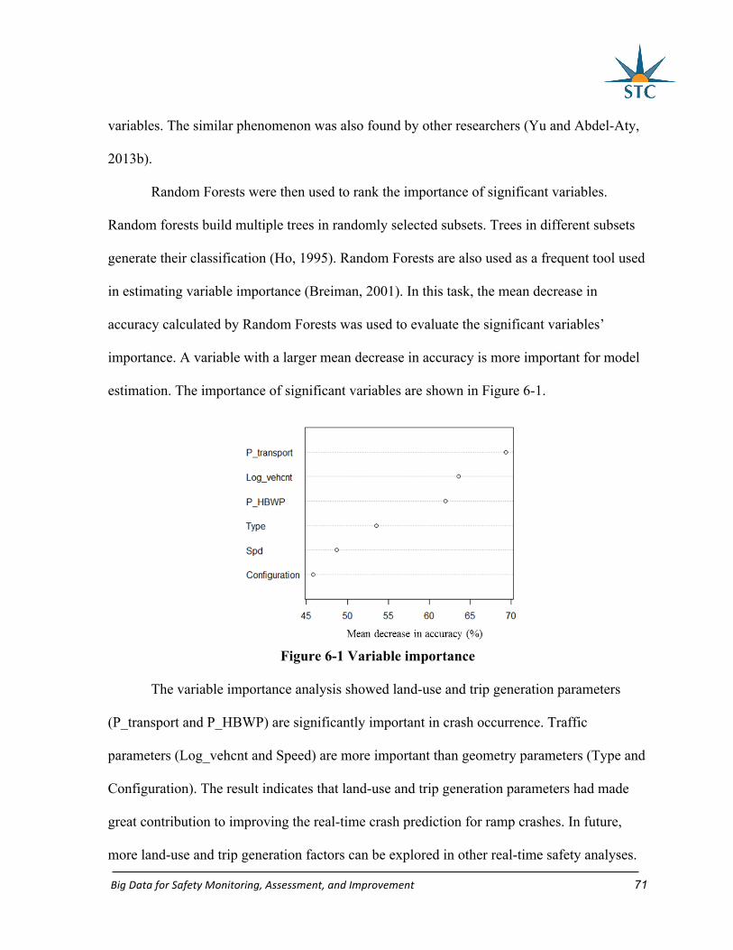
BigDataforSafetyMonitoring,Assessment,andImprovement 71
variables. The similar phenomenon was also found by other researchers (Yu and Abdel-Aty,
2013b).
Random Forests were then used to rank the importance of significant variables.
Random forests build multiple trees in randomly selected subsets. Trees in different subsets
generate their classification (Ho, 1995). Random Forests are also used as a frequent tool used
in estimating variable importance (Breiman, 2001). In this task, the mean decrease in
accuracy calculated by Random Forests was used to evaluate the significant variables’
importance. A variable with a larger mean decrease in accuracy is more important for model
estimation. The importance of significant variables are shown in Figure 6-1.
Figure 6-1 Variable importance
The variable importance analysis showed land-use and trip generation parameters
(P_transport and P_HBWP) are significantly important in crash occurrence. Traffic
parameters (Log_vehcnt and Speed) are more important than geometry parameters (Type and
Configuration). The result indicates that land-use and trip generation parameters had made
great contribution to improving the real-time crash prediction for ramp crashes. In future,
more land-use and trip generation factors can be explored in other real-time safety analyses.
BigDataforSafetyMonitoring,Assessment,andImprovement 72
6.5 Summary
Previous studies found that several real-time traffic and environmental factors are
significant crash precursors. However, no study has been conducted to analyze the impact of
land-use and trip generation parameters on crash risk. This chapter explored real-time crash
risk for expressway ramps using traffic, geometric, land-use, and trip generation predictors.
A logistic regression model was utilized to find the significant variables. The model
identified that volume and speed have a positive impact on crash risk. It also indicated that
off-ramps and non-diamond ramps also significantly increase the crash risk. As for the trip
generation parameters, the percentage of home-based-work production compared to other
trip-generation parameters was found to have a positive impact on crash risk. The percentage
of transportation employment was negatively related to crash risk.
Subsequently, two SVM models were applied to predict crash occurrence: one with
all variables and the other only with significant variables identified by the logistic regression
model. It was found that the SVM model with identified significant variables outperformed
the logistic regression model by providing higher and more stable AUCs. However, the SVM
model with all variables might have an overfitting issue as it provided high training AUC but
lower validation AUC. Therefore, instead of using all collected variables, it would be better
to build SVM models based on significant variables identified by other models such as the
logistic regression models. Meanwhile, Random Forests were used to rank the significant
variables’ importance, the result showed that land-use and trip generation parameters were
parameters with high importance.
BigDataforSafetyMonitoring,Assessment,andImprovement 73
CHAPTER7:INTERSECTIONSAFETYPERFORMANCEFUNCTIONS
7.1 Introduction
A series of safety performance functions (SPFs) have been developed for different
facilities for various crash types. Highway Safety Manual (HSM) (AASHTO, 2010)provides
a range of segment- and intersection-based SPFs for many facility types including but not
limited to rural two-lane two-way roads, rural multilane highways, and urban and suburban
arterials. According to the HSM (AASHTO, 2010), the SPFs play a key role in identifying
crash hotspots (i.e., screening), and evaluating safety countermeasures using the empirical
Bayes method. A majority of the SPFs have been built at the micro-level, such as
intersection, segment, or corridor level. On the other hand, some researchers have estimated
SPFs at the macro-level (e.g., traffic analysis zones) to incorporate highway safety in the
long-term transportation planning process.
A need of incorporating roadway safety considerations in long-term transportation
planning process has been emphasized in the last decades in accordance with Moving Ahead
for Progress in the 21st Century Act (MAP-21 Act) and Fixing America’s Surface
Transportation Act (FAST Act). This integration planning process is called transportation
safety planning or macroscopic traffic safety analysis. Incorporating safety in the long-term
transportation plans has been a vital issue. Safety is being used as one of the performance
measures in transportation improvement program and in more advanced planning efforts,
such as scenario planning at the Metropolitan Planning Organization (MPO) level. Therefore,
transportation engineers need to place more efforts to improve traffic safety problems along

BigDataforSafetyMonitoring,Assessment,andImprovement 74
with the long-term transportation planning and this is the main reason that the macroscopic
safety studies have emerged since the last decade.
Although numerous macro-level studies have found that a variety of demographic and
socioeconomic zonal characteristics have substantial effects on traffic safety, few studies
have attempted to coalesce micro-level with macro-level data for estimating SPFs. Abdel-Aty
et al. (2016) and Lee (2014)proposed a methodology to integrate macro-level and micro-
level data to provide a comprehensive perspective by balancing the two-levels. Still, their
methodology is based on the macro-level SPFs. Park et al. (2015) estimated segment-level
SPFs to evaluate the effectiveness of bicycle facilities. The authors included block-group
based macro-level data including population density and income and found that the macro-
level parameters were statistically significant in the segment-level SPFs. Recently, Huang et
al. (2016) estimated SPFs separately at micro-level and macro-level and compared the model
performance. The results indicated that the micro-level model had a better fit and
performance. The authors claimed that the micro-level approach was able to provide better
insights on microscopic factors that directly contributed to traffic crashes; while, the macro-
level approach was beneficial when monitoring regional safety and relating it with socio-
demographic factors.
Huang and Abdel-Aty (2010) discussed the multi-level data in traffic safety. The
multi-level included occupant, driver/vehicle, crash, site, geographic region, and the extra
temporal dimension. The authors suggested many ideas to explore crashes at the multi-level.
For instance, analyzing traffic crash counts 1) at intersection and time-level; 2) at county and
corridor-level; 3) at county level with spatial effect; and so on. Guo et al. (2010) developed
several SPFs for signalized intersections with corridor-level spatial correlation. The authors
BigDataforSafetyMonitoring,Assessment,andImprovement 75
found that the Poisson spatial model with the corridor-level spatial effects provided the best
model fitting. This study is inspired by the studies by Huang and Abdel-Aty (2010) and Guo
et al. (2010), but it is different as it applies macro-level variables and random-effects along
with micro-level variables to developed micro-level SPFs.
Several researchers explored the effects of geographic units on crash modeling at the
macro-level. Abdel-Aty et al. (2013) investigated the effect of different zonal systems. The
authors compared crash models based on three different areal units block groups (BGs),
census tracts (CTs) and traffic analysis zones (TAZs). The result showed that the BG based
model had the larger number of significant variables for total and severe crashes compared to
models based on other geographical units. Lee et al. (2014b) developed traffic safety analysis
zones (TSAZs) by aggregating existing TAZs with comparable crash characteristics, and they
compared TAZ-based and TSAZ-based models and then claimed that the TSAZ-based model
outperforms the TAZ model in terms of goodness-of-fit. The authors argued that if a zone
size is small, it is possible that the shared characteristics between intersections in the same
zone may not be sufficiently aggregated; on the contrary, many local features might be lost if
the zone is too large (Lee et al., 2014b). Similarly, it is necessary to find the data from the
optimal sized spatial unit that can provide the best modeling results for intersection SPFs.
Although several studies suggested ideas to link macro-level and micro-level data, no
studies have tried to analyze the effects of macro-level variables on micro-level SPFs.
Meanwhile, it is worth to investigate which geographic units provides the optimal data for
micro-level SPFs. Therefore, this chapter aims at answering the three research questions: (1)
can intersection SPFs be improved by considering macro-level geographic units? (2) what
BigDataforSafetyMonitoring,Assessment,andImprovement 76
would be the best spatial unit for the SPFs? and (3) which macro-level factors do have
significant effects on intersection crashes?
7.2 Methodology
Random-effects count models have been popularly used in the traffic safety field
(Johansson, 1996; Shankar et al., 1998). One of the basic assumptions of the most statistical
models is that observations are independent from each other. Nevertheless, this assumption is
often violated in traffic data, because there might be possible correlation among observations.
For instance, some observations that are from the same spatial units may have common
unobserved factors (Lord and Mannering, 2010). Since this study aims at developing
intersection SPFs using micro- and macro-level data, it is expected that intersections located
in the same geographic units may have shared unobserved factors. Therefore, mixed-effects
negative binomial model was adopted in the study to account for the potential correlation
among intersections from the same geographic units. The mixed effects negative binomial
model for two levels (i.e., micro- and macro-levels) in this study is specified as follows :
~ ( )ij ijY Poisson λ (7-1)
exp( )exp( )ij ij j ijX vλ β ε= + (7-2)
where ijY is the number of crashes at intersection i (i=1, 2, …, n) from macro-level
zone j (j=1, 2, … m). ijλ is the expected number of crashes for intersection i belonging to
macro-level zone j. ijX is a vector of micro-level explanatory variables for intersection i in
zone j. β is a vector of estimable parameters for a vector of explanatory variables ijX ,
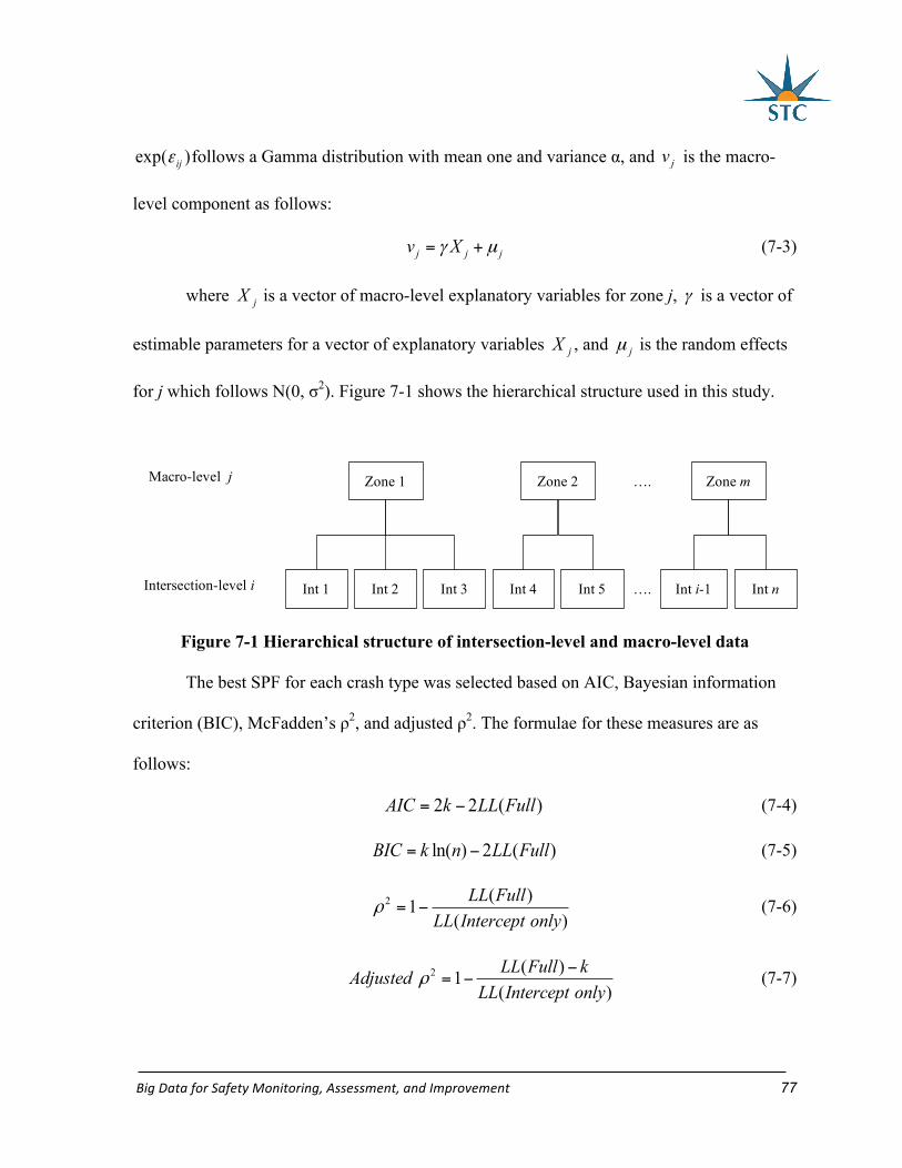
BigDataforSafetyMonitoring,Assessment,andImprovement 77
exp( )ijε follows a Gamma distribution with mean one and variance α, and jv is the macro-
level component as follows:
j j jv Xγ µ= + (7-3)
where jX is a vector of macro-level explanatory variables for zone j, γ is a vector of
estimable parameters for a vector of explanatory variables jX , and jµ is the random effects
for j which follows N(0, σ2). Figure 7-1 shows the hierarchical structure used in this study.
Figure 7-1 Hierarchical structure of intersection-level and macro-level data
The best SPF for each crash type was selected based on AIC, Bayesian information
criterion (BIC), McFadden’s ρ2, and adjusted ρ2. The formulae for these measures are as
follows:
2 2 ( )AIC k LL Full= − (7-4)
ln( ) 2 ( )BIC k n LL Full= − (7-5)
2 ( )1( )LL Full
LL Intercept onlyρ = − (7-6)
2 ( )1( )LL Full k
AdjustedLL Intercept only
ρ−
= − (7-7)
Int 1 Int 2 Int 3 Int 4 Int 5 Int i-1 Int n ….
Zone 1 Zone 2 Zone m …. Macro-level j
Intersection-level i

BigDataforSafetyMonitoring,Assessment,andImprovement 78
where k is number of parameters, n is the number of observations, ( )LL Full is the log-
likelihood for the full model, and ( )LL Intercept only is the log-likelihood for the intercept-
only model.
In order to prevent the multicollinearity problem, the models formed in this study do
not include highly correlated variables in the same model. The correlations between the
variables were checked by Spearman’s rank correlation method. If two variables were highly
correlated, they were not used simultaneously in the same model.
7.3 Macro-level Spatial Units
Varieties of spatial units have been used in macro-level studies. The spatial units
include census-based, traffic-based, or political boundaries. Figure 7-2 shows the examples of
various spatial units in the Orlando metropolitan area, Florida.
Census Block
A census block is the smallest geographic units used by the U.S. Bureau for the
collection and tabulation of decennial census data. However, detailed information of census
block is not available due to confidentiality requirement. On average, there are only 85 people
in one census block. Due to the lack of detailed information and extremely small sizes, census
blocks have not been used in this traffic safety studies.
Census Block Group (BG)
A census block group (BG) is the next level above the census block. A BG is
combinations of census blocks. Each BG contains about 39 census blocks on average.
Population in a BG ranges between 600 and 3,000 people. Some macroscopic traffic safety
studies adopted BGs as a base geographic unit (Levine et al., 1995, Abdel-Aty et al., 2013).
BigDataforSafetyMonitoring,Assessment,andImprovement 79
Traffic Analysis Zone (TAZ)
TAZs are special purpose geographic entities delineated by state and local
transportation officials for tabulating traffic-related data, especially journey-to-work and
place-of-work statistics (USCB, 2010). Since TAZs are the only traffic related zone system,
TAZs have been most popularly used in the macroscopic safety literature (Ladron de Guevara
et al., 2004; Lovegrove and Sayed, 2007; Hadayeghi et al., 2010; Naderan and Shahi, 2010;
Abdel-Aty et al., 2011; Wang et al., 2012; Abdel-Aty et al., 2013; Lee et al., 2014b, 2015b).
Census Tract (CT)
A census tract (CT) is designed to maintain homogenous socioeconomic status in a
zone. CTs are statistical sub-divisions of a county, and a CT may include 2,500 to 8,000
people. Several researchers have analyzed macroscopic traffic safety based on CTs (LaScala
et al., 2000; Wier et al., 2009; Ukkusuri et al., 2011).
ZIP-Code Tabulation Area (ZCTA)
ZIP code is the system of postal codes, it was created and used by the United States
Postal Service since 1963. In fact, ZIP codes are not a geographic unit but a collection of
mail delivery routes. U.S. Census Bureau created ZIP-Code Tabulation Areas (ZCTAs),
which are generalized areal representations of ZIP code service areas. ZCTA based data are
also provided from the U.S. Census Bureau. Many traffic safety studies using ZIP code have
been conducted (Stamatiadis and Puccini, 2000; Lee et al., 2014a; Lee et al., 2015a).
Traffic Analysis District (TAD)
Traffic analysis districts (TADs) are new; they are higher-level geographic entities for
traffic analysis (USCB, 2010). TADs are created by aggregating existing traffic analysis
zones. Traffic analysis districts may cross county boundaries, but they must nest within

BigDataforSafetyMonitoring,Assessment,andImprovement 80
MPOs. In recent, Abdel-Aty et al. (2016) developed macro-level safety models based on
TADs.
Census County Division (CCD)
Census county divisions (CCDs) are the statistical spatial units established
cooperatively by the U.S. Census Bureau and officials of state and local governments in 21
states. CCDs are designed to represent community areas, which focus on trading centers or
major land-use areas (USCB, 1994). No safety studies have been done using CCDs until this
point.
County
Counties are the primary administrative divisions for most states ((USCB, 1994). For
higher level of the macroscopic analysis, a county is also used as a geographic unit for the
macro-level study. Miaou et al. (2003), Noland and Oh (2004), Aguero-Valverde and Jovanis
(2006), and Huang et al. (2010) aggregated data into county-levels and analyzed crashes.

BigDataforSafetyMonitoring,Assessment,andImprovement 81
Census Block Group (BG) Traffic Analysis Zone (TAZ) Census Tract (CT) ZIP Code Tabulation Area
(ZCTA)
Traffic Analysis District (TAD) Census County Division (CCD) County Intersection locations
Figure 7-2 Various geographic units in Orlando metropolitan area, Florida
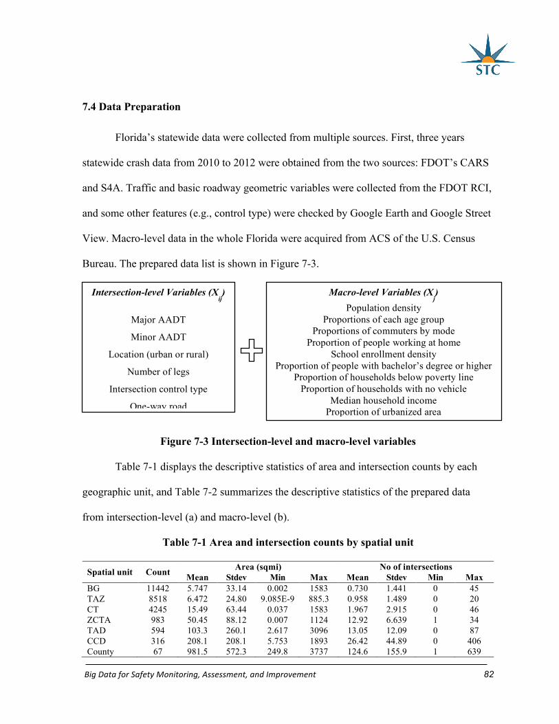
BigDataforSafetyMonitoring,Assessment,andImprovement 82
7.4 Data Preparation
Florida’s statewide data were collected from multiple sources. First, three years
statewide crash data from 2010 to 2012 were obtained from the two sources: FDOT’s CARS
and S4A. Traffic and basic roadway geometric variables were collected from the FDOT RCI,
and some other features (e.g., control type) were checked by Google Earth and Google Street
View. Macro-level data in the whole Florida were acquired from ACS of the U.S. Census
Bureau. The prepared data list is shown in Figure 7-3.
Figure 7-3 Intersection-level and macro-level variables
Table 7-1 displays the descriptive statistics of area and intersection counts by each
geographic unit, and Table 7-2 summarizes the descriptive statistics of the prepared data
from intersection-level (a) and macro-level (b).
Table 7-1 Area and intersection counts by spatial unit
Spatial unit Count Area (sqmi) No of intersections Mean Stdev Min Max Mean Stdev Min Max
BG 11442 5.747 33.14 0.002 1583 0.730 1.441 0 45 TAZ 8518 6.472 24.80 9.085E-9 885.3 0.958 1.489 0 20 CT 4245 15.49 63.44 0.037 1583 1.967 2.915 0 46 ZCTA 983 50.45 88.12 0.007 1124 12.92 6.639 1 34 TAD 594 103.3 260.1 2.617 3096 13.05 12.09 0 87 CCD 316 208.1 208.1 5.753 1893 26.42 44.89 0 406 County 67 981.5 572.3 249.8 3737 124.6 155.9 1 639
Intersection-level Variables (Xij)
Major AADT
Minor AADT
Location (urban or rural)
Number of legs
Intersection control type
One-way road
Macro-level Variables (Xj)
Population density Proportions of each age group
Proportions of commuters by mode Proportion of people working at home
School enrollment density Proportion of people with bachelor’s degree or higher
Proportion of households below poverty line Proportion of households with no vehicle
Median household income Proportion of urbanized area
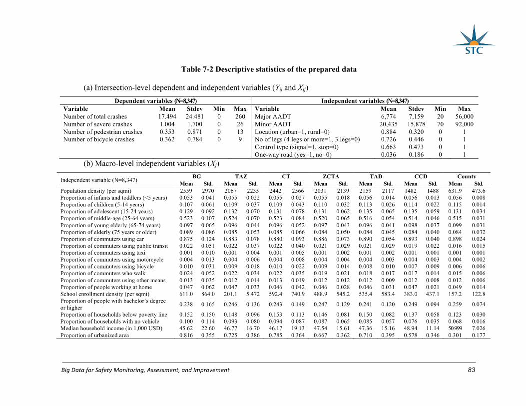
BigDataforSafetyMonitoring,Assessment,andImprovement 83
Table 7-2 Descriptive statistics of the prepared data
(a) Intersection-level dependent and independent variables (Yij and Xij) Dependent variables (N=8,347) Independent variables (N=8,347)
Variable Mean Stdev Min Max Variable Mean Stdev Min MaxNumber of total crashes 17.494 24.481 0 260 Major AADT 6,774 7,159 20 56,000Number of severe crashes 1.004 1.700 0 26 Minor AADT 20,435 15,878 70 92,000Number of pedestrian crashes 0.353 0.871 0 13 Location (urban=1, rural=0) 0.884 0.320 0 1Number of bicycle crashes 0.362 0.784 0 9 No of legs (4 legs or more=1, 3 legs=0) 0.726 0.446 0 1 Control type (signal=1, stop=0) 0.663 0.473 0 1 One-way road (yes=1, no=0) 0.036 0.186 0 1
(b) Macro-level independent variables (Xj)
Independent variable (N=8,347) BG TAZ CT ZCTA TAD CCD County Mean Std. Mean Std. Mean Std. Mean Std. Mean Std. Mean Std. Mean Std.
Population density (per sqmi) 2559 2970 2067 2235 2442 2566 2031 2139 2159 2117 1482 1488 631.9 473.6 Proportion of infants and toddlers (<5 years) 0.053 0.041 0.055 0.022 0.055 0.027 0.055 0.018 0.056 0.014 0.056 0.013 0.056 0.008 Proportion of children (5-14 years) 0.107 0.061 0.109 0.037 0.109 0.043 0.110 0.032 0.113 0.026 0.114 0.022 0.115 0.014 Proportion of adolescent (15-24 years) 0.129 0.092 0.132 0.070 0.131 0.078 0.131 0.062 0.135 0.065 0.135 0.059 0.131 0.034 Proportion of middle-age (25-64 years) 0.523 0.107 0.524 0.070 0.523 0.084 0.520 0.065 0.516 0.054 0.514 0.046 0.515 0.031 Proportion of young elderly (65-74 years) 0.097 0.065 0.096 0.044 0.096 0.052 0.097 0.043 0.096 0.041 0.098 0.037 0.099 0.031 Proportion of elderly (75 years or older) 0.089 0.086 0.085 0.053 0.085 0.066 0.084 0.050 0.084 0.045 0.084 0.040 0.084 0.032 Proportion of commuters using car 0.875 0.124 0.883 0.078 0.880 0.093 0.886 0.073 0.890 0.054 0.893 0.040 0.898 0.024 Proportion of commuters using public transit 0.022 0.051 0.022 0.037 0.022 0.040 0.021 0.029 0.021 0.029 0.019 0.022 0.016 0.015 Proportion of commuters using taxi 0.001 0.010 0.001 0.004 0.001 0.005 0.001 0.002 0.001 0.002 0.001 0.001 0.001 0.001 Proportion of commuters using motorcycle 0.004 0.013 0.004 0.006 0.004 0.008 0.004 0.004 0.004 0.003 0.004 0.003 0.004 0.002 Proportion of commuters using bicycle 0.010 0.031 0.009 0.018 0.010 0.022 0.009 0.014 0.008 0.010 0.007 0.009 0.006 0.006 Proportion of commuters who walk 0.024 0.052 0.022 0.034 0.022 0.035 0.019 0.021 0.018 0.017 0.017 0.014 0.015 0.006 Proportion of commuters using other means 0.013 0.035 0.012 0.014 0.013 0.019 0.012 0.012 0.012 0.009 0.012 0.008 0.012 0.006 Proportion of people working at home 0.047 0.062 0.047 0.033 0.046 0.042 0.046 0.028 0.046 0.031 0.047 0.021 0.049 0.014 School enrollment density (per sqmi) 611.0 864.0 201.1 5.472 592.4 740.9 488.9 545.2 535.4 583.4 383.0 437.1 157.2 122.8 Proportion of people with bachelor’s degree or higher 0.238 0.165 0.246 0.136 0.243 0.149 0.247 0.129 0.241 0.120 0.249 0.094 0.259 0.074
Proportion of households below poverty line 0.152 0.150 0.148 0.096 0.153 0.113 0.146 0.081 0.150 0.082 0.137 0.058 0.123 0.030 Proportion of households with no vehicle 0.100 0.114 0.093 0.080 0.094 0.087 0.087 0.065 0.085 0.057 0.076 0.035 0.068 0.016 Median household income (in 1,000 USD) 45.62 22.60 46.77 16.70 46.17 19.13 47.54 15.61 47.36 15.16 48.94 11.14 50.999 7.026 Proportion of urbanized area 0.816 0.355 0.725 0.386 0.785 0.364 0.667 0.362 0.710 0.395 0.578 0.346 0.301 0.177

BigDataforSafetyMonitoring,Assessment,andImprovement 84
7.5 Results and discussion
Three types of models were developed for each crash type as follows:
• Model Type (1): SPFs with micro-level variables only;
• Model Type (2): SPFs with micro-level variables and macro-level random-effects;
and
• Model Type (3): SPFs with micro-level variables and macro-level variables with
random-effects
Table 7-3 summarizes the goodness-of-fit measures of the developed models. There
are several findings from the model performances. Firstly, it was found that the models with
macro-level random-effects or variables outperform their counterpart without random-effects
(i.e., models with micro-level variables only). It is noteworthy that significant improvements
were observed by only adding macro-level random-effects. The AIC of the total crash SPF
with micro-level variables only is 54,862 whereas those of the SPFs with macro-level
random-effects only range between 53,336 and 54,554, which indicates a substantial
enhancement. Also, severe, pedestrian, and bicycle SPFs were enhanced only by adding
random-effects. Furthermore, the geographic units that provide the optimal data for
intersection SPFs were uncovered, in terms of AIC, BIC, ρ2, and Adjusted ρ2. The models
revealed that the total, severe, and bicycle crash SPF performs the best with ZCTA-based
data, and the pedestrian crash SPF showed the greatest performance with CT-based data.
Figure 7-4 compares adjusted ρ2 values of the SPFs with macro-level random-effects and
variables (Model Types (1) & (3)). From the results, it can be inferred that some geographic
units may be too small to aggregate meaningful shared characteristics between intersections
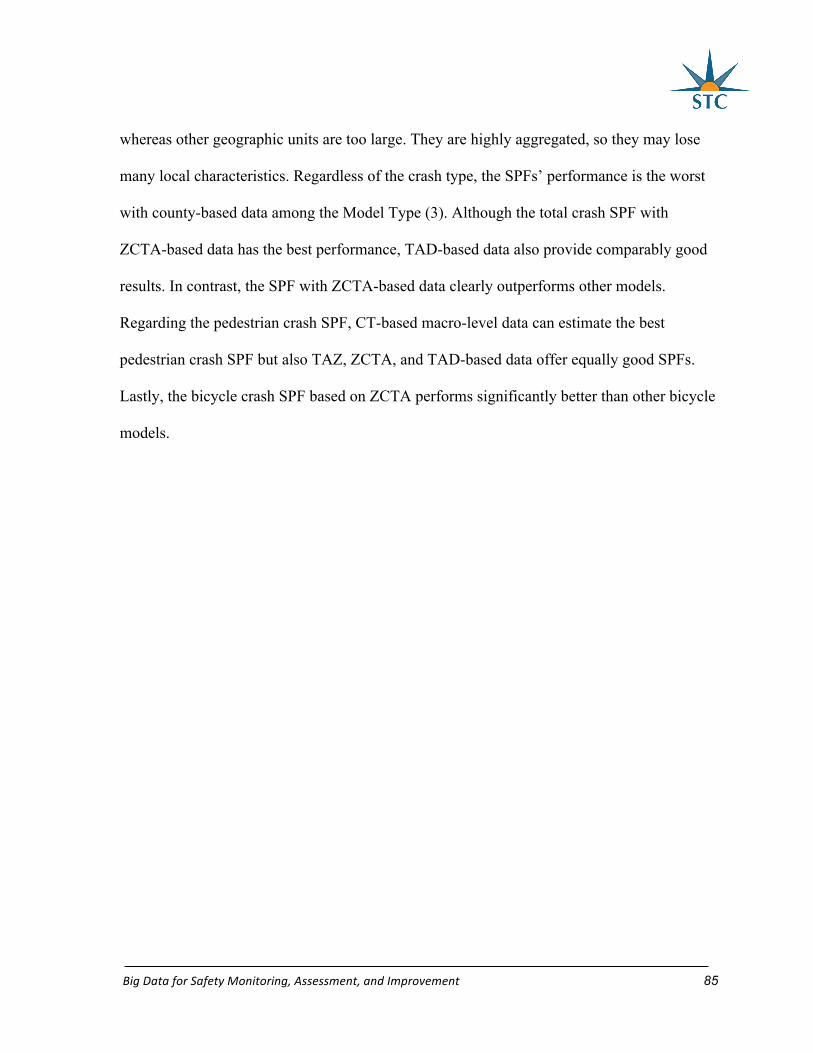
BigDataforSafetyMonitoring,Assessment,andImprovement 85
whereas other geographic units are too large. They are highly aggregated, so they may lose
many local characteristics. Regardless of the crash type, the SPFs’ performance is the worst
with county-based data among the Model Type (3). Although the total crash SPF with
ZCTA-based data has the best performance, TAD-based data also provide comparably good
results. In contrast, the SPF with ZCTA-based data clearly outperforms other models.
Regarding the pedestrian crash SPF, CT-based macro-level data can estimate the best
pedestrian crash SPF but also TAZ, ZCTA, and TAD-based data offer equally good SPFs.
Lastly, the bicycle crash SPF based on ZCTA performs significantly better than other bicycle
models.
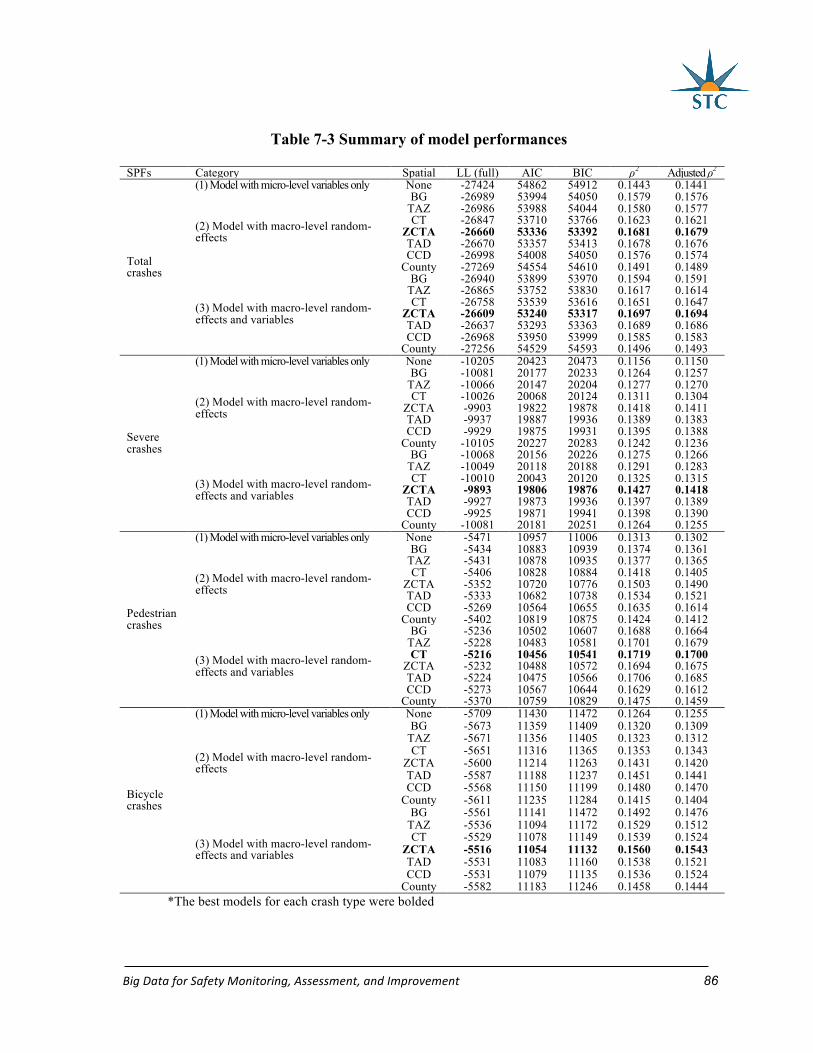
BigDataforSafetyMonitoring,Assessment,andImprovement 86
Table 7-3 Summary of model performances
SPFs Category Spatial LL (full) AIC BIC ρ2 Adjusted ρ2
Total crashes
(1) Model with micro-level variables only None -27424 54862 54912 0.1443 0.1441
(2) Model with macro-level random-effects
BG -26989 53994 54050 0.1579 0.1576 TAZ -26986 53988 54044 0.1580 0.1577 CT -26847 53710 53766 0.1623 0.1621
ZCTA -26660 53336 53392 0.1681 0.1679 TAD -26670 53357 53413 0.1678 0.1676 CCD -26998 54008 54050 0.1576 0.1574
County -27269 54554 54610 0.1491 0.1489
(3) Model with macro-level random-effects and variables
BG -26940 53899 53970 0.1594 0.1591 TAZ -26865 53752 53830 0.1617 0.1614 CT -26758 53539 53616 0.1651 0.1647
ZCTA -26609 53240 53317 0.1697 0.1694 TAD -26637 53293 53363 0.1689 0.1686 CCD -26968 53950 53999 0.1585 0.1583
County -27256 54529 54593 0.1496 0.1493
Severe crashes
(1) Model with micro-level variables only None -10205 20423 20473 0.1156 0.1150
(2) Model with macro-level random-effects
BG -10081 20177 20233 0.1264 0.1257 TAZ -10066 20147 20204 0.1277 0.1270 CT -10026 20068 20124 0.1311 0.1304
ZCTA -9903 19822 19878 0.1418 0.1411 TAD -9937 19887 19936 0.1389 0.1383 CCD -9929 19875 19931 0.1395 0.1388
County -10105 20227 20283 0.1242 0.1236
(3) Model with macro-level random-effects and variables
BG -10068 20156 20226 0.1275 0.1266 TAZ -10049 20118 20188 0.1291 0.1283 CT -10010 20043 20120 0.1325 0.1315
ZCTA -9893 19806 19876 0.1427 0.1418 TAD -9927 19873 19936 0.1397 0.1389 CCD -9925 19871 19941 0.1398 0.1390
County -10081 20181 20251 0.1264 0.1255
Pedestrian crashes
(1) Model with micro-level variables only None -5471 10957 11006 0.1313 0.1302
(2) Model with macro-level random-effects
BG -5434 10883 10939 0.1374 0.1361 TAZ -5431 10878 10935 0.1377 0.1365 CT -5406 10828 10884 0.1418 0.1405
ZCTA -5352 10720 10776 0.1503 0.1490 TAD -5333 10682 10738 0.1534 0.1521 CCD -5269 10564 10655 0.1635 0.1614
County -5402 10819 10875 0.1424 0.1412
(3) Model with macro-level random-effects and variables
BG -5236 10502 10607 0.1688 0.1664 TAZ -5228 10483 10581 0.1701 0.1679 CT -5216 10456 10541 0.1719 0.1700
ZCTA -5232 10488 10572 0.1694 0.1675 TAD -5224 10475 10566 0.1706 0.1685 CCD -5273 10567 10644 0.1629 0.1612
County -5370 10759 10829 0.1475 0.1459
Bicycle crashes
(1) Model with micro-level variables only None -5709 11430 11472 0.1264 0.1255
(2) Model with macro-level random-effects
BG -5673 11359 11409 0.1320 0.1309 TAZ -5671 11356 11405 0.1323 0.1312 CT -5651 11316 11365 0.1353 0.1343
ZCTA -5600 11214 11263 0.1431 0.1420 TAD -5587 11188 11237 0.1451 0.1441 CCD -5568 11150 11199 0.1480 0.1470
County -5611 11235 11284 0.1415 0.1404
(3) Model with macro-level random-effects and variables
BG -5561 11141 11472 0.1492 0.1476 TAZ -5536 11094 11172 0.1529 0.1512 CT -5529 11078 11149 0.1539 0.1524
ZCTA -5516 11054 11132 0.1560 0.1543 TAD -5531 11083 11160 0.1538 0.1521 CCD -5531 11079 11135 0.1536 0.1524
County -5582 11183 11246 0.1458 0.1444 *The best models for each crash type were bolded
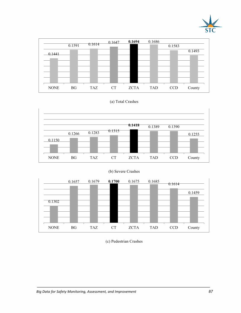
BigDataforSafetyMonitoring,Assessment,andImprovement 87
(a) Total Crashes
(b) Severe Crashes
(c) Pedestrian Crashes
0.1441
0.1591 0.1614 0.1647 0.1694 0.16860.1583
0.1493
NONE BG TAZ CT ZCTA TAD CCD County
0.11500.1266 0.1283 0.1315
0.1418 0.1389 0.1390
0.1255
NONE BG TAZ CT ZCTA TAD CCD County
0.1302
0.1657 0.1679 0.1700 0.1675 0.16850.1614
0.1459
NONE BG TAZ CT ZCTA TAD CCD County
BigDataforSafetyMonitoring,Assessment,andImprovement 88
(d) Bicycle Crashes
Figure 7-4 Comparison of adjusted ρ2 values of the SPFs with macro-level random-
effects and variables
Tables 7-4 to 7-7 display the modeling results for total, severe, pedestrian, and
bicycle crashes at intersections with macro-level variables. All the variables in the final
model are significant at the 5% confidence interval, and the following explanations are based
on the best model for each crash type.
7.5.1 Total Crash SPF
The best SPF of total crash was estimated with ZCTA-based data. Except for
‘Location (urban=1, rural=0)’ variable, all other intersection variables were statistically
significant at 5% in the SPF with ZCTA-based data. The location dummy variable was
highly correlated with ‘Log (population density)’ and thus these two variables could not be
used at the same time. These variables were attempted one by one and the model with ‘Log
(population density)’ outperforms the one with the location variable. Both ‘Log (major
AADT)’ and ‘Log (minor AADT)’ were used as exposure variables and as expected they had
positive and significant impacts on total crashes at intersections. The major AADT had a
greater impact than the minor AADT as the major AADT had a larger coefficient. It was also
0.1255
0.1476 0.1512 0.1524 0.1543 0.1521 0.15240.1444
NONE BG TAZ CT ZCTA TAD CCD County

BigDataforSafetyMonitoring,Assessment,andImprovement 89
confirmed by previous studies (AASHTO, 2010; Jonsson et al., 2009). This phenomenon is
also observed in all other models (i.e., severe, pedestrian, and bicycle crash SPFs).
Meanwhile, ‘No of legs (4 legs or more=1, 3 legs=0)’, ‘Control type (signal=1, stop=0)’, and
‘One-way road (yes=1, no=0)’ were positively related with total crashes. The intersections
with more legs have more conflict points that result in more crashes. Regarding the
signalization, it may reduce some types of crashes (i.e., angle); however, existing studies has
proven that the signalization significantly increase other types of crashes (i.e., rear-end).
Thus, the overall crash counts may increase due to the signalization. It was also shown the
intersections with one-way road tend to have more crashes. It may be because one-way roads
may confuse the drivers who are not familiar with the one-way road operation, especially at
intersections.
‘Log (population density)’ was positively related to total crash counts (Ladron de
Guevara et al., 2004, Lovegrove and Sayed, 2007; Lee et al., 2014b). Ladron de Guevara et
al. (2004) explained that population density reflects the degree of interaction among people;
therefore, the areas with larger population density may result in greater interactions and
conflicts. ‘Proportion of elderly (75 years or older)’ has a negative effect on total crash
counts, which is consistent with several prior studies (Lee et al., 2014a; Huang et al., 2010).
It may be explained by the degree of exposure. Lee et al. (2014a) claimed that elderly drivers
are less exposed to traffic crashes because they have much shorter trip lengths compared to
other age groups. Furthermore, median household income (in $1,000) was negatively
associated with total crash counts, which implies that the area with lower income households
has a propensity to experience more crashes at intersections (Lee et al., 2014a; Huang et al.,
2010). Lee et al. (2014a) and Martinez and Veloz (1996) explained that people from lower-
BigDataforSafetyMonitoring,Assessment,andImprovement 90
income areas are not able to afford to purchase newer and safer vehicle or equipment, and
have less chance to get traffic safety information. Therefore, they are more likely to be
involved in traffic crashes. Lastly, ‘Proportion of commuters using public transit’ has a
positive effect on total crashes. The zones with higher public transit use are often located in
highly urbanized area with concentrated activities; and thus they are likely to experience
more crashes (Abdel-Aty et al., 2013; Lee et al., 2013).
7.5.2 Severe Crash SPF
Again, the severe crash SPF performed the best with ZCTA-based data. Almost all
intersection-level variables were significant in the SPF with ZCTA-based data. ‘Location
(urban=1, rural=0)’ is significant and negatively associated with severe crashes. It infers that
more severe crashes occur at rural intersections, compared to urban intersections. At this
time, the SPF with the location dummy variable performs better than that with ‘Log
(population density)’. ‘One-way road (yes=1, no=0)’ was not significant for severe crashes.
The other intersection-level variables are consistent with the total crash SPF. Three ZCTA-
based variables were found significant. ‘Proportion of commuters using motorcycle’ had a
positive coefficient whereas ‘Proportion of commuters who walk’ and ‘Median household
income (in $1,000)’ had a negative coefficient in the severe crash SPF. The motorcycle
variable showed that the intersections within the area with higher proportion of motorcycle
using commuters had more severe crashes (WHO, 2013). On the other hand, the intersections
with more walking commuters had a propensity to experience less severe crashes. It may be
because the areas with higher proportion of walking commuters are in urbanized areas with
possibly lower speed limit. The income variable is in line with that in the total crash SPF.

BigDataforSafetyMonitoring,Assessment,andImprovement 91
7.5.3 Pedestrian Crash SPF
The optimal macro-level data for the pedestrian crash SPF is CT-based data. The
intersection-level variables including ‘Log (major AADT)’, ‘Log (minor AADT)’, ‘No of
legs (4 legs or more=1, 3 legs=0)’, and ‘Control type (signal=1, stop=0)’ have a positive
relationship with pedestrian crashes. Overall six CT-based variables were statistically
significant. ‘Log (population density)’, ‘Proportion of commuters using public transit’, and
‘Proportion of commuters who walk’ are positively while ‘Proportion of adolescent (15-24
years)’, ‘Proportion of elderly (75 years or older)’, and ‘Median household income (in
$1,000)’ are negatively related with pedestrian crash counts. The three CT-based variables
with positive effects may be a good surrogate exposure variable for pedestrian crashes. In
Model Type (1), there is no exposure variable for pedestrians but only traffic volume;
therefore, the pedestrian crash model could be significantly improved by including the
macro-level variables including the surrogate exposure variables explained above. Regarding
to the public transit using and walking commuters, they are pedestrians when they access to
public transportation facilities or to workplace (e.g., bus stop or rail station) by walking
(Abdel-Aty et al., 2013). Lastly, the areas with both adolescent and elderly people have less
pedestrian crashes, which hint at that these people are less exposed to pedestrian crashes
compared to other age groups (e.g., middle age).
7.5.4 Bicycle Crash SPF
The preeminent bicycle SPF was developed with ZCTA-based data. The significance
of the intersection-variables is the same as those in the pedestrian crash SPF. Five ZCTA-
based variables were found significant for bicycle crashes. ‘Log (population density)’,

BigDataforSafetyMonitoring,Assessment,andImprovement 92
‘Proportion of motorcycle’, and ‘Proportion of commuters using bicycle’ have a positive
while ‘Proportion of adolescent’ and ‘Median household income (in $1,000)’ have a negative
relation with bicycle crashes. The population density and the bicycle commuter variables
were as expected but it is interesting that the motorcycle commuter variable also has a
positive effect. It is thought that there are common features in motorcycle and bicycle use.
Both transportation modes are used for recreational and leisure activities. Therefore, the
communities with the larger number of bicyclists also may have more motorcyclists. Similar
to the pedestrian crash SPF, the model has been significantly improved by adding macro-
level variables (i.e., population density, bicycle/motorcycle using commuter variables)
compared to the model with intersection-level variables only.
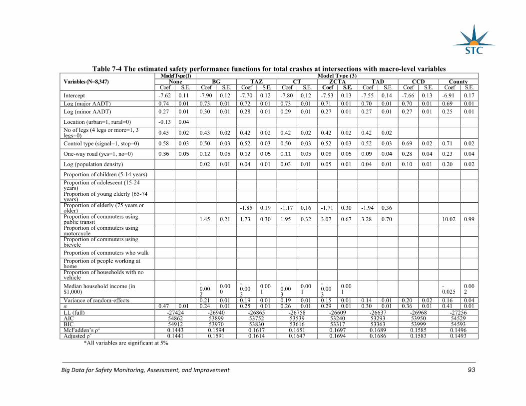
BigDataforSafetyMonitoring,Assessment,andImprovement 93
Table 7-4 The estimated safety performance functions for total crashes at intersections with macro-level variables
Variables (N=8,347) Model Type (1) Model Type (3)
None BG TAZ CT ZCTA TAD CCD County Coef S.E. Coef S.E. Coef S.E. Coef S.E. Coef S.E. Coef S.E. Coef S.E. Coef S.E.
Intercept -7.62 0.11 -7.90 0.12 -7.70 0.12 -7.80 0.12 -7.53 0.13 -7.55 0.14 -7.66 0.13 -6.91 0.17 Log (major AADT) 0.74 0.01 0.73 0.01 0.72 0.01 0.73 0.01 0.71 0.01 0.70 0.01 0.70 0.01 0.69 0.01 Log (minor AADT) 0.27 0.01 0.30 0.01 0.28 0.01 0.29 0.01 0.27 0.01 0.27 0.01 0.27 0.01 0.25 0.01
Location (urban=1, rural=0) -0.13 0.04 No of legs (4 legs or more=1, 3 legs=0) 0.45 0.02 0.43 0.02 0.42 0.02 0.42 0.02 0.42 0.02 0.42 0.02
Control type (signal=1, stop=0) 0.58 0.03 0.50 0.03 0.52 0.03 0.50 0.03 0.52 0.03 0.52 0.03 0.69 0.02 0.71 0.02
One-way road (yes=1, no=0) 0.36 0.05 0.12 0.05 0.12 0.05 0.11 0.05 0.09 0.05 0.09 0.04 0.28 0.04 0.23 0.04
Log (population density) 0.02 0.01 0.04 0.01 0.03 0.01 0.05 0.01 0.04 0.01 0.10 0.01 0.20 0.02
Proportion of children (5-14 years) Proportion of adolescent (15-24 years) Proportion of young elderly (65-74 years) Proportion of elderly (75 years or older) -1.85 0.19 -1.17 0.16 -1.71 0.30 -1.94 0.36 Proportion of commuters using public transit 1.45 0.21 1.73 0.30 1.95 0.32 3.07 0.67 3.28 0.70 10.02 0.99 Proportion of commuters using motorcycle Proportion of commuters using bicycle
Proportion of commuters who walk Proportion of people working at home Proportion of households with no vehicle
Median household income (in $1,000)
-0.002
0.000
-0.003
0.001
-0.003
0.001
-0.003
0.001 -
0.025 0.002
Variance of random-effects 0.21 0.01 0.19 0.01 0.19 0.01 0.15 0.01 0.14 0.01 0.20 0.02 0.16 0.04 α 0.47 0.01 0.24 0.01 0.25 0.01 0.26 0.01 0.29 0.01 0.30 0.01 0.36 0.01 0.41 0.01 LL (full) -27424 -26940 -26865 -26758 -26609 -26637 -26968 -27256 AIC 54862 53899 53752 53539 53240 53293 53950 54529 BIC 54912 53970 53830 53616 53317 53363 53999 54593 McFadden’s ρ2 0.1443 0.1594 0.1617 0.1651 0.1697 0.1689 0.1585 0.1496 Adjusted ρ2 0.1441 0.1591 0.1614 0.1647 0.1694 0.1686 0.1583 0.1493
*All variables are significant at 5%
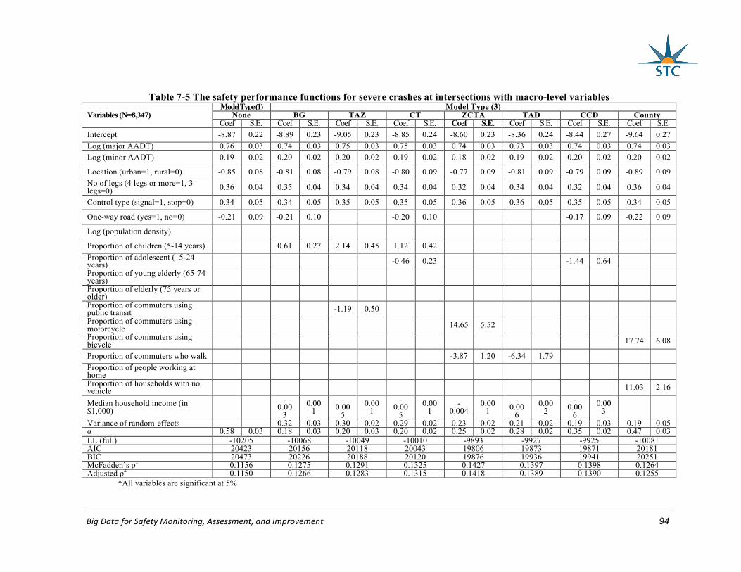
BigDataforSafetyMonitoring,Assessment,andImprovement 94
Table 7-5 The safety performance functions for severe crashes at intersections with macro-level variables
Variables (N=8,347) Model Type (1) Model Type (3)
None BG TAZ CT ZCTA TAD CCD County Coef S.E. Coef S.E. Coef S.E. Coef S.E. Coef S.E. Coef S.E. Coef S.E. Coef S.E.
Intercept -8.87 0.22 -8.89 0.23 -9.05 0.23 -8.85 0.24 -8.60 0.23 -8.36 0.24 -8.44 0.27 -9.64 0.27 Log (major AADT) 0.76 0.03 0.74 0.03 0.75 0.03 0.75 0.03 0.74 0.03 0.73 0.03 0.74 0.03 0.74 0.03 Log (minor AADT) 0.19 0.02 0.20 0.02 0.20 0.02 0.19 0.02 0.18 0.02 0.19 0.02 0.20 0.02 0.20 0.02
Location (urban=1, rural=0) -0.85 0.08 -0.81 0.08 -0.79 0.08 -0.80 0.09 -0.77 0.09 -0.81 0.09 -0.79 0.09 -0.89 0.09 No of legs (4 legs or more=1, 3 legs=0) 0.36 0.04 0.35 0.04 0.34 0.04 0.34 0.04 0.32 0.04 0.34 0.04 0.32 0.04 0.36 0.04
Control type (signal=1, stop=0) 0.34 0.05 0.34 0.05 0.35 0.05 0.35 0.05 0.36 0.05 0.36 0.05 0.35 0.05 0.34 0.05
One-way road (yes=1, no=0) -0.21 0.09 -0.21 0.10 -0.20 0.10 -0.17 0.09 -0.22 0.09
Log (population density)
Proportion of children (5-14 years) 0.61 0.27 2.14 0.45 1.12 0.42 Proportion of adolescent (15-24 years) -0.46 0.23 -1.44 0.64 Proportion of young elderly (65-74 years) Proportion of elderly (75 years or older) Proportion of commuters using public transit -1.19 0.50 Proportion of commuters using motorcycle 14.65 5.52 Proportion of commuters using bicycle 17.74 6.08
Proportion of commuters who walk -3.87 1.20 -6.34 1.79 Proportion of people working at home Proportion of households with no vehicle 11.03 2.16
Median household income (in $1,000)
-0.00
3 0.00
1 -
0.005
0.001
-0.00
5 0.00
1 -
0.004 0.00
1 -
0.006
0.002
-0.00
6 0.00
3
Variance of random-effects 0.32 0.03 0.30 0.02 0.29 0.02 0.23 0.02 0.21 0.02 0.19 0.03 0.19 0.05 α 0.58 0.03 0.18 0.03 0.20 0.03 0.20 0.02 0.25 0.02 0.28 0.02 0.35 0.02 0.47 0.03 LL (full) -10205 -10068 -10049 -10010 -9893 -9927 -9925 -10081 AIC 20423 20156 20118 20043 19806 19873 19871 20181 BIC 20473 20226 20188 20120 19876 19936 19941 20251 McFadden’s ρ2 0.1156 0.1275 0.1291 0.1325 0.1427 0.1397 0.1398 0.1264 Adjusted ρ2 0.1150 0.1266 0.1283 0.1315 0.1418 0.1389 0.1390 0.1255
*All variables are significant at 5%
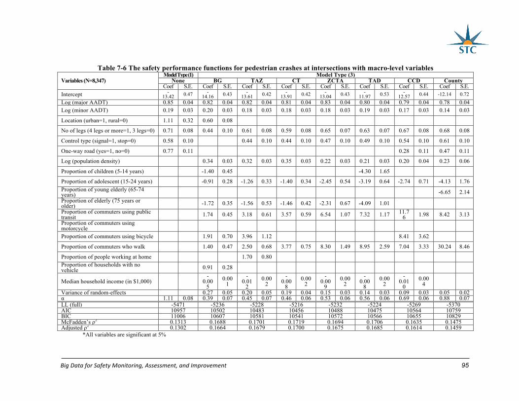
BigDataforSafetyMonitoring,Assessment,andImprovement 95
Table 7-6 The safety performance functions for pedestrian crashes at intersections with macro-level variables
Variables (N=8,347) Model Type (1) Model Type (3)
None BG TAZ CT ZCTA TAD CCD County Coef S.E. Coef S.E. Coef S.E. Coef S.E. Coef S.E. Coef S.E. Coef S.E. Coef S.E.
Intercept -13.42 0.47 -
14.16 0.43 -13.61 0.42 -
13.91 0.42 -13.04 0.43 -
11.97 0.53 -12.57 0.44 -12.14 0.72
Log (major AADT) 0.85 0.04 0.82 0.04 0.82 0.04 0.81 0.04 0.83 0.04 0.80 0.04 0.79 0.04 0.78 0.04 Log (minor AADT) 0.19 0.03 0.20 0.03 0.18 0.03 0.18 0.03 0.18 0.03 0.19 0.03 0.17 0.03 0.14 0.03
Location (urban=1, rural=0) 1.11 0.32 0.60 0.08
No of legs (4 legs or more=1, 3 legs=0) 0.71 0.08 0.44 0.10 0.61 0.08 0.59 0.08 0.65 0.07 0.63 0.07 0.67 0.08 0.68 0.08
Control type (signal=1, stop=0) 0.58 0.10 0.44 0.10 0.44 0.10 0.47 0.10 0.49 0.10 0.54 0.10 0.61 0.10
One-way road (yes=1, no=0) 0.77 0.11 0.28 0.11 0.47 0.11
Log (population density) 0.34 0.03 0.32 0.03 0.35 0.03 0.22 0.03 0.21 0.03 0.20 0.04 0.23 0.06
Proportion of children (5-14 years) -1.40 0.45 -4.30 1.65
Proportion of adolescent (15-24 years) -0.91 0.28 -1.26 0.33 -1.40 0.34 -2.45 0.54 -3.19 0.64 -2.74 0.71 -4.13 1.76 Proportion of young elderly (65-74 years) -6.65 2.14 Proportion of elderly (75 years or older) -1.72 0.35 -1.56 0.53 -1.46 0.42 -2.31 0.67 -4.09 1.01 Proportion of commuters using public transit 1.74 0.45 3.18 0.61 3.57 0.59 6.54 1.07 7.32 1.17 11.7
6 1.98 8.42 3.13 Proportion of commuters using motorcycle
Proportion of commuters using bicycle 1.91 0.70 3.96 1.12 8.41 3.62
Proportion of commuters who walk 1.40 0.47 2.50 0.68 3.77 0.75 8.30 1.49 8.95 2.59 7.04 3.33 30.24 8.46
Proportion of people working at home 1.70 0.80 Proportion of households with no vehicle 0.91 0.28
Median household income (in $1,000) -
0.005
0.001
-0.01
2 0.00
2 -
0.008
0.002
-0.00
9 0.00
2 -
0.008
0.002
-0.01
0 0.00
4
Variance of random-effects 0.27 0.05 0.20 0.05 0.19 0.04 0.15 0.03 0.14 0.03 0.09 0.03 0.05 0.02 α 1.11 0.08 0.39 0.07 0.45 0.07 0.46 0.06 0.53 0.06 0.56 0.06 0.69 0.06 0.88 0.07 LL (full) -5471 -5236 -5228 -5216 -5232 -5224 -5269 -5370 AIC 10957 10502 10483 10456 10488 10475 10564 10759 BIC 11006 10607 10581 10541 10572 10566 10655 10829 McFadden’s ρ2 0.1313 0.1688 0.1701 0.1719 0.1694 0.1706 0.1635 0.1475 Adjusted ρ2 0.1302 0.1664 0.1679 0.1700 0.1675 0.1685 0.1614 0.1459
*All variables are significant at 5%
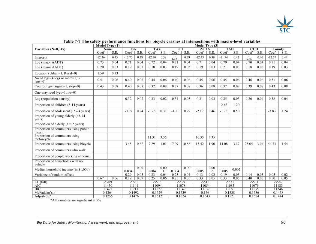
BigDataforSafetyMonitoring,Assessment,andImprovement 96
Table 7-7 The safety performance functions for bicycle crashes at intersections with macro-level variables
Variables (N=8,347) Model Type (1) Model Type (3)
None BG TAZ CT ZCTA TAD CCD County Coef S.E. Coef S.E. Coef S.E. Coef S.E. Coef S.E. Coef S.E. Coef S.E. Coef S.E.
Intercept -12.36 0.45 -12.75 0.38 -12.70 0.38 -12.81 0.39 -12.43 0.39 -11.74 0.42 -
12.47 0.40 -12.67 0.44 Log (major AADT) 0.73 0.04 0.71 0.04 0.72 0.04 0.71 0.04 0.71 0.04 0.70 0.04 0.70 0.04 0.71 0.04 Log (minor AADT) 0.20 0.03 0.19 0.03 0.18 0.03 0.19 0.03 0.19 0.03 0.21 0.03 0.18 0.03 0.19 0.03
Location (Urban=1, Rural=0) 1.59 0.33 No of legs (4 legs or more=1, 3 legs=0) 0.51 0.06 0.40 0.06 0.44 0.06 0.40 0.06 0.45 0.06 0.45 0.06 0.46 0.06 0.51 0.06
Control type (signal=1, stop=0) 0.43 0.08 0.40 0.08 0.32 0.08 0.37 0.08 0.36 0.08 0.37 0.08 0.39 0.08 0.43 0.08
One-way road (yes=1, no=0)
Log (population density) 0.32 0.02 0.33 0.02 0.34 0.03 0.31 0.03 0.25 0.03 0.26 0.04 0.38 0.04
Proportion of children (5-14 years) -2.63 1.20
Proportion of adolescent (15-24 years) -0.65 0.24 -1.28 0.31 -1.11 0.29 -2.19 0.46 -1.78 0.50 -3.83 1.24 Proportion of young elderly (65-74 years)
Proportion of elderly (>=75 years) Proportion of commuters using public transit Proportion of commuters using motorcycle 11.31 3.55 16.35 7.35
Proportion of commuters using bicycle 3.45 0.62 7.29 1.01 7.09 0.88 13.42 1.90 14.08 3.17 25.05 3.04 44.73 4.54
Proportion of commuters who walk
Proportion of people working at home Proportion of households with no vehicle
Median household income (in $1,000) -0.004
0.001
-0.004
0.001
-0.004
0.001
-0.005
0.002
-0.005 0.002
Variance of random-effects 0.29 0.05 0.23 0.04 0.23 0.04 0.13 0.02 0.19 0.03 0.14 0.03 0.05 0.02 α 0.67 0.06 0.19 0.07 0.25 0.06 0.25 0.05 0.33 0.05 0.33 0.05 0.40 0.05 0.50 0.05 LL (full) -5709 -5561 -5536 -5529 -5516 -5531 -5531 -5582 AIC 11430 11141 11094 11078 11054 11083 11079 11183 BIC 11472 11211 11172 11149 11132 11160 11135 11246 McFadden’s ρ2 0.1264 0.1492 0.1529 0.1539 0.156 0.1538 0.1536 0.1458 Adjusted ρ2 0.1255 0.1476 0.1512 0.1524 0.1543 0.1521 0.1524 0.1444
*All variables are significant at 5%
BigDataforSafetyMonitoring,Assessment,andImprovement 97
7.6 Summary
The SPFs play an important role in traffic safety as they are used to identify hotspots
and assess the effectiveness of safety treatments. Numerous SPFs have been developed but
most of them are based on the micro-level (i.e., intersection, segment, and corridor). Some
researchers have analyzed crashes at the macro-level, but few studies have attempted to
combine micro-level with macro-level data for developing SPFs.
This chapter aimed at answering the three research questions: (1) can intersection
SPFs be improved by considering macro-level geographic units? (2) what would be the best
spatial unit for the SPFs? and (3) what macro-level factors do have significant effects on
intersection crashes? In order to answer these questions, traffic, geometric, and crash data for
Florida’s major intersections (N=8,347) were collected from the FDOT and Google Earth.
Demographic, socioeconomic, and commute data were obtained from the ACS of the U.S.
Census Bureau. The intersection-level data were combined with macro-level data from seven
spatial units (i.e., BG, TAZ, CT, ZCTA, TAD, CCD, and county). A series of mixed-effects
negative binomial models were developed for total, severe, pedestrian, and bicycle crashes
with the intersection-level data merged with the macro-level data from the various
geographic units mentioned above. The modeling results revealed the following key findings:
• The SPFs with macro-level random-effects only and those with both macro-level
random effects and variables outperform those only with intersection-level variables.
• The intersection SPFs can be considerably augmented by only including macro-
level random-effects.

BigDataforSafetyMonitoring,Assessment,andImprovement 98
• The intersection SPFs for total, severe, and bicycle crash SPFs have the greatest
performance with ZCTA-based data.
• The intersection SPF for pedestrian crashes performs the best with CT-based data.
The results imply that generally medium-sized geographic units (i.e., ZCTA and CT)
work well for intersection-level SPFs. It is because some spatial units (e.g., BG and TAZ)
may be too small to aggregate meaningful shared characteristics between intersections;
whereas, other geographic units (e.g., county) are excessively highly aggregated and miss
much local information.
Furthermore, the modeling results revealed that the following macro-level variables
are significant:
• The population density has a positive relationship with total, pedestrian, and bicycle
crashes;
• The proportion of young (15-24 years) group is negatively related to pedestrian and
bicycle crashes;
• Elderly (75 years or older) age group are less exposed to total and pedestrian
crashes;
• The proportion of public transit using commuters has a positive relationship with
total and pedestrian crashes;
• The proportion of motorcycle using commuters is positively associated to severe
and bicycle crashes;
• The proportion of bicycle using commuters has a positive effect on bicycle crashes;
• The proportion of walking commuters has a negative effect for severe crashes while
it has a positive effect for pedestrian crashes;
BigDataforSafetyMonitoring,Assessment,andImprovement 99
• The median household income is negatively associated with four types of crashes.
Both pedestrian and bicycle crash SPFs have been significantly enhanced with macro-
level variables compared to that with intersection-level variables only. This is because there
is no exposure variable for pedestrians and bicyclists but only traffic volume. The significant
improvements of the pedestrian and bicycle crash SPFs imply that some macro-level
variables such as population density, walking and bicycling commuter variables function as a
good surrogate exposure variable. It is concluded that the performance of micro-SPFs can be
considerably augmented with the proposed hierarchical modeling methodology in this study.
There are several possible extensions to this study. First, segment-level SPFs with
macro-level variables can be estimated. It is possible that the optimal geographic unit for
segment traffic safety estimation differs from the intersection-level SPFs. Second, it will be
necessary to apply the data from different regions and check if the results from this study are
valid in other states.
BigDataforSafetyMonitoring,Assessment,andImprovement 100
CHAPTER8:CONCLUSIONS
Now more than ever more information is collected, stored, and processed. The large
amount of information, characterized by variety, volume, velocity, variability, complexity,
and value, is defined as big data. In return, the big data have brought about enormous
benefits and challenges to human life. As an important aspect of human life, the
transportation field has also generated big data. In turn, implementing the transportation
related big data to monitor, assess, and improve traffic safety is the focus of this study.
Four types of data were collected and integrated to explore crash contributing factors
with the aim of improving traffic safety. They are crash, traffic, road geometric, and
macroscopic data. Each type of data was from several sources, and different sources were
combined to give information that is more complete. The crash data were from CARS and
S4A. CARS provides more detailed crash information than S4A, and S4A records more
crash. The traffic data were from AVI and MVDS. AVI sensors provide traffic information
for roadway segments: travel time and space mean speed for each vehicle. On the other hand,
MVDS detectors are point-based and provide vehicle count, time mean speed, lane
occupancy for each lane at 1-minute intervals for each point. Road geometric data were from
RCI, which is maintained by FDOT, or manually collected. RCI dataset offer 323 road
geometric characteristics for each roadway segment in Florida. However, some geometric
parameters are specific to a roadway type and cannot find in RCI, for example weaving
segment length. Thus, these geometric data were manually collected from ArcGIS map.
Microscopic data were from the FDOT Central Office and the ACS of the U.S. Census
BigDataforSafetyMonitoring,Assessment,andImprovement 101
Bureau. These data reflect the behaviors of traffic participants, such as pedestrian, bicyclist,
and driver.
After processing and integrating the data above, preliminary safety evaluation has
been conducted by data visualization. Hourly volume distribution was described by three-
dimension spatio-temporal and contour plots. The expressway congestion was pictured and
was measured using TTI, occupancy, and CI based on AVI and MVDS traffic data.
Subsequently, the spatial patterns of traffic crashes by facility types were visualized from
2011 to 2014. The visualization of crashes enabled researchers to easily detect crash hotspots
and suggest appropriate engineering countermeasures.
Then, the big traffic data were used to build a microscopic simulation network for
expressway weaving segments, which have a higher crash potential than other expressway
mainline segments. The input big traffic data made the simulation network well calibrated
and validated, because the simulated volume, speed, and safety were highly consistent with
those of the field. Furthermore, two conflict prediction models were estimated using the
traffic data from VISSIM simulation and conflict information from SSAM. One model was
based on a 5-minute intervals and the other was based on a 1-minute intervals. In both
models, Logarithm of vehicle count, maximum influence length, and average acceleration at
the beginning of weaving segment were significant variables. The model performance of the
1-minute interval model was better than that of the 5-minute interval model by providing
higher AUCs and lower standard deviation of variable coefficients.
Reduced travel time reliability could cause unstable traffic flow thus affects traffic
safety. This study separately estimated SV and MV crash frequencies using three travel time
reliability indicators: Percent Variation, Buffer Index, and Misery Index. The results showed

BigDataforSafetyMonitoring,Assessment,andImprovement 102
that Buffer Index and Misery Index had significant positive impact on MV crash frequency;
however, Percent Variation was not significant in MV crash frequency model. On the other
hand, all indicators were not significantly related to SV crash frequency. Additionally,
Percent Variation was used in real-time safety analysis to estimate MV crash potential given
a crash occurrence. The model indicates that high Percent Variation would significantly
increase MV crash risk.
The safety of a roadway facility is not only determined by the facility’s geometric
design and traffic, but also it might be impacted by the macroscopic characteristics of the
zone, which the facility lies in. Macroscopic parameters were implemented in real-time crash
analysis for expressway ramps and crash frequency estimation for intersections. In the real-
time crash analysis for ramps, land-use and trip generation parameters were important crash
contributing factors. Two SVM models were applied to predict crash occurrence: one with all
variables and the other only with significant variables identified by a logistic regression
model. The SVM with all variables had an overfitting issue. It is recommended to integrate
data mining method and traditional statistical model to alleviate overfitting issue and to
improve model performance.
In the crash frequency prediction for intersections, both pedestrian and bicycle crash
SPFs have been significantly enhanced with macro-level variables compared to that with
intersection-level variables only. The significant improvements of the pedestrian and bicycle
crash SPFs imply that some macro-level variables such as population density, walking and
bicycling commuter variables function as a good surrogate exposure variable. Additionally,
total and severe crash SPFs were also improved by adding macro-level random effects and
variables. The results also indicated that medium-sized geographic units (i.e., ZCTA and CT)

BigDataforSafetyMonitoring,Assessment,andImprovement 103
might work better for intersection-level SPFs than other macro-level spatial units. Since,
macro-level data are easily accessible from the U.S. Census Bureau, it is strongly
recommended to incorporate macro-level data in developing micro-level SPFs.
BigDataforSafetyMonitoring,Assessment,andImprovement 104
REFERENCES
AASHTO, 2010. Highway safety manual. American Association of State Highway and Transportation Officials, Washington D.C.
Abdel-Aty, M., Lee J., Eluru N., Cai Q., Al Amili S., Alarifi S., 2016. Enhancing and Generalizing the Two-Level Screening Approach Incorporating the Highway Safety Manual (HSM) Methods, Phase 2 report.
Abdel-Aty, M., Lee, J., Siddiqui, C., Choi, K., 2013. Geographical unit based analysis in the context of transportation safety planning. Transportation Research Part A: Policy and Practice 49, 62-75.
Abdel-Aty, M., Pande, A., 2005. Identifying crash propensity using specific traffic speed conditions. Journal of Safety Research 36 (1), 97-108.
Abdel-Aty, M., Pemmanaboina, R., 2006. Calibrating a real-time traffic crash-prediction model using archived weather and its traffic data. Intelligent Transportation Systems, IEEE Transactions on Intelligent Transportation System 7 (2), 167-174.
Abdel-Aty, M., Siddiqui, C., Huang, H., Wang, X., 2011. Integrating trip and roadway characteristics to manage safety in traffic analysis zones. Transportation Research Record: Journal of the Transportation Research Board (2213), 20-28.
Abdel-Aty, M., Uddin, N., Pande, A., Abdalla, F., Hsia, L., 2004. Predicting freeway crashes from loop detector data by matched case-control logistic regression. Transportation Research Record: Journal of the Transportation Research Board (1897), 88-95.
Aguero-Valverde, J., Jovanis, P.P., 2006. Spatial analysis of fatal and injury crashes in pennsylvania. Accident Analysis & Prevention 38 (3), 618-625.
Ahmed, M., Huang, H., Abdel-Aty, M., Guevara, B., 2011. Exploring a bayesian hierarchical approach for developing safety performance functions for a mountainous freeway. Accident Analysis & Prevention 43 (4), 1581-1589.
Autey, J., Sayed, T., Zaki, M.H., 2012. Safety evaluation of right-turn smart channels using automated traffic conflict analysis. Accident Analysis & Prevention 45, 120-130.
Breiman, L., 2001. Random forests. Machine learning 45 (1), 5-32.
Cafiso, S., Garcia, A., Cavarra, R., 2011. Before-and-after study of crosswalks using pedestrian risk index. In: Proceedings of the Transportation Research Board 90th Annual Meeting. Washington, D.C.
Cambridge Systematics, Inc., 2004. Traffic congestion and reliability: Trends and advanced strategies for congestion mitigation. Federal Highway Administration report
BigDataforSafetyMonitoring,Assessment,andImprovement 105
Campbell, C., Ying, Y., 2011. Learning with support vector machines. Synthesis lectures on artificial intelligence and machine learning 5 (1), 1-95.
Deng, N., Tian, Y., Zhang, C., 2012. Support vector machines: Optimization based theory, algorithms, and extensions CRC press.
Essa, M., Sayed, T., 2015. Transferability of calibrated microsimulation model parameters for safety assessment using simulated conflicts. Accident Analysis & Prevention 84, 41-53.
Florida Department of Transportation, 2014. The RCI feature & characteristic handbook.
Geedipally, S.R., Lord, D., 2010. Investigating the effect of modeling single-vehicle and multi-vehicle crashes separately on confidence intervals of Poisson–Gamma models. Accident Analysis & Prevention 42 (4), 1273-1282.
Gerlough, D.L., Huber, M.J., 1975. Traffic flow theory: A monograph. Transportation Research Board.
Gettman, D., Head, L., 2003. Surrogate safety measures from traffic simulation models. Transportation Research Record: Journal of the Transportation Research Board (1840), 104-115.
Gettman, D., Pu, L., Sayed, T., Shelby, S.G., 2008. Surrogate safety assessment model and validation: Final report.
Glennon, J., Thorson, B., 1975. Evaluation of the traffic conflicts technique. Report: FHWA-RD-76- 88.
Grant, M., Bowen, B., Day, M., Winick, R., Bauer, J., Chavis, A., Trainor, S., 2011. Congestion management process: A guidebook. Report: FHWA-HEP-11-011.
Griffin, L. A., 2011. Enhancing Expressway Operations Using Travel Time Performance Data. In Facilities Management and Maintenance Workshop, Nashville, TN.
Guo, F., Wang, X., Abdel-Aty, M.A., 2010. Modeling signalized intersection safety with corridor-level spatial correlations. Accident Analysis & Prevention 42 (1), 84-92.
Hadayeghi, A., Shalaby, A., Persaud, B., 2010. Development of planning-level transportation safety models using full Bayesian semiparametric additive techniques. Journal of Transportation Safety & Security 2 (1), 45-68.
Hall, F.L., 1996. Traffic stream characteristics. Federal Highway Administration.
BigDataforSafetyMonitoring,Assessment,andImprovement 106
Hamad, K., Kikuchi, S., 2002. Developing a measure of traffic congestion: Fuzzy inference approach. Transportation Research Record: Journal of the Transportation Research Board (1802), 77-85.
Hauer, E., 2015. The art of regression modeling in road safety. Springer.
Ho, T.K., 1995. Random decision forests. In: Proceedings of the 3nd International Conference on, pp. 278-282.
Hosmer Jr, D.W., Lemeshow, S., Sturdivant, R.X., 2013. Applied logistic regression. John Wiley & Sons.
Hossain, M., Muromachi, Y., 2010. Evaluating location of placement and spacing of detectors for real-time crash prediction on urban expressways. In: Proceedings of the Transportation Research Board 89th Annual Meeting. Washington, D.C.
Hossain, M., Muromachi, Y., 2012. A Bayesian network based framework for real-time crash prediction on the basic freeway segments of urban expressways. Accident Analysis & Prevention 45, 373-381.
Hourdos, J., Garg, V., Michalopoulos, P., Davis, G., 2006. Real-time detection of crash-prone conditions at freeway high-crash locations. Transportation Research Record: Journal of the Transportation Research Board (1968), 83-91.
Huang, H., Abdel-Aty, M., 2010. Multilevel data and Bayesian analysis in traffic safety. Accident Analysis & Prevention 42 (6), 1556-1565.
Huang, H., Abdel-Aty, M., Darwiche, A., 2010. County-level crash risk analysis in Florida: Bayesian spatial modeling. Transportation Research Record: Journal of the Transportation Research Board (2148), 27-37.
Huang, H., Song, B., Xu, P., Zeng, Q., Lee, J., Abdel-Aty, M., 2016. Macro and micro models for zonal crash prediction with application in hot zones identification. Journal of Transport Geography 54, 248-256.
Johansson, P., 1996. Speed limitation and motorway casualties: A time series count data regression approach. Accident Analysis & Prevention 28 (1), 73-87.
Johnson, S., Murray, D., 2010. Empirical analysis of truck and automobile speeds on rural interstates: Impact of posted speed limits. In: Proceedings of the Transportation Research Board 89th Annual Meeting, Washington, D.C.
Jolovic, D., Stevanovic, A., 2013. Evaluation of VISSIM and FREEVAL to assess an oversaturated freeway weaving segment. In: Proceedings of the Transportation Research Board 92nd Annual Meeting, Washington, D.C.
BigDataforSafetyMonitoring,Assessment,andImprovement 107
Jonsson, T., Lyon, C., Ivan, J., Washington, S., Van Schalkwyk, I., Lord, D., 2009. Differences in the performance of safety performance functions estimated for total crash count and for crash count by crash type. Transportation Research Record: Journal of the Transportation Research Board (2102), 115-123.
Katal, A., Wazid, M., Goudar, R. H., 2013. Big data: issues, challenges, tools and good practices. 2013 Sixth International Conference on Contemporary Computing (IC3), Noida
Koppula, N., 2002. A comparative analysis of weaving areas in HCM, TRANSIMS, CORSIM, VISSIM, and INTEGRATION. Thesis, Virginia Polytechnic Institute.
Ladron De Guevara, F., Washington, S., Oh, J., 2004. Forecasting crashes at the planning level: Simultaneous negative binomial crash model applied in Tucson, Arizona. Transportation Research Record: Journal of the Transportation Research Board (1897), 191-199.
Lascala, E.A., Gerber, D., Gruenewald, P.J., 2000. Demographic and environmental correlates of pedestrian injury collisions: A spatial analysis. Accident Analysis & Prevention 32 (5), 651-658.
Lee, C., Saccomanno, F., Hellinga, B., 2002. Analysis of crash precursors on instrumented freeways. Transportation Research Record: Journal of the Transportation Research Board (1784), 1-8.
Lee, J., 2014. Development of traffic safety zones and integrating macroscopic and microscopic safety data analytics for novel hot zone identification. Dissertation, University of Central Florida Orlando, Florida.
Lee, J., Abdel-Aty, M., Choi, K., 2014a. Analysis of residence characteristics of at-fault drivers in traffic crashes. Safety science 68, 6-13.
Lee, J., Abdel-Aty, M., Choi, K., Huang, H., 2015a. Multi-level hot zone identification for pedestrian safety. Accident Analysis & Prevention 76, 64-73.
Lee, J., Abdel-Aty, M., Choi, K., Siddiqui, C., 2013. Analysis of residence characteristics of drivers, pedestrians, and bicyclists involved in traffic crashes. In: Proceedings of the Transportation Research Board 92nd Annual Meeting, Washington, D.C.
Lee, J., Abdel-Aty, M., Jiang, X., 2014b. Development of zone system for macro-level traffic safety analysis. Journal of transport geography 38, 13-21.
Lee, J., Abdel-Aty, M., Jiang, X., 2015b. Multivariate crash modeling for motor vehicle and non-motorized modes at the macroscopic level. Accident Analysis & Prevention 78, 146-154.
BigDataforSafetyMonitoring,Assessment,andImprovement 108
Levine, N., Kim, K.E., Nitz, L.H., 1995. Spatial analysis of Honolulu motor vehicle crashes: Ii. Zonal generators. Accident Analysis & Prevention 27 (5), 675-685.
Lomax, T., Schrank D., Turner S., Margiotta R., 2003. Selecting travel reliability measures. Texas Transportation Institute monograph (May 2003).
Lord, D., Mannering, F., 2010. The statistical analysis of crash-frequency data: A review and assessment of methodological alternatives. Transportation Research Part A: Policy and Practice 44 (5), 291-305.
Lovegrove, G., Sayed, T., 2007. Macrolevel collision prediction models to enhance traditional reactive road safety improvement programs. Transportation Research Record: Journal of the Transportation Research Board (2019), 65-73.
Lunn, D. J., Thomas A., Best N., Spiegelhalter D., 2000. WinBUGS-a Bayesian modelling framework: concepts, structure, and extensibility. Statistics and computing, 10 (4), 325-337.
Martchouk, M., 2009. Travel time reliability. Dissertation, Purdue University.
Martinez, R., Veloz, R.A., 1996. A challenge in injury prevention�the Hispanic population. Academic Emergency Medicine 3 (3), 194-197.
Meng, Q., Qu, X., 2012. Estimation of rear-end vehicle crash frequencies in urban road tunnels. Accident Analysis & Prevention 48, 254-263.
Miaou, S.-P., Song, J.J., Mallick, B.K., 2003. Roadway traffic crash mapping: A space-time modeling approach. Journal of Transportation and Statistics 6, 33-58.
Migletz, D., Glauz, W., Bauer, K., 1985. Relationships between traffic conflicts and accidents volume 2-Final Technical Report. Report: FHWA/RD-84/042.
Naderan, A., Shahi, J., 2010. Aggregate crash prediction models: Introducing crash generation concept. Accident Analysis & Prevention 42 (1), 339-346.
National Research Council, 2010. HCM 2010: Highway Capacity Manual. Washington, DC: Transportation Research Board.
Nezamuddin, N., Jiang, N., Zhang, T., Waller, S.T., Sun, D., 2011b. Traffic operations and safety benefits of active traffic strategies on TXDOT freeways. Report: FHWA/TX-12/0-6576-1.
Noland, R.B., Oh, L., 2004. The effect of infrastructure and demographic change on traffic-related fatalities and crashes: A case study of Illinois county-level data. Accident Analysis & Prevention 36 (4), 525-532.
BigDataforSafetyMonitoring,Assessment,andImprovement 109
Oh, C., Oh, J.-S., Ritchie, S., Chang, M., 2001. Real-time estimation of freeway accident likelihood. In: Proceedings of the 80th Annual Meeting of the Transportation Research Board, Washington, DC.
Olson, D.L., Delen, D., 2008. Advanced data mining techniques. Springer Science & Business Media.
Park, J., Abdel-Aty, M., Lee, J., Lee, C., 2015. Developing crash modification functions to assess safety effects of adding bike lanes for urban arterials with different roadway and socio-economic characteristics. Accident Analysis & Prevention 74, 179-191.
PTV Group, 2013. VISSIM 6.0 user manual. Karlsruhe, Germany
Qu, X., Wang, W., Wang, W., Liu, P., Noyce, D.A., 2012. Real-time prediction of freeway rear-end crash potential by support vector machine. In: Proceedings of the Transportation Research Board 91st Annual Meeting, Washington, D.C.
Sacchi, E., Sayed, T., 2016. Conflict-based safety performance functions to predict traffic collisions by type. In: Proceedings of the Transportation Research Board 95th Annual Meeting, Washington, D.C.
Saleem, T., Persaud, B., Shalaby, A., Ariza, A., 2014. Can microsimulation be used to estimate intersection safety? Case studies using VISSIM and PARAMICS. Transportation Research Record: Journal of the Transportation Research Board (2432), 142-148.
Saulino, G., Persaud, B., Bassani, M., 2015. Calibration and application of crash prediction models for safety assessment of roundabouts based on simulated conflicts. In: Proceedings of the Transportation Research Board 94th Annual Meeting, Washington, D.C.
Shankar, V., Albin, R., Milton, J., Mannering, F., 1998. Evaluating median crossover likelihoods with clustered accident counts: An empirical inquiry using the random effects negative binomial model. Transportation Research Record: Journal of the Transportation Research Board (1635), 44-48.
Shankar, V., Mannering, F., Barfield, W., 1995. Effect of roadway geometrics and environmental factors on rural freeway accident frequencies. Accident Analysis & Prevention 27 (3), 371-389.
Shi, Q., Abdel-Aty, M., 2015. Big data applications in real-time traffic operation and safety monitoring and improvement on urban expressways. Transportation Research Part C: Emerging Technologies 58, 380-394.
Shi, Q., 2014. Urban expressway safety and efficiency evaluation and improvement using big data. Dissertation, University of Central Florida Orlando, Florida.
BigDataforSafetyMonitoring,Assessment,andImprovement 110
Stamatiadis, N., Puccini, G., 2000. Socioeconomic descriptors of fatal crash rates in the southeast USA. Injury control and safety promotion 7 (3), 165-173.
Stevanovic, A., Stevanovic, J., Kergaye, C., 2013. Optimization of traffic signal timings based on surrogate measures of safety. Transportation research part C: Emerging Technologies 32, 159-178.
Suykens, J.A., Vandewalle, J., 1999. Least squares support vector machine classifiers. Neural processing letters 9 (3), 293-300.
Ukkusuri, S., Hasan, S., Aziz, H., 2011. Random parameter model used to explain effects of built-environment characteristics on pedestrian crash frequency. Transportation Research Record: Journal of the Transportation Research Board (2237), 98-106.
USCB, 1994. Geographic Areas Reference Manual. Commerce, Washington, DC.
USCB, 2011. 2010 Census Traffic Analysis Zone Program Maf/Tiger Partnership Software Participant Guidelines. Commerce, Washington, DC
U.S. Department of Transportation Office of the Secretary, 2010. What Employers Need To Know About DOT Drug and Alcohol Testing (Guidance and Best Practices). http://www.fta.dot.gov/documents/EmployerGuidelinesOctober012010.pdf. Accessed on Sep 28, 2015.
Van Der Horst, A.R.A., De Goede, M., De Hair-Buijssen, S., Methorst, R., 2014. Traffic conflicts on bicycle paths: A systematic observation of behaviour from video. Accident Analysis & Prevention 62, 358-368.
Wang, L., Abdel-Aty, M., Shi, Q., Park, J., 2015a. Real-time crash prediction for expressway weaving segments. Transportation Research Part C: Emerging Technologies 61, 1-10.
Wang, L., Shi, Q., Abdel-Aty, M., 2015b. Predicting crashes on expressway ramps with real-time traffic and weather data. Transportation Research Record: Journal of the Transportation Research Board 2514, 32-38.
Wang, X., Jin, Y., Abdel-Aty, M., Tremont, P., Chen, X., 2012. Macrolevel model development for safety assessment of road network structures. Transportation Research Record: Journal of the Transportation Research Board (2280), 100-109.
Washington, S.P., Karlaftis, M.G., Mannering, F.L., 2010. Statistical and econometric methods for transportation data analysis. CRC press.
Wier, M., Weintraub, J., Humphreys, E.H., Seto, E., Bhatia, R., 2009. An area-level model of vehicle-pedestrian injury collisions with implications for land use and transportation planning. Accident Analysis & Prevention 41 (1), 137-145.

BigDataforSafetyMonitoring,Assessment,andImprovement 111
Woody, T., 2006. Calibrating freeway simulation models in vissim. Thesis, University of Washington.
WHO, 2013. Global Status Report on Road Safety 2013: Supporting a Decade of Action.
Wu, Z., Sun, J., Yang, X., 2005. Calibration of vissim for shanghai expressway using genetic algorithm. In: Proceedings the 37th Conference on Winter Simulation. Orlando, FL.
Xu, C., Tarko, A.P., Wang, W., Liu, P., 2013. Predicting crash likelihood and severity on freeways with real-time loop detector data. Accident Analysis & Prevention 57, 30-39.
Yu, R., Abdel-Aty, M., 2013a. Multi-level Bayesian analyses for single-and multi-vehicle freeway crashes. Accident Analysis & Prevention 58, 97-105.
Yu, R., Abdel-Aty, M., 2013b. Utilizing support vector machine in real-time crash risk evaluation. Accident Analysis & Prevention 51, 252-259.
Yu, R., Abdel-Aty, M., 2014. An optimal variable speed limits system to ameliorate traffic safety risk. Transportation research part C: Emerging Technologies 46, 235-246.
Yu, R., Abdel-Aty, M., Ahmed, M., 2013. Bayesian random effect models incorporating real-time weather and traffic data to investigate mountainous freeway hazardous factors. Accident Analysis & Prevention 50, 371-376.
Zheng, Z., Ahn, S., Monsere, C.M., 2010. Impact of traffic oscillations on freeway crash occurrences. Accident Analysis & Prevention 42 (2), 626-636.
BigDataforSafetyMonitoring,Assessment,andImprovement 112
APPENDIX
Publications
Wang L., Abdel-Aty M., Shi Q., Park J., 2015. Real-time Crash Prediction for Expressway Weaving Segments. Transportation Research Part C: Emerging Technologies. 61, 1-10.
Shi, Q., & Abdel-Aty, M., 2016. Evaluation of the Impact of Travel Time Reliability on Urban Expressway Traffic Safety. Transportation Research Record: Journal of the Transportation Research Board, Accepted.
Wang, L., Abdel-Aty, M., Wang , X., Yu, R., 2016. Analysis and Comparison of Safety Models Using AADT, Hourly, and Microscopic Traffic. Submitted to Transportation Research Record: Journal of the Transportation Research Board.
Lee, J., Abdel-Aty, M., Huang, H., Cai, Q., 2016. Intersection Safety Performance Functions with Macro-Level Data from Various Geographic Units. Submitted to Transportation Research Record: Journal of the Transportation Research Board.
Oral Presentations
Wang L., Abdel-Aty M., Shi Q., 2015. Conflict Precursors for Expressway Weaving Segments based on Microscopic Simulation. 2015 Road Safety & Simulation International Conference. Orlando.
Wang, L., Abdel-Aty M., Lee J., Shi Q., 2016, Analysis of Real-time Crash Risk for Expressway Ramps Using Traffic, Geometric, Land-use, and Trip Generation Predictors, World Conference on Transport Research, Shanghai.
Abdel-Aty, M., Lee, J., 2015. State-of-the-art macroscopic safety analysis. 15th COTA International Conference of Transportation Professionals, Beijing.

BigDataforSafetyMonitoring,Assessment,andImprovement 113
Posters
Lee, J., Cai, Q., 2015. Statewide county-level traffic crash modeling using land-use data: a case study of the State of Florida in the United States. Presented at the 25th World Road Congress 2015, Republic of Korea.
Lee, J., Cai, Q., 2015. Forecasting of the future traffic safety risks using land-use, socio-demographic, and trip generation predictors. Presented at the 25th World Road Congress 2015, Republic of Korea.
Wang, L., Abdel-Aty, M., Shi, Q., & Park, J., 2016. Predicting Expressway Weaving Segments Crashes using Bayesian Multilevel Logistic Regression. Presented at 95th Transportation Research Board Annual Meeting, Washington, D.C.
Shi, Q., Abdel-Aty, M., 2016. Evaluation of the Impact of Travel Time Reliability on Urban Expressway Traffic Safety. Presented at 95th Transportation Research Board Annual Meeting, Washington, D.C.
Wang, L., Abdel-Aty, M., Wang , X., Yu, R., 2016. Analysis and Comparison of Safety Models Using AADT, Hourly, and Microscopic Traffic. Submitted to present at Transportation Research Board 96th Annual Meeting, Washington, D.C.
Lee, J., Abdel-Aty, M., Huang, H., Cai, Q., 2016. Intersection Safety Performance Functions with Macro-Level Data from Various Geographic Units. Submitted to present at the Transportation Research Board 96th Annual Meeting, Washington, D.C.