Big Data: Exam Review - vgc.poly.edu - VGCWikijuliana/courses/BigData2014/Lectures/exam... · Big...
94
Big Data: Exam Review Juliana Freire
Transcript of Big Data: Exam Review - vgc.poly.edu - VGCWikijuliana/courses/BigData2014/Lectures/exam... · Big...

Big Data: Exam Review
Juliana Freire
Big Data – Spring 2014 Juliana Freire
General Notes
• May 12!!! • Questions will be similar to the questions in
the quiz – Include multiple choice and open-ended questions
• You will not have to write Python or Java code, but you will have to demonstrate your understanding of algorithms, design patterns, and their trade-offs.
Big Data – Spring 2014 Juliana Freire
Introduction to Databases
• Introduction to Relational Databases • Representing structured data with the
Relational Model • Accessing and querying data using SQL
Big Data – Spring 2014 Juliana Freire
Why study databases?
• Databases used to be specialized applications, now they are a central component in computing environments
• Knowledge of database concepts is essential for computer scientists and for anyone who needs to manipulate data
Big Data – Spring 2014 Juliana Freire
Why study databases?
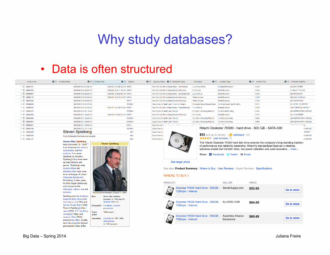
• Data is often structured – We can exploit this regular structure
• To retrieve data in useful ways (that is, we can use a query language)
• To store data efficiently

Big Data – Spring 2014 Juliana Freire
Why study databases?
• Data is often structured • We can exploit this regular structure
– To retrieve data in useful ways (that is, we can use a query language)
– To store data efficiently
Big Data – Spring 2014 Juliana Freire
Why study Databases? • Understand concepts and apply to different
problems and different areas, e.g., Big Data • Because DBMS software is highly successful as
a commercial technology (Oracle, DB2, MS SQL Server…)
• Because DB research is highly active and **very** interesting! – Lots of opportunities to have practical impact
Database Systems: The Basics
Big Data – Spring 2014 Juliana Freire
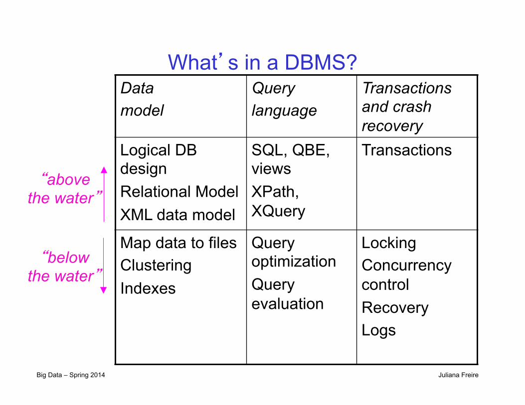
What’s in a DBMS?
“above the water”
“below the water”
Data model
Query language
Transactions and crash recovery
Logical DB design Relational Model XML data model
SQL, QBE, views XPath, XQuery
Transactions
Map data to files Clustering Indexes
Query optimization Query evaluation
Locking Concurrency control Recovery Logs
Big Data – Spring 2014 Juliana Freire
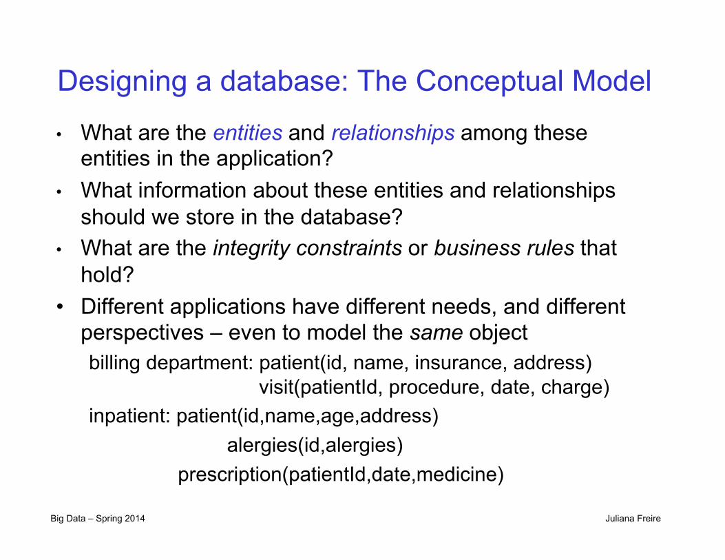
Designing a database: The Conceptual Model
• What are the entities and relationships among these entities in the application?
• What information about these entities and relationships should we store in the database?
• What are the integrity constraints or business rules that hold?
• Different applications have different needs, and different perspectives – even to model the same object billing department: patient(id, name, insurance, address)
visit(patientId, procedure, date, charge) inpatient: patient(id,name,age,address)
alergies(id,alergies) prescription(patientId,date,medicine)
Big Data – Spring 2014 Juliana Freire
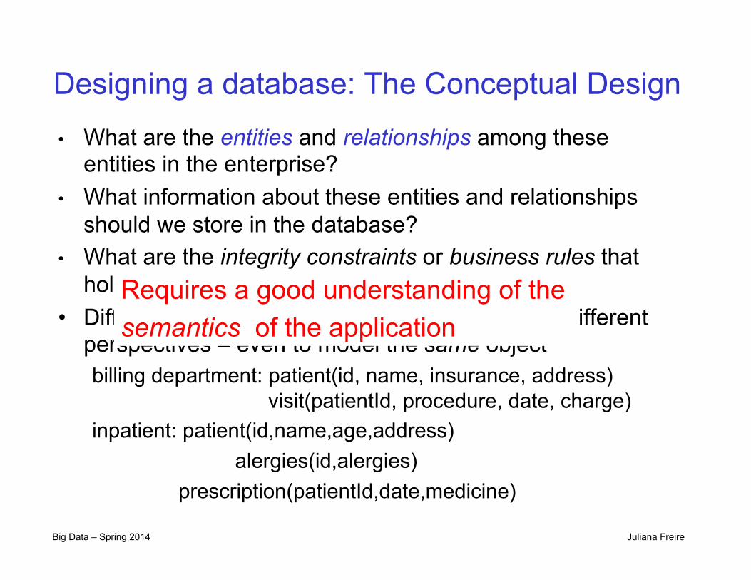
Designing a database: The Conceptual Design
• What are the entities and relationships among these entities in the enterprise?
• What information about these entities and relationships should we store in the database?
• What are the integrity constraints or business rules that hold?
• Different applications have different needs, and different perspectives – even to model the same object billing department: patient(id, name, insurance, address)
visit(patientId, procedure, date, charge) inpatient: patient(id,name,age,address)
alergies(id,alergies) prescription(patientId,date,medicine)
Requires a good understanding of the semantics of the application
Big Data – Spring 2014 Juliana Freire
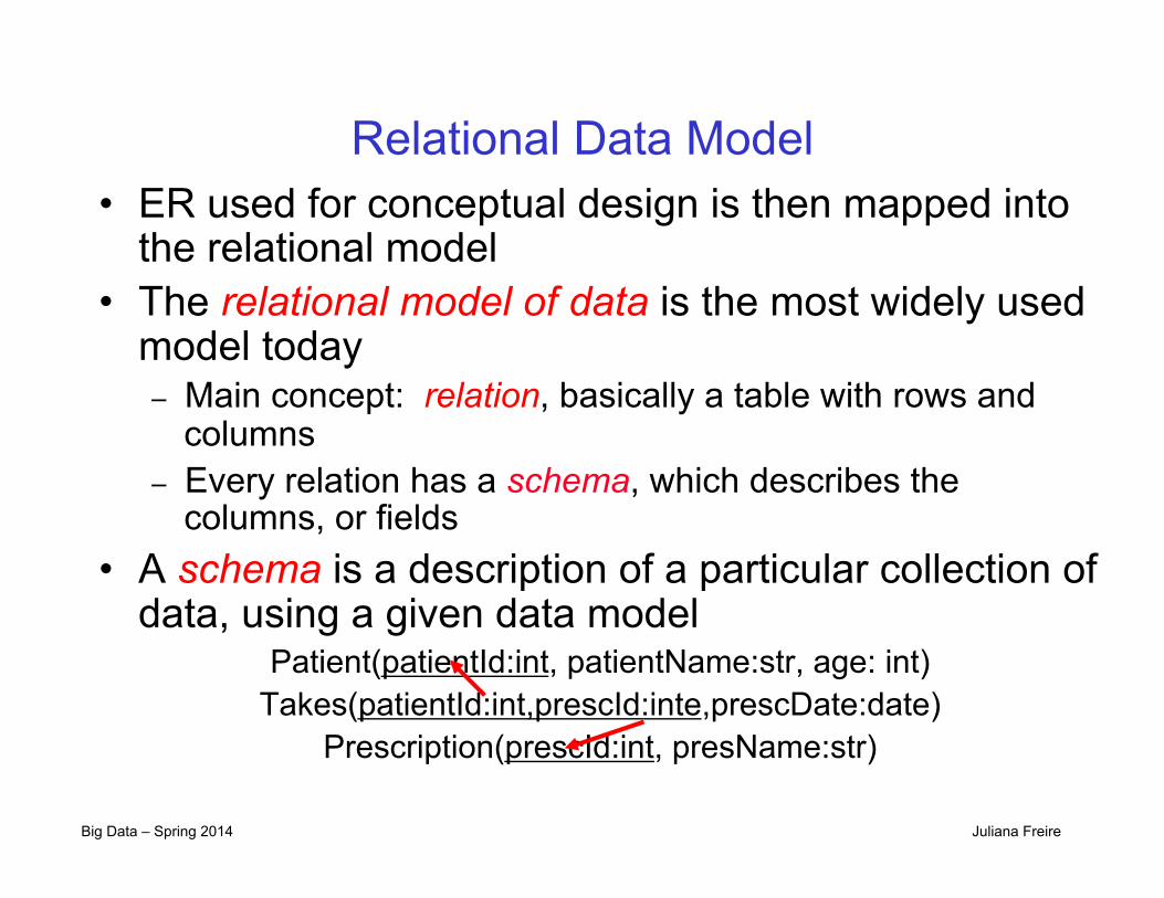
Relational Data Model • ER used for conceptual design is then mapped into
the relational model • The relational model of data is the most widely used
model today – Main concept: relation, basically a table with rows and
columns – Every relation has a schema, which describes the
columns, or fields • A schema is a description of a particular collection of
data, using a given data model Patient(patientId:int, patientName:str, age: int)
Takes(patientId:int,prescId:inte,prescDate:date) Prescription(prescId:int, presName:str)
Big Data – Spring 2014 Juliana Freire
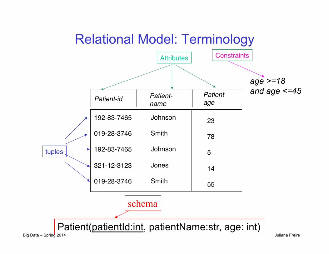
Relational Model: Terminology
Patient-!name!Patient-id" Patient-!
age!
Johnson""Smith""Johnson""Jones""Smith"
192-83-7465""019-28-3746""192-83-7465""321-12-3123""019-28-3746"
23""78""5""14""55"
Attributes"
tuples"
Patient(patientId:int, patientName:str, age: int)
schema
age >=18 and age <=45
Constraints"

Big Data – Spring 2014 Juliana Freire
Pitfalls in Relational Database Design • Find a “good” collection of relation schemas • Bad design may lead to
– Repetition of information à inconsistencies! • E.g., keeping people and addresses in a single file
– Inability to represent certain information • E.g., a doctor that is both a cardiologist and a pediatrician
• Design Goals: – Avoid redundant data – Ensure that relationships among attributes are
represented – Ensure constraints are properly modeled: updates
check for violation of database integrity constraints

Big Data – Spring 2014 Juliana Freire
Query Languages • Query languages: Allow manipulation and retrieval of data
from a database • Queries are posed wrt data model
– Operations over objects defined in data model • Relational model supports simple, powerful QLs:
– Strong formal foundation based on logic – Allows for optimization
• Query Languages != programming languages – QLs support easy, efficient access to large data sets – QLs not expected to be “Turing complete” – QLs not intended to be used for complex calculations

Big Data – Spring 2014 Juliana Freire
Query Languages
• Query languages: Allow manipulation and retrieval of data from a database.
• Relational model supports simple, powerful QLs: – Strong formal foundation based on logic. – Allows for much optimization.
• Query Languages != programming languages! – QLs not expected to be “Turing complete”. – QLs support easy, efficient access to large data sets. – QLs not intended to be used for complex calculations.
a language that can compute anything
that can be computed
Big Data – Spring 2014 Juliana Freire
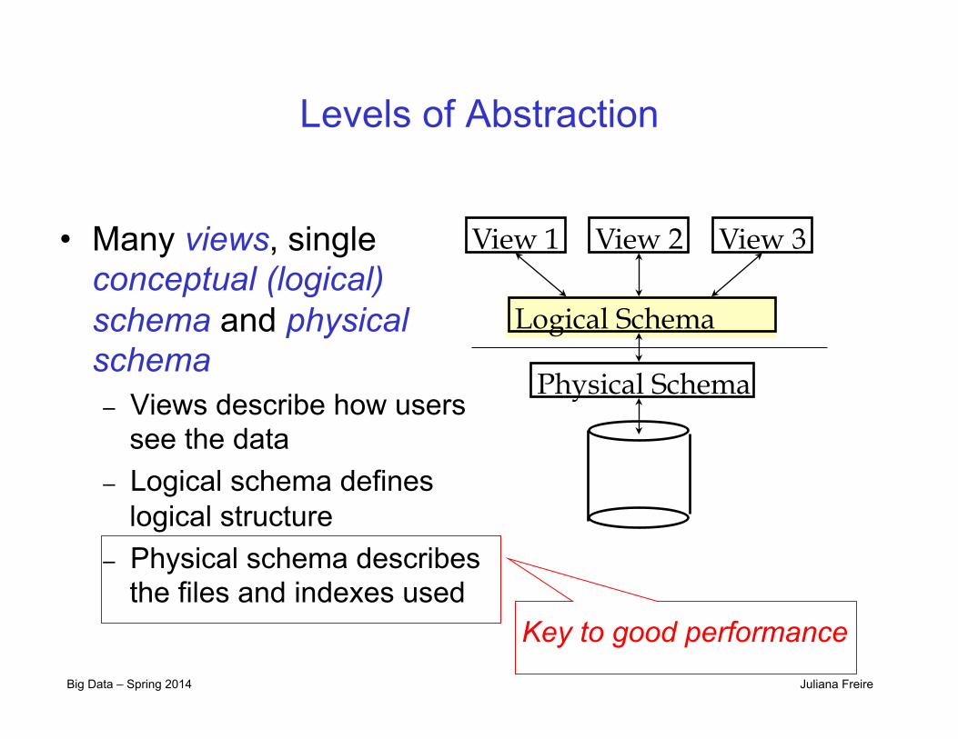
Levels of Abstraction
• Many views, single conceptual (logical) schema and physical schema – Views describe how users
see the data – Logical schema defines
logical structure – Physical schema describes
the files and indexes used
Physical Schema
Logical Schema
View 1 View 2 View 3
Key to good performance

Big Data – Spring 2014 Juliana Freire
Data Independence
• Applications insulated from how data is structured and stored
• Logical data independence: Protection from changes in logical structure of data – Changes in the logical schema do not affect users
as long as their views are still available • Physical data independence: Protection
from changes in physical structure of data – Changes in the physical layout of the data or in the
indexes used do not affect the logical relations
One of the most important benefits of using a DBMS!
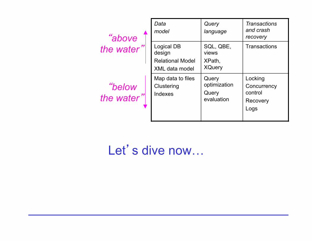
Let’s dive now…
“above the water”
“below the water”
Data model
Query language
Transactions and crash recovery
Logical DB design Relational Model XML data model
SQL, QBE, views XPath, XQuery
Transactions
Map data to files Clustering Indexes
Query optimization Query evaluation
Locking Concurrency control Recovery Logs

Big Data – Spring 2014 Juliana Freire
Storage and Indexing
• The DB administrator designs the physical structures • Nowadays, database systems can do (some of) this
automatically: autoadmin, index advisors • File structures: sequential, hashing, clustering, single
or multiple disks, etc. • Example – Bank accounts
– Good for: List all accounts in the Downtown branch – What about: List all accounts with balance = 350
Big Data – Spring 2014 Juliana Freire
Storage and Indexing
• Indexes: – Select attributes to index – Select the type of index
• Storage manager is a module that provides the interface between the low-level data stored in the database and the application programs and queries submitted to the system: – interaction with the file manager – efficient storing, retrieving and updating of data
Big Data – Spring 2014 Juliana Freire
Query Optimization and Evaluation
• DBMS must provide efficient access to data – In an emergency, can't wait 10 minutes to find
patient allergies • Declarative queries are translated into
imperative query plans – Declarative queries à logical data model – Imperative plans à physical structure
• Relational optimizers aim to find the best imperative plans (i.e., shortest execution time) – In practice they avoid the worst plans…
Big Data – Spring 2014 Juliana Freire
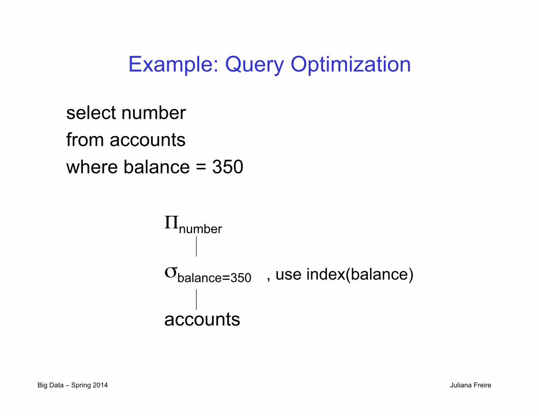
Example: Query Optimization
select number from accounts where balance = 350
Πnumber
σbalance=350
accounts
, use index(balance)
Big Data – Spring 2014 Juliana Freire
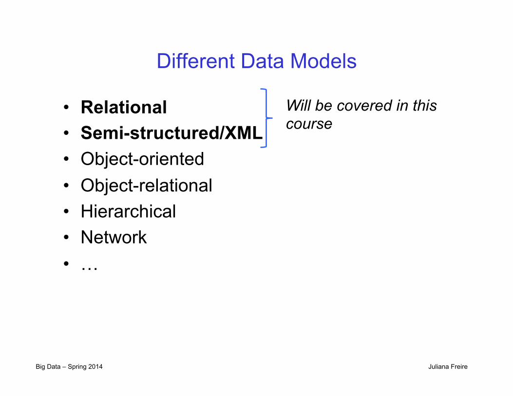
Different Data Models
• Relational • Semi-structured/XML • Object-oriented • Object-relational • Hierarchical • Network • …
Will be covered in this course
Big Data – Spring 2014 Juliana Freire
XML: A First Step Towards Convergence
• XML = Extensible Markup Language. • XML is syntactically related to HTML • Goal is different:
– HTML describes document structure – XML transmits textual data
• XML solves the data exchange problem – No need to write specialized wrappers. – The schema of an XML document serves as a contract
• XML does not solve the problem of efficient access – DB research is doing that! – Storage techniques, mechanisms for maintaining data
integrity and consistency,…
Big Data – Spring 2014 Juliana Freire
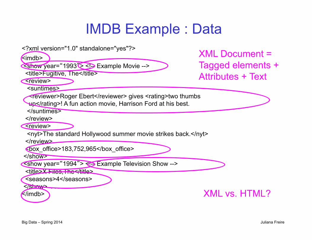
IMDB Example : Data <?xml version="1.0" standalone="yes"?> <imdb> <show year=“1993”> <!-- Example Movie --> <title>Fugitive, The</title> <review> <suntimes> <reviewer>Roger Ebert</reviewer> gives <rating>two thumbs up</rating>! A fun action movie, Harrison Ford at his best. </suntimes> </review> <review> <nyt>The standard Hollywood summer movie strikes back.</nyt> </review> <box_office>183,752,965</box_office> </show> <show year=“1994”> <!-- Example Television Show --> <title>X Files,The</title> <seasons>4</seasons> </show> . . . </imdb>
XML Document = Tagged elements + Attributes + Text
XML vs. HTML?
Big Data – Spring 2014 Juliana Freire
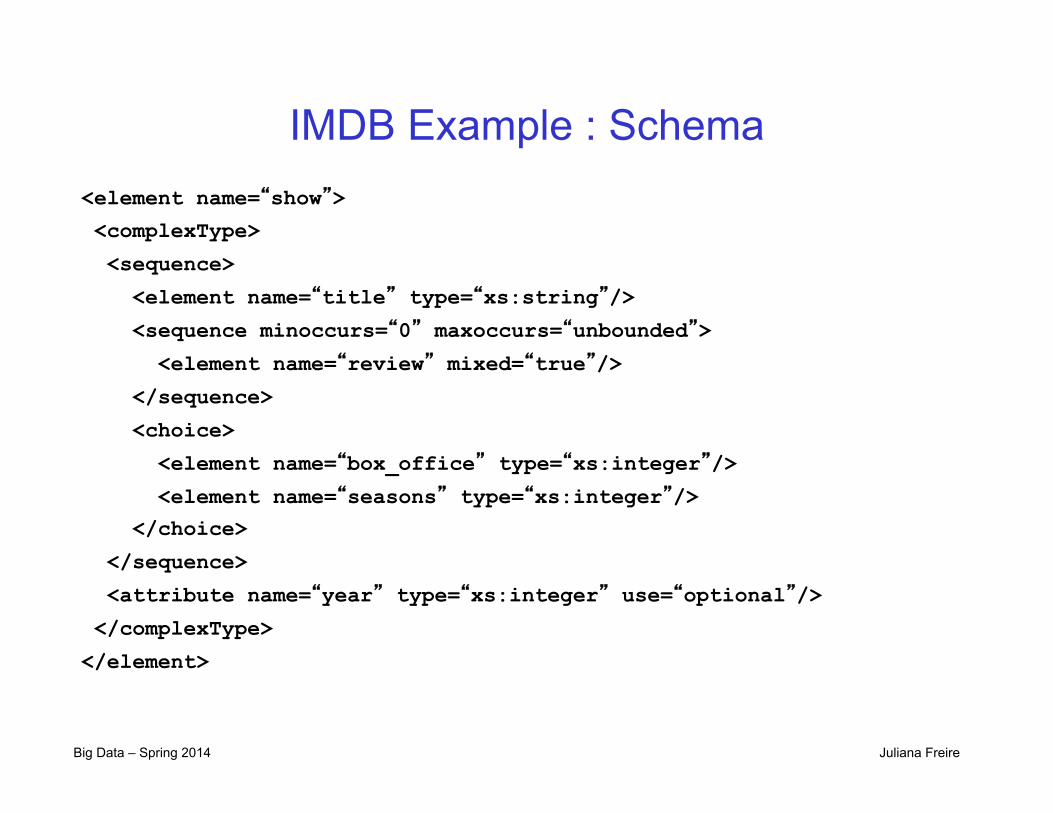
IMDB Example : Schema <element name=“show”>
<complexType>
<sequence>
<element name=“title” type=“xs:string”/>
<sequence minoccurs=“0” maxoccurs=“unbounded”>
<element name=“review” mixed=“true”/>
</sequence>
<choice>
<element name=“box_office” type=“xs:integer”/>
<element name=“seasons” type=“xs:integer”/>
</choice>
</sequence>
<attribute name=“year” type=“xs:integer” use=“optional”/>
</complexType>
</element>
Big Data – Spring 2014 Juliana Freire
Key Concepts in Databases
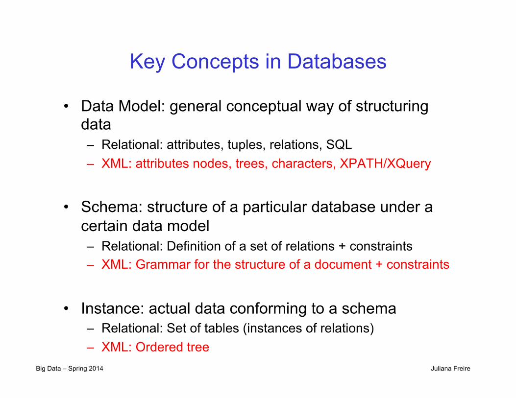
• Data Model: general conceptual way of structuring data – Relational: attributes, tuples, relations, SQL – XML: attributes nodes, trees, characters, XPATH/XQuery
• Schema: structure of a particular database under a certain data model – Relational: Definition of a set of relations + constraints – XML: Grammar for the structure of a document + constraints
• Instance: actual data conforming to a schema
– Relational: Set of tables (instances of relations) – XML: Ordered tree
Big Data – Spring 2014 Juliana Freire
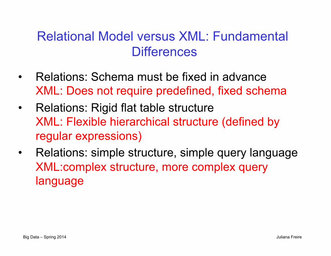
Relational Model versus XML: Fundamental Differences
• Relations: Schema must be fixed in advance XML: Does not require predefined, fixed schema
• Relations: Rigid flat table structure XML: Flexible hierarchical structure (defined by regular expressions)
• Relations: simple structure, simple query language XML:complex structure, more complex query language
Big Data – Spring 2014 Juliana Freire
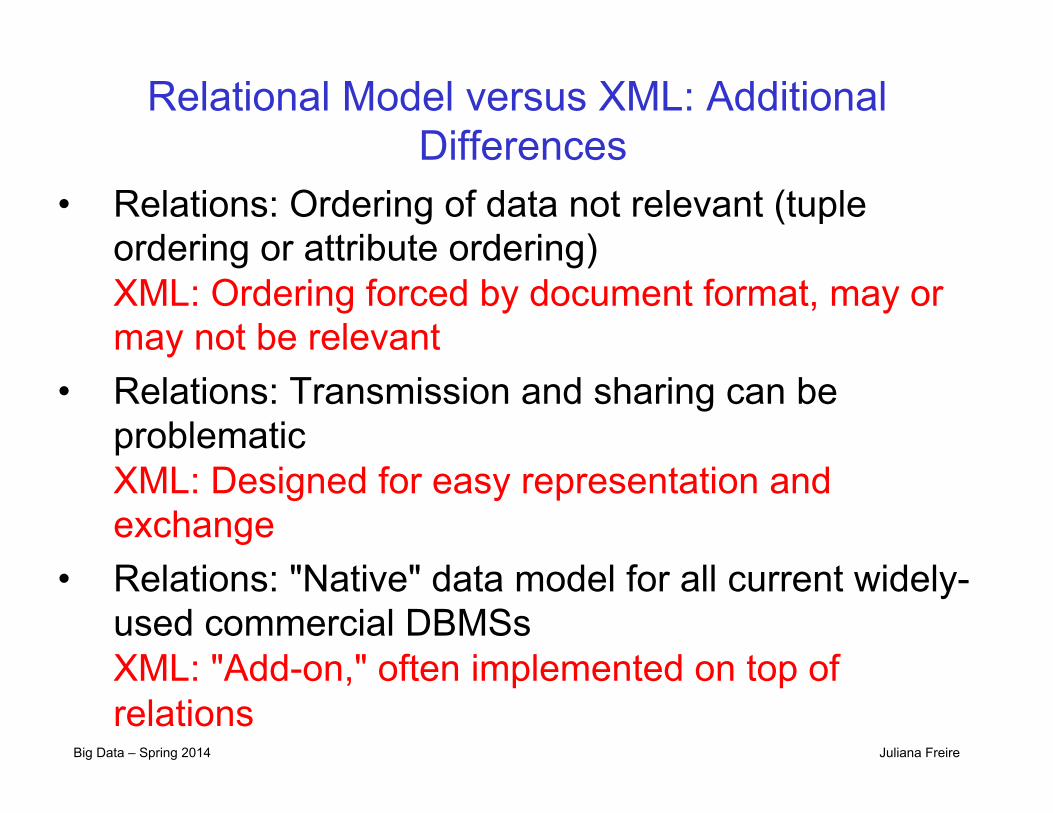
Relational Model versus XML: Additional Differences
• Relations: Ordering of data not relevant (tuple ordering or attribute ordering) XML: Ordering forced by document format, may or may not be relevant
• Relations: Transmission and sharing can be problematic XML: Designed for easy representation and exchange
• Relations: "Native" data model for all current widely-used commercial DBMSs XML: "Add-on," often implemented on top of relations

Big Data – Spring 2014 Juliana Freire
Formal Relational Query Languages
• Two mathematical Query Languages form the basis for “real” relational languages (e.g., SQL), and for implementation: – Relational Algebra: More operational, very useful
for representing execution plans. – Relational Calculus: Lets users describe what
they want, rather than how to compute it. (Non-operational, declarative.)
Big Data – Spring 2014 Juliana Freire
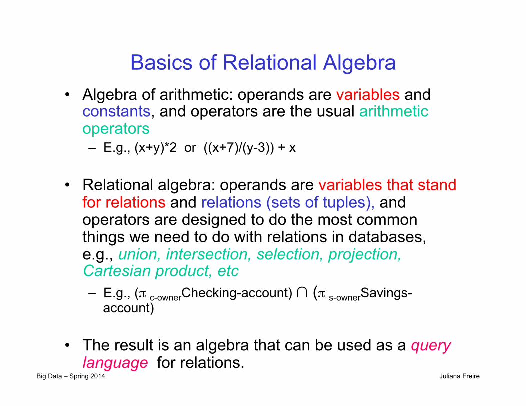
Basics of Relational Algebra • Algebra of arithmetic: operands are variables and
constants, and operators are the usual arithmetic operators – E.g., (x+y)*2 or ((x+7)/(y-3)) + x
• Relational algebra: operands are variables that stand for relations and relations (sets of tuples), and operators are designed to do the most common things we need to do with relations in databases, e.g., union, intersection, selection, projection, Cartesian product, etc – E.g., (π c-ownerChecking-account) ∩ (π s-ownerSavings-
account)
• The result is an algebra that can be used as a query language for relations.

Big Data – Spring 2014 Juliana Freire
Why SQL?
• SQL is a high-level language – Say “what to do” rather than “how to do it” – Avoid a lot of data-manipulation details needed in
procedural languages like C++ or Java • Database management system figures out “best” way to execute query – Called “query optimization”
Big Data – Spring 2014 Juliana Freire
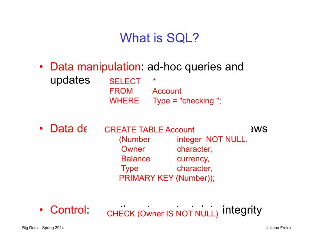
What is SQL?
• Data manipulation: ad-hoc queries and updates
• Data definition: creation of tables and views
• Control: assertions to protect data integrity
SELECT * FROM Account WHERE Type = "checking ";
CREATE TABLE Account (Number integer NOT NULL, Owner character,
Balance currency, Type character, PRIMARY KEY (Number));
CHECK (Owner IS NOT NULL)
Big Data – Spring 2014 Juliana Freire
Relational Algebra vs. SQL
• Relational algebra = query only • SQL = data manipulation + data definition +
control • SQL data manipulation is similar to, but not
exactly the same as relational algebra – SQL is based on set and relational operations with
certain modifications and enhancements – We will study the differences
• We coverage the various operations and some details about using SQL

Big Data – Spring 2014 Juliana Freire
MapReduce • Large data • New parallel architectures
“Work”
w1 w2 w3
r1 r2 r3
“Result”
“worker” “worker” “worker”
Partition
Combine
Big Data – Spring 2014 Juliana Freire
Parallelization Challenges
• How do we assign work units to workers? • What if we have more work units than
workers? • What if workers need to share partial results? • How do we aggregate partial results? • How do we know all the workers have
finished? • What if workers die? What is the common theme of all of these problems?

Big Data – Spring 2014 Juliana Freire
Common Theme?
• Parallelization problems arise from: – Communication between workers (e.g., to
exchange state) – Access to shared resources (e.g., data)
• Thus, we need a synchronization mechanism
Big Data – Spring 2014 Juliana Freire
Managing Multiple Workers
• Difficult because – We don’t know the order in which workers run – We don’t know when workers interrupt each other – We don’t know the order in which workers access shared data
• Thus, we need: – Semaphores (lock, unlock) – Conditional variables (wait, notify, broadcast) – Barriers
• Still, lots of problems: – Deadlock, livelock, race conditions... – Dining philosophers, sleeping barbers, cigarette smokers...
• Moral of the story: be careful!

Big Data – Spring 2014 Juliana Freire
Current Tools
• Programming models – Shared memory (pthreads) – Message passing (MPI)
• Design Patterns – Master-slaves – Producer-consumer flows – Shared work queues
Message Passing
P1 P2 P3 P4 P5
Shared Memory
P1 P2 P3 P4 P5
Mem
ory
master
slaves
producer consumer
producer consumer
work queue
Big Data – Spring 2014 Juliana Freire
Where the rubber meets the road
• Concurrency is difficult to reason about • Concurrency is even more difficult to reason about
– At the scale of datacenters (even across datacenters) – In the presence of failures – In terms of multiple interacting services
• Not to mention debugging… • The reality:
– Lots of one-off solutions, custom code – Write you own dedicated library, then program with it – Burden on the programmer to explicitly manage everything
Big Data – Spring 2014 Juliana Freire
What’s the point?
• It’s all about the right level of abstraction – The von Neumann architecture has served us well,
but is no longer appropriate for the multi-core/cluster environment
• Hide system-level details from the developers – No more race conditions, lock contention, etc.
• Separating the what from how – Developer specifies the computation that needs to
be performed – Execution framework (“runtime”) handles actual
execution
The datacenter is the computer!
Big Data – Spring 2014 Juliana Freire
Big Ideas: Scale Out vs. Scale Up • Scale up: small number of high-end servers
– Symmetric multi-processing (SMP) machines, large shared memory
l Not cost-effective – cost of machines does not scale linearly; and no single SMP machine is big enough
• Scale out: Large number of commodity low-end servers is more effective for data-intensive applications – 8 128-core machines vs. 128 8-core machines
“low-end server platform is about 4 times more cost efficient than a high-end shared memory platform from the same vendor”, Barroso and Hölzle, 2009
Big Data – Spring 2014 Juliana Freire
Big Ideas: Failures are Common
• Suppose a cluster is built using machines with a mean-time between failures (MTBF) of 1000 days
• For a 10,000 server cluster, there are on average 10 failures per day!
• MapReduce implementation cope with failures – Automatic task restarts
Big Data – Spring 2014 Juliana Freire
Big Ideas: Move Processing to Data
• Supercomputers often have processing nodes and storage nodes – Computationally expensive tasks – High-capacity interconnect to move data around
• Many data-intensive applications are not very processor-demanding – Data movement leads to a bottleneck in the network! – New idea: move processing to where the data reside
• In MapReduce, processors and storage are co-located – Leverage locality

Big Data – Spring 2014 Juliana Freire
Big Ideas: Avoid Random Access • Disk seek times are determined by mechanical
factors – Read heads can only move so fast and platters can
only spin so rapidly
Big Data – Spring 2014 Juliana Freire
Big Ideas: Avoid Random Access Example:
– 1 TB database containing 1010 100 byte records – Random access: each update takes ~30ms
(seek ,read, write) • Updating 1% of the records takes ~35 days
– Sequential access: 100MB/s throughput • Reading the whole database and rewriting all the records,
takes 5.6 hours
• MapReduce was designed for batch processing --- organize computations into long streaming operations
Big Data – Spring 2014 Juliana Freire
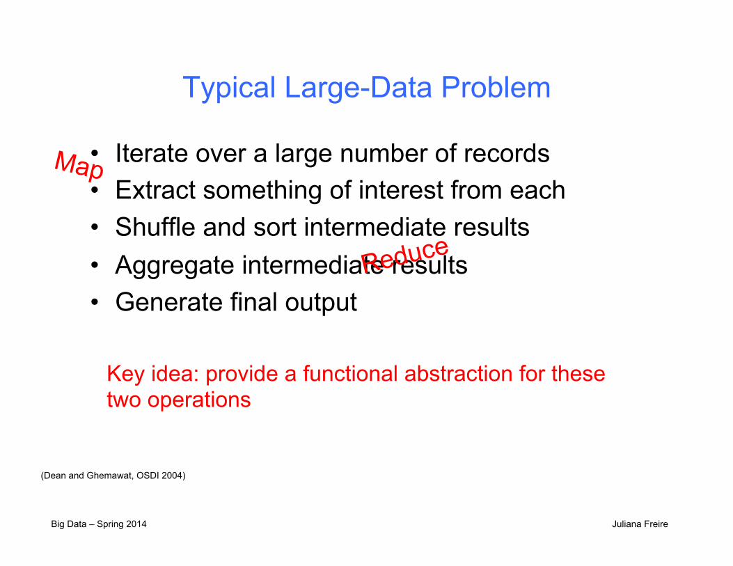
Typical Large-Data Problem
• Iterate over a large number of records • Extract something of interest from each • Shuffle and sort intermediate results • Aggregate intermediate results • Generate final output
Key idea: provide a functional abstraction for these two operations
Map
Reduce
(Dean and Ghemawat, OSDI 2004)
Big Data – Spring 2014 Juliana Freire
Map and Reduce
• The idea of Map, and Reduce is 40+ year old - Present in all Functional Programming Languages. - See, e.g., APL, Lisp and ML
• Alternate names for Map: Apply-All • Higher Order Functions - take function definitions as arguments, or - return a function as output
• Map and Reduce are higher-order functions.
Big Data – Spring 2014 Juliana Freire
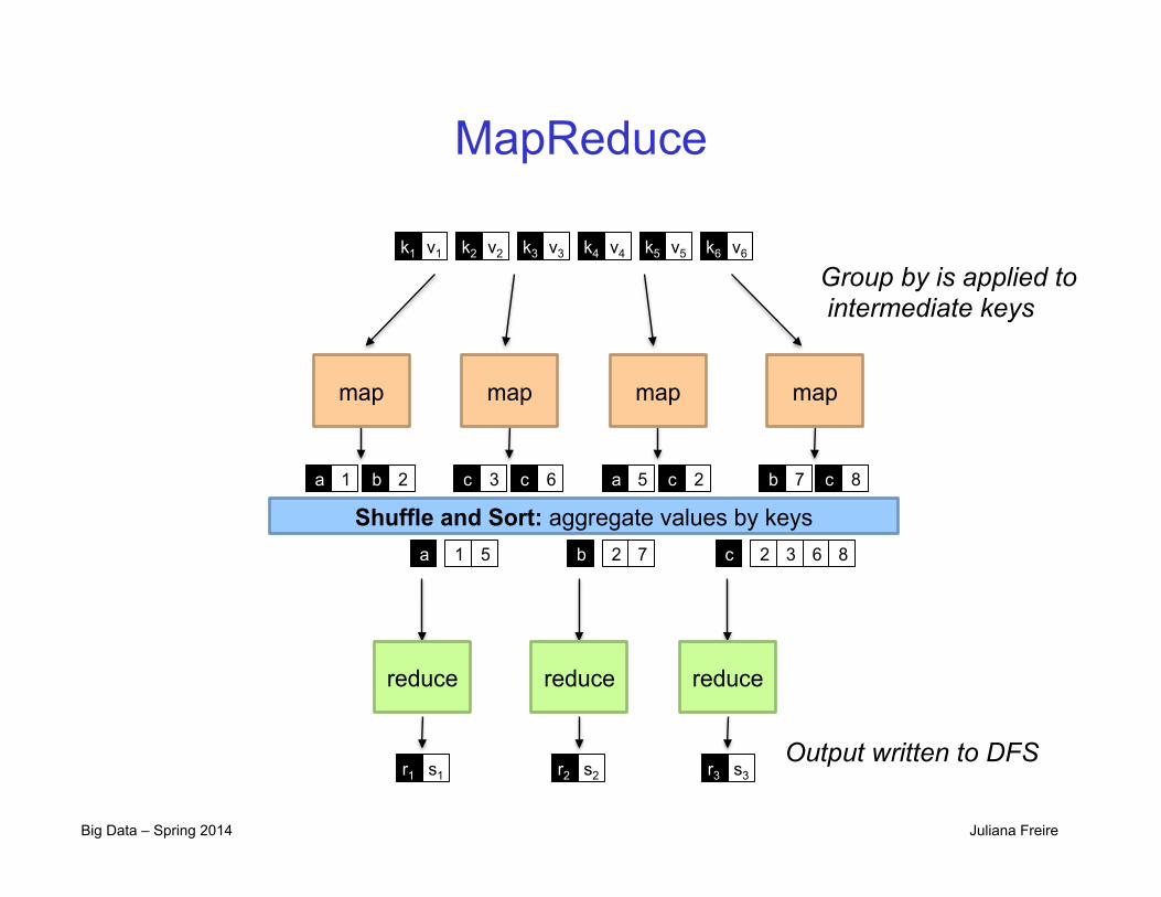
MapReduce
Big Data – Spring 2014 Juliana Freire
map map map map
Shuffle and Sort: aggregate values by keys
reduce reduce reduce
k1 k2 k3 k4 k5 k6 v1 v2 v3 v4 v5 v6
b a 1 2 c c 3 6 a c 5 2 b c 7 8
a 1 5 b 2 7 c 2 3 6 8
r1 s1 r2 s2 r3 s3
Group by is applied to intermediate keys
Output written to DFS

Big Data – Spring 2014 Juliana Freire
Two more details…
• Barrier between map and reduce phases – But we can begin copying intermediate data earlier
• Keys arrive at each reducer in sorted order – No enforced ordering across reducers

Big Data – Spring 2014 Juliana Freire
MapReduce “Runtime”
• Handles scheduling – Assigns workers to map and reduce tasks
• Handles “data distribution” – Moves processes to data
• Handles synchronization – Gathers, sorts, and shuffles intermediate data
• Handles errors and faults – Detects worker failures and restarts
• Everything happens on top of a distributed FS (later)

Big Data – Spring 2014 Juliana Freire
MapReduce: The Complete Picture
Big Data – Spring 2014 Juliana Freire
combine combine combine combine
b a 1 2 c 9 a c 5 2 b c 7 8
partition partition partition partition
map map map map
k1 k2 k3 k4 k5 k6 v1 v2 v3 v4 v5 v6
b a 1 2 c c 3 6 a c 5 2 b c 7 8
Shuffle and Sort: aggregate values by keys
reduce reduce reduce
a 1 5 b 2 7 c 2 9 8
r1 s1 r2 s2 r3 s3
c 2 3 6 8
Big Data – Spring 2014 Juliana Freire
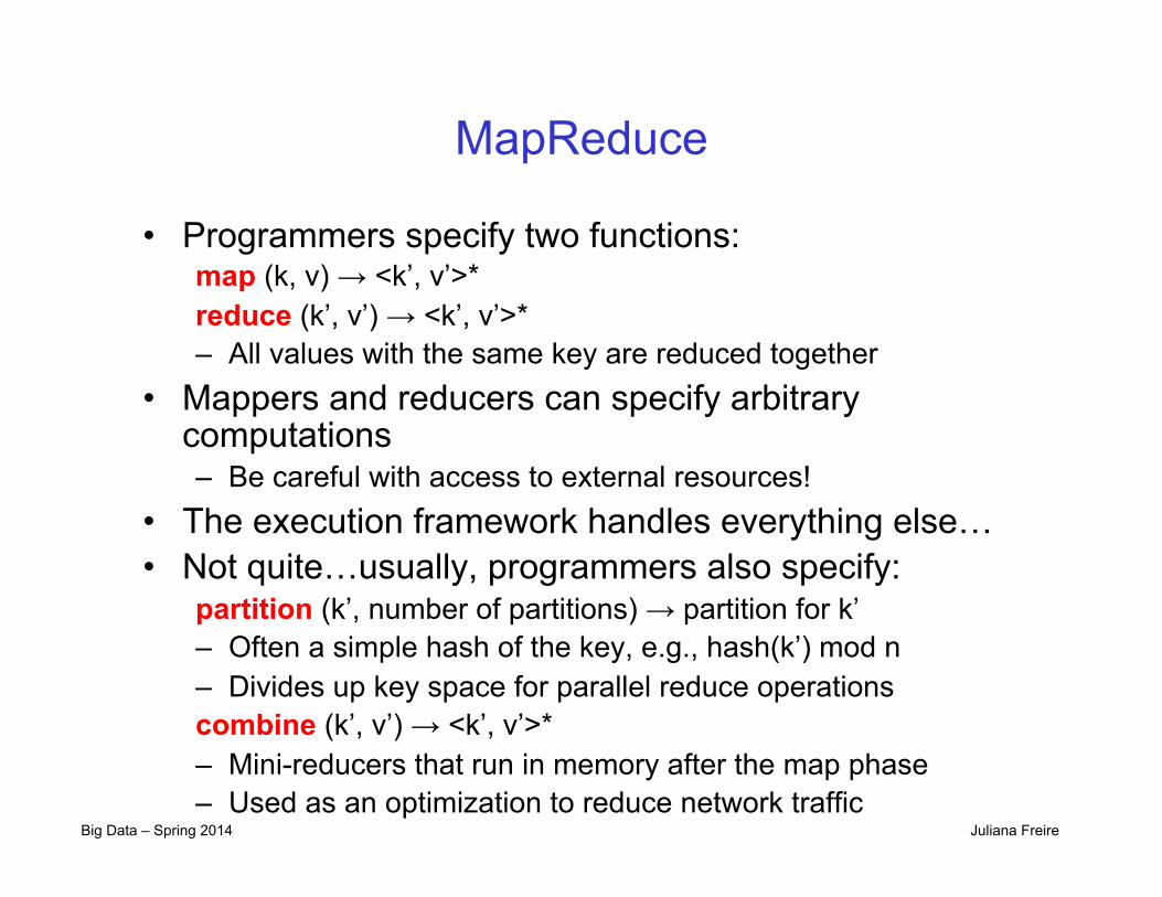
MapReduce
• Programmers specify two functions: map (k, v) → <k’, v’>* reduce (k’, v’) → <k’, v’>* – All values with the same key are reduced together
• Mappers and reducers can specify arbitrary computations – Be careful with access to external resources!
• The execution framework handles everything else… • Not quite…usually, programmers also specify:
partition (k’, number of partitions) → partition for k’ – Often a simple hash of the key, e.g., hash(k’) mod n – Divides up key space for parallel reduce operations combine (k’, v’) → <k’, v’>* – Mini-reducers that run in memory after the map phase – Used as an optimization to reduce network traffic
Big Data – Spring 2014 Juliana Freire
Distributed File System
• Don’t move data to workers… move workers to the data! – Store data on the local disks of nodes in the cluster – Start up the workers on the node that has the data
local • Why?
– Not enough RAM to hold all the data in memory – Disk access is slow, but disk throughput is
reasonable • A distributed file system is the answer
– GFS (Google File System) for Google’s MapReduce – HDFS (Hadoop Distributed File System) for Hadoop

Big Data – Spring 2014 Juliana Freire
GFS: Design Decisions
• Files stored as chunks – Fixed size (e.g., 64MB)
• Reliability through replication – Each chunk replicated across 3+ chunkservers
• Single master to coordinate access, keep metadata – Simple centralized management
• No data caching – Little benefit due to large datasets, streaming reads
• Simplify the API – Push some of the issues onto the client (e.g., data layout)
HDFS = GFS clone (same basic ideas)
Big Data – Spring 2014 Juliana Freire
Designing Algorithms for MapReduce • Need to adapt to a restricted model of
computation • Goals
– Scalability: adding machines will make the algo run faster
– Efficiency: resources will not be wasted
• The translation some algorithms into MapReduce isn’t always obvious
• But there are useful design patterns that can help
• We covered patterns and examples to illustrate how they can be applied
Big Data – Spring 2014 Juliana Freire
Tools for Synchronization
• Cleverly-constructed data structures – Bring partial results together
• Sort order of intermediate keys – Control order in which reducers process keys
• Partitioner – Control which reducer processes which keys
• Preserving state in mappers and reducers – Capture dependencies across multiple keys and
values

Big Data – Spring 2014 Juliana Freire
Strategy: Local Aggregation • Use combiners • Do aggregation inside mappers • In-mapper combining
– Fold the functionality of the combiner into the mapper by preserving state across multiple map calls
• Advantages – Explicit control aggregation – Speed
• Disadvantages – Explicit memory management required – Potential for order-dependent bugs
Big Data – Spring 2014 Juliana Freire
Limiting Memory Usage • To limit memory usage when using the in-mapper
combining technique, block input key-value pairs and flush in-memory data structures periodically – E.g., counter variable that keeps track of the number of input key-
value pairs that have been processed
• Memory usage threshold needs to be determined empirically: with too large a value, the mapper may run out of memory, but with too small a value, opportunities for local aggregation may be lost
• Note: Hadoop physical memory is split between multiple tasks that may be running on a node concurrently – difficult to coordinate resource consumption
Big Data – Spring 2014 Juliana Freire
Combiner Design
• Combiners and reducers share same method signature – Sometimes, reducers can serve as combiners
When is this the case? – Often, not…works only when reducer is
commutative and associative • Remember: combiner are optional
optimizations – Should not affect algorithm correctness – May be run 0, 1, or multiple times
• Example: find average of all integers associated with the same key
Big Data – Spring 2014 Juliana Freire
MapReduce: Large Counting Problems • Term co-occurrence matrix for a text collection
= specific instance of a large counting problem – A large event space (number of terms) – A large number of observations (the collection itself) – Goal: keep track of interesting statistics about the events
• Basic approach – Mappers generate partial counts – Reducers aggregate partial counts
How do we aggregate partial counts efficiently?
Big Data – Spring 2014 Juliana Freire
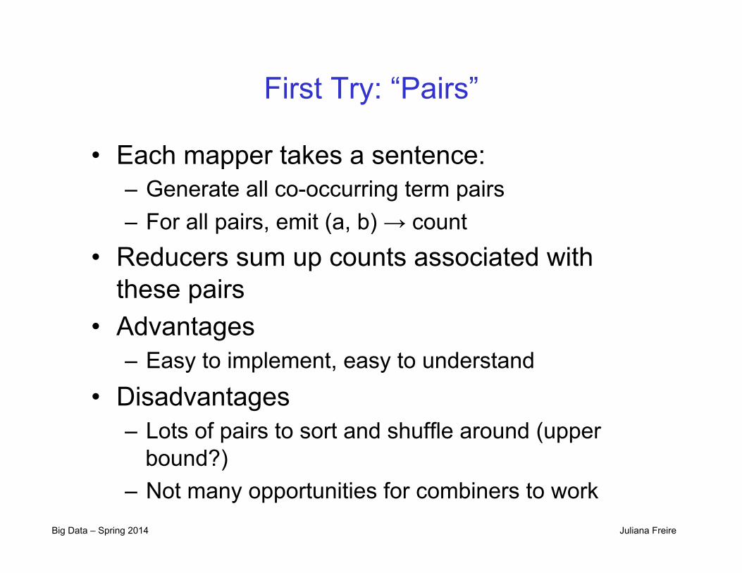
First Try: “Pairs”
• Each mapper takes a sentence: – Generate all co-occurring term pairs – For all pairs, emit (a, b) → count
• Reducers sum up counts associated with these pairs
• Advantages – Easy to implement, easy to understand
• Disadvantages – Lots of pairs to sort and shuffle around (upper
bound?) – Not many opportunities for combiners to work
Big Data – Spring 2014 Juliana Freire
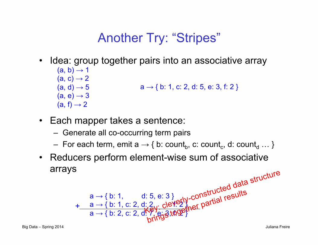
Another Try: “Stripes”
• Idea: group together pairs into an associative array
• Each mapper takes a sentence: – Generate all co-occurring term pairs – For each term, emit a → { b: countb, c: countc, d: countd … }
• Reducers perform element-wise sum of associative arrays
(a, b) → 1 (a, c) → 2 (a, d) → 5 (a, e) → 3 (a, f) → 2
a → { b: 1, c: 2, d: 5, e: 3, f: 2 }
a → { b: 1, d: 5, e: 3 } a → { b: 1, c: 2, d: 2, f: 2 } a → { b: 2, c: 2, d: 7, e: 3, f: 2 }
+ Key: cleverly-constructed data structure
brings together partial results

Big Data – Spring 2014 Juliana Freire
“Stripes” Analysis
• Advantages – Far less sorting and shuffling of key-value pairs – Can make better use of combiners
• Disadvantages – More difficult to implement – Underlying object more heavyweight – Fundamental limitation in terms of size of event
space
Big Data – Spring 2014 Juliana Freire
“Order Inversion”
• Common design pattern – Computing relative frequencies requires marginal
counts – But marginal cannot be computed until you see all
counts – Buffering is a bad idea! – Trick: getting the marginal counts to arrive at the
reducer before the joint counts • Optimizations
– Apply in-memory combining pattern to accumulate marginal counts
– Should we apply combiners?

Big Data – Spring 2014 Juliana Freire
The Debate Starts…
Big Data – Spring 2014 Juliana Freire
The Debate Continues…
• A comparison of approaches to large-scale data analysis. Pavlo et al., SIGMOD 2009 – Parallel DBMS beats MapReduce by a lot! – Many were outraged by the comparison
• MapReduce: A Flexible Data Processing Tool. Dean and Ghemawat, CACM 2010 – Pointed out inconsistencies and mistakes in the
comparison • MapReduce and Parallel DBMSs: Friends or
Foes? Stonebraker et al., CACM 2010 – Toned down claims…
Big Data – Spring 2014 Juliana Freire
Parallel DBMSs
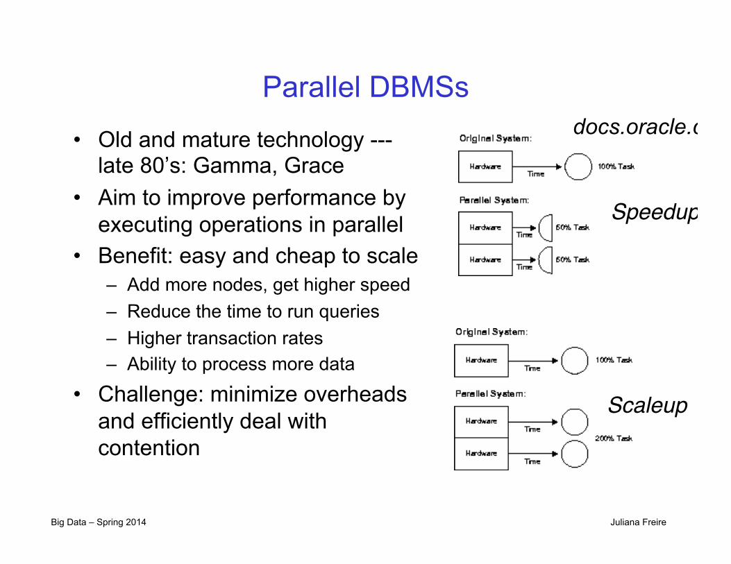
• Old and mature technology --- late 80’s: Gamma, Grace
• Aim to improve performance by executing operations in parallel
• Benefit: easy and cheap to scale – Add more nodes, get higher speed – Reduce the time to run queries – Higher transaction rates – Ability to process more data
• Challenge: minimize overheads and efficiently deal with contention
docs.oracle.com
Speedup!
Scaleup!
Big Data – Spring 2014 Juliana Freire
Partitioning a Relation across Disks
• If a relation contains only a few tuples which will fit into a single disk block, then assign the relation to a single disk
• Large relations are preferably partitioned across all the available disks
• The distribution of tuples to disks may be skewed — that is, some disks have many tuples, while others may have fewer tuples
• Ideal: partitioning should be balanced
Big Data – Spring 2014 Juliana Freire
Horizontal Data Partitioning
• Relation R split into P chunks R0, ..., RP-1, stored at the P nodes
• Round robin: tuple Ti to chunk (i mod P) • Hash based partitioning on attribute A:
– Tuple t to chunk h(t.A) mod P
• Range based partitioning on attribute A: – Tuple t to chunk i if vi-1 <t.A<vi – E.g., with a partitioning vector [5,11], a tuple with partitioning
attribute value of 2 will go to disk 0, a tuple with value 8 will go to disk 1, while a tuple with value 20 will go to disk 2.
Partitioning in Oracle: http://docs.oracle.com/cd/B10501_01/server.920/a96524/c12parti.htm Partitioning in DB2: http://www.ibm.com/developerworks/data/library/techarticle/dm-0605ahuja2/
Big Data – Spring 2014 Juliana Freire
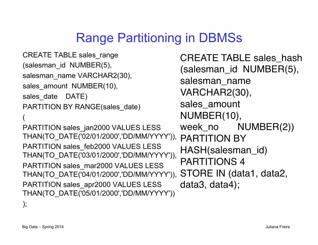
Range Partitioning in DBMSs CREATE TABLE sales_range (salesman_id NUMBER(5), salesman_name VARCHAR2(30), sales_amount NUMBER(10), sales_date DATE) PARTITION BY RANGE(sales_date) ( PARTITION sales_jan2000 VALUES LESS THAN(TO_DATE('02/01/2000','DD/MM/YYYY')), PARTITION sales_feb2000 VALUES LESS THAN(TO_DATE('03/01/2000','DD/MM/YYYY')), PARTITION sales_mar2000 VALUES LESS THAN(TO_DATE('04/01/2000','DD/MM/YYYY')), PARTITION sales_apr2000 VALUES LESS THAN(TO_DATE('05/01/2000','DD/MM/YYYY')) );
CREATE TABLE sales_hash"(salesman_id NUMBER(5), "salesman_name VARCHAR2(30), "sales_amount NUMBER(10), "week_no NUMBER(2)) "PARTITION BY HASH(salesman_id) "PARTITIONS 4 "STORE IN (data1, data2, data3, data4);"
Big Data – Spring 2014 Juliana Freire
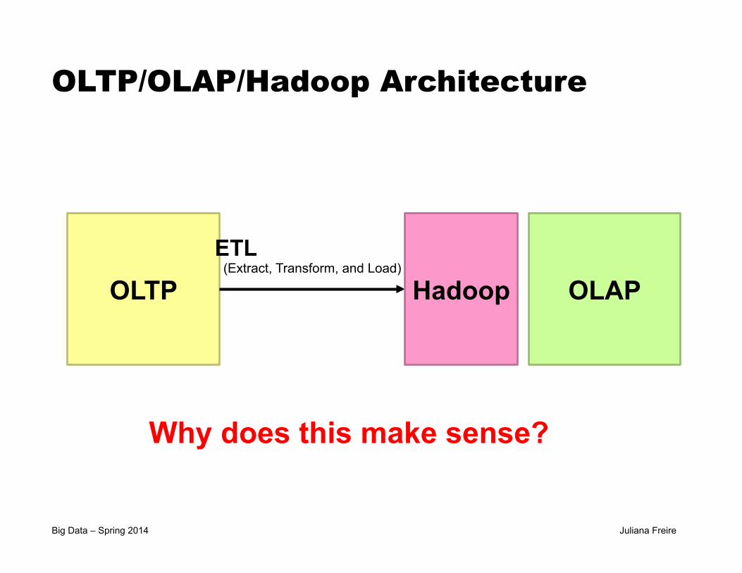
OLTP/OLAP/Hadoop Architecture
OLTP OLAP
ETL (Extract, Transform, and Load)
Hadoop
Why does this make sense?

Big Data – Spring 2014 Juliana Freire
Projection in MapReduce
• Easy • Map over tuples, emit new tuples with appropriate attributes • No reducers, unless for regrouping or resorting tuples • Alternatively: perform in reducer, after some other processing
• Basically limited by HDFS streaming speeds • Speed of encoding/decoding tuples becomes important • Semistructured data? No problem!
• And other relational operations…

Big Data – Spring 2014 Juliana Freire
Join Algorithms in MapReduce
• Reduce-side join • Map-side join • In-memory join
Big Data – Spring 2014 Juliana Freire
Reduce-Side Join
• Basic idea: group by join key – Map over both sets of tuples – Emit tuple as value with join key as the
intermediate key – Execution framework brings together tuples
sharing the same key – Perform actual join in reducer – Similar to a “sort-merge join” in database
terminology • Two variants
– 1-to-1 joins – 1-to-many and many-to-many joins
Big Data – Spring 2014 Juliana Freire
Map-Side Join: Parallel Scans
• If datasets are sorted by join key, join can be accomplished by a scan over both datasets
• How can we accomplish this in parallel? – Partition and sort both datasets in the same manner
• In MapReduce: – Map over one dataset, read from other corresponding
partition – No reducers necessary (unless to repartition or resort)
• Consistently partitioned datasets: realistic to expect? – Depends on the workflow – For ad hoc data analysis, reduce-side are more general,
although less efficient

Big Data – Spring 2014 Juliana Freire
In-Memory Join
• Basic idea: load one dataset into memory, stream over other dataset – Works if R << S and R fits into memory – Called a “hash join” in database terminology
• MapReduce implementation – Distribute R to all nodes – Map over S, each mapper loads R in memory,
hashed by join key – For every tuple in S, look up join key in R – No reducers, unless for regrouping or resorting
tuples

Big Data – Spring 2014 Juliana Freire
Need for High-Level Languages
• Hadoop is great for large-data processing! – But writing Java programs for everything is
verbose and slow – Not everyone wants to (or can) write Java code
• Solution: develop higher-level data processing languages – Hive: HQL is like SQL – Pig: Pig Latin is a bit like Perl
Big Data – Spring 2014 Juliana Freire
Hive and Pig
• Hive: data warehousing application in Hadoop – Query language is HQL, variant of SQL – Tables stored on HDFS as flat files – Developed by Facebook, now open source
• Pig: large-scale data processing system – Scripts are written in Pig Latin, a dataflow language – Developed by Yahoo!, now open source – Roughly 1/3 of all Yahoo! internal jobs
• Common idea: – Provide higher-level language to facilitate large-data
processing – Higher-level language “compiles down” to Hadoop jobs
Big Data – Spring 2014 Juliana Freire
Association Rule Discovery
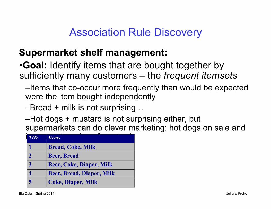
Supermarket shelf management: • Goal: Identify items that are bought together by sufficiently many customers – the frequent itemsets
– Items that co-occur more frequently than would be expected were the item bought independently – Bread + milk is not surprising… – Hot dogs + mustard is not surprising either, but supermarkets can do clever marketing: hot dogs on sale and increase the price of mustard
Supermarket shelf management – Market-basket model: � Goal: Identify items that are bought together by
sufficiently many customers � Approach: Process the sales data collected with barcode
scanners to find dependencies among items � A classic rule: � If one buys diaper and milk, then he is likely to buy beer � Don’t be surprised if you find six-packs next to diapers!
1/10/2013 Jure Leskovec, Stanford CS246: Mining Massive Datasets, http://cs246.stanford.edu 2
TID Items
1 Bread, Coke, Milk2 Beer, Bread3 Beer, Coke, Diaper, Milk4 Beer, Bread, Diaper, Milk5 Coke, Diaper, Milk
Rules Discovered: {Milk} --> {Coke} {Diaper, Milk} --> {Beer}
Big Data – Spring 2014 Juliana Freire
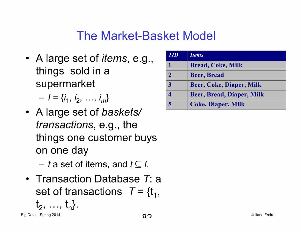
The Market-Basket Model
• A large set of items, e.g., things sold in a supermarket – I = {i1, i2, …, im}
• A large set of baskets/transactions, e.g., the things one customer buys on one day – t a set of items, and t ⊆ I.
• Transaction Database T: a set of transactions T = {t1, t2, …, tn}.
82
Supermarket shelf management – Market-basket model: � Goal: Identify items that are bought together by
sufficiently many customers � Approach: Process the sales data collected with barcode
scanners to find dependencies among items � A classic rule: � If one buys diaper and milk, then he is likely to buy beer � Don’t be surprised if you find six-packs next to diapers!
1/10/2013 Jure Leskovec, Stanford CS246: Mining Massive Datasets, http://cs246.stanford.edu 2
TID Items
1 Bread, Coke, Milk2 Beer, Bread3 Beer, Coke, Diaper, Milk4 Beer, Bread, Diaper, Milk5 Coke, Diaper, Milk
Rules Discovered: {Milk} --> {Coke} {Diaper, Milk} --> {Beer}
Big Data – Spring 2014 Juliana Freire
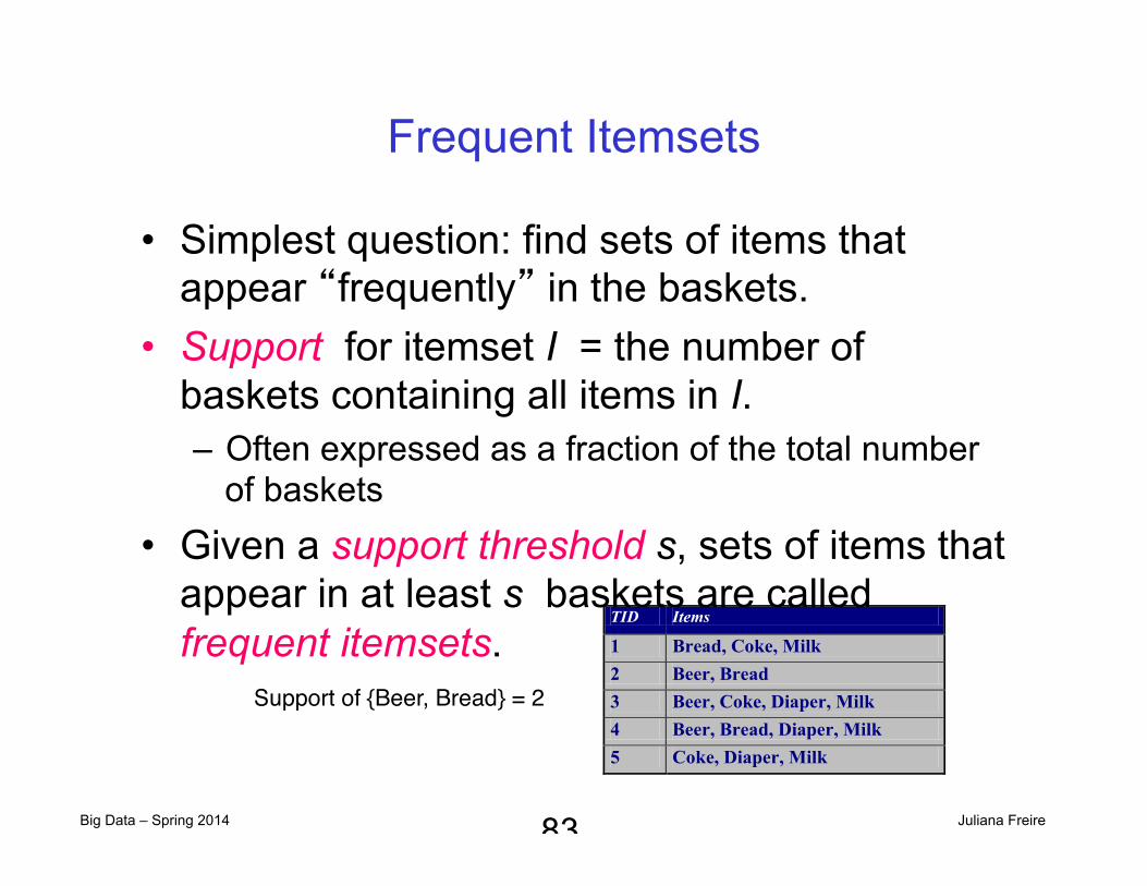
Frequent Itemsets
• Simplest question: find sets of items that appear “frequently” in the baskets.
• Support for itemset I = the number of baskets containing all items in I. – Often expressed as a fraction of the total number
of baskets • Given a support threshold s, sets of items that
appear in at least s baskets are called frequent itemsets.
83
� Simplest question: Find sets of items that appear together “frequently” in baskets
� Support for itemset I: Number of baskets containing all items in I � Often expressed as a fraction
of the total number of baskets � Given a support threshold s,
then sets of items that appear in at least s baskets are called frequent itemsets
1/10/2013 Jure Leskovec, Stanford CS246: Mining Massive Datasets, http://cs246.stanford.edu 9
TID Items
1 Bread, Coke, Milk
2 Beer, Bread
3 Beer, Coke, Diaper, Milk
4 Beer, Bread, Diaper, Milk
5 Coke, Diaper, Milk
Support of {Beer, Bread} = 2
Support of {Beer, Bread} = 2"

Big Data – Spring 2014 Juliana Freire
Association Rules
• If-then rules about the contents of baskets. • {i1, i2,…,ik} → j means: “if a basket contains
all of i1,…,ik then it is likely to contain j.” • Confidence of this association rule is the
probability of j given i1,…,ik.
84
11
� Association Rules: If-then rules about the contents of baskets
� {i1, i2,…,ik} ĺ�M means: “if a basket contains all of i1,…,ik then it is likely to contain j”
� In practice there are many rules, want to find significant/interesting ones!
� Confidence of this association rule is the probability of j given I = {i1,…,ik}
)support(
)support()conf(IjIjI �
o
1/10/2013 Jure Leskovec, Stanford CS246: Mining Massive Datasets, http://cs246.stanford.edu
Big Data – Spring 2014 Juliana Freire
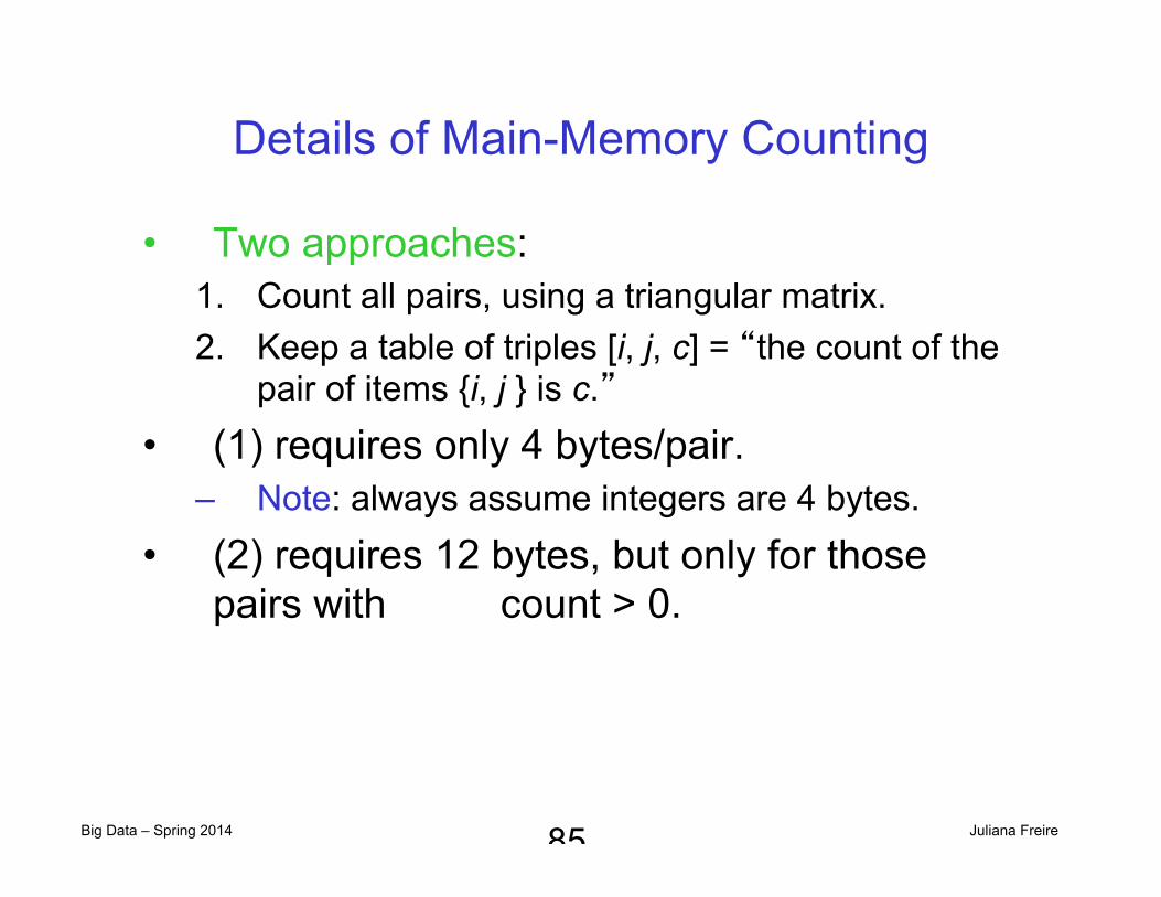
Details of Main-Memory Counting
• Two approaches: 1. Count all pairs, using a triangular matrix. 2. Keep a table of triples [i, j, c] = “the count of the
pair of items {i, j } is c.” • (1) requires only 4 bytes/pair.
– Note: always assume integers are 4 bytes.
• (2) requires 12 bytes, but only for those pairs with count > 0.
85
Big Data – Spring 2014 Juliana Freire
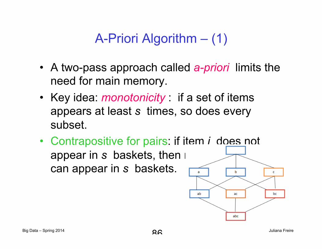
A-Priori Algorithm – (1)
• A two-pass approach called a-priori limits the need for main memory.
• Key idea: monotonicity : if a set of items appears at least s times, so does every subset.
• Contrapositive for pairs: if item i does not appear in s baskets, then no pair including i can appear in s baskets.
86
� A two-pass approach called a-priori limits the need for main memory
� Key idea: monotonicity � If a set of items I appears at
least s times, so does every subset J of I. � Contrapositive for pairs:
If item i does not appear in s baskets, then no pair including i can appear in s baskets
1/10/2013 Jure Leskovec, Stanford CS246: Mining Massive Datasets, http://cs246.stanford.edu 30
Big Data – Spring 2014 Juliana Freire
Association Rules: Not enough memory
• Counting for candidates C2 requires a lot of memory -- O(n2)
• Can we do better? • PCY: In pass 1, there is a lot of memory left,
leverage that to help with pass 2 – Maintain a hash table with as many buckets as fit in
memory – Keep count for each bucket into which pairs of items
are hashed • Just the count, not the pairs!
• Multistage improves PCY
87
Big Data – Spring 2014 Juliana Freire 88
Other Algorithms
• Random • SON – for mapreduce
Big Data – Spring 2014 Juliana Freire
Three Essential Techniques for Similar Documents
1. When the sets are so large or so many that they cannot fit in main memory.
2. Or, when there are so many sets that comparing all pairs of sets takes too much time.
3. Or both.
Big Data – Spring 2014 Juliana Freire
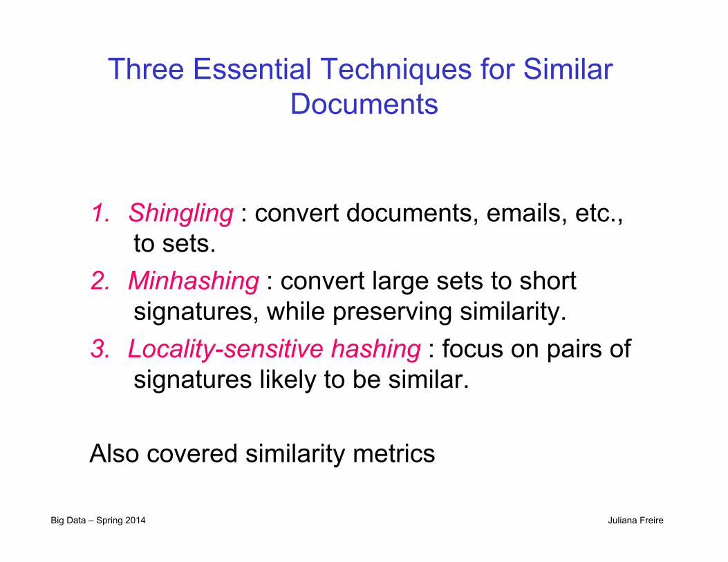
Three Essential Techniques for Similar Documents
1. Shingling : convert documents, emails, etc., to sets.
2. Minhashing : convert large sets to short signatures, while preserving similarity.
3. Locality-sensitive hashing : focus on pairs of signatures likely to be similar.
Also covered similarity metrics
Big Data – Spring 2014 Juliana Freire
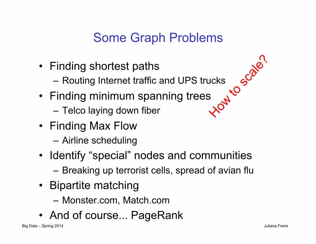
Some Graph Problems
• Finding shortest paths – Routing Internet traffic and UPS trucks
• Finding minimum spanning trees – Telco laying down fiber
• Finding Max Flow – Airline scheduling
• Identify “special” nodes and communities – Breaking up terrorist cells, spread of avian flu
• Bipartite matching – Monster.com, Match.com
• And of course... PageRank
Big Data – Spring 2014 Juliana Freire
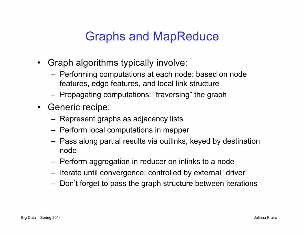
Graphs and MapReduce
• Graph algorithms typically involve: – Performing computations at each node: based on node
features, edge features, and local link structure – Propagating computations: “traversing” the graph
• Generic recipe: – Represent graphs as adjacency lists – Perform local computations in mapper – Pass along partial results via outlinks, keyed by destination
node – Perform aggregation in reducer on inlinks to a node – Iterate until convergence: controlled by external “driver” – Don’t forget to pass the graph structure between iterations
Big Data – Spring 2014 Juliana Freire
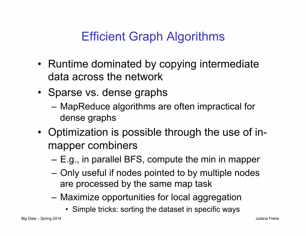
Efficient Graph Algorithms
• Runtime dominated by copying intermediate data across the network
• Sparse vs. dense graphs – MapReduce algorithms are often impractical for
dense graphs • Optimization is possible through the use of in-
mapper combiners – E.g., in parallel BFS, compute the min in mapper – Only useful if nodes pointed to by multiple nodes
are processed by the same map task – Maximize opportunities for local aggregation
• Simple tricks: sorting the dataset in specific ways
Big Data – Spring 2014 Juliana Freire
Alternatives to MapReduce
• MapReduce is not suitable for applications that re-use a working data set across multiple parallel operations
• A number of alternative approaches have been proposed: – Twister – Spark – Pregel – Haloop