Bidirectional Recurrent Convolutional Networksfor Multi-Frame Super-Resolution

Yan Huang1 Wei Wang1 Liang Wang1,2

1Center for Research on Intelligent Perception and ComputingNational Laboratory of Pattern Recognition

2Center for Excellence in Brain Science and Intelligence TechnologyInstitute of Automation, Chinese Academy of Sciences{yhuang, wangwei, wangliang}@nlpr.ia.ac.cn

Abstract

Super resolving a low-resolution video is usually handled by either single-imagesuper-resolution (SR) or multi-frame SR. Single-Image SR deals with each videoframe independently, and ignores intrinsic temporal dependency of video frameswhich actually plays a very important role in video super-resolution. Multi-FrameSR generally extracts motion information, e.g., optical flow, to model the temporaldependency, which often shows high computational cost. Considering that recur-rent neural networks (RNNs) can model long-term contextual information of tem-poral sequences well, we propose a bidirectional recurrent convolutional networkfor efficient multi-frame SR. Different from vanilla RNNs, 1) the commonly-usedrecurrent full connections are replaced with weight-sharing convolutional con-nections and 2) conditional convolutional connections from previous input layersto the current hidden layer are added for enhancing visual-temporal dependencymodelling. With the powerful temporal dependency modelling, our model cansuper resolve videos with complex motions and achieve state-of-the-art perfor-mance. Due to the cheap convolution operations, our model has a low compu-tational complexity and runs orders of magnitude faster than other multi-framemethods.

1 Introduction

Since large numbers of high-definition displays have sprung up, generating high-resolution videosfrom previous low-resolution contents, namely video super-resolution (SR), is under great demand.Recently, various methods have been proposed to handle this problem, which can be classified intotwo categories: 1) single-image SR [10, 5, 9, 8, 12, 25, 23] super resolves each of the video framesindependently, and 2) multi-frame SR [13, 17, 3, 2, 14, 13] models and exploits temporal dependencyamong video frames, which is usually considered as an essential component of video SR.

Existing multi-frame SR methods generally model the temporal dependency by extracting subpixelmotions of video frames, e.g., estimating optical flow based on sparse prior integration or variationregularity [2, 14, 13]. But such accurate motion estimation can only be effective for video sequenceswhich contain small motions. In addition, the high computational cost of these methods limits thereal-world applications. Several solutions have been explored to overcome these issues by avoidingthe explicit motion estimation [21, 16]. Unfortunately, they still have to perform implicit motionestimation to reduce temporal aliasing and achieve resolution enhancement when large motions areencountered.

Given the fact that recurrent neural networks (RNNs) can well model long-term contextual infor-mation for video sequence, we propose a bidirectional recurrent convolutional network (BRCN)

1

to efficiently learn the temporal dependency for multi-frame SR. The proposed network exploitsthree convolutions. 1) Feedforward convolution models visual spatial dependency between a low-resolution frame and its high-resolution result. 2) Recurrent convolution connects the hidden layersof successive frames to learn temporal dependency. Different from the commonly-used full recurrentconnection in vanilla RNNs, it is a weight-sharing convolutional connection here. 3) Conditionalconvolution connects input layers at the previous timestep to the current hidden layer, to further en-hance visual-temporal dependency modelling. To simultaneously consider the temporal dependencyfrom both previous and future frames, we exploit a forward recurrent network and a backward re-current network, respectively, and then combine them together for the final prediction. We apply theproposed model to super resolve videos with complex motions. The experimental results demon-strate that the model can achieve state-of-the-art performance, as well as orders of magnitude fasterspeed than other multi-frame SR methods.

Our main contributions can be summarized as follows. We propose a bidirectional recurrent con-volutional network for multi-frame SR, where the temporal dependency can be efficiently modelledby bidirectional recurrent and conditional convolutions. It is an end-to-end framework which doesnot need pre-/post-processing. We achieve better performance and faster speed than existing multi-frame SR methods.

2 Related Work

We will review the related work from the following prospectives.

Single-Image SR. Irani and Peleg [10] propose the primary work for this problem, followed byFreeman et al. [8] studying this problem in a learning-based way. To alleviate high computationalcomplexity, Bevilacqua et al. [4] and Chang et al. [5] introduce manifold learning techniques whichcan reduce the required number of image patch exemplars. For further acceleration, Timofte et al.[23] propose the anchored neighborhood regression method. Yang et al. [25] and Zeyde et al. [26]exploit compressive sensing to encode image patches with a compact dictionary and obtain sparserepresentations. Dong et al. [6] learn a convolutional neural network for single-image SR whichachieves the current state-of-the-art result. In this work, we focus on multi-frame SR by modellingtemporal dependency in video sequences.

Multi-Frame SR. Baker and Kanade [2] extract optical flow to model the temporal dependency invideo sequences for video SR. Then, various improvements [14, 13] around this work are exploredto better handle visual motions. However, these methods suffer from the high computational costdue to the motion estimation. To deal with this problem, Protter et al. [16] and Takeda et al. [21]avoid motion estimation by employing nonlocal mean and 3D steering kernel regression. In thiswork, we propose bidirectional recurrent and conditional convolutions as an alternative to modeltemporal dependency and achieve faster speed.

3 Bidirectional Recurrent Convolutional Network

3.1 Formulation

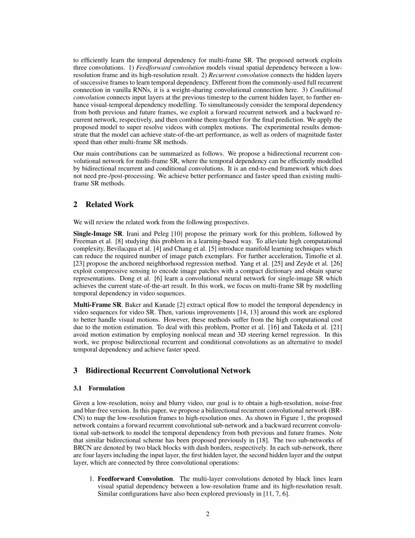
Given a low-resolution, noisy and blurry video, our goal is to obtain a high-resolution, noise-freeand blur-free version. In this paper, we propose a bidirectional recurrent convolutional network (BR-CN) to map the low-resolution frames to high-resolution ones. As shown in Figure 1, the proposednetwork contains a forward recurrent convolutional sub-network and a backward recurrent convolu-tional sub-network to model the temporal dependency from both previous and future frames. Notethat similar bidirectional scheme has been proposed previously in [18]. The two sub-networks ofBRCN are denoted by two black blocks with dash borders, respectively. In each sub-network, thereare four layers including the input layer, the first hidden layer, the second hidden layer and the outputlayer, which are connected by three convolutional operations:

1. Feedforward Convolution. The multi-layer convolutions denoted by black lines learnvisual spatial dependency between a low-resolution frame and its high-resolution result.Similar configurations have also been explored previously in [11, 7, 6].

2

𝑿𝒊−𝟏 𝑿𝒊 𝑿𝒊+𝟏

𝑿𝒊+𝟏 𝑿𝒊 𝑿𝒊−𝟏

⋯

⋯

⋯

⋯

⋯

⋯

⋯

⋯

Backward sub-network

Forward sub-network

Input layer (low-resolution frame)

Output layer (high-resolution frame)

First hidden layer

Second hidden layer

Second hidden layer

First hidden layer

Input layer (low-resolution frame)

: Feedforward convolution : Recurrent convolution : Conditional convolution

Figure 1: The proposed bidirectional recurrent convolutional network (BRCN).

2. Recurrent Convolution. The convolutions denoted by blue lines aim to model long-termtemporal dependency across video frames by connecting adjacent hidden layers of suc-cessive frames, where the current hidden layer is conditioned on the hidden layer at theprevious timestep. We use the recurrent convolution in both forward and backward sub-networks. Such bidirectional recurrent scheme can make full use of the forward and back-ward temporal dynamics.

3. Conditional Convolution. The convolutions denoted by red lines connect input layer atthe previous timestep to the current hidden layer, and use previous inputs to provide long-term contextual information. They enhance visual-temporal dependency modelling withthis kind of conditional connection.

We denote the frame sets of a low-resolution video1 X as {Xi}i=1,2,...,T , and infer the other threelayers as follows.

First Hidden Layer. When inferring the first hidden layer Hf1 (Xi) (or Hb

1(Xi)) at the ith timestepin the forward (or backward) sub-network, three inputs are considered: 1) the current input layerXi connected by a feedforward convolution, 2) the hidden layer Hf

1 (Xi−1) (or Hb1(Xi+1)) at the

i−1th (or i+1th) timestep connected by a recurrent convolution, and 3) the input layer Xi−1 (orXi+1) at the i−1th (or i+1th) timestep connected by a conditional convolution.

Hf1 (Xi) = λ(Wf

v1 ∗Xi + Wfr1 ∗H

f1 (Xi−1) + Wf

t1 ∗Xi−1 + Bf1 )

Hb1(Xi) = λ(Wb

v1 ∗Xi + Wbr1 ∗H

b1(Xi+1) + Wb

t1 ∗Xi+1 + Bb1)

(1)

where Wfv1 (or Wb

v1 ) and Wft1 (or Wb

t1 ) represent the filters of feedforward and conditional con-volutions in the forward (or backward) sub-network, respectively. Both of them have the size ofc×fv1×fv1×n1, where c is the number of input channels, fv1 is the filter size and n1 is the numberof filters. Wf

r1 (or Wbr1 ) represents the filters of recurrent convolutions. Their filter size fr1 is set to

1 to avoid border effects. Bf1 (or Bb

1) represents biases. The activation function is the rectified linearunit (ReLu): λ(x)=max(0, x) [15]. Note that in Equation 1, the filter responses of recurrent and

1Note that we upscale each low-resolution frame in the sequence to the desired size with bicubic interpola-tion in advance.

3

1B

1A

1C0C

iX1iX

1iH iH

1iXiX

1 1( )f

iH X 1 ( )f

iH X

-dimensional

vector

(a) TRBM (b) BRCN

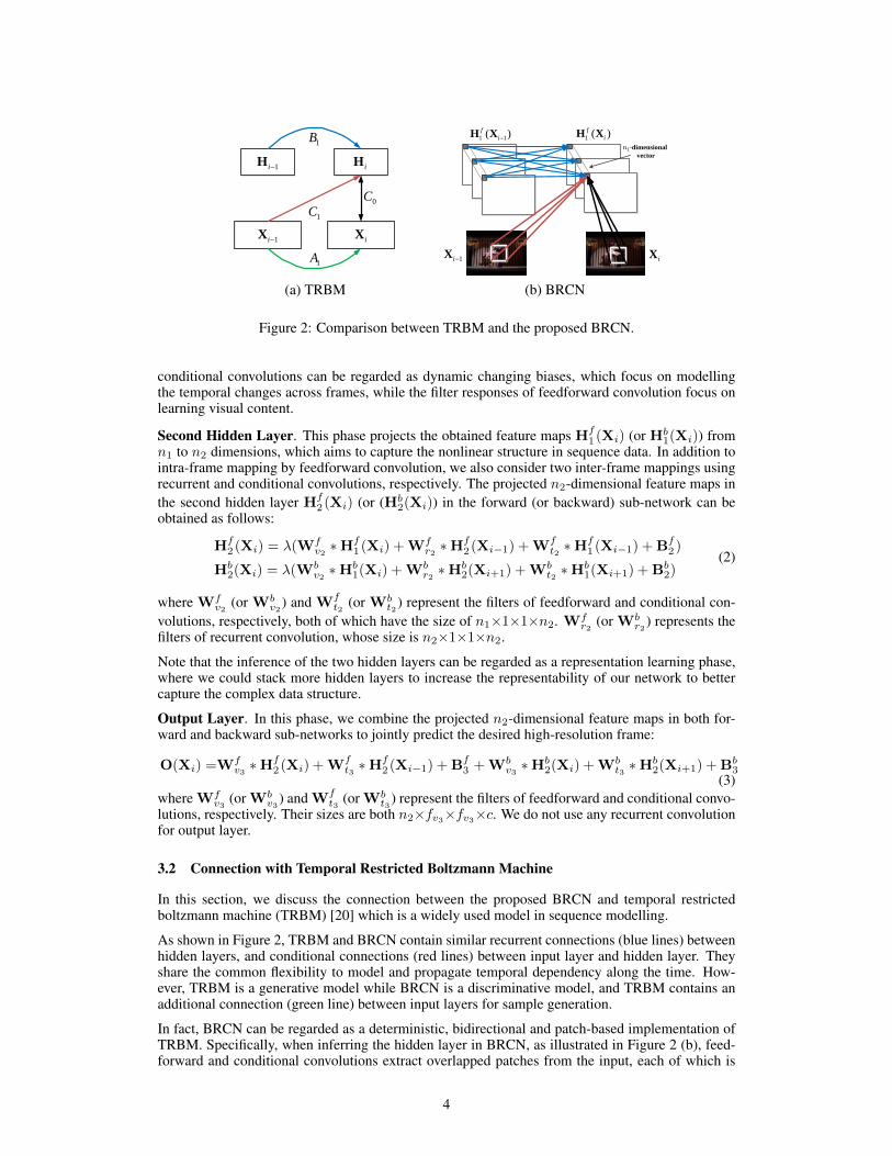
Figure 2: Comparison between TRBM and the proposed BRCN.

conditional convolutions can be regarded as dynamic changing biases, which focus on modellingthe temporal changes across frames, while the filter responses of feedforward convolution focus onlearning visual content.

Second Hidden Layer. This phase projects the obtained feature maps Hf1 (Xi) (or Hb

1(Xi)) fromn1 to n2 dimensions, which aims to capture the nonlinear structure in sequence data. In addition tointra-frame mapping by feedforward convolution, we also consider two inter-frame mappings usingrecurrent and conditional convolutions, respectively. The projected n2-dimensional feature maps inthe second hidden layer Hf

2 (Xi) (or (Hb2(Xi)) in the forward (or backward) sub-network can be

obtained as follows:

Hf2 (Xi) = λ(Wf

v2 ∗Hf1 (Xi) + Wf

r2 ∗Hf2 (Xi−1) + Wf

t2 ∗Hf1 (Xi−1) + Bf

2 )

Hb2(Xi) = λ(Wb

v2 ∗Hb1(Xi) + Wb

r2 ∗Hb2(Xi+1) + Wb

t2 ∗Hb1(Xi+1) + Bb

2)(2)

where Wfv2 (or Wb

v2 ) and Wft2 (or Wb

t2 ) represent the filters of feedforward and conditional con-volutions, respectively, both of which have the size of n1×1×1×n2. Wf

r2 (or Wbr2 ) represents the

filters of recurrent convolution, whose size is n2×1×1×n2.

Note that the inference of the two hidden layers can be regarded as a representation learning phase,where we could stack more hidden layers to increase the representability of our network to bettercapture the complex data structure.

Output Layer. In this phase, we combine the projected n2-dimensional feature maps in both for-ward and backward sub-networks to jointly predict the desired high-resolution frame:

O(Xi) =Wfv3 ∗H

f2 (Xi) + Wf

t3 ∗Hf2 (Xi−1) + Bf

3 + Wbv3 ∗H

b2(Xi) + Wb

t3 ∗Hb2(Xi+1) + Bb

3(3)

where Wfv3 (or Wb

v3 ) and Wft3 (or Wb

t3 ) represent the filters of feedforward and conditional convo-lutions, respectively. Their sizes are both n2×fv3×fv3

×c. We do not use any recurrent convolutionfor output layer.

3.2 Connection with Temporal Restricted Boltzmann Machine

In this section, we discuss the connection between the proposed BRCN and temporal restrictedboltzmann machine (TRBM) [20] which is a widely used model in sequence modelling.

As shown in Figure 2, TRBM and BRCN contain similar recurrent connections (blue lines) betweenhidden layers, and conditional connections (red lines) between input layer and hidden layer. Theyshare the common flexibility to model and propagate temporal dependency along the time. How-ever, TRBM is a generative model while BRCN is a discriminative model, and TRBM contains anadditional connection (green line) between input layers for sample generation.

In fact, BRCN can be regarded as a deterministic, bidirectional and patch-based implementation ofTRBM. Specifically, when inferring the hidden layer in BRCN, as illustrated in Figure 2 (b), feed-forward and conditional convolutions extract overlapped patches from the input, each of which is

4

fully connected to a n1-dimensional vector in the feature maps Hf1 (Xi). For recurrent convolution-

s, since each filter size is 1 and all the filters contain n1×n1 weights, a n1-dimensional vector inHf

1 (Xi) is fully connected to the corresponding n1-dimensional vector in Hf1 (Xi−1) at the previ-

ous time step. Therefore, the patch connections of BRCN are actually those of a “discriminative”TRBM. In other words, by setting the filter sizes of feedforward and conditional convolutions as thesize of the whole frame, BRCN is equivalent to TRBM.

Compared with TRBM, BRCN has the following advantages for handling the task of video super-resolution. 1) BRCN restricts the receptive field of original full connection to a patch rather than thewhole frame, which can capture the temporal change of visual details. 2) BRCN replaces all the fullconnections with weight-sharing convolutional ones, which largely reduces the computational cost.3) BRCN is more flexible to handle videos of different sizes, once it is trained on a fixed-size videodataset. Similar to TRBM, the proposed model can be generalized to other sequence modellingapplications, e.g., video motion modelling [22].

3.3 Network Learning

Through combining Equations 1, 2 and 3, we can obtain the desired prediction O(X ; Θ) from thelow-resolution video X , where Θ denotes the network parameters. Network learning proceeds byminimizing the Mean Square Error (MSE) between the predicted high-resolution video O(X ; Θ)and the groundtruth Y:

L = ‖O(X ; Θ)− Y‖2 (4)

via stochastic gradient descent. Actually, stochastic gradient descent is enough to achieve satisfyingresults, although we could exploit other optimization algorithms with more computational cost, e.g.,L-BFGS. During optimization, all the filter weights of recurrent and conditional convolutions areinitialized by randomly sampling from a Gaussian distribution with mean 0 and standard deviation0.001, whereas the filter weights of feedforward convolution are pre-trained on static images [6].Note that the pretraining step only aims to speed up training by providing a better parameter ini-tialization, due to the limited size of training set. This step can be avoided by alternatively using alarger scale dataset. We experimentally find that using a smaller learning rate (e.g., 1e−4) for theweights in the output layer is crucial to obtain good performance.

4 Experimental Results

To verify the effectiveness, we apply the proposed model to the task of video SR, and present bothquantitative and qualitative results as follows.

4.1 Datasets and Implementation Details

We use 25 YUV format video sequences2 as our training set, which have been widely used in manyvideo SR methods [13, 16, 21]. To enlarge the training set, model training is performed in a volume-based way, i.e., cropping multiple overlapped volumes from training videos and then regarding eachvolume as a training sample. During cropping, each volume has a spatial size of 32×32 and atemporal step of 10. The spatial and temporal strides are 14 and 8, respectively. As a result, wecan generate roughly 41,000 volumes from the original dataset. We test our model on a varietyof challenging videos, including Dancing, Flag, Fan, Treadmill and Turbine [19], which containcomplex motions with severe motion blur and aliasing. Note that we do not have to extract volumesduring testing, since the convolutional operation can scale to videos of any spatial size and temporalstep. We generate the testing dataset with the following steps: 1) using Gaussian filter with standarddeviation 2 to smooth each original frame, and 2) downsampling the frame by a factor of 4 withbicubic method3.

2http://www.codersvoice.com/a/webbase/video/08/152014/130.html.3Here we focus on the factor of 4, which is usually considered as the most difficult case in super-resolution.

5

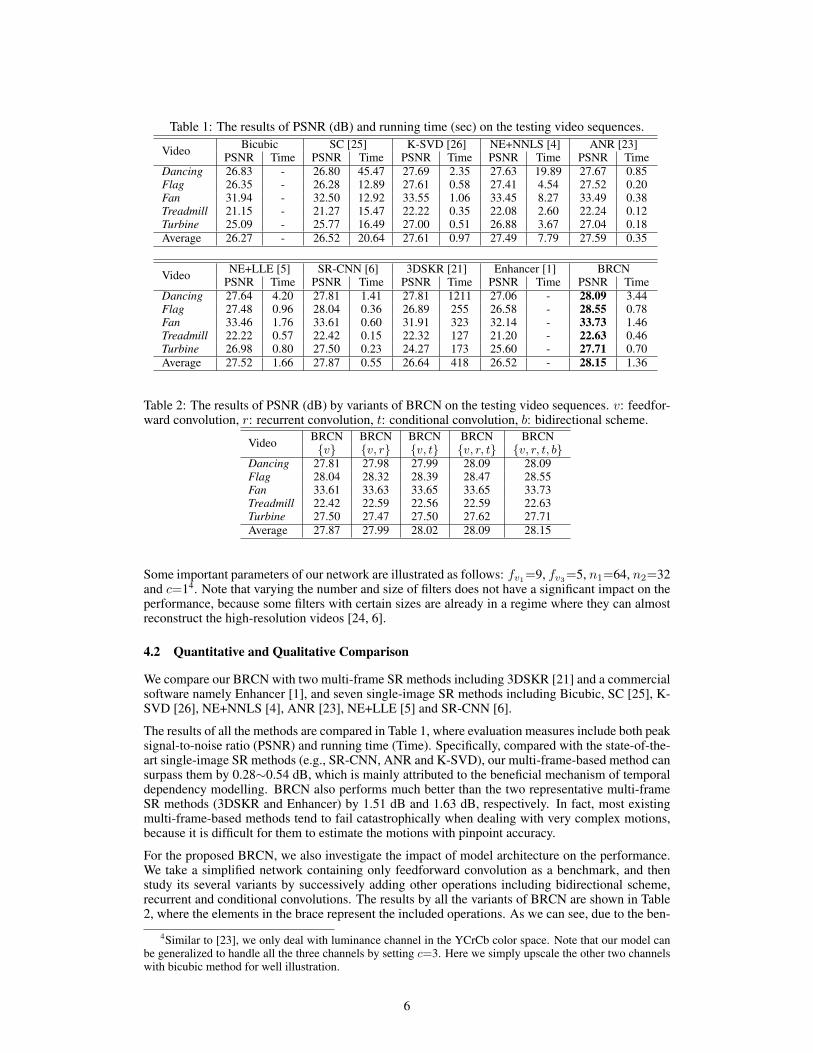
Table 1: The results of PSNR (dB) and running time (sec) on the testing video sequences.

Video Bicubic SC [25] K-SVD [26] NE+NNLS [4] ANR [23]PSNR Time PSNR Time PSNR Time PSNR Time PSNR Time

Dancing 26.83 - 26.80 45.47 27.69 2.35 27.63 19.89 27.67 0.85Flag 26.35 - 26.28 12.89 27.61 0.58 27.41 4.54 27.52 0.20Fan 31.94 - 32.50 12.92 33.55 1.06 33.45 8.27 33.49 0.38Treadmill 21.15 - 21.27 15.47 22.22 0.35 22.08 2.60 22.24 0.12Turbine 25.09 - 25.77 16.49 27.00 0.51 26.88 3.67 27.04 0.18Average 26.27 - 26.52 20.64 27.61 0.97 27.49 7.79 27.59 0.35

Video NE+LLE [5] SR-CNN [6] 3DSKR [21] Enhancer [1] BRCNPSNR Time PSNR Time PSNR Time PSNR Time PSNR Time

Dancing 27.64 4.20 27.81 1.41 27.81 1211 27.06 - 28.09 3.44Flag 27.48 0.96 28.04 0.36 26.89 255 26.58 - 28.55 0.78Fan 33.46 1.76 33.61 0.60 31.91 323 32.14 - 33.73 1.46Treadmill 22.22 0.57 22.42 0.15 22.32 127 21.20 - 22.63 0.46Turbine 26.98 0.80 27.50 0.23 24.27 173 25.60 - 27.71 0.70Average 27.52 1.66 27.87 0.55 26.64 418 26.52 - 28.15 1.36

Table 2: The results of PSNR (dB) by variants of BRCN on the testing video sequences. v: feedfor-ward convolution, r: recurrent convolution, t: conditional convolution, b: bidirectional scheme.

Video BRCN BRCN BRCN BRCN BRCN{v} {v, r} {v, t} {v, r, t} {v, r, t, b}

Dancing 27.81 27.98 27.99 28.09 28.09Flag 28.04 28.32 28.39 28.47 28.55Fan 33.61 33.63 33.65 33.65 33.73Treadmill 22.42 22.59 22.56 22.59 22.63Turbine 27.50 27.47 27.50 27.62 27.71Average 27.87 27.99 28.02 28.09 28.15

Some important parameters of our network are illustrated as follows: fv1=9, fv3=5, n1=64, n2=32and c=14. Note that varying the number and size of filters does not have a significant impact on theperformance, because some filters with certain sizes are already in a regime where they can almostreconstruct the high-resolution videos [24, 6].

4.2 Quantitative and Qualitative Comparison

We compare our BRCN with two multi-frame SR methods including 3DSKR [21] and a commercialsoftware namely Enhancer [1], and seven single-image SR methods including Bicubic, SC [25], K-SVD [26], NE+NNLS [4], ANR [23], NE+LLE [5] and SR-CNN [6].

The results of all the methods are compared in Table 1, where evaluation measures include both peaksignal-to-noise ratio (PSNR) and running time (Time). Specifically, compared with the state-of-the-art single-image SR methods (e.g., SR-CNN, ANR and K-SVD), our multi-frame-based method cansurpass them by 0.28∼0.54 dB, which is mainly attributed to the beneficial mechanism of temporaldependency modelling. BRCN also performs much better than the two representative multi-frameSR methods (3DSKR and Enhancer) by 1.51 dB and 1.63 dB, respectively. In fact, most existingmulti-frame-based methods tend to fail catastrophically when dealing with very complex motions,because it is difficult for them to estimate the motions with pinpoint accuracy.

For the proposed BRCN, we also investigate the impact of model architecture on the performance.We take a simplified network containing only feedforward convolution as a benchmark, and thenstudy its several variants by successively adding other operations including bidirectional scheme,recurrent and conditional convolutions. The results by all the variants of BRCN are shown in Table2, where the elements in the brace represent the included operations. As we can see, due to the ben-

4Similar to [23], we only deal with luminance channel in the YCrCb color space. Note that our model canbe generalized to handle all the three channels by setting c=3. Here we simply upscale the other two channelswith bicubic method for well illustration.

6

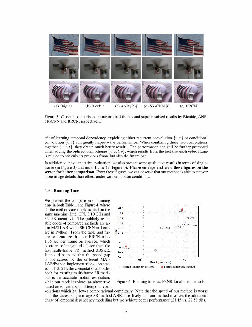
(a) Original (b) Bicubic (c) ANR [23] (d) SR-CNN [6] (e) BRCN

Figure 3: Closeup comparison among original frames and super resolved results by Bicubic, ANR,SR-CNN and BRCN, respectively.

efit of learning temporal dependency, exploiting either recurrent convolution {v, r} or conditionalconvolution {v, t} can greatly improve the performance. When combining these two convolutionstogether {v, r, t}, they obtain much better results. The performance can still be further promotedwhen adding the bidirectional scheme {v, r, t, b}, which results from the fact that each video frameis related to not only its previous frame but also the future one.

In addition to the quantitative evaluation, we also present some qualitative results in terms of single-frame (in Figure 3) and multi-frame (in Figure 5). Please enlarge and view these figures on thescreen for better comparison. From these figures, we can observe that our method is able to recovermore image details than others under various motion conditions.

4.3 Running Time

BRCN

3DSKR

SR-CNN

SC

NE+LLE ANR K-SVD

NE+NNLS

: multi-frame SR method : single-image SR method

Figure 4: Running time vs. PSNR for all the methods.

We present the comparison of runningtime in both Table 1 and Figure 4, whereall the methods are implemented on thesame machine (Intel CPU 3.10 GHz and32 GB memory). The publicly avail-able codes of compared methods are al-l in MATLAB while SR-CNN and oursare in Python. From the table and fig-ure, we can see that our BRCN takes1.36 sec per frame on average, whichis orders of magnitude faster than thefast multi-frame SR method 3DSKR.It should be noted that the speed gapis not caused by the different MAT-LAB/Python implementations. As stat-ed in [13, 21], the computational bottle-neck for existing multi-frame SR meth-ods is the accurate motion estimation,while our model explores an alternativebased on efficient spatial-temporal con-volutions which has lower computational complexity. Note that the speed of our method is worsethan the fastest single-image SR method ANR. It is likely that our method involves the additionalphase of temporal dependency modelling but we achieve better performance (28.15 vs. 27.59 dB).

7

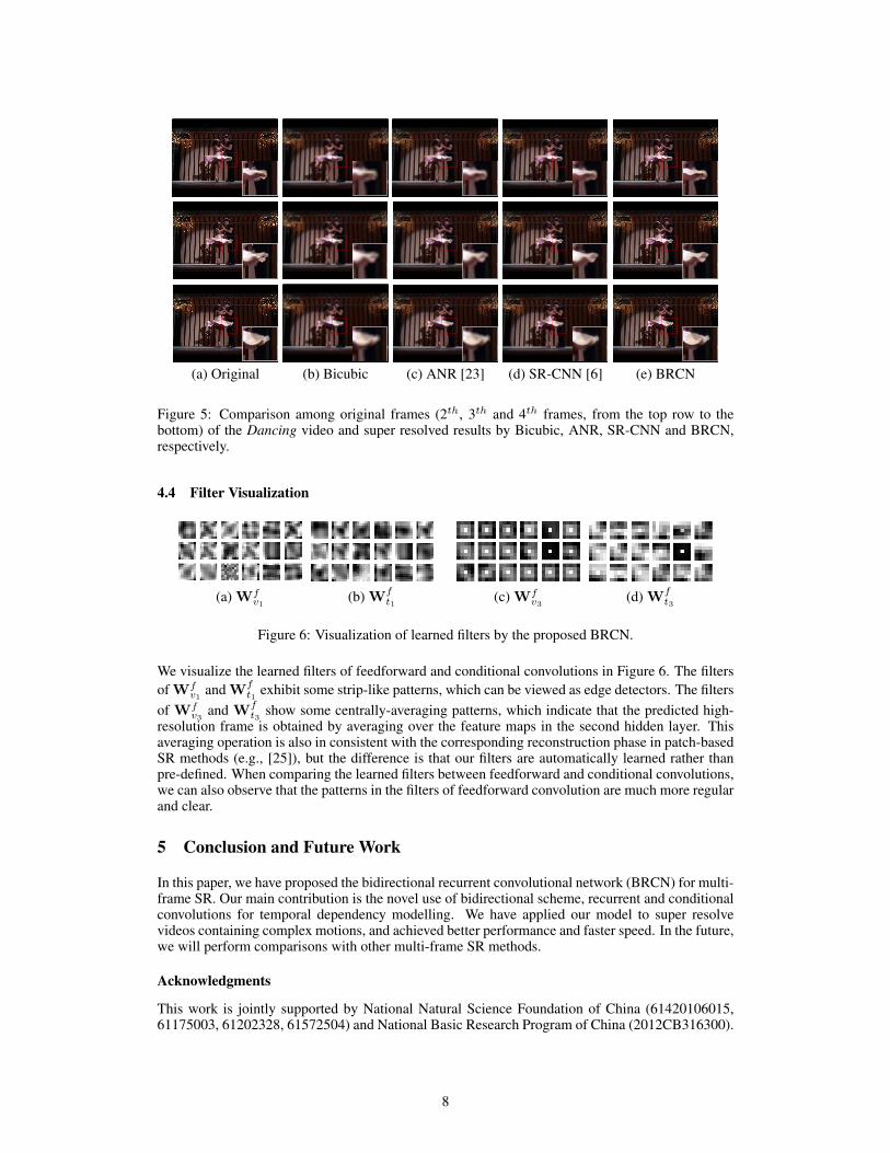
(a) Original (b) Bicubic (c) ANR [23] (d) SR-CNN [6] (e) BRCN

Figure 5: Comparison among original frames (2th, 3th and 4th frames, from the top row to thebottom) of the Dancing video and super resolved results by Bicubic, ANR, SR-CNN and BRCN,respectively.

4.4 Filter Visualization

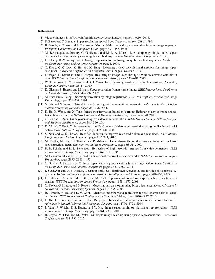
(a) Wfv1 (b) Wf

t1 (c) Wfv3 (d) Wf

t3

Figure 6: Visualization of learned filters by the proposed BRCN.

We visualize the learned filters of feedforward and conditional convolutions in Figure 6. The filtersof Wf

v1 and Wft1 exhibit some strip-like patterns, which can be viewed as edge detectors. The filters

of Wfv3 and Wf

t3 show some centrally-averaging patterns, which indicate that the predicted high-resolution frame is obtained by averaging over the feature maps in the second hidden layer. Thisaveraging operation is also in consistent with the corresponding reconstruction phase in patch-basedSR methods (e.g., [25]), but the difference is that our filters are automatically learned rather thanpre-defined. When comparing the learned filters between feedforward and conditional convolutions,we can also observe that the patterns in the filters of feedforward convolution are much more regularand clear.

5 Conclusion and Future Work

In this paper, we have proposed the bidirectional recurrent convolutional network (BRCN) for multi-frame SR. Our main contribution is the novel use of bidirectional scheme, recurrent and conditionalconvolutions for temporal dependency modelling. We have applied our model to super resolvevideos containing complex motions, and achieved better performance and faster speed. In the future,we will perform comparisons with other multi-frame SR methods.

Acknowledgments

This work is jointly supported by National Natural Science Foundation of China (61420106015,61175003, 61202328, 61572504) and National Basic Research Program of China (2012CB316300).

8

References

[1] Video enhancer. http://www.infognition.com/videoenhancer/, version 1.9.10. 2014.[2] S. Baker and T. Kanade. Super-resolution optical flow. Technical report, CMU, 1999.[3] B. Bascle, A. Blake, and A. Zisserman. Motion deblurring and super-resolution from an image sequence.

European Conference on Computer Vision, pages 571–582, 1996.[4] M. Bevilacqua, A. Roumy, C. Guillemot, and M.-L. A. Morel. Low-complexity single-image super-

resolution based on nonnegative neighbor embedding. British Machine Vision Conference, 2012.[5] H. Chang, D.-Y. Yeung, and Y. Xiong. Super-resolution through neighbor embedding. IEEE Conference

on Computer Vision and Pattern Recognition, page I, 2004.[6] C. Dong, C. C. Loy, K. He, and X. Tang. Learning a deep convolutional network for image super-

resolution. European Conference on Computer Vision, pages 184–199, 2014.[7] D. Eigen, D. Krishnan, and R. Fergus. Restoring an image taken through a window covered with dirt or

rain. IEEE International Conference on Computer Vision, pages 633–640, 2013.[8] W. T. Freeman, E. C. Pasztor, and O. T. Carmichael. Learning low-level vision. International Journal of

Computer Vision, pages 25–47, 2000.[9] D. Glasner, S. Bagon, and M. Irani. Super-resolution from a single image. IEEE International Conference

on Computer Vision, pages 349–356, 2009.[10] M. Irani and S. Peleg. Improving resolution by image registration. CVGIP: Graphical Models and Image

Processing, pages 231–239, 1991.[11] V. Jain and S. Seung. Natural image denoising with convolutional networks. Advances in Neural Infor-

mation Processing Systems, pages 769–776, 2008.[12] K. Jia, X. Wang, and X. Tang. Image transformation based on learning dictionaries across image spaces.

IEEE Transactions on Pattern Analysis and Machine Intelligence, pages 367–380, 2013.[13] C. Liu and D. Sun. On bayesian adaptive video super resolution. IEEE Transactions on Pattern Analysis

and Machine Intelligence, pages 346–360, 2014.[14] D. Mitzel, T. Pock, T. Schoenemann, and D. Cremers. Video super resolution using duality based tv-l 1

optical flow. Pattern Recognition, pages 432–441, 2009.[15] V. Nair and G. E. Hinton. Rectified linear units improve restricted boltzmann machines. International

Conference on Machine Learning, pages 807–814, 2010.[16] M. Protter, M. Elad, H. Takeda, and P. Milanfar. Generalizing the nonlocal-means to super-resolution

reconstruction. IEEE Transactions on Image Processing, pages 36–51, 2009.[17] R. R. Schultz and R. L. Stevenson. Extraction of high-resolution frames from video sequences. IEEE

Transactions on Image Processing, pages 996–1011, 1996.[18] M. Schusterand and K. K. Paliwal. Bidirectional recurrent neural networks. IEEE Transactions on Signal

Processing, pages 2673–2681, 1997.[19] O. Shahar, A. Faktor, and M. Irani. Space-time super-resolution from a single video. IEEE Conference

on Computer Vision and Pattern Recognition, pages 3353–3360, 2011.[20] I. Sutskever and G. E. Hinton. Learning multilevel distributed representations for high-dimensional se-

quences. In International Conference on Artificial Intelligence and Statistics, pages 548–555, 2007.[21] H. Takeda, P. Milanfar, M. Protter, and M. Elad. Super-resolution without explicit subpixel motion esti-

mation. IEEE Transactions on Image Processing, pages 1958–1975, 2009.[22] G. Taylor, G. Hinton, and S. Roweis. Modeling human motion using binary latent variables. Advances in

Neural Information Processing Systems, pages 448–455, 2006.[23] R. Timofte, V. De, and L. V. Gool. Anchored neighborhood regression for fast example-based super-

resolution. IEEE International Conference on Computer Vision, pages 1920–1927, 2013.[24] L. Xu, J. S. Ren, C. Liu, and J. Jia. Deep convolutional neural network for image deconvolution. In

Advances in Neural Information Processing Systems, pages 1790–1798, 2014.[25] J. Yang, J. Wright, T. S. Huang, and Y. Ma. Image super-resolution via sparse representation. IEEE

Transactions on Image Processing, pages 2861–2873, 2010.[26] R. Zeyde, M. Elad, and M. Protte. On single image scale-up using sparse-representations. Curves and

Surfaces, pages 711–730, 2012.

9