IN THE FIELD OF TECHNOLOGYDEGREE PROJECT INDUSTRIAL ENGINEERING AND MANAGEMENTAND THE MAIN FIELD OF STUDYINDUSTRIAL MANAGEMENT,SECOND CYCLE, 30 CREDITS

, STOCKHOLM SWEDEN 2019

Bid Forecasting in Public Procurement

KARIM STITI

SHIH JUNG YAPE

KTH ROYAL INSTITUTE OF TECHNOLOGYSCHOOL OF INDUSTRIAL ENGINEERING AND MANAGEMENT

This page is intentionally left blank

SE-100 44 STOCKHOLM

Bid Forecasting in Public Procurement

by

Karim Stiti Shih Jung Yape

Master of Science Thesis TRITA-ITM-EX 2019:446

KTH Industrial Engineering and Management

Industrial Management

SE-100 44 STOCKHOLM

Budgivningsmodeller i Offentliga Upphandlingar

av

Karim Stiti Shih Jung Yape

Examensarbete TRITA-ITM-EX 2019:446

KTH Industriell teknik och management

Industriell ekonomi och organisation

Keywords: Bidding in public procurement, Count data regression, Economically most advantageous tenders, Lowest price tenders, Machine learning, Multiple linear regression, Non-parametric bootstrap, Position performance coefficient, Sealed-bid auctions, Stochastic dominance, Support vector regression.

Master of Science Thesis

TRITA-ITM-EX 2019:446

Abstract

Public procurement amounts to a significant part of Sweden's GDP. Nevertheless, it is an

overlooked sector characterized by low digitization and inefficient competition where bids are

not submitted based on proper mathematical tools. This Thesis seeks to create a structured

approach to bidding in cleaning services by determining factors affecting the participation and

pricing decision of potential buyers. Furthermore, we assess price prediction by comparing

multiple linear regression models (MLR) to support vector regression (SVR). In line with

previous research in the construction sector, we find significance for several factors such as

project duration, location and type of contract on the participation decision in the cleaning

sector. One notable deviant is that we do not find contract size to have an impact on the pricing

decision. Surprisingly, the performance of MLR are comparable to more advanced SVR

models. Stochastic dominance tests on price performance concludes that experienced bidders

perform better than their inexperienced counterparts and companies place more competitive

bids in lowest price tenders compared to economically most advantageous tenders (EMAT)

indicating that EMAT tenders are regarded as unstructured. However, no significance is found

for larger actors performing better in bidding than smaller companies.

Examiner

Pontus Braunerhjelm Comissioner

Tendium AB

Supervisor

Almas Heshmati Contact person

Farzad Khoshnoud

Approved

2019-06-14

Bid Forecasting in Public Procurement

Karim Stiti

Shih Jung Yape

Nyckelord: Budgivningsmodeller I offentliga upphandlingar, Ekonomiskt mest fördelaktiga anbud, Förseglade auktioner, Lägsta-pris anbud, Maskininlärning, Multipel linjär regression.

Examensarbete

TRITA-ITM-EX 2019:446

Godkänt

2019-06-14

Sammanställning

Examinator

Pontus Braunerhjelm

lm

Uppdragsgivare

Tendium AB

Handledare

Almas Heshmati Kontaktperson

Farzad Khoshnoud

Budgivningmodeller i Offentliga Upphandlingar

Karim Stiti

Shih Jung Yape

Offentliga upphandlingar utgör en signifikant del av Sveriges BNP. Trots detta är det en

förbisedd sektor som karakteriseras av låg digitalisering och ineffektiv konkurrens där bud

läggs baserat på intuition snarare än matematiska modeller. Denna avhandling ämnar skapa

ett strukturerat tillvägagångssätt för budgivning inom städsektorn genom att bestämma

faktorer som påverkar deltagande och prissättning. Vidare undersöker vi

prisprediktionsmodeller genom att jämföra multipel linjära regressionsmodeller med en

maskininlärningsmetod benämnd support vector regression. I enlighet med tidigare

forskning i byggindustrin finner vi att flera faktorer som typ av kontrakt, projekttid och

kontraktsplats har en statistisk signifikant påverkan på deltagande i kontrakt i städindustrin.

En anmärkningsvärd skillnad är att kontraktsvärdet inte påverkar prissättning som tidigare

forskning visat i andra områden. För prisprediktionen är det överraskande att den enklare

linjära regressionsmodellen presterar jämlikt till den mer avancerade

maskininlärningsmodellen. Stokastisk dominanstest visar att erfarna företag har en bättre

precision i sin budgivning än mindre erfarna företag. Därtill lägger företag överlag mer

konkurrenskraftiga bud i kontrakt där kvalitetsaspekter tas i beaktning utöver priset. Vilket

kan indikera att budgivare upplever dessa kontrakt som mindre strukturerade. Däremot

finner vi inger signifikant skillnad mellan större och mindre företag i denna bemärkning.

This page is intentionally left blank

Acknowledgements

We would like to express our deep and sincere gratitude to our thesis advisor Pro-fessor Almas Heshmati for his continuous support and guidance within the field ofstatistical analysis. His broad experience and expertise was valuable for us throughdifferent part of our thesis. We could not have imagined a more suitable candi-date in counselling us than Professor Almas. Beside our advisor, we would also liketo thank the people who helped us in Tendium, mainly Farzad Khousnoud, PeterVesterberg and Tim Lachmann. Together with Farzad we developed the idea offorecasting public procurement in the Swedish cleaning industry. Peter and Timprovided insight in data handling and model constructions which was helpful for theend result.

Finally, we gratefully acknowledge the support and continuous love of our parents.Their influence throughout our education is what have driven our passion and thecompletion of this thesis.

Jung Yape and Karim StitiStockholm, June 2019

i

Table of Contents

1 Introduction 11.1 Background . . . . . . . . . . . . . . . . . . . . . . . . . . . . . . . . 11.2 Purpose . . . . . . . . . . . . . . . . . . . . . . . . . . . . . . . . . . 31.3 Problem Formulation . . . . . . . . . . . . . . . . . . . . . . . . . . . 31.4 Sustainability Aspect . . . . . . . . . . . . . . . . . . . . . . . . . . . 41.5 Scope . . . . . . . . . . . . . . . . . . . . . . . . . . . . . . . . . . . 41.6 Report Structure . . . . . . . . . . . . . . . . . . . . . . . . . . . . . 5

2 Previous Research in Sealed Bid Auctions 62.1 Measuring Tender Participation . . . . . . . . . . . . . . . . . . . . . 6

2.1.1 Probability of Winning Tenders . . . . . . . . . . . . . . . . . 62.1.2 Determining Number of Participants in Tenders . . . . . . . . 72.1.3 Factors Influencing the Bid/No Bid Decision . . . . . . . . . . 8

2.2 Price Prediction Models in Sealed Bid Auctions . . . . . . . . . . . . 92.2.1 Predicting Bid Prices Using Statistical Models and Machine

Learning . . . . . . . . . . . . . . . . . . . . . . . . . . . . . . 102.3 Assessing EMAT tenders . . . . . . . . . . . . . . . . . . . . . . . . . 122.4 Green Public Procurement - Environmental Quality Criteria . . . . . 13

3 Empirical Framework 163.1 Multiple Linear Regression Analysis . . . . . . . . . . . . . . . . . . . 163.2 Model Validation . . . . . . . . . . . . . . . . . . . . . . . . . . . . . 17

3.2.1 Multicollinearity . . . . . . . . . . . . . . . . . . . . . . . . . 173.2.2 Residual Diagnostics . . . . . . . . . . . . . . . . . . . . . . . 183.2.3 Variable Transforms . . . . . . . . . . . . . . . . . . . . . . . 19

3.3 Model Selection . . . . . . . . . . . . . . . . . . . . . . . . . . . . . . 203.3.1 Selective Criteria . . . . . . . . . . . . . . . . . . . . . . . . . 203.3.2 K-fold Cross-Validation . . . . . . . . . . . . . . . . . . . . . . 21

3.4 Poisson Regression Models . . . . . . . . . . . . . . . . . . . . . . . . 213.4.1 Negative Binomial Regression . . . . . . . . . . . . . . . . . . 23

3.5 Support Vector Regression . . . . . . . . . . . . . . . . . . . . . . . . 253.6 Probit Regression . . . . . . . . . . . . . . . . . . . . . . . . . . . . . 263.7 Stochastic Dominance . . . . . . . . . . . . . . . . . . . . . . . . . . 273.8 Confidence Intervals Using Non-Parametric Bootstrap . . . . . . . . . 273.9 Joint Distribution Function with Position Performance . . . . . . . . 293.10 Other Statistical Models . . . . . . . . . . . . . . . . . . . . . . . . . 30

3.10.1 Chi-Square Test . . . . . . . . . . . . . . . . . . . . . . . . . . 30

ii

4 Data and Methodology 314.1 Data Collection and Limitations . . . . . . . . . . . . . . . . . . . . . 314.2 Variable Description . . . . . . . . . . . . . . . . . . . . . . . . . . . 324.3 Competitors Affect On Price . . . . . . . . . . . . . . . . . . . . . . . 344.4 Assessing Tender Participants . . . . . . . . . . . . . . . . . . . . . . 344.5 Predict Price Performance . . . . . . . . . . . . . . . . . . . . . . . . 36

4.5.1 Comparing Multiple Linear Regression and Support VectorRegression . . . . . . . . . . . . . . . . . . . . . . . . . . . . . 36

4.5.2 Inference for experience, size and tendering method with Stochas-tic Dominance . . . . . . . . . . . . . . . . . . . . . . . . . . . 38

4.6 Assessing Quality Performance . . . . . . . . . . . . . . . . . . . . . . 38

5 Results 405.1 Bid/no Bid Decision . . . . . . . . . . . . . . . . . . . . . . . . . . . 40

5.1.1 Number of Bidder’s Effect on Price . . . . . . . . . . . . . . . 405.1.2 Fitting a Distribution the Participation Data . . . . . . . . . . 415.1.3 Factors Contributing to Participants With Regression . . . . . 455.1.4 Impact of Environmental Criteria on Participation . . . . . . . 515.1.5 Bid/No Bid Decision for Individual Participants . . . . . . . . 51

5.2 Predicting Price . . . . . . . . . . . . . . . . . . . . . . . . . . . . . . 535.2.1 Factors Affecting Pricing . . . . . . . . . . . . . . . . . . . . . 535.2.2 Comparing SVR And MLR Models for Price Prediction . . . . 545.2.3 Price Range with Non-parametric Bootstrap . . . . . . . . . . 565.2.4 Stochastic Dominance for Spread . . . . . . . . . . . . . . . . 585.2.5 Price Performance with Spread Variable . . . . . . . . . . . . 60

5.3 Competitor Performance in EMAT tenders . . . . . . . . . . . . . . . 61

6 Analysis of Results 636.1 Number of Competitors . . . . . . . . . . . . . . . . . . . . . . . . . 636.2 Bid/No Bid Logistic Regression . . . . . . . . . . . . . . . . . . . . . 666.3 Predicting Price . . . . . . . . . . . . . . . . . . . . . . . . . . . . . . 66

6.3.1 Stochastic Dominance and Non-Parametric Bootstrap Analysis 686.4 Quantifying Quality . . . . . . . . . . . . . . . . . . . . . . . . . . . . 69

7 Conclusions 71

8 Suggestions for Future Research 73

Bibliography 74

Appendix 80A. Literature Review . . . . . . . . . . . . . . . . . . . . . . . . . . . 80

iii

B. Bid/No-Bid Probit Regression . . . . . . . . . . . . . . . . . . . . 81C. Diagnostics . . . . . . . . . . . . . . . . . . . . . . . . . . . . . . . 82D. Price Prediction . . . . . . . . . . . . . . . . . . . . . . . . . . . . 84

iv

1 Introduction

In this section public procurement auctions are introduced, the objectives and im-

plications of our thesis are described, the scope explained and finally we detail the

report structure.

1.1 Background

The purchase of goods and services by a public organization from external sources

is termed public procurement. It has a sizeable affect on world trade amounting to

more than 1.3 trillion euro each year. In EU it accounts for around 16 % of GDP

and during 2016 the EU put in new rules intended to open up the public procure-

ment market within Europe. The stated goal was to streamline processes and make

it easier for smaller companies to participate in the market (European Commission

2017). The total value of public procurement contracts in Sweden was estimated

to 683 billion SEK which is a 17 % share of GDP. In 2017, 18525 contracts were

announced and 39 % of those were in the construction sector (Upphandlingsmyn-

digheten 2019).

Public procurement contracts are awarded by Swedish local government in a process

known as sealed bid auctions meaning no bidder knows what the other participants

have bid (Upphandlingsmyndigheten 2019). This is a broadly used auction method

not only in public procurement but also in private procurement, especially in the

construction sector (Brook 2016).

There has been a steady decline from an already low level of the average number

of participants in public procurement auctions in Sweden, in particular the cleaning

industry. Today, there are on average 4.3 bidders per contract. It is the goal of the

Swedish government to increase competitiveness and make public procurement more

efficient (Upphandlingsmyndigheten 2019). The market is plagued by laws that

make the process static and inefficient which subsequently leads to inexperienced

parties winning auctions. Contracts where the winner is determined by combining

an assessment of quality with price have also not been effective (Inkopsradet 2016).

1

The bidding process in cleaning services in particular has been characterized by bids

under the recommended price winning. As a result, serious actors are electing not to

participate (Fastighetsfolket 2017). Part of the improvement process is to evaluate

how artificial intelligence can be used by the government in public procurement

to increase security and improve processing time. In addition, they aim to make

the market more transparent by providing access to more data (Regeringskansliet

2019).

We perform our analysis in this thesis by drawing on both existing literature directly

from cleaning in public procurement and the construction industry. We believe this

paper contributes to the existing literature in several ways. Firstly, it provides an

updated look at factors affecting the bid/no bid and pricing decision of bidders in

public procurement cleaning using factors initially discovered in the construction

industry. Secondly, we find that linear models perform in line to more advanced

support vector regressions. Thirdly, using models that have not been applied to

public procurement before we show that the experience of the bidder is more im-

portant when it comes to performance in tenders than company size. This follows

as more frequent bidders perform better than less frequent bidders and have smaller

confidence intervals in their bids; indicating that with experience comes structure in

bidding. Finally, we show companies tend to bid more evenly in lowest price tenders

compared to EMAT tenders. All together, our results show that one can draw infer-

ence of bidding behaviour with straightforward mathematical models and as more

structured data is made available with time a complete bid forecasting model can

be built.

2

1.2 Purpose

The Swedish Upphandlingsmyndigheten is hoping to streamline and digitize the

public procurement sector in general and the cleaning services in particular. It is a

sector plagued by low competition and inefficiency. Our thesis seeks to understand

and improve the low participation rate in cleaning services’ tenders by contributing

to digitizing the sector. We do this by evaluating pricing models and participa-

tion models that will make the bidding easier and more transparent. In addition,

considering the perceived problems with economically most advantageous tenders

(EMAT), we also intend to study whether there is a difference in how companies

perform in EMAT in relation to lowest price tenders.

1.3 Problem Formulation

Considering the industry inefficiencies, an important question to pose is whether

there is in fact any structure to the bidding behavior of participants or if they act

randomly. This thesis will seek to understand whether models can be developed for

the behavior of competitors within the Swedish cleaning service industry and in that

case what models are best suited. The approach to these problems is to divide them

into two main areas of study: The bid/no bid decision of competitors and predicting

bid prices. To do this we must first determine factors that affect the decision-making

of companies in the sector, then we will explore whether simple linear regression

models or more advanced machine learning methods perform better.

Research Question 1 (RQ1): What factors contribute to companies bidding in

public procurement?

Research Question 2 (RQ2): What factors affect the pricing decision in public

procurement?

3

Research Question 3 (RQ3): Are multiple linear regression or support vector re-

gression models best suited for price prediction in public procurement?

Research Question 4 (RQ4): How does bidder performance differ in EMAT ten-

ders compared to lowest price tenders?

1.4 Sustainability Aspect

This paper will explore sustainability through the public procurement contracts that

are EMAT tenders. We will study these contracts to determine what impact the

quality criteria based on environmental factors has on participation. This results in

the following research question:

Research Question 5 (RQ5): Does participation increase or decrease when en-

vironmental quality criteria are included in EMAT tenders?

1.5 Scope

Our research will only focus on public procurement contracts in the cleaning services

sector in central and the south of Sweden from 2016-2019. Within the cleaning

sector we focused on sanitation and standard cleaning of floors and windows. For

price analysis, we only look at floor care. Some of the companies participating in

these tenders are not Swedish but no distinctions are made between Swedish and

foreign firms. Previous research presents numerous attributes that have an affect

on bidding in other sectors as well as in the cleaning industry. We limit our thesis

to those that are most quantifiable and are accessible to us from our database.

Limitations in the data will be further explored in section 4.1. The study methods

used will mainly consist of regression analysis but some inference will be drawn from

stochastic dominance and non-parametric bootstrapping.

4

1.6 Report Structure

The paper is organized as follows. Section 2.1 starts off by going trough research in

tender participation with section 2.1.3 in particular detailing findings when looking

at factors affecting the bid/no bid decision. Section 2.2 provides an overview of

existing literature pertaining to predicting bid prices and determinants of the pricing

decision. The literature review concludes with section 2.3 describing the difficulty in

judging economically most advantageous tenders and 2.4 that looks specifically at

the impact of environmental quality criteria. All of the mathematical models used

in this thesis are presented next. Section 4 then describes the data and details its

limitations as well as defining key variables. In addition, it is exhaustively explained

how we intend to apply the methods that have been introduced in section 3. We

outline each approach in the order they will be presented in the results section.

Results will be presented in section 5 for fitting tender participation into a known

distribution and the regression models. Price prediction model comparison and price

performance is shown next and we finally present the assessment of EMAT tenders.

Section 6 and 7 analyzes and concludes the results. Finally, suggestions for further

research are presented in section 8.

5

2 Previous Research in Sealed Bid Auctions

Using past research we hope to find good models that can be used for our thesis.

For tender participants there are some existing studies in public procurement for

cleaning services that we can build on. For price prediction and EMAT assessment

the research is more sparse and we seek studies in other sectors such as construc-

tion.

2.1 Measuring Tender Participation

2.1.1 Probability of Winning Tenders

Multiple and logistic regression can be applied in determining probabilities of win-

ning tenders. Data from one specific bidding firm in the Polish construction industry

allowed Malara and Mazurkiewcz (2012) to model the winning probability through

a binary logistic regression model. The binary response variable is partially deter-

mined by qualitative variables such as the type of tender, size of the procurer and

the presence of partner contractors, and partially by quantitative variables such as

number of competitors, lowest price bid and highest price bid.

Results in Malara and Mazurkiewcz (2012) model gave the suppliers either an output

of 0 as in loosing the tender or 1 as in winning the tender. Rounding between 0 and

1 are done accordingly with standard mathematical procedures. Although Malara

and Mazurkiewcz do not forecast any optimal bid range or optimal bid price, their

contribution could still be useful for this study. Their method of determining winning

probabilities can be incorporated in other auction bidding theories that both utilize

quality and price to find and optimal bid. Lastly, it is imperative to note that the

model Malara and Mazurkiewcz propose is restricted to one firm’s probability of

winning, which may not be satisfactory in a large competitive setting with many

actors.

Malara and Mazurkiewcz work is pertinent for this thesis, not due to their procedure

of measuring the probability of winning tenders, but rather for what factors that

6

could contribute firms to participate in tenders. Furthermore, their mathematical

theory could be of significance for this thesis since they apply binary regression

models well aligned with probit regression and the probability of a firm participating

in tenders.

2.1.2 Determining Number of Participants in Tenders

There have been varying results regarding the effect of number of participants on

the tender outcome. An analysis of the so called bid spread, defined in section 4.2,

in auctions did not show any significant effect by either number of competitors or

contract size (Drew et al. 2001). However, determining the number of participants

in a contract may be pertinent due to simple supply demand theory; the more

bidders in a contract, the harder it becomes for firms to profit and the cheaper

it becomes for buyers. Several studies have centered around understanding how

different factors affect the participation rate of contracts in different industries.

Augustin and Walter (2010) found in their study on operator changes that project

duration, i.e. longer contracts, usually increased the participation rate in contracts.

When studying competitive bidding Beck (2011) found that season was statistical

significant when describing the number of participants in tenders. Contracts starting

during summer or at the beginning of the year had lower participation rate than

contracts that started mid autumn or mid spring. Although indications that both

time and seasonal components might affect the amount of participants in contracts,

it is important to be critical. Influencing factors may vary for different industries

depending on the type of project, the risk firms undertake and the amount of capital

firms bind during a certain time period (Agerberg and Agren 2012).

A more explanatory procedure for determining number of participants in contracts

was presented by Vigren (2017). In his study, Vigren used count data regression

models to determine what contract characteristics that affected the number of bids

for public transport bus contracts. The main finding from the study was that most

contract features changed participation in tenders by around 0.1− 0.5 bidders. The

factors he looked at included, project duration, number of other tenders available,

geography, a firm’s current workload and whether the contract was evaluated based

7

on lowest price or economically most advantageous criteria. He compared ordinary

least-square to Poisson Regression, Generalized Poisson Regression, Truncated Pois-

son Regression and Truncated Generalized Poisson. The OLS regression performed

worse than the different Poisson models. In particular he found that project du-

ration increased the number of participants while tenders that are evaluated on

EMAT decrease the number of participants as with the number of other tenders

available to bid, possibly indicating that some firms have limited capacity to bid.

Finally, Vigren found that tenders with combined contracts did not affect the overall

participation.

Over the years the participation rate of contracts ranging from the timber industry

to the construction industry has been found to vary depending on factors such as

the type of project (Drew and Skitmore 2006; Athey et al. 2011), client relationship

(Bageis and Fortune 2009), project location (Azman 2014), project duration (Au-

gustin and Walter 2010) and project size (Al-Arjani 2002; Benjamin 1969; Drew and

Skitmore 2006; Lundberg et al. 2015). To further understand important attributes

that may contribute to the bidding participation rate, it is relevant to study factors’

influence on single firm’s bidding participation.

2.1.3 Factors Influencing the Bid/No Bid Decision

Numerous studies have been made on which factors that are most important when

assessing the bid/no bid decision and overall competitiveness for contracts in dif-

ferent sectors. One study in the construction industry, performed by Cheng et al.

(2010), indicated variables such as project size, type of project, time available for

tender preparation, current workload, expected number of competitors, tendering

method and project duration to be important for a firm’s decision to bid in a con-

tract (remaining factors in Cheng et. al. study are illustrated in table 21). In

comparison to other studies which uses various statistical models they implement

a questionnaire to determine important factors contributing to firms’ bid/no bid

decisions. Cheng et. al. gathered key influencing factors from renowned market

participants, weighed their relative importance within the industry and finally gave

them points that described factors’ significance to contracts. Ballesteros-Perez et

8

al. (2016) took a similar approach as Cheng where they focused on anticipating the

participation of individual bidders. They found that contract size was significant

and thus affected the likelihood of individual bidders to participate in contracts.

Furthermore, bidders that have not previously participated in a auction are impor-

tant to consider in tender forecasting models, since excluding them would limit the

predictive accuracy (Ballesteros-Perez et al. 2016)

Fu (2003) measured in his doctoral thesis the effect of contractor’s bidding expe-

riences on competitiveness in recurrent bidding. His work is pertinent in multi-

attribute tendering theory since he incorporates other important factors to assess

competitive bidding. Well aligned with Cheng et al. (2010) he studied how fac-

tors contributes to bid/no bid contract decision, Fu found that features such as

client relationship, a firm’s previous experience, project size and project location

to be important when determining competitiveness mainly within the construction

industry.

By comparing studies in the construction industry (Cheng et al. 2010; Fu 2003) and

public transport industry (Vigren 2017), there is a further strong indication that

common factors to assess in bid/no bid decision models are project size, project

location and the workload (in some studies called market conditions) of firms.

Conclusively, the number and identity of participants auctions in economics have

been challenging to forecast. There are few models that provide accurate solutions

or predictions, thus further strengthening the fact that the area of multi-attribute

auction theory and assessment of factors contributing to competitive bidding to be

a fairly unexplored field of study. In addition, there are no good models to predict

specific number of key competitors (Ballesteros-Perez et al. 2015).

2.2 Price Prediction Models in Sealed Bid Auctions

In this section we review past research to identify attributes that affect the pricing

decision of a bidder to use in our regression analysis. There have been several

studies in this area and Takano et al. (2018) categorized them into three buckets:

statistical models, multi-criteria utility models and artificial-intelligence (AI) based

9

models. We focus on statistical and AI models by presenting the results of previous

attempts to use machine learning and least-square regression to predict prices in

sealed bid auctions in procurement. In addition to these models we would also argue

the prevalence of models based on game theory. Friedman, a prominent researcher

in bidding theory, neglected these model arguing game theory models were only

functional when the number of bidders are predictable and few Friedman (1956), a

rare occurrence in this types of auctions.

2.2.1 Predicting Bid Prices Using Statistical Models and Machine Learn-

ing

Based on an extensive literature review it was found that factors affecting the bid

decision of companies in the construction sector can be categorized into seven ma-

jor groups; project characteristics, economic Characteristics, bidding characteris-

tics, contract Characteristics, owner characteristics, company characteristics and

opportunity Characteristics. Some of the most prominent attributes within these

categories were project size, investment risks, time for tender preparation, type of

contract, relationship with the owner, current workload and need for work (Polat

et al. 2016). The paper further compared a machine learning method called ar-

tificial neural network with least-square regression. They found that both models

performed equally with good predictive accuracy.

10

In one paper least-square regression was applied to forecast a bidding range. They

applied logistic regression and found a model with a very high model fit (Petrovski et

al. 2015). An advantage of this model is that it can easily take in to account several

factors that impact the bidding decision, both quantitative and qualitative.

Artificial intelligence tools have been used since the 1990s to tackle bidding problems.

Methods include artificial neural networks (Hegazy and Moselhi 1994; Li 1996), case-

based reasoning (Dikmen et al. 2007) and fuzzy set theory (Fayek 1998).

A paper that instead looks at itemized bids is Jung and Kim (2019) that provided a

forecasting model to using a machine learning approach called random forest method

to estimate bidding ranges with the help of random forest variable selection and

regularized linear regression approaches. They validated their model by finding

that the actual winning bid always was in the proposed range. Lastly, they argued

that the predictive power of the suggested model could be improved by using better

datasets.

Petrovski et al. (2015) used Support vector regression with a Radial Basis Function

(RBF) kernel to arrive at a model using two attributes, tender preparation and price

received, and predict prices in the construction sector in Macedonia by only 2.5 %

mean absolute percentage error

Instead of looking at regression models some studies have focused on trying to fit

a distribution model to bids. One study (Ballesteros-Perez and Skitmore 2017) as-

sessed seven different distributions including Uniform, Weibull and different versions

of the log-normal distributions. They found that the 3-parameter log normal gave

the best results while Weibull, Log-Uniform and Uniform performed badly. They

noted that the Weibull giving such poor results was surprising since it is widely used

to model bid variability.

11

2.3 Assessing EMAT tenders

EMAT contracts are not simply awarded to the lowest price bidder. Instead each

company is evaluated by a set of quality criteria. The criteria either results in a price

discount for good scores, price penalty for bad scores or is translated into a score

that combined with a price score results in a final bid score. Both the criteria to be

included and subsequent assessment mechanism is up to each procurement entity

to choose. There are certain guidelines from upphandlingsmyndigheten regarding

appropriate quality scores (Upphandlingsmyndigheten 2019).

Yu et al. (2013) argue that few adequate models exist for EMAT tenders due to the

inherent difficulty in measuring the difference in price that comes from variance in

the quality of service or product. They tackle EMAT tenders by estimating a bidding

range that takes into account quality scores by introducing a price elasticity of

quality (PEQ) model. This measure is reminiscent of the definition of price elasticity

of demand found in economics, with the demand replaced by a quality variable. The

quality is defined by factors such as capabilities, experience and management skills.

Using this model they are able to present a method to estimate a bidding range.

The bidding range is solved with a graphical analysis tool known as geometric graph

analysis (GGA) proposed by Wang et al. (2007). The key finding from their paper

was that both the most competitive and profitable strategies suggest choosing the

same quality level in the bid. Meaning that regardless of bidding strategy there

exists a given optimal quality level so that the quality and pricing aspects can be

kept separate.

Ballesteros-Perez et al. (2015) developed a method to assess the position of a bidder

in EMAT tenders using a position performance coefficient. They found that the both

the Beta distribution and the Kumaraswamy’s distribution fits the position perfor-

mance coefficient. In addition to calculating a distribution of the likely position

a bidder will have in a future auction they model the number of participants in a

bidding process with the Laplace distribution. They did this because the likelihood

that you are placed second when there are three participants will likely be different

than when there are ten bidders. They then arrived at their final result by creating

a joint probability distribution. This distribution gives the probability of a competi-

12

tor placing in any given position. Thereby a bidder can assess the performance of

its competitors in an EMAT tender. The authors raise three drawbacks with their

research with the biggest being that they neglect to account for non-economic ra-

tional bidding and cover pricing, defined as a participant finding it in their interest

to bid in an auction without the intention to win.

2.4 Green Public Procurement - Environmental Quality Cri-

teria

Green public procurement (GPP) can be used as a tool by public organizations to

achieve environmental quality objectives. Overall, there seems to be an increased

usage of environmental criteria (Von Oelreich and Philip 2013). The extent to

which GPP is used however differs between countries in EU because it is voluntary.

In Sweden, environmental criteria were used in 40-60 % of tenders while in EU as a

whole it was less than half that (Renda et al. 2012).

Aldenius and Khan (2017) listed several important factors featured in previous lit-

erature that have an effect on the outcome of GPP. These included strategy and

goals since research has shown that top level staff in government have an impact

on the degree to which GPP is taken into account when setting goals. When GPP

directives were more voluntary than mandatory then factors other than sustainabil-

ity were prioritized in the procurement process. What is lacking in GPP research

is studies detailing how specific regions strategically use public procurement to pro-

mote environmental objectives and what challenges it implies. Another key factor

driving the use of GPP was found to be costs. Studies have shown that procurement

entities perceive the inclusion of environmental criteria as cost ineffective and that

is slows down the process. Moreover, the size of public organizations in different

regions may explain varying success of GPP. Aldenius and Khan (2017) presented

a study conducted in Norway that showed that larger municipalities have imple-

mented GPP criteria to a larger extent than smaller ones. Finally Aldenius and

Khan (2017) described the existence of legal uncertainties regarding the application

of GPP criteria as well as a lack of knowledge of the advantages of GPP and life cycle

costs. In fact, this lack of knowledge and training in environmental criteria are more

13

critical factors to the future success of GPP rather than budgetary considerations

(Testa et al. 2013).

An argument for green public procurement (GPP) is that public sector parties can in-

fluence producers and consumers to reduce their impact on the environment through

their purchasing power. However, Lundberg et al. (2016) assessed the ability of GPP

to achieve environmental objectives and found its potential as an environmental pol-

icy to be limited in terms of how polluting firms choose to adapt to the environmental

requirements posed by the public sector and invest in greener technologies. In fact,

they argued it can be counterproductive. They concluded by stating that GPP must

aim for environmental standard beyond the technology of the procurement firms and

to be designed with clear environmental objectives in mind.

The Swedish public procurement agency Upphandlingsmyndigheten has put forth

sustainability criteria that should be used in public procurement contracts. They

can be divided into four subcategories. It is up to each individual procurement en-

tity to choose which criteria and to what degree to use them. The four categories

are: 1. Qualification criteria, 2. Technical specification, 3. EMAT criteria, 4. Con-

tract criteria. For cleaning services there are specific criteria that a procurement

entity may choose to use. Qualification criteria are used for the bidders to prove that

they works systematically with environmental considerations. ISO 14001 certificates

are therefore often required to participate in contracts. It is an international envi-

ronmental management system standard that aims to decrease the environmental

footprints of companies. The minimum requirements is to work proactively with

regard to negative impact on the environment as well as to meet national laws.

The procurement entity should accept substitute documents showing that a com-

pany meet the requirements in the system standard if it currently does not hold the

certificate (Upphandlingsmyndigheten 2019).

The consequences of including environmental criteria in public procurement auctions

has been considered. Lundberg et al. (2015) presented with a negative binomial re-

gression that environmental criteria, together with other variables such as Tendering

Method and Project Size, does in fact have statistical significance when describing

the number of competitors in tenders. Their argument is that it will decrease the

14

number of tender participants and thereby lower competition. On the other hand

it might lead to increased competition because it incentivizes suppliers that already

deliver sustainable solutions to participate more. Then, if these companies out-

number those that do not focus on sustainability than the overall effect could be

increased participation (Lundberg et al. 2009).

To conclude this section, it is clear from our review that research pertaining to

bidding participation, bid forecasting related directly to the cleaning public pro-

curement sector is relatively limited. Thus justifying our thesis on bidding in public

procurement contracts.

15

3 Empirical Framework

3.1 Multiple Linear Regression Analysis

To model the relationship between a dependent variable and independent variables

a multiple regression model (MLR) can be used. The dependent variable can also

be referred to as the response variable. The extended model has the following

mathematical notation

Yi = β0 + β1x1 + β2x2 + .....+ βkxk + εi, (1)

where, Yi is the dependent variable, β0 is the intercept, βk are the regression coeffi-

cients, β0 is the intercept, xk the independent variables, also referred to as explana-

tory variables, and εi the random error terms. MLR assumes that the relationship

between the variables are linear (Montgomery et al. 2012).

In matrix form the regression model is expressed as

Y = Xβ + ε, (2)

where

Y =

∣∣∣∣∣∣∣∣∣∣Y1

Y2...

Yn

∣∣∣∣∣∣∣∣∣∣, X =

∣∣∣∣∣∣∣∣∣∣1 X11 X12 ... X13

1 X21 X22 ... X23

......

.... . .

...

1 Xn1 Xn2 ... Xnk

∣∣∣∣∣∣∣∣∣∣β =

∣∣∣∣∣∣∣∣∣∣β0

β1...

βk

∣∣∣∣∣∣∣∣∣∣, ε =

∣∣∣∣∣∣∣∣∣∣ε1

ε2...

εn

∣∣∣∣∣∣∣∣∣∣, (3)

where Y is a nx1 vector of observations. X is a nxp matrix of the independent

variables, β is px1 vector of regression coefficients and ε the random errors in an

nx1 vector.

16

Estimation of model parameters is done with the ordinary least-square approach

(OLS). The least-square estimators are obtained by minimizing the sum of squares

of the errors: ε′ε. We obtain the least-squares normal equations

X ′Xβ = X ′Y, β = (X ′X)−1X ′Y, (4)

In a regression model two types of independent variables are used: quantitative

variables and qualitative variables. The first type are continuous variables. Dummy

variables are qualitative variables and take values 1 or 0 to indicate a categorical

effect that can shift the outcome (Montgomery et al. 2012).

3.2 Model Validation

3.2.1 Multicollinearity

The presence of multicollinearity can increase the uncertainty in the model by in-

creasing the standard errors of estimated coefficients. The first step to detect mul-

ticollinearity is by inspecting the correlation matrix of the independent variables.

These are obtained by the unit length scaled values give from

wij =Xij −Xj

s1/2jj

, i = 1, 2, ..., n, j = 1, 2, ..., k (5)

where k is the number of independent variables without the intercept, Xj is the

mean of the independent variables in j th row and sjj =∑n

i=1(Xij − Xj)2. The

correlation matrix is now obtained by multiplying two matrices W of the scaled

values.

W ′W =

∣∣∣∣∣∣∣∣∣∣1 r12 r13 ... r1k

r12 1 r23 ... r2k...

......

. . ....

r1k r2k r3k ... 1

∣∣∣∣∣∣∣∣∣∣(6)

17

An additional multicollineraity diagnostic is the variance inflation factor (VIF).

According to James et al. (2013) and Montgomery et al. (2012) a VIF value

exceeding 5 or 10 is a strong indication of collinearity between the variables. A

benefit of the VIF over the simple cross-correlation is that it is conditional on other

explanatory variables. For the ith independent variables the VIF is

V IFi =1

1−R2i

, i = 1, 2, ..., p (7)

Where R2i is the coefficient of determination that is the result of using the ith

independent variables in a regression against the other independent variables. The

coefficient of determination is further explained below.

3.2.2 Residual Diagnostics

The use of the multi-linear regression model requires some assumptions to hold:

• Approximate linear relationship between the dependent variable and indepen-

dent variables

• The errors are normally distributed by e ∼ N(0, σ2)

• The errors are uncorrelated

The residuals are defined as

ei = Yi − Yi, i = 1, 2, ..., n (8)

where Yi is the ith observation and Yi the fitted value. Plotting the residuals is a

good way to investigate the key assumptions underlined above . In particular one can

look at the studentized residuals to detect outliers or extreme values (Montgomery

et al. 2012). They are defined as

ri =ei√

MSres(1− hii), i = 1, 2, ...n (9)

18

where hii is found in the ith diagonal element of the hat matrix

H = X(X ′X)−1X ′, (10)

MSres is the residual mean square defined as

MSres =SSresn− p

, (11)

where SSres is defined in section 3.3.1

The Studentized residuals may be used in Quantile-Quantile (QQ) plots. to check

if the errors are normally distributed. QQ-plots are sample order statistics plotted

against theoretical quantiles from a standard normal distribution. Non-normality

can be spotted in such a plot (Thode 2002).

3.2.3 Variable Transforms

The Box-Cox method can be used to try to remedy non-normality by transforming

the dependent variable. The power transformation of the ith observation Y λi is

defined as

Y(λ)i =

Y λ−1i

λY λ−1 , λ 6= 0

Y ln(Yi), λ = 0(12)

where Y = ln−1[ 1n

∑ni=1 lnYi] corresponds to the geometric mean of the observations

and Y(λ)i is the transformed dependent variable (Montgomery et al. 2012).

19

3.3 Model Selection

3.3.1 Selective Criteria

Model selection in regression analysis can be done by the all possible regression

method. It fits all possible combinations of the regressors and selected the best

model according to some selective criteria. For k regressors there are 2k possible

combinations.

A common selective criteria is the coefficient of determination, R2. It measures what

amount of the variance in the dependent variable that can be predicted with the

independent variable (Montgomery et al. 2012). R2 is defined as

SSres =n∑i=1

(Yi − Yi)2, (13)

SST =n∑i=1

(Yi − Y )2, (14)

R2 = 1− SSresSST

, (15)

where Y is the dependent variable mean, Yi is the ith observation and Yi is value

estimated by the regression. Finally we also use the Akaike Information Criteria

(AIC) and Bayesian information criterion (BIC) defined as

AIC = −2ln(L) + 2p (16)

In the OLS regression this becomes

AIC = nln(SSresn

) + 2p (17)

20

The BIC is defined as

BIC = ln(n)p− 2ln(L) (18)

where, L is a likelihood function for a specific model. A lower AIC and BIC value

indicates better fit (Montgomery et al. 2012)

For prediction in regression analysis a frequently used criteria is the root-mean

square error (RMSE) defined as

RSME =

√∑ni=1(yi − yt)2

n, (19)

where yi is the predicted value, yi the corresponding observed value and n the number

of observations (Montgomery et al. 2012).

3.3.2 K-fold Cross-Validation

K-fold cross-validation is a rigorous method for prediction model validation in re-

gression analysis. It separates the data into k-subsamples of which the model is

tested on k-1 samples and validated on the remaining sample (Montgomery et al.

2012)

3.4 Poisson Regression Models

The dependent variables used in this paper are count data, meaning they are non-

negative integer values. The probability mass of the distribution for count data is

limited to a non-negative range as opposed to the the normal distribution (Cameron

and Trivedo 2005). Consequently, the standard OLS method might fail.

The Poisson regression model is based on the Poisson distribution with a probability

mass function

21

Pr[Y = y1|xi] =exp(−λi)λyi i

yi!, yi = 0, 1, 2..., (20)

with yi as response variable, independent variables x, parameters λi and first and

second order moments

E[Y ] = V ar[Y ] = λi, (21)

So the expected value of the response variable is:

E[yi|xi] = λi = exp(x′

i)β, (22)

Meaning it is non-linear expressed as an exponential parameterization of Y. It is

estimated with a maximum likelihood technique and log-likelihood function (Green,

2003).

The Poisson model requires equidispersion and it does not hold the model may give

uncertain standard errors (Cameron and Trivedo 2005). Choosing an appropriate

model thus requires investigating the response variable. Underdispersion would

indicate that the standard errors may be overestimate and thus leading to false

insignificant results (Hilbe 2014). A remedy if the data is found to be over-or

underdispersed is to use the Generalized Poisson distribution (Consul, 1989). This

extends the Poisson distribution in the above equation to:

Pr[Y = y1|xi] =

λiexp(−λi−yi)(λi+yiγ)yi−1

yi!, yi = 0, 1, 2...,

0, for y˙i m, when γ < 0(23)

This model introduces an additional parameter dispersion parameter γ lying in the

range max[-1, λi/m] < γ ≤ 1 with a negative value indicating underdispersion and

γ = 0 reduces it to the standard Poisson distribution. The moments are:

E[Y ] =λi

1− γ, (24)

22

V ar[Y ] =λi

(1− γ)3, (25)

To allow for interpretation of the coefficients they are transformed by taking the

exponent. Then they can be interpreted as a percentage change in the number of

counts/bids (Hilbe 2014).

To address the fact that the count data in this thesis (participation in tenders)

does not have any zero counts we extend the empirical model with truncation at

zero.

3.4.1 Negative Binomial Regression

The Negative Binomial regression is a generalized linear regression which in similar-

ity to the Poisson regression can be used for count data. The dependent variable Y

in Negative Binomial regression is a count of the number of times an event occurs

(Zwilling 2013). A convenient parameterization of the Negative Binomial distribu-

tion is given by

p(y) = P (Y = y) =Γ(y + 1/α)

Γ(y + 1)Γ(1/α)

(1

1 + αµ

)1/α(αµ

1 + αµ

)y, (26)

where µ > 0 is the mean of Y and α > 0 is the heterogeneity parameter. The

parameterization is derived as a Poisson-gamma mixture, or as the number of failures

before the (1/α)th success, though 1/α is not required to be an integer (J.M. Hilbe

2011).

According to J.M. Hilbe (2011), the traditional negative binomial regression model,

designated as the NB2 model, is defined as

lnµ = β0 + β1x1 + β2x2 + .....+ βpxp, (27)

where the predictor variables x1i, ....., xpi are given and the regression coefficients

β0, β1, ....., βp are to be estimated using maximum likelihood estimation.

23

Given a random sample of n subjects, observe for i the dependent variable y, and

the predictor variables x1i, ....., xpi. Following vector notation can be made for

β = (β0, β1, ....., βp)T and predictor data can be gathered in to the following ma-

trix X

X =

1 x11 x12 . . . x1p

1 x21 x22 . . . x2p...

......

. . ....

1 xn1 xn2 . . . xnp

Designating the ith row of the matrix X to be xi, and exponentiating equation (26),

the distribution in equation (27) can be written as

p(yi) = P (Y = yi) =Γ(yi + 1/α)

Γ(yi + 1)Γ(1/α)

(1

1 + αexjβ

)1/α(αexjβ

1 + αexjβ

)yi,

where i = 1, 2, ....., n. Maximum likelihood estimation is applied to estimate the

unknown parameters α and β. The likelihood function is defined as

L(α, β) =n∏i=1

p(yi) =n∏i=1

Γ(yi + 1/α)

Γ(yi + 1)Γ(1/α)

(1

1 + αexjβ

)1/α(αexjβ

1 + αexjβ

)yi,

and the log-likelihood function is

lnL(α, β) =n∑i=1

(yilnα + yi(xjβ)− (yi +1

α)ln(1 + αexjβ)

+ lnΓ(yi +1

α)− lnΓ (yi + 1)− lnΓ(

1

α))

The values of α and the regression coefficients β that maximize lnL(α, β) will be

the maximum likelihood.

24

3.5 Support Vector Regression

Initially, Support Vector Machines were developed to solve classification tasks, but

it can also be used to tackle regression problems. The kernel function is used to map

lower dimensional data to higher dimensional data. Radial Basis Function (RBF) is

an often recommended kernel function (Petrovski et al. 2015).

To assess the quality of estimation SVR uses a loss function called ε-insensitive loss

function proposed by Vapnik (Vapnik and Chapelle 1999). It measures the error of

approximation and is defined by

|y− f(x,w)|ε=

0, if |y− f(x,w)|≤ ε,

|y− f(x,w)|−ε otherwise(28)

Where, ε is the insensitive zone, f(x,w) is a vector of the predicted values, y is a

vector of the true values and w is vector of the unknown wights coefficients. The

interpretation of the model is that when difference between the predicted value and

true value is less than ε the error is put to zero and thus no included in the model.

The SVR is defined as minimizing the error given by

R =1

2||w||2+C(

l∑i=1

|y − f(xi, w)|), (29)

Where the hyperparameter C is chosen and its value impacts the value of approxi-

mation error and ||w||

The hyperparameters C and gamma (γ) act like regularization hyperparamters and

are used to mitigate overfitting. If the model is overfitting then γ should be reduced,

and if it is overfitting, it should be increased. The C parameter works the same way

(Aurelien 2017).

25

3.6 Probit Regression

In determining the probability of winning binary logistic regression can be applied

in accordance to Malara and Mazurkiewcz (2012). In their model they define the

binary explanatory variable Y , the quantitative variables Xi, i = 1, 2, 3...., n and the

qualitative variables Zj, j = 1, 2, 3....,m. Both quantitative and qualitative variables

should be collected through historical data from several tenders committed by one

firm.

The binary logistic regression model expresses probabilities in terms of so called odds

instead of the classic method where one divide # of successes through # of trials

(Peng et al. 2002). Contrary to the classical method of calculating probabilities,

Malara et al. calculate the odds as the ratio of # of successes to the # of failures.

Thus, the odds can be defined as,

logit(p) = ln(odds) = ln(p

1− p) = Y = β0 + β1x1 + β2x2 + ...+ βkxk + ε, (30)

p denoted the likelihood of the occurrence of an event so that the probability p ∈[0, 1] and ε is the error term of the regression model. β is the unknown vector of

regression parameters, where β = (β0, β1, ..., βk)T . Equation (30) can also be written

in the form,

P (Y ) =eβ1x1+β2x2+...+βkxk

1 + eβ1x1+β2x2+...+βkxk, (31)

26

3.7 Stochastic Dominance

Assume F (x) and G(x) are continuous cumulative distributions functions of X and

Y. Then stochastic dominance of first order (FSD) is defined as

F (x) ≤ G(x), (32)

To test for first order stochastic dominance the Kolmogorov-Smirnov test is widely

used. The test statistic is defined as (Schmid and Trede 1996)

Dn,m = supx∈R{Gn − Fm}, (33)

where Gn and Fm are Empirical Cumulative Distribution Functions (ECDFs) for

the data with n and m data points. This method has been used before in analysis

of income distribution (Hestmati and Maasoumi 2000).

3.8 Confidence Intervals Using Non-Parametric Bootstrap

Non-parametric bootstrap generates additional data by re-sampling from the orig-

inal dataset with replacement. Bootstrapping is a powerful tool particularly when

assessing prices since it does neither assume distribution model or require any model

as inputs. The purpose of the non-parametric bootstrap in this thesis is to enable

further study of mainly the distribution of unit prices. The non-parametric boot-

strap method applied in this thesis will be in accordance to what is described in

the literature Risk and Portfolio Analysis - Principles and Methods by Hult et al.

(2012).

Consider the observations x1, ....., xn of independent and identically distributed ran-

dom variables X1, ....., Xn. The aim is to estimate some quantity θ = θ(F ) that de-

pends on an unknown empirical cumulative distribution function F of Xk. In the case

of this thesis θ could be the unit prices θ =∫xdF (x) giving θobs = (x1+ .....+xn)/n.

Construct thereafter a confidence interval for θ with confidence level q, where q is

27

usually set to 95%. Since the empirical cumulative density function F is unknown,

one method of constructing a confidence interval is to simulate large samples form

F to approximately compute θ as the empirical estimate (Hult et al. 2012).

More samples are generated by randomly drawing with replacement n times from the

set of observations {x1, ...., xn} to produce {X∗1 , ....., X∗n}. The amount of bootstraps

required for good results usually vary but a general rule of thumb is minimum to or

more than 599 bootstrap iterations (Wilcox 2010). The generated sample points X∗kare assumed to be independent and Fn-distributed (uniformly distributed on the set

of the original observations {x1, ....., xn}). Some X∗k : s will be equal even though

the xk are all different. F ∗n is denoted as the empirical cumulative distribution of

X∗1 , ....., X∗n and θ∗ = θ(F ∗n) for the estimate of θ based on the samples {X∗1 , ....., X∗n}.

Even though {X∗1 , ....., X∗n} is not a sample from F , it has most of the features of

a sample from F as long as n is sufficiently large. In particular, the probability

distribution of θ∗ is likely to be close to the probability distribution of θ. While

the probability distribution of θ is unknown (since F is unknown), the probability

distribution of θ∗ can, with sufficiently large N, be approximated arbitrarily by

repeated re-sampling N times. An approximate confidence interval Iθ,q for θ with

confidence level q using the non-parametric bootstrap method is constructed as

follows.

28

1. For each j in the set {1, ....., N} draw with replacement n times from the

sample {x1, ....., xn} to obtain sample {X(j)1 , ....., X

(j)n } and the corresponding

empirical cumulative distribution function F∗(j)n .

2. Compute the estimates θ∗j = θ(F∗(j)n ) of θ and the residuals R∗j = θobs − θ∗j for

j = 1, ....., N .

3. Compute the confidence interval for the confidence level q

Iθ,q = (θobs +R∗[N(1+q)/2+1,N ], θobs +R∗[N(1−q)/2+1,N ]),

where R∗1,N ≤ ..... ≤ R∗N,N is the ordering of the sample {R∗1, ....., R∗N}

3.9 Joint Distribution Function with Position Performance

As described in section 2.3 we use the model that allows us to calculate the probabil-

ity curve that shows the likely position to be occupied by a given bidder that takes

into account the total number of bidders. The general expression for the position

performance joint probability curve using the kumaraswamy for bidder i is defined

as

Ji PDF (x = j, αi, βi,m, b) =

Nk=+∞∑Nk=jk

kum PDF (x, α, β) ∗ Laplace PDF (x,m, b)

(34)

Where x is the position in a tender, Nk is the number of participants, αi and βi are

distribution parameters for the kumaraswamy distribution, and m, b are parameters

for the laplace distribution that was chosen in the paper.

29

3.10 Other Statistical Models

3.10.1 Chi-Square Test

Pearson chi-square test statistic can be applied in order to compare different distri-

butions and assess the goodness of fit. The test statistic compares observed probabil-

ities with expected probabilities of success and failure at each group of observations

(Montgomery et al. 2012). Define the expected number of successes and expected

number of failures as niπi and ni(1 − πi) respectively. The Pearson chi-square test

statistic can thus be formulated as,

χ2 =n∑i=1

{(yi − niπi)2

niπi+

[(ni − yi)− ni(1− πi)]2

ni(1− niπi)

}=

n∑i=1

(yi − niπi)niπi(1− πi)

(35)

The goodness-of-fit test statistic above is comparable with a χ2-distribution with

n− p degrees of freedom. Large p-values for the test statistic implies that a model

or distribution has a satisfactory fit to the data.

30

4 Data and Methodology

Due to the limited amount of research that has focused solely on the cleaning service

sector we seek to test models employed in the construction sector and see how

well they can be translated. Research in public procurement auctions are often

characterized by limited data and to remedy this we apply other methods in addition

to regression analysis. Computation of models and choice of variables will be inspired

by the studies presented in the literature review. The key focus of this thesis is to

assess tender participation and pricing decisions. We will study two key dependent

variables in each area.

For the bid/no bid decision we choose to look at all bidders collectively through

count data regression as well as compare behavior on an individual basis with probit

regression. For pricing we will assess floor care unit prices and the spread, both will

be defined in section 4.2.

4.1 Data Collection and Limitations

We have two separate datasets. One set consists of 409 sealed bid auctions in pub-

lic procurement from 2016-2019 in Stockholm County, Ostergotland County, Skane

County and Vastra Gotaland County. However, there are several rows with missing

data and after removing them we are left with 278 observations. Each contract

contains information regarding, project duration, project location, procurement en-

tity, tender preparation time, tendering method (EMAT or lowest price), number

of participants and their submitted bids. For the individual company bid/no bid

decision we use the same data as for the collective study.

For the spread variable, not all contracts contained detailed information on bids for

all participants and since this is required to construct the spread dependent variable

we are left with in total 285 points for all 15 most frequent bidders.

31

The other dataset contains unit prices submitted by the 15 most frequent bidders

on floor care. This set amount to 123 points from 2016-2018. These where chosen

so that we could compare large to small companies and frequent to less frequent

bidders with enough data points. An advantage with our data is that it does not

only contain successful bids; i.e., the data base contains offers by tender participants

who were outbid. In sealed-bid auctions the opposite is normally the case and a

typical limitation of the data (Kleijnen and Schaik 2011)

4.2 Variable Description

• Bid Spread: The difference between the lowest and second lowest bid. Used

as a response variable. Will be used as a response variable in section 5.1.1

BS = B1−B2

B1

• Competitiveness: Measuring the spread between a company is bid and the

winning bid. Will be used as a response variable in section 5.5

Ci = B1−BiB1

• Current Workload: We measure workload by the number of simultaneous ten-

ders that are offered on the market when a company makes the decision to

bid within a given time interval. Either five or ten days. We define two con-

tracts to be simultaneous if they have at least ten overlapping days for tender

preparation.

• EMAT: In economically most advantageous tenders there are selective criteria

other than price taken into consideration when ranking bidding proposals.

Subsequently, bidding the lowest price is not a guaranteed winning strategy

(Pla et al. 2014).

• Experience: It is defined as the number of similar tenders a company has par-

ticipated in during the last three years. It will be used to categorize companies

32

in to experienced and inexperienced in the stochastic dominance test. We refer

to experienced bidders as the most frequent bidders (having participated in at

least 30 % of the contracts) and less frequent bidders as inexperienced.

• Floor Care: We demonstrate our unit price analysis with floor care bids in

kr/m2 submitted by the 15 most frequent bidders. Floor care bids are sub-

mitted for different types of floor types ranging from linoleum to solid wood.

• Location North: Used as a dummy variable for unit price regression. It indi-

cates whether a contract was stipulated for a project in the inner city or north

of the inner city in Stockholm County.

• Location Stockholm: A dummy variable that describes whether a contract is

for a project in the inner city of Stockholm County.

• Position Performance Coefficient: Used to model performance in the sealed

bid auctions. Used a response variable in section 5.2.1

Pik = Nk−jik+0.5Nk

• Sealed Bid Auction: In a first-price sealed bid auction all bidders submit one

bid simultaneously unaware of what the others have bid (Vijay 2002).

• Tendering Method: This explanatory variable will be used to indicate whether

a contract is lowest price or EMAT tender.

• Tendering Preparation: This variable is measured in days and indicates how

long time a tenderer has to bid in a certain contract.

• Type of Project: Type of project is dummy variable that details whether a

contract is a sanitation or cleaning services contract.

33

4.3 Competitors Affect On Price

To justify why the number of competitors is paramount in a bidding forecast model

we look at how the number of competitors impact the competitiveness variable

described in section 4.2. We do this test by a simple linear regression with com-

petitiveness as the dependent variable and tender participants as the independent

variable.

4.4 Assessing Tender Participants

This section describes how we will approach RQ 1 and RQ 5. Firstly we detail how

we study competitors aggregated and then individually. In the literature review

some studies in the construction sector found that number of bidder participants

impact the tender price outcome. This mean that a bid forecasting model should

account for the number of participants. Therefore we will study what factors affect

the bidding decision. We will attempt to fit a distribution to the participation data

as well as perform several different regression analysis. Our regression models will

look at all our data combined as well as only the data for Stockholm County to find

deviations. We fit three types of regression models. Firstly the standard ordinary

least-square (OLS) found in section 3.1. Then count data regression models found

in section 3.4. We separate our data into one regression for all counties and one for

Stockholm County only. We compare with the negative binomial regression used

in previous research for the entire dataset. Lastly probit regression explained in

section 3.6. To assess the model performance and show that the OLS is inadequate

we perform a residual, goodness of fit and multicollinearity and all possible regression

analysis. The regression models and explanatory variables employed are

34

Tender Participation Model:

(36)ln(yi) = β0 + βworkxwork,i + βprepxprep,i + βdurxdur,i + βlpxlp,i+ βprojxproj,i + βcountyxcounty,i + βstoxsto,i + εi

where yi is number of participants in contract i. xwork,i is current workload, mea-

sured by the number of contracts that are simultaneously available to bid. xprep,i

measure tender preparation in days. That is the number of days for a bidder to

prepare documents to be submitted before the auction deadline. xdur,i is the project

duration measured in days. xproj,i, xcounty,i, xsto,i and xlp,i are dummy variables.

xproj,i measures the type of project, which is either classical cleaning services or

sensitization. xlp,i is a dummy variable that measure the type of tendering method.

It gives 1 if its a lowest price auction and 0 if EMAT auction. xcounty,i is a location

variable that gives 1 if the contract is in Stockholm county and 0 if the tender is

outside the Stockholm county. Lastly, xsto,i is used to indicate Stockholm city when

only looking at Stockholm County contracts in the second model. Value of 1 in xsto,i

implies that the contract is located in Stockholm.

Environmental Quality Criteria Model:

To specifically check the impact the environmental criteria has on tender participa-

tion we subset all contracts in our dataset that are EMAT. Then we use environ-

mental as a dummy variable on those contracts where some type of environmental

criteria awards points or price discounts. This criteria could be anything regarding

chemicals or certificates. We use the same OLS and count data regressions models

as above. Thereby we hope to understand whether these criteria specifically impact

the decision more than other quality criteria.

(37)ln(yi) = β0 + βenvxenv,i + εi

where yi is as above and xenv is a dummy variable giving 1 for contracts where

environmental criteria are defined in the EMAT tenders.

35

Probit Model:

To compare the aggregated results above to individual bid/no bid decision we look

at the probit regression model. The probit model is implemented to scrutinize

individual bid/no bid decisions and is similar to count data regression models such

as the Poisson regression model. The difference when computing these models are

that we are focusing on the Stockholm county only.

ln(yi) = β0+βworkxwork,i+βprepxprep,i+βdurxdur,i+βlpxlp,i+βprojxproj,i+βlocxloc,i+εi(38)

Where xloc,i is a dummy variable indicating whether a contract is in the inner city of

Stockholm or north of the inner city. The other variables are defined as above. Due

to company data being confidential we label the companies A-E where company A,

B and D are large and C and E small.

4.5 Predict Price Performance

In this section the methods used to answer RQ 2, RQ 3 are presented. We begin

by describing how we will determine what factors affect the pricing decision and

how we will compare prediction models. Then we elaborate on how we will use

non-parametric bootstrap and stochastic dominance to compare price performance

among companies.

4.5.1 Comparing Multiple Linear Regression and Support Vector Re-

gression

To measure price performance we look at floor care unit prices and the spread. Both

measures are defined in section 4.2. For each bidder, the submitted bid sheets consist

of several other unit prices in addition to floor care such as window cleaning. We

choose to only analyze floor care prices because it is sufficient to demonstrate our

models and because of data availability considerations. Furthermore, we look at unit

36

prices and not overall bids because the latter cannot be normalized in absence of

cost data. Since cost data is confidential to each company that they are not willing

to distribute, it is not realistic to create a bidding model containing costs.

The first step is to assess what factors affect the pricing decision with multiple

linear regression to answer RQ 2. Then we compare the predictive performance

of multiple linear regression with support vector regression in accordance with the

previous studies described in section 2.2. The regression model is the following

Unit Price Model:

yi = β0 + βworkxwork,i + βprepxprep,i + βdurxdur,i + βlpxlp,i + βlocxloc,i + βsizexsize,i + εi(39)

Where yi is the unit prices for floor care in kr/m2. xsize,i is the size of the contracts

where the winning bid is used as proxy. To balance our results we take the natural

logarithm of the contract values. The rest of the explanatory variables are as in

previous models. To improve this model we employ the method in section 3.2.3 to

log-transform the dependent variable.

The next step is to use k-fold cross-validation as described in Section 3.3.2 to com-

pare the multiple linear regression model in equation 39 to the performance of sup-

port vector regression model described in section 3.5 with the RSME in equation

19. Since there is limited data on unit prices which we believe will be the case for

the foreseeable future we consolidate the data for large and small companies. Large

companies were selected as those with a revenue of more than 125 million Swedish

crowns (SEK), whereas small companies had under 125 million SEK. We then com-

pare these models to the separated data. However, the Final RSME score will vary

significantly when the data is reduced to less than 70 points so we focus on the mean

RSME score in this case. Summary statistics for company revenue is presented in

Table 1. The numbers are expressed in thousands of SEK (tSEK).

Table 1: Revenue statistics of the 15 companies selected for analysis

Mean SD Min Max Median

Revenue (tSEK) 790395 2256892 14644 8280000 91217

37

The model comparison detailed in the previous paragraph will be repeated for the

spread variable as we have access to more data here. However, for spread we have

enough data points and thus do not have to worry about introducing noise to the

model by consolidating data for large and small companies.

4.5.2 Inference for experience, size and tendering method with Stochas-

tic Dominance

As described by previous authors in section 2.2 itemized bids can suffer from high di-

mensionality, meaning that there are likely many factors that impact price that can-

not be accounted for. We address this concern by also incorporating non-parametric

bootstrap and stochastic dominance in addition to the regression analysis. The first

method is used on the unit prices while the second on the spread because stochastic

dominance normally requires a bigger dataset than we have available for unit prices

while bootstrapping is suitable for smaller samples. These method will be employed

to see if we find significant difference between three key aspects: experience in sim-

ilar tenders, size of the bidder and comparing lowest price to EMAT tenders. With

the experience aspect we are able to explore whether the prices submitted and bid-

ding performance depend on the experience of the bidders as measured by their

frequency of participation in the previous three years. The size of the company is

measured by their revenue during 2018 as above. Analyzing the stochastic domi-

nance of lowest price against EMAT contracts allows us to strengthen our results

from the regression analysis.

4.6 Assessing Quality Performance

RQ 4 will in part be answered by the methods in the previous section. But to

properly evaluate performance we include another method described here. Table

1 illustrates that the number of each type of tendering method is fairly evenly

matched in our dataset. Therefore, a bidding model should take into account how

quality impacts price. Our hypothesis is that companies with good quality scores

are awarded a pricing discount, which would allow them to submit higher prices

38

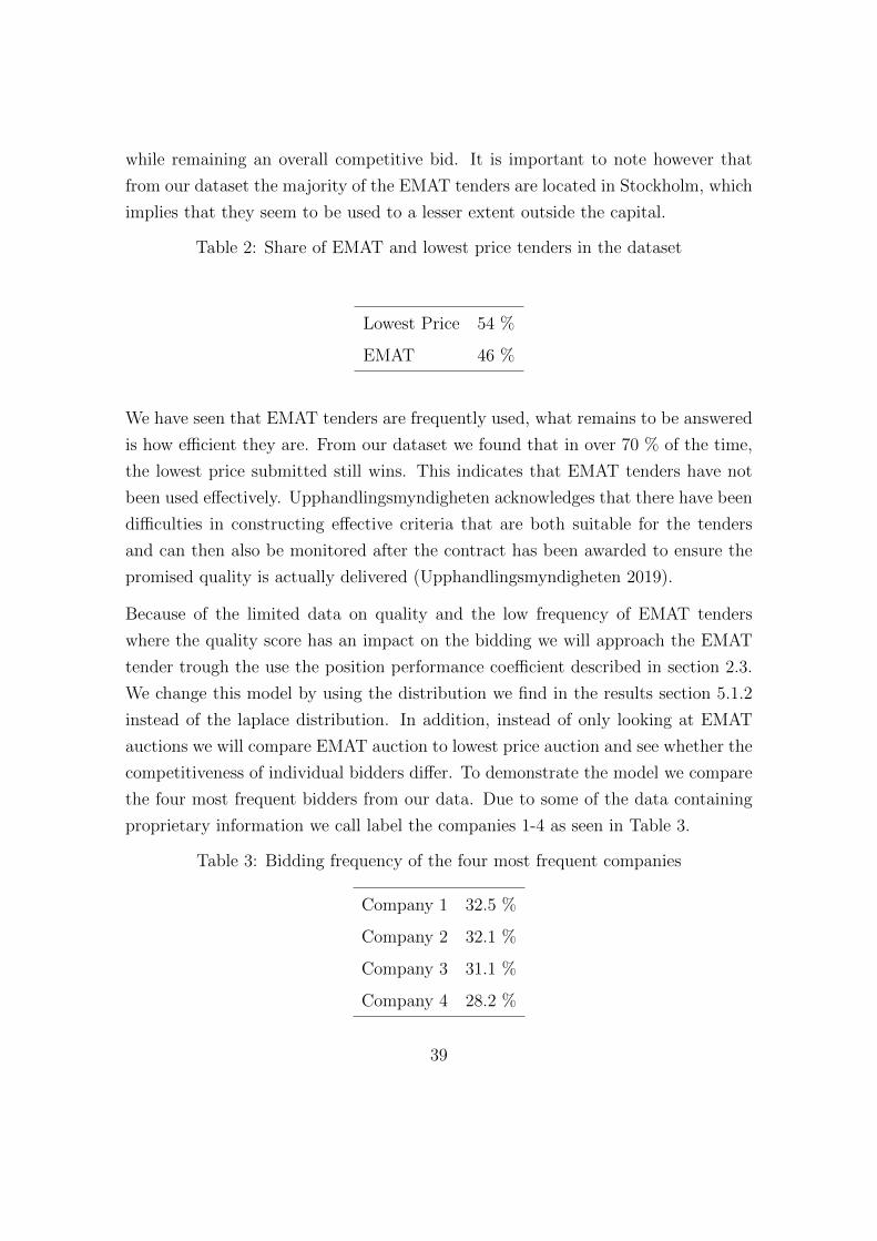
while remaining an overall competitive bid. It is important to note however that

from our dataset the majority of the EMAT tenders are located in Stockholm, which

implies that they seem to be used to a lesser extent outside the capital.

Table 2: Share of EMAT and lowest price tenders in the dataset

Lowest Price 54 %

EMAT 46 %

We have seen that EMAT tenders are frequently used, what remains to be answered

is how efficient they are. From our dataset we found that in over 70 % of the time,

the lowest price submitted still wins. This indicates that EMAT tenders have not

been used effectively. Upphandlingsmyndigheten acknowledges that there have been

difficulties in constructing effective criteria that are both suitable for the tenders

and can then also be monitored after the contract has been awarded to ensure the

promised quality is actually delivered (Upphandlingsmyndigheten 2019).

Because of the limited data on quality and the low frequency of EMAT tenders

where the quality score has an impact on the bidding we will approach the EMAT

tender trough the use the position performance coefficient described in section 2.3.

We change this model by using the distribution we find in the results section 5.1.2

instead of the laplace distribution. In addition, instead of only looking at EMAT

auctions we will compare EMAT auction to lowest price auction and see whether the

competitiveness of individual bidders differ. To demonstrate the model we compare

the four most frequent bidders from our data. Due to some of the data containing

proprietary information we call label the companies 1-4 as seen in Table 3.

Table 3: Bidding frequency of the four most frequent companies

Company 1 32.5 %

Company 2 32.1 %

Company 3 31.1 %

Company 4 28.2 %

39

5 Results

We present our results in the order they were presented in the Methodology section,

beginning with analyzing tender participation collectively and individually. Then

we look at price prediction for our two dependent variables and finally show how

one can assess performance in EMAT tenders.

5.1 Bid/no Bid Decision

Firstly we present the results for the bid/no bid Decision. We begin the section by

looking at what impact the number of bidders have on tender price. Thereafter we

fit a distribution function to the tender participation data. We finish the section

by studying what factors affect the decision to bid and we compare these to probit

regression looking at individual companies at a micro level.

5.1.1 Number of Bidder’s Effect on Price

Using the bid spread as a proxy for competitiveness as described in the methodol-

ogy section 4.3 our results are presented below. We find that the with a significant

and negative coefficient of -0.0110 that increasing the number of competitors de-

creases the competitiveness spread implying that more participants result in a more

competitive bidding process.

40

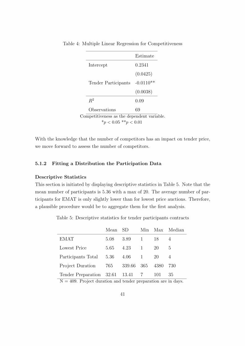
Table 4: Multiple Linear Regression for Competitiveness

Estimate

Intercept 0.2341

(0.0425)

Tender Participants -0.0110**

(0.0038)

R2 0.09

Observations 69

Competitiveness as the dependent variable.

*p < 0.05 **p < 0.01

With the knowledge that the number of competitors has an impact on tender price,

we move forward to assess the number of competitors.

5.1.2 Fitting a Distribution the Participation Data

Descriptive Statistics

This section is initiated by displaying descriptive statistics in Table 5. Note that the

mean number of participants is 5.36 with a max of 20. The average number of par-

ticipants for EMAT is only slightly lower than for lowest price auctions. Therefore,

a plausible procedure would be to aggregate them for the first analysis.

Table 5: Descriptive statistics for tender participants contracts

Mean SD Min Max Median

EMAT 5.08 3.89 1 18 4

Lowest Price 5.65 4.23 1 20 5

Participants Total 5.36 4.06 1 20 4

Project Duration 765 339.66 365 4380 730

Tender Preparation 32.61 13.41 7 101 35

N = 409. Project duration and tender preparation are in days.

41

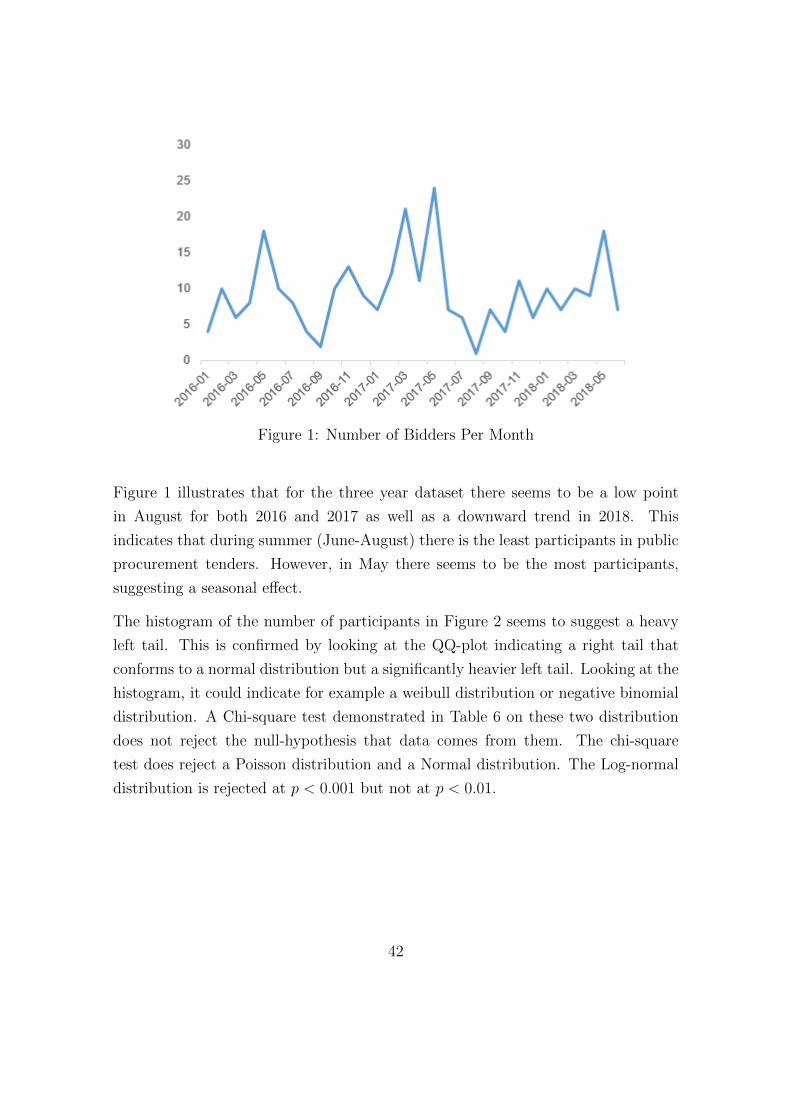
Figure 1: Number of Bidders Per Month

Figure 1 illustrates that for the three year dataset there seems to be a low point

in August for both 2016 and 2017 as well as a downward trend in 2018. This

indicates that during summer (June-August) there is the least participants in public

procurement tenders. However, in May there seems to be the most participants,

suggesting a seasonal effect.

The histogram of the number of participants in Figure 2 seems to suggest a heavy

left tail. This is confirmed by looking at the QQ-plot indicating a right tail that

conforms to a normal distribution but a significantly heavier left tail. Looking at the

histogram, it could indicate for example a weibull distribution or negative binomial

distribution. A Chi-square test demonstrated in Table 6 on these two distribution

does not reject the null-hypothesis that data comes from them. The chi-square

test does reject a Poisson distribution and a Normal distribution. The Log-normal

distribution is rejected at p < 0.001 but not at p < 0.01.

42

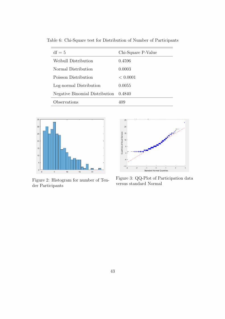
Table 6: Chi-Square test for Distribution of Number of Participants

df = 5 Chi-Square P-Value

Weibull Distribution 0.4596

Normal Distribution 0.0003

Poisson Distribution < 0.0001

Log-normal Distribution 0.0055

Negative Binomial Distribution 0.4840

Observations 409

Figure 2: Histogram for number of Ten-der Participants

Figure 3: QQ-Plot of Participation dataversus standard Normal

43

We proceed with testing fit by log-likelihood and AIC, the model that shows the best

fit is the Negative Binomial because it has the highest log-likelihood and smallest

AIC. The parameters we obtain with maximum likelihood estimation is: r = 3.390

and p = 0.3480 as illustrated in Figure 4. If we call number of participants a

stochastic variable P then P ∼ NB(3.390, 0.3480). This result will be used in

section 5.3.

Figure 4: Negative Binomial fitted to participation data

Table 7: Distribution model test for participants

Log-likelihood AIC

Negative Binomial -768.9 1542

Geometric -818.5 1639

Uniform -877.9 1758

Poisson -878.7 1759

Observations 409

44

5.1.3 Factors Contributing to Participants With Regression

As explained in the Methodology section 3.4, count data regression is normally better

fitted to a generalized linear regression model belonging to the Poisson regression

family. Below an OLS regression is compared to Poisson Regression, Truncated

Poisson Regression, Generalized Poisson and a Negative Binomial Regression Model.

Table 8 contains the results for the entire dataset for Stockholm County, Vastra

Gotaland County, Skane County and Ostergotland County. A notable results is

that the standard error for most of the coefficients in the OLS model seem to be

high in comparison to the estimate, thus indicating that the model has a bad fit

which further justifies our count data regression. At the end of this section we

demonstrate a diagnostic analysis of the standard OLS model to investigate among

other things the dependence between the explanatory variables.

45

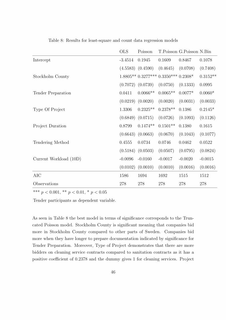
Table 8: Results for least-square and count data regression models

OLS Poisson T.Poisson G.Poisson N.Bin

Intercept -3.4514 0.1945 0.1609 0.8467 0.1078

(4.5583) (0.4590) (0.4645) (0.0708) (0.7408)

Stockholm County 1.8805** 0.3277*** 0.3350*** 0.2308* 0.3152**

(0.7072) (0.0739) (0.0750) (0.1333) 0.0995

Tender Preparation 0.0411 0.0066** 0.0065** 0.0077* 0.0060*

(0.0219) (0.0020) (0.0020) (0.0031) (0.0033)

Type Of Project 1.3306 0.2325** 0.2378** 0.1386 0.2145*

(0.6849) (0.0715) (0.0726) (0.1093) (0.1126)

Project Duration 0.8799 0.1474** 0.1501** 0.1380 0.1615

(0.6643) (0.0663) (0.0670) (0.1043) (0.1077)

Tendering Method 0.4555 0.0734 0.0746 0.0462 0.0522

(0.5184) (0.0503) (0.0507) (0.0795) (0.0824)

Current Workload (10D) -0.0096 -0.0160 -0.0017 -0.0020 -0.0015

(0.0102) (0.0010) (0.0010) (0.0016) (0.0016)

AIC 1586 1694 1692 1515 1512

Observations 278 278 278 278 278

*** p < 0.001, ** p < 0.01, * p < 0.05

Tender participants as dependent variable.

As seen in Table 8 the best model in terms of significance corresponds to the Trun-

cated Poisson model. Stockholm County is significant meaning that companies bid

more in Stockholm County compared to other parts of Sweden. Companies bid

more when they have longer to prepare documentation indicated by significance for

Tender Preparation. Moreover, Type of Project demonstrates that there are more

bidders on cleaning service contracts compared to sanitation contracts as it has a

positive coefficient of 0.2378 and the dummy gives 1 for cleaning services. Project

46

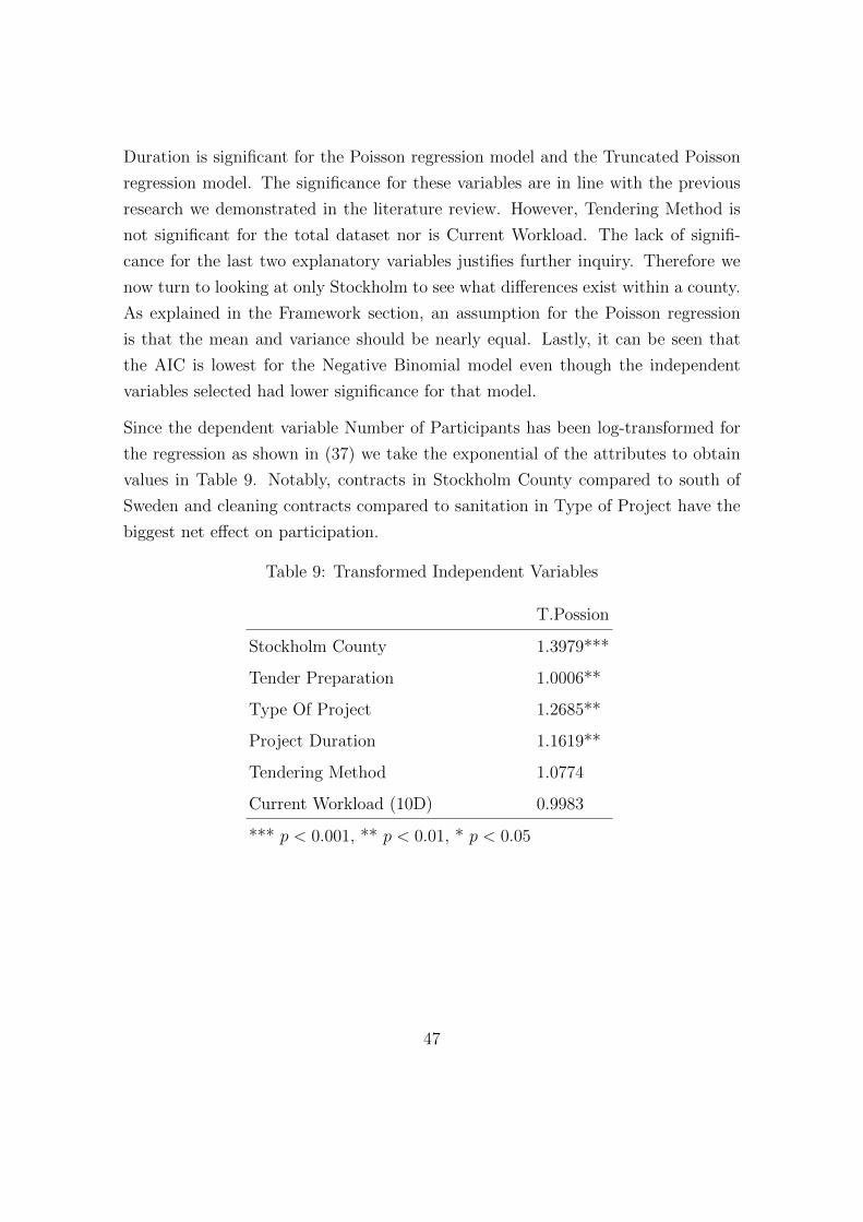
Duration is significant for the Poisson regression model and the Truncated Poisson

regression model. The significance for these variables are in line with the previous

research we demonstrated in the literature review. However, Tendering Method is

not significant for the total dataset nor is Current Workload. The lack of signifi-

cance for the last two explanatory variables justifies further inquiry. Therefore we

now turn to looking at only Stockholm to see what differences exist within a county.

As explained in the Framework section, an assumption for the Poisson regression

is that the mean and variance should be nearly equal. Lastly, it can be seen that

the AIC is lowest for the Negative Binomial model even though the independent

variables selected had lower significance for that model.

Since the dependent variable Number of Participants has been log-transformed for

the regression as shown in (37) we take the exponential of the attributes to obtain

values in Table 9. Notably, contracts in Stockholm County compared to south of

Sweden and cleaning contracts compared to sanitation in Type of Project have the

biggest net effect on participation.

Table 9: Transformed Independent Variables

T.Possion

Stockholm County 1.3979***

Tender Preparation 1.0006**

Type Of Project 1.2685**

Project Duration 1.1619**

Tendering Method 1.0774

Current Workload (10D) 0.9983

*** p < 0.001, ** p < 0.01, * p < 0.05

47

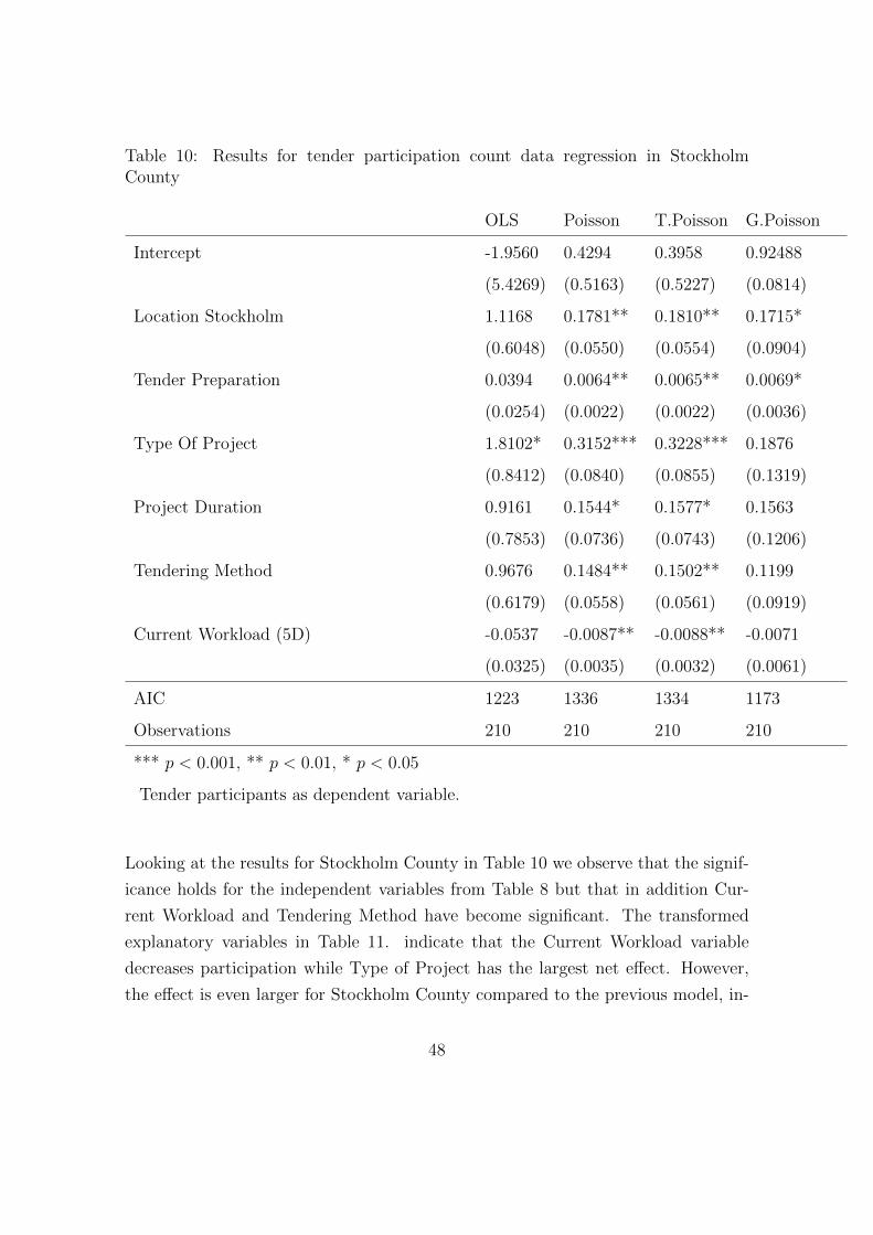
Table 10: Results for tender participation count data regression in StockholmCounty

OLS Poisson T.Poisson G.Poisson

Intercept -1.9560 0.4294 0.3958 0.92488

(5.4269) (0.5163) (0.5227) (0.0814)

Location Stockholm 1.1168 0.1781** 0.1810** 0.1715*

(0.6048) (0.0550) (0.0554) (0.0904)

Tender Preparation 0.0394 0.0064** 0.0065** 0.0069*

(0.0254) (0.0022) (0.0022) (0.0036)

Type Of Project 1.8102* 0.3152*** 0.3228*** 0.1876

(0.8412) (0.0840) (0.0855) (0.1319)

Project Duration 0.9161 0.1544* 0.1577* 0.1563

(0.7853) (0.0736) (0.0743) (0.1206)

Tendering Method 0.9676 0.1484** 0.1502** 0.1199

(0.6179) (0.0558) (0.0561) (0.0919)

Current Workload (5D) -0.0537 -0.0087** -0.0088** -0.0071

(0.0325) (0.0035) (0.0032) (0.0061)

AIC 1223 1336 1334 1173

Observations 210 210 210 210

*** p < 0.001, ** p < 0.01, * p < 0.05

Tender participants as dependent variable.

Looking at the results for Stockholm County in Table 10 we observe that the signif-

icance holds for the independent variables from Table 8 but that in addition Cur-

rent Workload and Tendering Method have become significant. The transformed

explanatory variables in Table 11. indicate that the Current Workload variable

decreases participation while Type of Project has the largest net effect. However,

the effect is even larger for Stockholm County compared to the previous model, in-

48

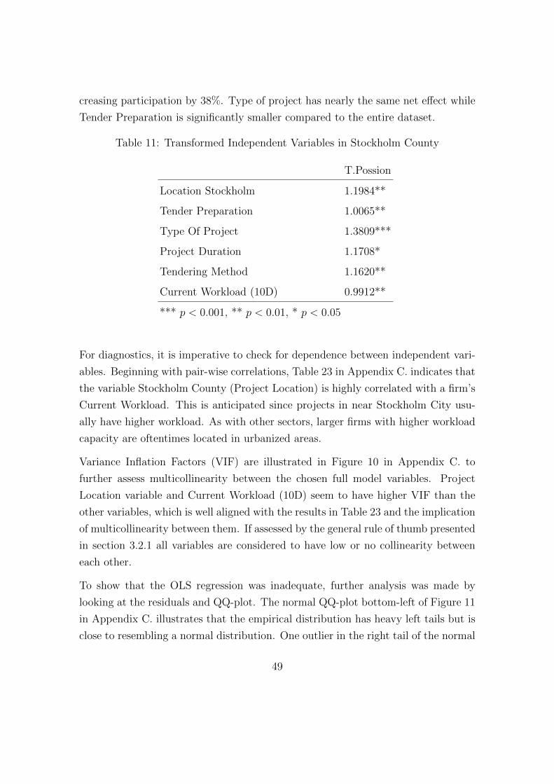
creasing participation by 38%. Type of project has nearly the same net effect while

Tender Preparation is significantly smaller compared to the entire dataset.

Table 11: Transformed Independent Variables in Stockholm County

T.Possion

Location Stockholm 1.1984**

Tender Preparation 1.0065**

Type Of Project 1.3809***

Project Duration 1.1708*

Tendering Method 1.1620**

Current Workload (10D) 0.9912**

*** p < 0.001, ** p < 0.01, * p < 0.05

For diagnostics, it is imperative to check for dependence between independent vari-

ables. Beginning with pair-wise correlations, Table 23 in Appendix C. indicates that

the variable Stockholm County (Project Location) is highly correlated with a firm’s

Current Workload. This is anticipated since projects in near Stockholm City usu-

ally have higher workload. As with other sectors, larger firms with higher workload

capacity are oftentimes located in urbanized areas.

Variance Inflation Factors (VIF) are illustrated in Figure 10 in Appendix C. to

further assess multicollinearity between the chosen full model variables. Project

Location variable and Current Workload (10D) seem to have higher VIF than the

other variables, which is well aligned with the results in Table 23 and the implication

of multicollinearity between them. If assessed by the general rule of thumb presented

in section 3.2.1 all variables are considered to have low or no collinearity between

each other.

To show that the OLS regression was inadequate, further analysis was made by

looking at the residuals and QQ-plot. The normal QQ-plot bottom-left of Figure 11

in Appendix C. illustrates that the empirical distribution has heavy left tails but is

close to resembling a normal distribution. One outlier in the right tail of the normal

49

QQ-plot was removed after testing multicollinearity. Furthermore, the residual plot

on top-left is well aligned with the results seen in the normal QQ-plot since the

left tail residuals deviates more than the remaining data from the majority of the

other fitted residuals. Inspecting the residual plot it is seen that the residuals does

indeed not follow a N(0, 1)-distribution, implying that they in fact are under impact

by heteroskedacity. The residuals coinciding with a normal distribution contradicts

the normality assumption for error terms in an OLS model. Variables was not

transformed to achieve homoskedacity since it could discard important information

in models that describes number of participants.

Finally, an all possible regression was performed based on the selection criteria

BIC. The model that described the number of competitors in a contract best was

whether it was located in Stockholm or another County in Sweden. Figure 12 in

Appendix C. illustrates that the multiple regression analysis might not be the best

suitable approach to model the number of participants in a contract. Omitted

variable bias has to be considered when computing a model that describe number

of participants in a contract. Surprisingly, the numbers of competitors increases the

closer Stockholm City the contract is based. The diagnostic results presented in this

section is well aligned with the results displayed in Table 10, which displays that

OLS does not perform well.

50

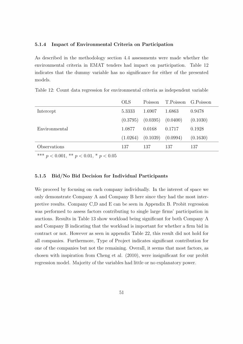
5.1.4 Impact of Environmental Criteria on Participation

As described in the methodology section 4.4 assessments were made whether the

environmental criteria in EMAT tenders had impact on participation. Table 12

indicates that the dummy variable has no significance for either of the presented

models.

Table 12: Count data regression for environmental criteria as independent variable

OLS Poisson T.Poisson G.Poisson

Intercept 5.3333 1.6907 1.6863 0.9478

(0.3795) (0.0395) (0.0400) (0.1030)

Environmental 1.0877 0.0168 0.1717 0.1928

(1.0264) (0.1039) (0.0994) (0.1630)

Observations 137 137 137 137

*** p < 0.001, ** p < 0.01, * p < 0.05

5.1.5 Bid/No Bid Decision for Individual Participants

We proceed by focusing on each company individually. In the interest of space we

only demonstrate Company A and Company B here since they had the most inter-

pretive results. Company C,D and E can be seen in Appendix B. Probit regression

was performed to assess factors contributing to single large firms’ participation in

auctions. Results in Table 13 show workload being significant for both Company A

and Company B indicating that the workload is important for whether a firm bid in

contract or not. However as seen in appendix Table 22, this result did not hold for

all companies. Furthermore, Type of Project indicates significant contribution for

one of the companies but not the remaining. Overall, it seems that most factors, as

chosen with inspiration from Cheng et al. (2010), were insignificant for our probit

regression model. Majority of the variables had little or no explanatory power.

51

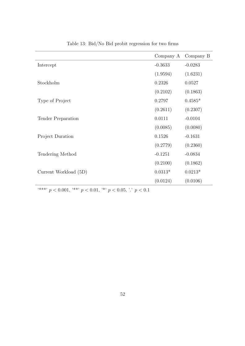
Table 13: Bid/No Bid probit regression for two firms

Company A Company B

Intercept -0.3633 -0.0283

(1.9594) (1.6231)

Stockholm 0.2326 0.0527

(0.2102) (0.1863)

Type of Project 0.2797 0.4585*

(0.2611) (0.2307)

Tender Preparation 0.0111 -0.0104

(0.0085) (0.0080)

Project Duration 0.1526 -0.1631

(0.2779) (0.2360)

Tendering Method -0.1251 -0.0834

(0.2100) (0.1862)

Current Workload (5D) 0.0313* 0.0213*

(0.0124) (0.0106)

’***’ p < 0.001, ’**’ p < 0.01, ’*’ p < 0.05, ’.’ p < 0.1

52

5.2 Predicting Price

This section intend to present the results on price performance. As explained in the

Methodology section we first look at floor care unit prices as the dependent variable

and then compare with the spread dependent variable.

5.2.1 Factors Affecting Pricing

We begin by testing a linear relationship between the unit prices and independent

variables with a multiple linear regression to examine what factors affect the pricing

decision. The independent variables included are demonstrated in section 4.5.1. The

results in Table 14 indicates that Tendering Method is significant with companies

placing lower bids for lowest price compared to EMAT tenders. The Location North

dummy is significant with a positive value of 0.4808 which implies that contracts

in the north receive higher bids. The dummy corresponding to small companies is

significant but at the lowest significance level, with a value of 0.2910 it could indicate

that smaller companies bid higher than larger ones. Because the significance is so

low we further explore the dynamic between large and small companies in sections

5.2.3 and 5.2.4.

53

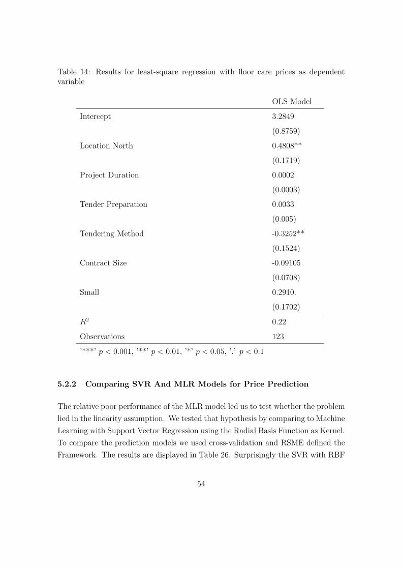
Table 14: Results for least-square regression with floor care prices as dependentvariable

OLS Model

Intercept 3.2849

(0.8759)

Location North 0.4808**

(0.1719)

Project Duration 0.0002

(0.0003)

Tender Preparation 0.0033

(0.005)

Tendering Method -0.3252**

(0.1524)

Contract Size -0.09105

(0.0708)

Small 0.2910.

(0.1702)

R2 0.22

Observations 123

’***’ p < 0.001, ’**’ p < 0.01, ’*’ p < 0.05, ’.’ p < 0.1

5.2.2 Comparing SVR And MLR Models for Price Prediction

The relative poor performance of the MLR model led us to test whether the problem

lied in the linearity assumption. We tested that hypothesis by comparing to Machine

Learning with Support Vector Regression using the Radial Basis Function as Kernel.

To compare the prediction models we used cross-validation and RSME defined the

Framework. The results are displayed in Table 26. Surprisingly the SVR with RBF

54

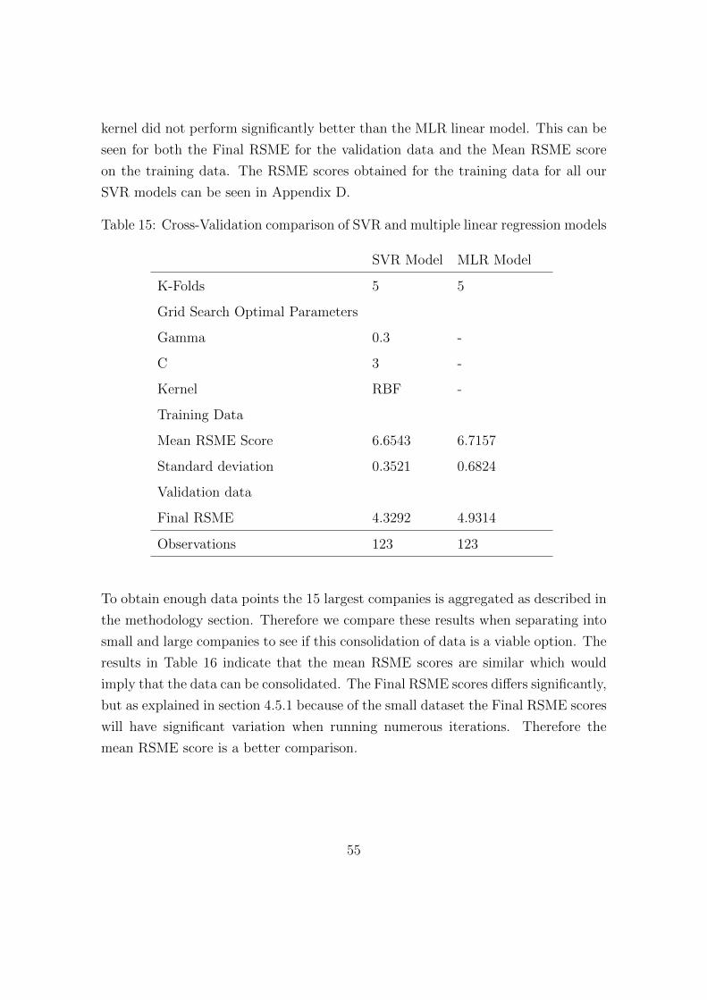
kernel did not perform significantly better than the MLR linear model. This can be

seen for both the Final RSME for the validation data and the Mean RSME score

on the training data. The RSME scores obtained for the training data for all our

SVR models can be seen in Appendix D.

Table 15: Cross-Validation comparison of SVR and multiple linear regression models

SVR Model MLR Model

K-Folds 5 5

Grid Search Optimal Parameters

Gamma 0.3 -

C 3 -

Kernel RBF -

Training Data

Mean RSME Score 6.6543 6.7157

Standard deviation 0.3521 0.6824

Validation data

Final RSME 4.3292 4.9314

Observations 123 123

To obtain enough data points the 15 largest companies is aggregated as described in

the methodology section. Therefore we compare these results when separating into

small and large companies to see if this consolidation of data is a viable option. The

results in Table 16 indicate that the mean RSME scores are similar which would

imply that the data can be consolidated. The Final RSME scores differs significantly,

but as explained in section 4.5.1 because of the small dataset the Final RSME scores

will have significant variation when running numerous iterations. Therefore the

mean RSME score is a better comparison.

55

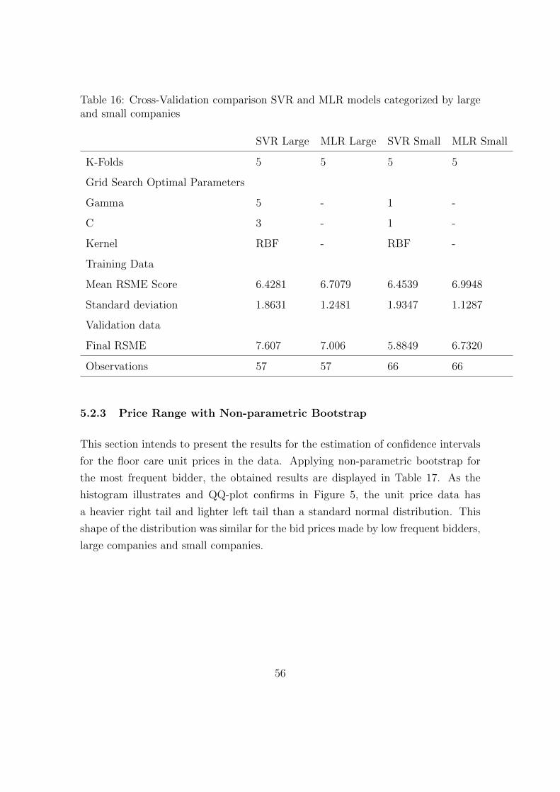
Table 16: Cross-Validation comparison SVR and MLR models categorized by largeand small companies

SVR Large MLR Large SVR Small MLR Small

K-Folds 5 5 5 5

Grid Search Optimal Parameters

Gamma 5 - 1 -

C 3 - 1 -

Kernel RBF - RBF -

Training Data

Mean RSME Score 6.4281 6.7079 6.4539 6.9948

Standard deviation 1.8631 1.2481 1.9347 1.1287

Validation data

Final RSME 7.607 7.006 5.8849 6.7320

Observations 57 57 66 66

5.2.3 Price Range with Non-parametric Bootstrap

This section intends to present the results for the estimation of confidence intervals

for the floor care unit prices in the data. Applying non-parametric bootstrap for

the most frequent bidder, the obtained results are displayed in Table 17. As the

histogram illustrates and QQ-plot confirms in Figure 5, the unit price data has

a heavier right tail and lighter left tail than a standard normal distribution. This

shape of the distribution was similar for the bid prices made by low frequent bidders,

large companies and small companies.

56

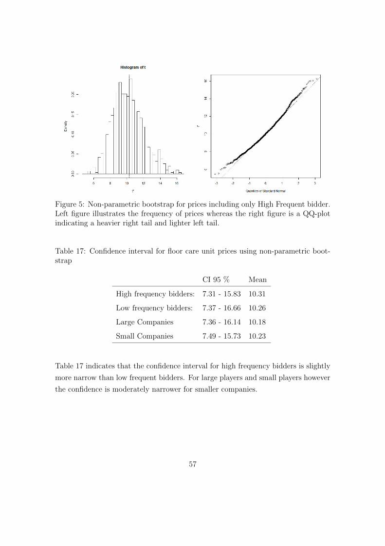
Figure 5: Non-parametric bootstrap for prices including only High Frequent bidder.Left figure illustrates the frequency of prices whereas the right figure is a QQ-plotindicating a heavier right tail and lighter left tail.

Table 17: Confidence interval for floor care unit prices using non-parametric boot-strap

CI 95 % Mean

High frequency bidders: 7.31 - 15.83 10.31

Low frequency bidders: 7.37 - 16.66 10.26

Large Companies 7.36 - 16.14 10.18

Small Companies 7.49 - 15.73 10.23

Table 17 indicates that the confidence interval for high frequency bidders is slightly

more narrow than low frequent bidders. For large players and small players however

the confidence is moderately narrower for smaller companies.

57

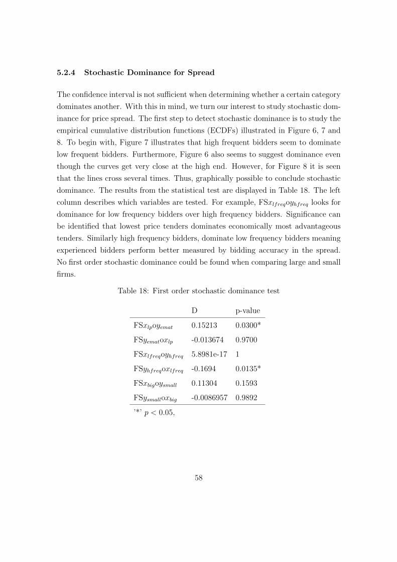
5.2.4 Stochastic Dominance for Spread

The confidence interval is not sufficient when determining whether a certain category

dominates another. With this in mind, we turn our interest to study stochastic dom-

inance for price spread. The first step to detect stochastic dominance is to study the

empirical cumulative distribution functions (ECDFs) illustrated in Figure 6, 7 and

8. To begin with, Figure 7 illustrates that high frequent bidders seem to dominate

low frequent bidders. Furthermore, Figure 6 also seems to suggest dominance even

though the curves get very close at the high end. However, for Figure 8 it is seen

that the lines cross several times. Thus, graphically possible to conclude stochastic

dominance. The results from the statistical test are displayed in Table 18. The left

column describes which variables are tested. For example, FSxlfreqoyhfreq looks for

dominance for low frequency bidders over high frequency bidders. Significance can

be identified that lowest price tenders dominates economically most advantageous

tenders. Similarly high frequency bidders, dominate low frequency bidders meaning

experienced bidders perform better measured by bidding accuracy in the spread.

No first order stochastic dominance could be found when comparing large and small

firms.

Table 18: First order stochastic dominance test

D p-value

FSxlpoyemat 0.15213 0.0300*

FSyematoxlp -0.013674 0.9700

FSxlfreqoyhfreq 5.8981e-17 1

FSyhfreqoxlfreq -0.1694 0.0135*

FSxbigoysmall 0.11304 0.1593

FSysmalloxbig -0.0086957 0.9892

’*’ p < 0.05,

58

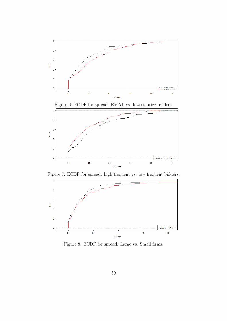
Figure 6: ECDF for spread. EMAT vs. lowest price tenders.

Figure 7: ECDF for spread. high frequent vs. low frequent bidders.

Figure 8: ECDF for spread. Large vs. Small firms.

59

5.2.5 Price Performance with Spread Variable

The procedures in section 5.2.2 are repeated for the support vector regression and

multiple linear regression by changing the dependent variable from unit prices to

the spread defined in section 4.2. Same pattern can be read that the MLR performs

equally to the SVR. However, the spread variable performs worse in prediction

compared to the unit prices.

Table 19: Cross-Validation Comparison SVR and MLR Models with spread as priceperformance indicator

SVR Big MLR Big SVR Small MLR Small

K-Folds 5 5 5 5

Grid Search Optimal Parameters

Gamma 1 - 0.3 -

C 10 - 1 -

kernel RBF - RBF -

Training Data

Mean RSME Scores 0.3796 0.3797 0.4238 0.4483

Standard deviation 0.0898 0.1664 0.1663 0.1289

Validation data

Final RSME 0.3474 0.3716 0.2169 0.2632

Observations 150 150 135 135

60

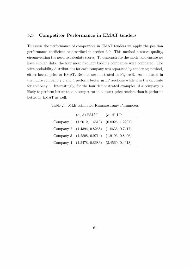
5.3 Competitor Performance in EMAT tenders

To assess the performance of competitors in EMAT tenders we apply the position

performance coefficient as described in section 3.9. This method assesses quality,

circumventing the need to calculate scores. To demonstrate the model and ensure we

have enough data, the four most frequent bidding companies were compared. The

joint probability distributions for each company was separated by tendering method,

either lowest price or EMAT. Results are illustrated in Figure 9. As indicated in

the figure company 2,3 and 4 perform better in LP auctions while it is the opposite

for company 1. Interestingly, for the four demonstrated examples, if a company is

likely to perform better than a competitor in a lowest price tenders than it performs

better in EMAT as well.

Table 20: MLE estimated Kumaraswamy Parameters

(α, β) EMAT (α, β) LP

Company 1 (1.2012, 1.4510) (0.8025, 1.2207)

Company 2 (1.4394, 0.8268) (1.8635, 0.7417)

Company 3 (1.2808, 0.9714) (1.9193, 0.8406)

Company 4 (1.5478, 0.8683) (3.4560, 0.4918)

61

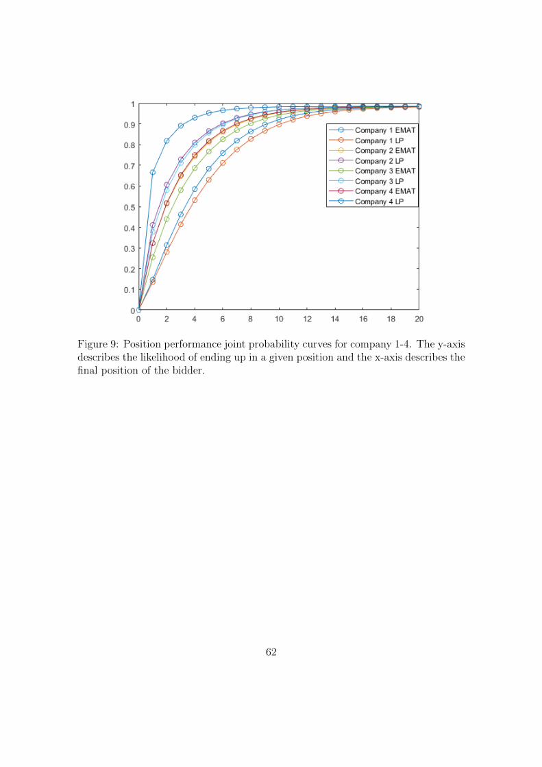
Figure 9: Position performance joint probability curves for company 1-4. The y-axisdescribes the likelihood of ending up in a given position and the x-axis describes thefinal position of the bidder.

62

6 Analysis of Results

Our results have given us some important takeaways. To begin with we found

that the number of bidders have an impact on tender price. This result led us

to conclude that number of competitors must be accounted for in a bidding model.

Our tender participation regression found several significant variables while for price

prediction we surprisingly found equal performance of multiple linear regression

models compared to more advanced support vector regression with RBF kernel.

We found that experienced bidders perform better in bidding, companies bid more

evenly in lowest price than in EMAT tenders but did not find enough evidence that

larger companies perform better than smaller ones. Below we go into more detail of

the results.

6.1 Number of Competitors

As expected the Poisson and Truncated Poisson model performed better than the

MLR model on the count data. The Generalized Poisson did not perform well when

describing the number of competitors in a tender in comparison to Poisson and

Truncated Poisson. Results from the Generalized Poisson model did not exhibit any

notable statistical significant variables except for the dummy Stockholm County and

Tender Preparation. The negative Binomial model gave the best model fit by the

selective criteria, which is in line with Lundberg et al. (2015) that used only this

regression for a study in the cleaning sector. The negative binomial model should

perform well when the equidispersion assumption does not hold, that is when the

mean value does not equal the variance. And as our descriptive statistics indicate,

the assumption does not hold for our data. Thus, the negative binomial ought to

perform better. Which it does measured by the AIC, but it has lower significance for

the explanatory variables. Thus, even though the truncated Poisson is chosen as our

model because it explained the independent variables the best, the negative binomial

had the lowest AIC which is a drawback for our model. The negative binomial still

shows significance for Stockholm County, Tender Preparation and Type of Project

albeit at a lower significance level so these are the significance results we can be

63

most confident in. The fact that project duration loses significance for the Negative

Binomial is not surprising. When looking through the raw data, the project duration

in the cleaning contracts is almost exclusively less than three years with the majority

of the project within two years. Compare this to the results obtained by (Vigren

2017) where project duration was significant for bus transport. Those contracts

ranged up to 7-8 years. So naturally in that instance the bidder is more likely to

take duration into account. The pattern was the same for the Stockholm County

data with the negative binomial lowering the significance for most variables. It is

not surprising that the Truncated Poisson model performed better than the regular

Poisson since the latter does not take zeros into account in the dependent variable.

Lastly, as our diagnostic for the MLR participant model indicated, the standard

assumptions of homoscedasticity in the OLS regression were not fulfilled, implying

that such as model could be discarded when assessing public procurement within

the cleaning sector.

Comparing our count data regression models for mainly Stockholm County with the

full dataset including all counties, Tendering Method and Current Workload became

significant. We expected Current Workload to become significant looking at a spe-

cific counties considering how firms make resource allocation decisions in cleaning.

The main asset of cleaning services companies is the labour force. Therefore, we do

not expect that a firm is willing to move their labour force far distances and thus

any choice regarding distribution of resources will not be on a cross-county line but

rather within each county. Moreover, many of the companies in our dataset act

locally. However, it it more surprising that Tendering Method became significant,

indicating that companies in Stockholm participate more on lowest price tenders

compared to EMAT tenders. This could be interpreted as larger participants in

Stockholm County deeming EMAT contracts to be unreliable. Our review of the

raw data for EMAT tenders indicated that larger participants in EMAT contracts

usually achieve the same scores thus making the EMAT grading system obsolete

since other companies can place sham offerings and still win the contracts. The

incentives for participants to commit to EMAT contracts are thus lower than for

lowest price contracts. Nevertheless, the difference in results for Tendering Method

between the two models may simply be due to the fact that so many of the con-

64

tracts outside Stockholm are just lowest price, contributing to uncertainty in the

significance results.

Tender Preparation was significant for both models and at equal value, implying that

the preparation of documents is an important aspect all around for several counties.

These results are in line with previous research where Tender Preparation has been

featured prominently, both with regard to the participation and pricing decision.

Another interesting, albeit expected, outcome for Stockholm County is that Location

Stockholm gives significance, showing that companies are more inclined to bid on

contracts that are in Stockholm city compared to the rest of the county. This is

not unanticipated since contracts in large cities tend to be more attractive from a

financial perspective. It is reasonable to assume that the bid prices in comparison

to firm costs are higher in large cities than for projects taken in the outskirts.

The Type of Project variable had a big net effect in both datasets, indicating that

regular cleaning contracts to a larger degree increase the number of bidding partic-

ipants compared to sanitation contracts.

Lastly, we used the count data regression models to see if the inclusion of environ-

mental criteria has any affect on participation. The results showed there was no

significance. This could either be because most companies fulfill the environmental

criteria which entail providing certificates. Equally, it could also mean that partici-

pants do not consider the criteria effective. Meaning that there is not enough gover-

nance regarding living up to what has been stipulated in the contract. So they can

commit to fulfilling demands, knowing it is difficult to control they are upholding the

promises. This would be in line with the concerns from Upphandlingsmyndigheten

that we mentioned in section 2.4, that there is an underlying problem in selecting

good criteria that can be efficiently measured and governed.

65

6.2 Bid/No Bid Logistic Regression

Many of the variables that were significant before, become less significant or fully

disappeared when assessing the bid/no bid decision model at an individual level. We

did find some noteworthy results. For example the likelihood of bidding depended

on project location in Stockholm for small companies we looked at but not for larger

ones. For some companies the time allocated to prepare documents had an impact

on the decision. Surprisingly the current workload had significance with a positive

coefficient for one of our companies. That runs contrary to the results from the

Poisson regression and it reveals that current workload is a bad variable to include

in the individual bid/no bid decision. Naturally when there are several contracts,

the odds are that the company in question participated in at least one of them, and

so therefore it shows up as 1 in our data. The current workload measures whether

the overall participation goes down while the probit does not measure volume. We

conclude that current workload should not be included as a variable in the individual

model.

Overall, we conclude that the poor performance of all probit models seem to sug-

gest that looking at individual companies with the probit model will not render

good results and so the bid/no bid decision should be analyzed through aggregated

measures as in the Poisson regression or through another mathematical model.

6.3 Predicting Price

The first analysis we performed was a multiple linear regression on floor care unit

prices. With our given attributes our model fit was poor. Our initial hypothesis was

that the problem lay in the linearity assumption. Therefore, comparing the MLR

model to SVR it was surprising that the former performed comparably to the more

advanced machine learning model. This means we can not reject the idea that the

relationship is linear. It is then plausible to believe that the reason the prediction

is so poor is due to omitted variable bias, as previous studies showed, the unit

prices can suffer from high dimensionality. Previous research in construction found

more than 50 variables that affect the pricing decision of a bidder. Meaning there

66

are numerous attributes that have an impact which is likely the case for cleaning

services as well. The poor model fit for the unit price regression could also be

because the bidding behavior is random. The latter was one of the questions we

sought to answer with this thesis.

What speaks against the randomness argument is that we found significance for

Tendering Method, Location North and Company Size in the regression analysis,

albeit the latter at the lowest significance level. The Tendering Method dummy

indicates that companies bid lower in lowest price tenders compared to EMAT. This

is likely due to the fact that they are hoping that the points awarded in EMAT

tenders will be able to compensate for a higher price. The location dummy being

significant shows that companies bid lower in the south of Stockholm. This might

be due to the behavior of certain companies that primarily act in that region. On

the other hand, it could imply that contracts in the north are more expensive. The

latter is more likely as most large players bid all over Stockholm. The dummy

variable ’Small’ implies that large companies bid lower than smaller ones. The

result that small companies frequently bid higher can be due to the fact that large

companies have economies of scale. However, considering how standardized the

cleaning industry is it is more likely due to the experience that some large companies

have in addition to them having a designated bid manager, which likely bring with

it structure. Because the significance for company size was so weak we wanted to

further explore it with stochastic dominance and non-parametric bootstrapping. We

analyze these results in the next section.

Surprisingly for the unit price regression, contract size had no significance on the

pricing decision. The Contract Size variable was prominent in previous literature for

the construction sector but did not translate to the cleaning services. This could be

explained by the fact that the the Swedish cleaning industry does not bind the same

amount of capital as say the construction industry. Firms tend to approach contracts

with more caution the higher capital they have to tie up to certain projects. In the

cleaning industry, a majority of the tied up capital is the labour force, whereas in

the construction industry there are machinery, subcontractors and labour force to

mention a few.

67

For unit price prediction, to gather enough data for our test we wanted to see if

we could consolidate the data for the 15 largest companies for prediction. This

is a relevant this as we foresee that larger datasets of unit prices will take years

to obtain. Therefore one must have an alternative during this time. So we did

an additional test separating the data noting that it implied two small sample sizes

which will affect the results. Nonetheless, the mean scores did not differ significantly

which could indicate that you can consolidate the data while the final RSME sore

did differ but as explained it is not a trustworthy measure with less than 70 points

because it shows high variation as the sub-sample that ends up as validation data in

the k-fold method will be very different for such a small sample size. As we will see

in the next section, the differences in pricing seem to stem from experience rather

than size which would lend credibility to the possibility of consolidating data for

large players with similar experience.

Regarding differences between the two dependent variables we chose, our results

indicate that spread is not suitable as a dependent variable because the prediction

performed much worse compared to unit prices for both of our models. So our

approach of using the spread to obtain more data points is not a good way to

predict price performance with regression.

6.3.1 Stochastic Dominance and Non-Parametric Bootstrap Analysis

As explained above we wanted to further test the price performance. In particular

to differences between large and small players. From the bootstrapping we obtained

unit price confidence intervals for the categories described in section 4.5.2. Here the

interval was equal for large and small players but was narrower for more frequent

bidders compared to less frequent bidders. Due to data constraints we only used the

spread variable for stochastic dominance test. The results showed that both lowest

price tenders dominated EMAT and high frequent bidders dominated lower frequent

bidders at first order, i.e experience has an effect on performance. These results were

expected. However, it was surprising that large companies did not dominate smaller

ones at first order. This lends credibility to the theory we proposed above that

experience is more important than size in how bidders perform. Because the costs

68

are standardized it is less likely that economies of scale drive differences in pricing

rather than experience. However, as explained in section 4.5.2, to ensure enough

data for comparison we defined smaller companies as those with less than 125 MSEK

in revenue. Thus there are by no means small companies and perhaps significance

would have been found if we could compare to truly small companies such as those

with less than 10 MSEK. However, these tend to bid more sporadically and as a

result it is difficult to obtain sufficient data.

6.4 Quantifying Quality

Our initial goal was to predict the quality scores of each company just as with price.

It quickly became evident that this was not possible due to two reasons: Firstly,

because using EMAT criteria is not mandatory as we described in section 2.4 there

does not seem to be any standardized models for EMAT tenders; the procurement

entities use widely different criteria. This means that for each company there are

only 2-3 observations for the score they received per criteria in our dataset. Secondly

the larger companies tend to be awarded max points anyway. This results in the

lowest price bidder winning oftentimes. In fact, as we demonstrated in section 4.6

this tends to happen in more than 70 % of the cases. We therefore do not believe it

is feasible to assess the quality criteria even if we had data for an additional three

years.

Naturally, there are some instances where the quality score did impact outcome. And

as we found in section 5.2.1 companies tend to bid lower in EMAT tenders, expecting

their quality score to still keep them competitive. So we should still take this into

account. Our solution was to compare LP and EMAT tenders to see differences in

performance and see which ones are likely to be most competitive going forward.

Out of our sample of the four most frequent bidders the performance was consistent.

Meaning the company that was likely to be placed highest in lowest price tenders

was also likely to perform well in EMAT tenders. Using these results one can know

how competitive different competitors will be in an upcoming EMAT tender. So

for example if a hypothetical company G knows of a competitor that is expected

to participate and the model shows they have a high likelihood of placing badly in

69

EMAT tenders and Company G has a high likelihood of placing well then Company

G can expect to place a slightly higher bid while still being competitive. Clearly,

for this model to work perfectly we require a better prediction of each company’s

participation, and as explained in section 6.2 the probit models were inadequate for

explaining each company’s participation.

70

7 Conclusions

In this thesis we sought to understand what factors affected the decision making

of bidders in public procurement auction in the cleaning sector. For the bid/no

bid we found several factors that had an impact which were aligned with previous

research from construction. However, one major departure in our results was the low

significance of contract size on the pricing decision. We also found that in order to

make a good bid forecasting model one must predict both the price and the number

of competitors. For the impact of quality criteria we found that some companies

perform better in EMAT tenders compared to lowest price auctions and applied a

model that can be used to assess the performance of companies in EMAT tenders.

For tender participation it is imperative to use count data regression since ordinary

least-square regression perform poorly.

With regard to price prediction, we started this thesis declaring that our goal was

to examine whether prediction models for this sector was possible and in that case

what models were most suitable, or if the bidding behaviour is random. For the

first question our results were inconclusive. We had a good number of attributes

and the fact that they had such a low predictive power for both of our models

could indicate that there is some randomness in the bidding process. However, our

stochastic dominance test found that more experienced bidders perform better and

our non-parametric bootstrap showed that experienced bidders had a narrow bid

range which could mean there is more consistency in their bidding. So perhaps

the prediction models would improve if the data only consisted of the most frequent

bidders. But for that to work one must have access to a much bigger dataset. So since

we did find some differences between bidders we believe that rather than randomness

explaining the poor predictive performance it is the need for more attributes. One

might conclude that the low predictive power came from the small dataset but

since SVR is normally well equipped for small datasets we argue it is more likely

that what is required is more attributes. The models would presumably improve

with more granular data including factors such as type of floor, number of rooms

and area. However, a problem with this is of course that data like this is not

widely available in a structured way. During the work with this thesis we had the

71

opportunity to study these contracts in detail and it is clear that the sector suffers

from a lack of digitization and standards for submitting bids that companies adhere

to. Subsequently, key information such as the total area of the object is not available

and in cases that it is reported one must collect it individually from each contract.

This is not realistic for thousands of contracts. An essential attribute is the type

of floor that is cleaned. That information is often not available and we found that

prices could be several hundred percent higher for wood floor compared to plastic

floors. So naturally that is an attribute that is of utmost importance for a regression

analysis. Therefore, the key aspect to determine whether prediction is possible in

future studies will be to have access to more granular data

Surprisingly, the support vector regression with RBF kernel did not perform better

than multiple linear regression for both dependent variables. So the more advanced

machine learning models are not always better. Finally, one can draw the conclusion

that unit prices are a better approach for price prediction than the spread.

72

8 Suggestions for Future Research

As we concluded with regards to the SVR model it is quite adequate even with

smaller datasets so the problem of poor model fit is more likely due to missing

attributes. Therefore, with time as more companies become better at reporting their

data, more structurally good prediction models can be made. To exhaustively test

whether artificial intelligence could perform better than multiple linear regression,

other methods such as artificial neural networks should be tested although these are

generally more suitable for larger datasets.

A complete bid forecasting model requires knowledge of participation of individual

bidders. Our results with probit regression gave insufficient results, therefore one

should explore whether the prediction of individual participants is possible with

other models.

A final suggestion is to proceed by comparing the results we have obtained in the

cleaning industry and previous results from the construction on other areas of public

procurement to see if there are signifiant differences between industries in public

procurement.

73

Bibliography

Agerberg, J. and Agren, J. 2012. “Risk Management in the Tendering Process: A

survey of risk management practices within infrastructural construction.” Chalmers

University of Technology. Department of Technology Management and Economics.

Aldenius, M. and Khan, J. 2017. “Strategic use of green public procurement in the

bus sector: Challenges and opportunities.” Journal of Cleaner Production 164:250–

257.

Al-Arjani, A.H. 2002. “Type and size of project influences on number of bidders

for maintenance and operation projects in Saudi Arabia.” International Journal of

Project Management, 20(4):279–287.

Athey, S., Levin, J., and Seira, E. 2011. “Comparing open and sealed bid auctions:

Evidence from timber auctions,” The Quarterly Journal of Economics 126(1):207–

257.

Augustin, K. and Walter, M. 2010. “Operator changes through competitive tender-

ing: Empirical evidence from German local bus transport.” Research in Transporta-

tion Economics, 29(1):36–44.

Aurelien, G. 2017. Hands-On Machine Learning with Scikit-Learn and Tensorflow:

Concepts, Tools, and Techniques to Build Intelligent Systems. O’reilly Media.

Azman, M.A. 2014. “Number of Bidders in Small and Medium Public Construction

Procurement in Malaysia.” Applied Mechanics and Materials 567:595–600.

Bageis, A.S. and Fortune, C. 2009. “Factors affecting the bid/no bid decision in

the Saudi Arabian construction contractors.” Journal of Financial Management of

Property and Construction, 15(2):118–142.

Ballesteros-Perez, P., Campo-Hitscfeld, M., Mora-Melia, and Domınguez, D. 2015.

“Modeling Bidding Competitiveness and Position Performance in Multi-attribute

Construction Auctions.” Operations Research Perspectives, 2:24–35.

74

Ballesteros-Perez, P. and Skitmore, M. 2017. “On the Distribution of bids for Con-

struction Contract Auctions.” Construction Management and Economics, 35(3):106–

121.

Ballesteros-Perez, P., Skitmore, M., Pellicer, E., and Gutierrez-Bahamondes, J. 2016.

“Improving the Estimation of Probability of Bidder Participation in Procurement

Auctions.” International Journal of Project Management, 34(2):158–172.

Beck, A. 2011. “Experiences with competitive tendering of bus services in Germany.”

Transport Reviews, 31(3):313–339.

Benjamin, N.B.H. 1969. “Competitive bidding for building construction contracts.”

Stanford University. PhD dissertation.

Brook, M. 2016. Estimating and Tendering for Construction Work. Routledge 5th

ed.

Cameron, A.C. and Trivedo, P.K. 2005. Microeconometrics: Methods and Applica-

tions. Cambridge University Press.

Cheng, M-Y, Hsiang, C-C, Tsai, H-C, and Do, H-L. 2010. “Bidding Decision Making

for Construction Company Using a Multi-criteria Prospect Model.” Journal of Civil

Engineering and Management, 17(3):424–436.

Dikmen, I., Birgonul, M., and Kemal Gur, A. 2007. “A case-based Decision Support

Tool for Bid Mark-up Estimation of International Construction Projects.” Automa-

tion in Construction, 17(1):30–44.

Drew, D.S., Lo, Hing Po, and Skitmore, R.M. 2001. “The effect of client and type

and size of construction work on a contractor’s bidding strategy.” Elsevier, Building

and Environment 36(3):393–406.

Drew, D.S. and Skitmore, R.M. 2006. “Competitiveness in bidding: a consultant’s

perspective.” Construction Management and Economics, 10(3):227–247.

European Commission. 2017. “Public Procurement.” http://ec.europa.eu/trad

e/policy/accessing-markets/public-procurement/.

75

Fastighetsfolket. 2017. “Fler seriosa foretag avstar offentlig upphandling.” https:

//fastighetsfolket.se/2017/11/27/fler-seriosa-foretag-avstar-offentl

ig-upphandling/.

Fayek, A. 1998. “Competitive Bidding Strategy Model and Software System for Bid

Preparation.” Journal of Construction Engineering and Management, 124(1).

Friedman, L. 1956. “A Competitive-Bidding Strategy.” Operations Research, 4(1):104–

112.

Fu, W.K. 2003. “The Effect of Experience in Construction Contract Bidding.” De-

partment of Building and Real Estate. The Hong Kong Polytechnic University. De-

gree of Doctor of Philosophy at The Hong Kong Polytechnic University.

Hegazy, T. and Moselhi, O. 1994. “Analogy-based Solution to Markup Estimation

Problem.” Journal of Computing in Civil Engineering, 8(1):72–87.

Hestmati, A. and Maasoumi, E. 2000. “Stochastic Dominance Amongst Swedish

Income Distributions.” Econometric Reviews 19(3):287–320.

Hilbe, J. 2014. Modelling Count Data. Cambridge Books.

Hilbe, J.M. 2011. Negative Binomial Regression. New York: Cambridge Press 2nd

ed.

Hult, H., Lindskog, F., Hammarlind, O., and Rehn, CJ. 2012. Risk and Portfolio

Analysis: Principles and Methods. Springer-Verlag New York Inc. Springer Series in

Operations Research / Financial Engineering.

Inkopsradet. 2016. “Problemen med viktade utvarderingar.” Inkoprsradet. https:

//inkopsradet.se/expert/problemen-med-viktade-utvarderingar/.

James, G., Witten, D., Hastie, T., and Tibshirani, R. 2013. An Introduction to

Statistical Learning. Springer-Verlag New York Inc 1st ed.

Jung, H. and Kim, J-M. 2019. “Predicting Bid Prices by Using Machine Learning

Methods.” Applied Economics, 51(19):2011–2018.

76

Kleijnen, J. P.C and Schaik, F. D.J van. 2011. “Sealed-bid auction of Nether-

lands mussels: Statistical analysis.” International Journal of Production Economics,

132(1):154–161.

Li, H.. 1996. “Neural Network Models for Intelligent Support of Mark-up Estima-

tion.” Engineering Management, 131(4):391–399.

Lundberg, S., Marklund, P-O., and Brannlund, R. 2009. “Miljohansyn i offentlig

upphandling.” Konkurrensverket.

Lundberg, S., Marklund, P-O., and Stromback, E. 2016. “Is environmental policy

by public procurement effective?” Public Finance Review, 44(4):478–499.

Lundberg, S., Marklund, P-O, Stromback, E., and Sundstrom, D. 2015. “Using pub-

lic procurement to implement environment policy: an empirical analysis.” Umea

University Environmental Economics and Policy Studies, 17(4):487–520.

Malara, M. and Mazurkiewcz, M. 2012. “Modelling the Determinants of Winning

in Public Tendering Procedures Based on the Activity of a Selected Company.”

Operations and Research and Decisions, 22(1):51–62.

Montgomery, D. C., Peack, E. A., and Vining, G. G. 2012. Introduction to Linear

Regression Analysis. Wiley.

Petrovski, A., Petruseva, S., and Zileska, V. P. 2015. “Multiple Linear Regression

Model for Predicting Bidding Price.” Technics Technologies Education Management,

10(3):386–393.

Pla, A., Lopez, B., Murillo, J., and Maudet, N. 2014. “Multi-attribute Auctions With

Different Types of Attributes: Enacting Properties in Multi-attribute Auctions.”

Expert Systems with Applications, 41(10):4829–4843.

Polat, G., Bingol, B., Gurgun, A., and Yel, B. 2016. “Comparison of ANN and

MRA Approaches to Estimate Bid Mark-up Size in Public Construction Projects.”

Elsevier. Procedia Engineering, 164:331–338.

Regeringskansliet. 2019. “Regeringen kraftsamlar kring artificiell intelligens och oppna

data.” Regeringskansliet.

77

Renda, A., Pelkmans, J., Egenhofer, C., Schrefler, L., Luchetta, G., and Selcuki, C.

2012. “The Uptake of Green Public Procurement in the EU27.” European Comission,

DG Environment.

Schmid, F. and Trede, M. 1996. “Testing for First-Order Stochastic Dominance: A

New Distribution-Free Test. A New Distribution-Free Test.” Journal of the Royal

Statistical Society. Series D (The Statistician), 45(3):371–380.

Takano, Y., Ishii, N., Yu, W., and Muraki, M. 2018. “Determining Bid Markup and

Resources Allocated to Cost Estimation in Competitive Bidding.” Automation in

Construction, 85:358–368.

Testa, F., Annunziata, E., Iraldo, F., and Frey, M. 2013. “Drawbacks and oppor-

tunities of green public procurement: an effective tool for sustainable production.”

Journal of Cleaner Production, 112(3):1893–1900.

Thode, H. C. 2002. Testing for Normality. New York: Marcel Dekker 1st ed.

Upphandlingsmyndigheten. 2019. “Statistik om Offentlig Upphandling 2018.” Up-

phandlingsmyndighetens rapport 2018:2.

Vapnik, V. and Chapelle, O. 1999. “Model selection for support vector machines.”

MIT Press Cambridge 132:230–236.

Vigren, A. 2017. “How Many Want to Drive the Bus? Analyzing the Number of

Bids for Public Transport Bus Contracts.” Elsevier. Transport Policy, 72:138–147.

Vijay, K. 2002. Auction Theory. San Diego: Academic.

Von Oelreich, K. and Philip, M. 2013. “Green public Procurement - a Tool for

Achieving National Environmental Quality Objectives.” Swedish Environmental Pro-

tection Agency.

Wang, W.C., Dzeng, R-J., and Lu, Y-H. 2007. “Integration of Simulation-Based Cost

Model and Multi-Criteria Evaluation Model for Bid Price Decisions.” Department

of Civil Engineering, National Chiao Tung University, Taiwan, 22(3):223–235.

Wilcox, R. 2010. “Fundamentals of Modern Statistical Methods: Substantially Im-

proving Power and Accuracy.” Springer.

78

Yu, W, Wang, K-W, and Wand, M-T. 2013. “Pricing Strategy for Best Value Ten-

der.” Journal of Construction Engineering and Management, 139:675–684.

Zwilling, M. L. 2013. “Negative Binomial Regression.” The Mathematica Journal

15.

79

Appendix

A. Literature Review

Factors

1. Reputation of client

2. Relationship with client

3. Project size

4. Nature of project

5. Time available for tender preparation

6. Experience with similar projects

7. Current workload

8. Availability of other projects

9. Expected number of competitors

10. Expected profitability

11. Tendering Method

12. Track record on previous bids

13. Project Duration

14. Market Conditions

15. Confidence in cost structure

Table 21: Factors contributing to the bid/no bid decision by Cheng et al. (2010)

80

B. Bid/No-Bid Probit Regression

Table 22: Bid/No Bid probit regression for three firms

C D E

Intercept -5.0012 -1.9204 -2.3068

(2.2146) (1.6386) (1.8901)

Stockholm -0.2750 0.0173 0.0902

(0.2351) (0.1845) (0.2107)

Type of Project 0.2841 0.4277. 0.5022.

(0.2934) (0.2264) (0.2787)

Tender Preparation -0.0091 -0.0093 -0.0031

(0.0107) (0.0079) (0.0090)

Project Duration 0.5996. 0.1844 0.0803

(0.3200) (0.2373) (0.2722)

Tendering Method -0.4338. -0.0756 -0.1214

(0.2354) (0.1848) (0.2108)

Current Workload (5D) 0.0116 0.0104 0.0176

(0.0131) (0.0103) (0.0121)

’***’ p < 0.001, ’**’ p < 0.01, ’*’ p < 0.05, ’.’ p < 0.1

81

C. Diagnostics

1 2 3 4 5 6

1.Stockholm County 1.00

2.Tender Preparation 0.07 1.00

3.Type Of Project 0.01 0.06 1.00

4.Project Duration -0.17 0.05 -0.06 1.00

5.Tendering Method -0.08 0.03 -0.25 0.07 1.00

6.Current Workload (5D) 0.52 0.20 -0.01 -0.12 0.07 1.00

Table 23: Correlation Matrix For Stockholm and Other County data.

Figure 10: Variance Inflation Factors (VIF). High VIFs usually indicates multi-collinearity between explanatory variables.

82

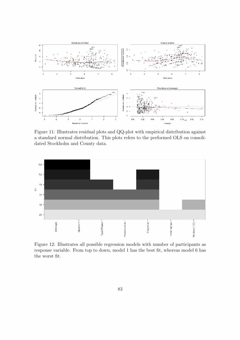
Figure 11: Illustrates residual plots and QQ-plot with empirical distribution againsta standard normal distribution. This plots refers to the performed OLS on consoli-dated Stockholm and County data.

Figure 12: Illustrates all possible regression models with number of participants asresponse variable. From top to down, model 1 has the best fit, whereas model 6 hasthe worst fit.

83

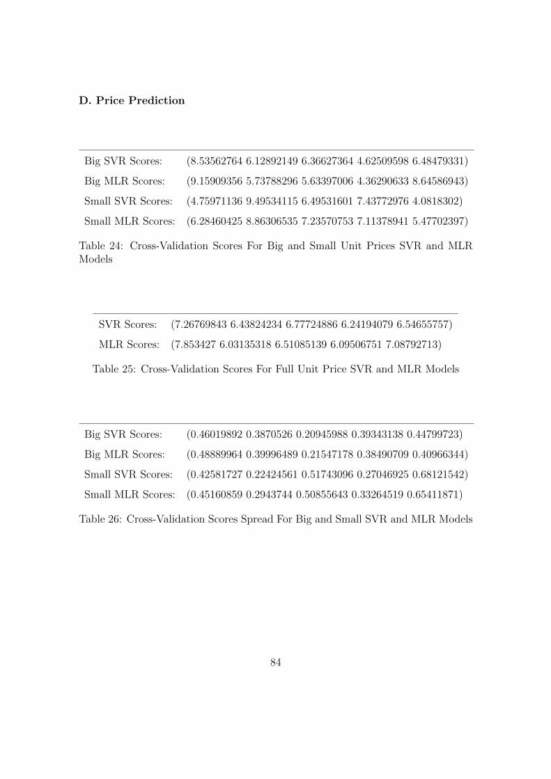
D. Price Prediction

Big SVR Scores: (8.53562764 6.12892149 6.36627364 4.62509598 6.48479331)

Big MLR Scores: (9.15909356 5.73788296 5.63397006 4.36290633 8.64586943)

Small SVR Scores: (4.75971136 9.49534115 6.49531601 7.43772976 4.0818302)

Small MLR Scores: (6.28460425 8.86306535 7.23570753 7.11378941 5.47702397)

Table 24: Cross-Validation Scores For Big and Small Unit Prices SVR and MLRModels

SVR Scores: (7.26769843 6.43824234 6.77724886 6.24194079 6.54655757)

MLR Scores: (7.853427 6.03135318 6.51085139 6.09506751 7.08792713)

Table 25: Cross-Validation Scores For Full Unit Price SVR and MLR Models

Big SVR Scores: (0.46019892 0.3870526 0.20945988 0.39343138 0.44799723)

Big MLR Scores: (0.48889964 0.39996489 0.21547178 0.38490709 0.40966344)

Small SVR Scores: (0.42581727 0.22424561 0.51743096 0.27046925 0.68121542)

Small MLR Scores: (0.45160859 0.2943744 0.50855643 0.33264519 0.65411871)

Table 26: Cross-Validation Scores Spread For Big and Small SVR and MLR Models

84