
Bicyclist Exposure Estimation Using Heterogeneous Demand Data … · vides greater predictive...
70
Bicyclist Exposure Estimation Using Heterogeneous Demand Data Sources by Frank Roland Proulx A dissertation submitted in partial satisfaction of the requirements for the degree of Doctor of Philosophy in Civil and Environmental Engineering in the Graduate Division of the University of California, Berkeley Committee in charge: Professor Alexey Pozdnukhov, Chair Offer Grembek, PhD, Co-chair Professor Joan Walker Professor Michael Anderson Fall 2016
Transcript of Bicyclist Exposure Estimation Using Heterogeneous Demand Data … · vides greater predictive...

Bicyclist Exposure Estimation Using Heterogeneous Demand DataSources
by
Frank Roland Proulx
A dissertation submitted in partial satisfaction of the
requirements for the degree of
Doctor of Philosophy
in
Civil and Environmental Engineering
in the
Graduate Division
of the
University of California, Berkeley
Committee in charge:
Professor Alexey Pozdnukhov, ChairOffer Grembek, PhD, Co-chair
Professor Joan WalkerProfessor Michael Anderson
Fall 2016

Bicyclist Exposure Estimation Using Heterogeneous Demand DataSources
Copyright 2016by
Frank Roland Proulx
1
Abstract
Bicyclist Exposure Estimation Using Heterogeneous Demand Data Sources
by
Frank Roland Proulx
Doctor of Philosophy in Civil and Environmental Engineering
University of California, Berkeley
Professor Alexey Pozdnukhov, Chair
Offer Grembek, PhD, Co-chair
Quantifying risks and the effects of risk factors requires controlling for exposure,or the number of opportunities for the adverse outcome in question to occur. In thecontext of traffic crashes, traffic volumes are frequently used as an exposure measure.Efforts to study bicyclist crash risk have historically been hindered by the lack ofwidespread exposure data. This study presents methods to estimate bicycle trafficvolumes across an entire urban network.
The first major chapter of the dissertation presents a data schema for classifyingbicycle demand datasets. There is an ever-growing abundance of transportation data,with some of the fastest growth seen in realm of non-motorized demand. However,all of the available datasets provide incomplete information about the system. Forexample, some only represent a time series of observations at a single location inspace (automated counters), while others cover all space and time but only representa small subset of the population of people and trips (crowdsourced data). In orderto understand how these heterogeneous sources of information correspond to oneanother, it was deemed necessary to first identify their differences. Six metadatacharacteristics were defined, which are termed the population scope, trip aggregation,temporal scope, temporal resolution, spatial scale, and demographics. Levels aredefined for each dimension, and examples of generic datasets are discussed in termsof their metadata dimension.
The second major chapter of the dissertation presents a method of fusing mul-tiple link-level demand estimates to infer peak-hour bicycle traffic volumes. Whilethe method is agnostic to the specific sources being used, it is presented with acase study of San Francisco, CA using data from regional travel demand models,a smartphone crowdsourcing application, and bikeshare system ridership. The de-
2
fined process entails first converting the datasets to a common format in terms oftheir metadata dimensions, and then fitting these homogenized link-level estimatesto observed counts using a weighted regression technique modeled after Geographi-cally Weighted Regression. The fitting parameters associated with each dataset arehypothesized to vary geospatially, and the means by which this variation occurs iscontrolled by the specified weighting scheme. A distance decay weighting, where ob-servations further from a given location contribute less to the parameter estimates, isfound to produce the best results. Cross-validation is employed for model compari-son and the selection of features and hyperparameter values. It is shown that, on thebasis of cross-validated Root-Mean Square Deviation, that fusing data sources pro-vides greater predictive accuracy than can be achieved using any individual source,and that utilizing localized regression is more predictive than using a single globalparameter for each data set.
The final chapter is about inferring the temporal distribution of traffic based oncontinuous automated count data. Latent Dirichlet Allocation is applied as a signaldecomposition model to identify latent spatio-temporal patterns in the observedcount data, which appear to correspond to coherent activity patterns such as AMcommuting, PM commuting, and midday cycling. Each link’s temporal distributioncan thus be expressed in terms of the extent to which each latent pattern is observedon it. The mixture of these patterns on unobserved links is interpolated using apurely autoregressive model, in contrast to the historically ad hoc methods used todetermine the temporal characteristics of bicycle traffic on unobserved links.
The primary conclusion of this work is that the lack of exposure data should nolonger be considered an insurmountable problem for studying bicycle crashes. Us-ing advanced analytical methods, such as those presented here, in conjunction withthe abundance of new datasets provides a means of generating defensible retrospec-tive volume estimates for the entire network. This dissertation paves the way formany future lines of inquiry, including both refinements upon the methods presentedhere and application of the volume estimates developed here to problems requiringexposure quantities, such as the evaluation of crash risk.

i
To Jaya, for inspiring me through thick and thin.

ii
Contents
Contents ii
List of Figures iv
List of Tables v
1 Introduction 11 Motivation . . . . . . . . . . . . . . . . . . . . . . . . . . . . . . . . . 12 Dissertation Outline . . . . . . . . . . . . . . . . . . . . . . . . . . . 2
2 Literature Review 31 Crash Prediction/Safety Performance Functions . . . . . . . . . . . . 32 Volume Estimation . . . . . . . . . . . . . . . . . . . . . . . . . . . . 53 Crowdsourcing . . . . . . . . . . . . . . . . . . . . . . . . . . . . . . 104 Summary . . . . . . . . . . . . . . . . . . . . . . . . . . . . . . . . . 11
3 Bicycle Demand Data Sources 121 Metadata Schema . . . . . . . . . . . . . . . . . . . . . . . . . . . . . 122 Data Sources . . . . . . . . . . . . . . . . . . . . . . . . . . . . . . . 14
4 Data Fusion: Geographically Weighted Regression 221 Introduction . . . . . . . . . . . . . . . . . . . . . . . . . . . . . . . . 222 Methodology . . . . . . . . . . . . . . . . . . . . . . . . . . . . . . . 233 Case Study Data . . . . . . . . . . . . . . . . . . . . . . . . . . . . . 294 Results . . . . . . . . . . . . . . . . . . . . . . . . . . . . . . . . . . . 325 Discussion . . . . . . . . . . . . . . . . . . . . . . . . . . . . . . . . . 35
5 Temporal Extrapolation based on Signal Decomposition of Con-tinuous Bicycle Volume Data 381 Introduction . . . . . . . . . . . . . . . . . . . . . . . . . . . . . . . . 38

iii
2 Data Sources . . . . . . . . . . . . . . . . . . . . . . . . . . . . . . . 403 Methodology . . . . . . . . . . . . . . . . . . . . . . . . . . . . . . . 404 Results . . . . . . . . . . . . . . . . . . . . . . . . . . . . . . . . . . . 465 Discussion . . . . . . . . . . . . . . . . . . . . . . . . . . . . . . . . . 48
6 Conclusions 531 Contributions . . . . . . . . . . . . . . . . . . . . . . . . . . . . . . . 532 Future Work . . . . . . . . . . . . . . . . . . . . . . . . . . . . . . . . 54
Bibliography 56

iv
List of Figures
3.1 Locations of automated and manual counts in San Francisco, CA. . . . . 153.2 SF-CHAMP estimated trips within each time bin by TAZ . . . . . . . . 183.3 Strava aggregates for weekdays and weekends. . . . . . . . . . . . . . . . 20
4.1 September 2014 PM Peak volume estimates for each dataset. . . . . . . . 304.2 PM Peak bicycle volume estimates from Geographically Weighted Regres-
sion with a Gaussian kernel, 2800 foot bandwidth. . . . . . . . . . . . . . 36
5.1 Latent topic sizes for each hour of the week for K=5 topics. . . . . . . . 475.2 Reconstructed signals from 3 example counters. . . . . . . . . . . . . . . 52

v
List of Tables
4.1 Coefficient of determination matrix for PM Peak volume estimates onobserved links. . . . . . . . . . . . . . . . . . . . . . . . . . . . . . . . . 31
4.2 Comparison of model predictive accuracy for global and local models usingLeave One Label Out Cross-Validation for various combinations of datasources. . . . . . . . . . . . . . . . . . . . . . . . . . . . . . . . . . . . . 33
4.3 Comparison of model predictive accuracy for various link similarity mea-sures in a local model, using SF-CHAMP, Strava Metro, and BABS datasets. 34
5.1 Summary of counting stations, including observed traffic volumes. . . . . 50

vi
Acknowledgments
First, I would like to thank my advisors Professor Alexey Pozdnukhov and Dr. OfferGrembek for being perpetual sources of encouragement, advise, and ideas. Second,my committee members Professors Joan Walker and Michael Anderson for pushingme to make this dissertation the best that it can be.
I would like to also thank everybody in the SafeTREC family. You all do suchinspiring work. In particular, Bob Schneider for being an early and continuing sourceof inspiration. Thanks for keeping me employed while in graduate school.
Further, all of my Cal friends, especially Timothy Brathwaite for always being astep ahead on stats and ready to help, Darren Reger for showing me how to pick upheavy things and keep a balanced life, and Teddy Forscher for helping me to actuallyride bicycles rather than just study abstractions of them. Thanks to Siyu Chen forall of the help with data management - at this rate, you’re going to have finished 5dissertations by the time you finish undergrad.
And, my family. Dad, for passing on the bicycle AND computer science intereststo me from a young age, and for all your help and encouragement along the way.Mom and Lucy, I wish you were still here to see what I’ve accomplished. Mommaand Baba, for loving me as a son. Vipul Bhaiya, for putting me up for TRB everyyear, and the warm welcome into the family.
Above all, thank you to my wonderful wife Jaya. This PhD is an accomplishmentof both of us, and would not be possible without your unending support and patience.We made it!
This research was funded in part by the University of California Center on Eco-nomic Competitiveness in Transportation and the Federal Highway Administration’sDwight D. Eisenhower Fellowship program.

1
Chapter 1
Introduction
Cities, states, and countries around the world are increasingly turning to encour-aging bicycling as a space and energy efficient form of transportation, a means ofpromoting public health through increased activity, and simultaneously are increas-ingly prioritizing traffic safety. For example, the recently released Caltrans StrategicManagement Plan identifies simultaneous goals of a 10% reduction of bicyclist fa-talities per year, an as-yet-unspecified reduction in the number of bicyclist injuries,and a tripling (percentage-wise) of bicycle mode share by 2020 [Brown Jr. et al.,2015]. While well-intentioned, these goals are fundamentally at odds with each otherunless risk to bicyclists is reduced, where “risk” can be understood in a Bernoullitrial sense as the number of expected crashes for a given number of “trial” events. Inthe context of epidemiological studies, such as those looking at traffic safety, thesetrials are often referred to as “exposure” [Hauer, 1982].
1 Motivation
The factors underlying risk, particularly to bicyclists, are not thoroughly understood.When traffic crash prediction models are developed using geographic entities
(such as intersections) as the unit of study, traffic volumes are typically used asa proxy for exposure. In the case of multi-class crash models (e.g. bicycle-motorvehicle; pedestrian-motor vehicle), the expected number of crashes is typically ex-pressed as a function of the volumes of both road user classes in an attempt to controlfor exposure. However, bicycle crash models have historically been hindered by thelack of extensive collection of bicycle volume data. Furthermore, the ideal relation-ship between the two volumes to proxy for exposures has not been well-established,and is further complicated by the fact that the relevant exposure quantity might

CHAPTER 1. INTRODUCTION 2
vary depending on the type of crash under consideration.While many cities in the United States are quickly implementing the collection
of bicycle count data as a routine activity, we can expect that there will continueto be poor coverage of this data for years to come. However, many other sourcesof bicycle demand data are available that, while not providing direct measurementof link-level demand, can be used to help infer volumes across the network. Theseadditional demand data sources include travel demand model estimates, bikeshareusage data, and crowdsourced trip data. Each of these demand data sources aresubject to various strengths and limitations.
2 Dissertation Outline
The remainder of the dissertation is structured as follows. Chapter 2 discusses liter-ature relevant to the questions of bicycle risk evaluation and, as a natural extension,exposure estimation. Following that, the bicycle demand datasets under consider-ation are presented in the context of a novel metadata schema in Chapter 3. InChapter 4, a method for estimating demand during a single time period (in thiscase, the PM peak) by fusing together demand estimates from multiple sources us-ing weighted regression. The initial focus is on the PM peak due to the abundanceof “ground-truth” counts conducted during this period, as many communities relyupon short-duration manual counts for bicycle volume data collection. To get fromthe PM peak to total bicycle traffic volumes, some knowledge of the temporal dis-tribution of traffic on each link must be assumed. In Chapter 5, automated bicyclecount data is decomposed using Latent Dirichlet Allocation (LDA). This analysispresumes that there are latent temporal travel patterns that have some degree ofspatial/directional order to them, which appears to be true. Finally, in Chapter 6some concluding thoughts are presented on the analysis contained herein, includingacknowledgment of limitations and suggestions for future work.

3
Chapter 2
Literature Review
This chapter reviews the literature as relevant to bicyclist risk evaluation. As hasbeen suggested in the Introduction, a critical component of risk evaluation at the sitelevel and the primary focus of this dissertation is the estimation of bicycle volumesas a measure of exposure. The literature review therefore covers both bicycle crashmodels in general and approaches to bicycle volume estimation.
1 Crash Prediction/Safety Performance
Functions
Analyzing traffic crashes is frequently broken into multiple conditional probabilities,with separate models estimated for crash severity (conditional on a crash havingoccurred) and crash frequency Lord and Mannering [2010], Savolainen et al. [2011].When analyzing infrastructural contributors to crash frequency, the location at whichcrashes occurs must be recorded. The most commonly used model for predictingcrash occurrence is the so-called “Safety Performance Function (SPF)”, which ex-presses the expected number of crashes within a given spatial extent (e.g. intersec-tions, road segments) as a function of exposure [Hauer, 1982]. Exposure here refersto a quantification of events that could potentially result in a crash. When workingwith spatially disaggregate crash data, such as using intersections or segments asthe unit of measure, annualized traffic volumes are typically used as a measure ofexposure.
In the context of motor vehicle (single- or multi-vehicle) crashes, an exposuremeasure such as Annual Average Daily Traffic (AADT) is most commonly used.However, when considering multi-class crashes such as between bicycles and motor

CHAPTER 2. LITERATURE REVIEW 4
vehicles, volumes of both vehicle classes need to be taken into account, i.e. controllingfor both AADT and Annual Average Daily Bicyclists (AADB).
Using the number of crashes as an outcome measure suggests a count-regressionmodel, and therefore most studies consider a Poisson-family regression model. Whilemany modifications upon the basic Poisson model have been considered in the traf-fic safety literature (e.g. Negative-Binomial, Zero-Inflated Poisson, Zero-InflatedNegative-Binomial), in all cases the exposure and other risk factors are used to pre-dict the rate parameter of crash occurrence, i.e.:
Ci ∼ Poisson(µi) (2.1)
log (µi) = β0 + β1 log (AADBi) + β2 log (AADTi) +n∑3
βjXij (2.2)
where
Ci = Number of crashes at location (segment or intersection) i
βj = Estimated parameters
Xij = Additional risk factors associated with observation i
There have been relatively few bicycle SPFs developed, due to both the paucityof available exposure data for bicyclists (AADB), and to do the relative rarity ofcrashes. Most cities do not have observed bicycle traffic volumes at a sufficientnumber of locations colocated with crashes to estimate a robust model.
Elvik [2013] identifies three such studies, with two considering intersections andone considering road sections. All three studies document the so-called “Safety-in-Numbers” effect, where the coefficient corresponding to bicycle volumes is less than1. This suggests that as the number of cyclists increases, the expected number ofcrashes per cyclist (and therefore the risk posed to any individual cyclist) decreases.
In addition to simply considering exposure in the SPF, additional risk factorscan be included via the Xj in equation 2.1. For example, Jonsson [2005] considersthe effects of surrounding land uses, visibility, and road class on crash frequency,finding a higher crash risk associated with business districts than residential areas,which is attributed to differences in the relative temporal patterns in bicycle andmotor vehicle traffic volumes. Turner et al. [2009] separately consider various types ofbicycle crashes (e.g. mid-block, mid-block turning, intersection) and find an increasedrisk associated with bicycle lanes for mid-block bicycle-motor vehicle crashes andsignalized intersections. However, it is suggested that this counter-intuitive findingis attributable to a dataset biased towards high crash locations.

CHAPTER 2. LITERATURE REVIEW 5
Strauss et al. [2013] simultaneously estimate bicycle activity levels and bicyclecrash risk at signalized intersections in an attempt to overcome the lack of observedbicyclist exposure and endogeneity between these quantities, finding a positive rela-tionship between the presence of bus stops and total crosswalk length and crashes,and a negative relationship with the presence of raised medians. Notably, the pres-ence of bicycle facilities was not found to have an effect on injury crash frequency.
In summary, existing bicycle crash frequency models have in general not shownstrong evidence of the effect of bicycle facilities on bicycle crash risk. While it ispossible that there is truly no relationship (or a positive relationship), it appearspremature to draw any strong conclusions on the matter due to the severely limitedextent of available data, particularly on bicyclist exposure.
2 Volume Estimation
In order to inform bicycle crash frequency models, estimating bicycle volumes atunobserved locations is an important matter. The question of bicycle volume esti-mation can be subdivided into two dominant paradigms: choice-based, i.e. throughthe assignment of trips to the network using a route choice model based on estimateddemand, and facility-based (“direct-demand models”) Kuzmyak et al. [2014].
Choice-based models
The behavioral approach is a component of larger-scale travel demand models, suchas the fourth step in the “four-step” trip-based modeling framework, or based on thetrips predicted by an activity-based model [McNally, 2008, Bhat and Koppelman,2003]. In either case, trips by various modes of transportation are predicted basedon travel or activity-travel diaries, either for the current “base case” scenario or forforecast conditions. In the activity-based framework, times of day for trips are alsopredicted. These trips can be summarized by an Origin-Destination Matrix (ODM),which includes the estimated number of trips between each Origin-Destination Pairby mode, time of day, trip purpose, and conceivably any other means by which tripscould be subclassified.
One particular difficulty in estimating bicycling demand (especially comparedwith driving and public transit ridership) is the relatively high occurrence of “purerecreation” trips, or trips where there is no “destination” per-say, the trip originand destination are both typically at home, and utility is derived from the act oftravel. For example, a recent mode share survey of San Francisco identified thatout of the 20% of respondents who ever ride a bicycle, approximately 1
4report rid-
CHAPTER 2. LITERATURE REVIEW 6
ing exclusively for recreation [Corey, Canapary & Galanis, 2011]. Various studieshave developed models predicting participation in pure recreational travel, primarilywithin the activity-based framework (which takes into account temporal constraints)[Sener and Bhat, 2012, Bhat and Gossen, 2004]. However, these models often onlypredict the type of recreation to be participated in (i.e. in-home, out-of-home, purerecreation), and do not specifically predict pure recreational bicycle trips, let alonethe characteristics of such trips like distance and route.
Given an ODM, a route choice model is needed to determine link or intersection-level volumes in the trip assignment process. The estimation and application ofroute-choice models is a robust area of research unto itself, with two of the maindifficulties being accounting for correlated errors between routes that use the samelinks of the network, and developing an analytical choice set given that the universalset of routes between two points on a network is virtually uncountable. Ben-Akivaet al. developed one of the most widely used solutions to the first problem, thepath-size logit model, in which route utilities are penalized based on the length-wisedegree of overlap with other routes in the choice set [Ben-Akiva et al., 1984]. Bovyprovides a thorough overview of the choice set development problem [Bovy, 2009].
Numerous bicycle route choice models have been developed using stated-preferencedata or recall interviews (see e.g. [Winters et al., 2010, Kang and Fricker, 2013]).However, with the development of smartphones and affordable GPS transponders,some studies have moved to estimating route choice models based on observed routes,which is not subject to imposing a choice set nor to problems of recall [Broach et al.,2012, Hood et al., 2011].
Broach et al. [2012] distributed GPS transponders to 164 cyclists in Portland, ORand estimated a route choice model based on utilitarian trips, using the Path-SizeLogit adjustment to a Multinomial Logit model. Broach et al. find intuitive effects ofdistance, topography, turns, motor vehicle traffic volumes, and bicycle facility types(as well as some interactions) on route attractiveness to cyclists. Similarly, Hoodet al. [2011] estimate a bicycle route choice model for San Francisco, CA based ondata collected using the San Francisco County Transportation Authority’s “Cycle-tracks” cellphone application and find intuitive effects associated with route length,turn density, wrong way riding, topography, bicycle facilities, including separate pa-rameters for up-slope by gender and trip type (commute vs. non-commute).
The choice-based modeling technique has the strong advantage that it is basedin econometric decision theory, and therefore is formulated around explicit modelsof human behavior. This lends a behavioral interpretation to any model parameterestimates (e.g. one can infer monetary value of time based on the marginal rateof substitution between monetary costs and time in a mode choice model), and isbetter suited to forecasting because of this. However, when the goal of demand

CHAPTER 2. LITERATURE REVIEW 7
estimation is volumes across links or through intersections, direct observations ofthese quantities should be taken into account, which is not directly accommodatedin the choice-based framework.
Facility-based models
As opposed to choice-based models which utilize travel surveys as the primary datainput to infer choice rules for travelers, facility-based models primarily rely on ob-served volumes at discrete locations in space (i.e. along links or through intersec-tions) to estimate activity levels. Facility-based models can further be decomposedinto the tasks of temporal extrapolation and spatial interpolation. Specifically, giventhat the desired exposure measure is Annual Average Daily Bicyclists but manualtraffic counts are frequently taken during a short duration (such as the PM peak),an understanding of how traffic is distributed across time at each location is neededto determine what a particular PM peak traffic volume implies about AADB. Thespatial interpolation question, on the other hand, has to do with inferring how con-sistently measured traffic volumes differ in space.
Temporal Extrapolation
In order to understand the temporal variation in traffic volumes, continuous auto-mated counters are installed at a subset of locations. The Federal Highway Admin-istration’s Traffic Monitoring Guide recommends an approach to temporal extrap-olation known as “factoring,” where the continuous count sites are classified into“factor groups” based on similarities in their temporal profiles Federal Highway Ad-ministration [2013]. The means of the proportions of overall traffic occurring withineach sub-interval (e.g. hour of the day) are found for each factor group, and theseextrapolation factors are used to normalize any short-duration observed volumes.
Sites falling within a common factor group is frequently understood to not be afunction of the magnitude of volumes at the sites, but simply of how those volumesare distributed across time. In practice, multiple continuous count stations withsimilar traffic distribution patterns often have their expansion factors averaged tocreate group averages. Assigning even the continuous count sites to groups, then,despite complete exposition of the patterns at these sites requires some thought.For motorized traffic, the TMG recommends defining factor groups based on federalfunctional road classification. However, this approach is more or less ignorant of thebehavioral basis of travel. For instance, a given city might have two multi-use trails,one through the middle of the city and one on the outskirts. We can imagine thatthese would have very different traffic patterns, with the inner city path carrying a

CHAPTER 2. LITERATURE REVIEW 8
much higher share of commute traffic and therefore having both stronger AM/PMpeaks on weekdays and a higher ratio of weekday:weekend traffic, despite being thesame facility type.
The development of factor groups for bicycle traffic has been previously consid-ered. For example, Miranda-Moreno et al. [2013] consider
, based on data from 37 continuous counters installed in five North American citiesidentifies four factor groups present in the data, and terms them ”Recreational”,”Mixed Recreational”, ”Mixed Utilitarian”, and ”Utilitarian” ascribing a pseudo-behavioral interpretation to the observed patterns. The assignment method in thisstudy involved an iterative manual grouping, where sites were grouped based on hourof day weekday, weekend, and day of week distributions, 95 % Confidence Intervalswere calculated for each group’s distribution, and sites were reassigned based onwhether they fell within the CI or not. Unfortunately, no insight is provided onwhat the underlying cause of these patterns may be nor is any guidance providedon how to assign an additional site to one of the defined classes. Roll [2013] followsa similar methodology using short-term automated counts of 1-2 weeks in Eugene,OR to identify an additional factor group, which he attributes to the presence of amajor university.
Nordback et al. [2013] uses continuous count data from 12 stations in Boulder, COto explore the extrapolation error of calculating AADB using the TMG FactoringMethod based on the amount of “short-duration” count data available, assumingsimply a commute/non-commute grouping, and finds a point of diminishing returnsaround one week of data, with an average absolute percent deviation of 20-30%.Further, extrapolation error is shown to be lowest when the short duration countsare collected when volume variability is lowest, which in their case was between Mayand October.
El Esawey et al. [2013] investigate various methods for calculating daily adjust-ment factors for bicycle traffic volumes based on data from Vancouver, BC, andrecommend using factors specific to each month of the year. Additionally, they findsimilar estimation accuracy when using simple weekday vs. weekend factors com-pared with using a separate factor for each day of the week.
There are a number of problems with the factoring approach for extrapolation.First, it relies upon knowing what group a given site belongs to without havinglong term count data, which is the basis for the groupings. Second, it ignores anydeviations from the systematic time effects due to other factors, namely weather,which has been shown to have a substantial effect on bicycling activity levels.
As mentioned earlier, there are also a number of papers that have explored thetemporal variation in bicycle volumes based on long-term patterns. In the earliestidentified longitudinal analysis of bicycle volumes, Niemeier [1996] explores AM and
CHAPTER 2. LITERATURE REVIEW 9
PM peak period counts from 5 sites in Washington using Poisson regression, and findsgreater variability in the PM peak period than in the AM peak period, negativeassociations between volume and temperature and volume and precipitation, andthat temperature appears to be a stronger predictor of volumes than precipitation.Tin et al. [2012] consider continuous count data from a single counter in Auckland,NZ using ANOVA and OLS regression, and find negative associations between windand rain and bike volumes, and a positive association between maximum temperatureand the presence of sunshine. Gallop et al. [2012] and Nosal and Miranda-Moreno[2014] both extend the multivariate longitudinal analysis of bicycle volumes basedon weather conditions to account for serial autocorrelation, using a Seasonal ARIMAmodel in the case of Gallop et al. and a simpler ARMA model in the case of Nosaland Miranda-Moreno.
Spatial Interpolation
Beyond the task of expanding volume estimates across time, we face the problem ofexpanding across space. Whereas the problem of accounting for temporal variationin volumes is a function of the time and weather, spatial variation in volumes is typ-ically explained (in the facility-based perspective) in terms of characteristics of thesurrounding environment, such as land use, transportation network characteristicsand structure, and sociodemographics. This approach is known as “direct-demandmodeling”, where volumes at a location are regressed on characteristics of the sur-roundings. For instance, a direct-demand model may predict bicycle volumes basedon population density, number of transit stops, and presence of bicycle facilitieswithin a 500-foot radius around the intersection. This approach is tractable and fairlyeasy to estimate, but lacks in behavioral realism when considering bicyclists. Whilethe immediate surroundings of an intersection may be a good predictor of pedestrianvolumes, bicyclists have greater ability to deviate paths (e.g. to preferred facilities)and travel greater differences (e.g. trips may be generated by and attracted to lo-cations far from the intersection, yet still require routing through the intersection).These mechanisms are not captured well by direct demand models. Additionally,“temporal activation” of land uses is not typically considered (e.g. schools shouldonly have a substantial effect on volume during school hours) - rather, all existingmodels either consider a temporally aggregate volume estimate (e.g. AADB), or onlyuse a short-duration count period such as the 2-hour PM peak period.
The majority of published direct demand models for estimating bicycle volumesutilize either short-duration counts or aggregate counts. Regressors are consideredwithin buffers of varying radii, such as 0.1mi, 0.25 mi, and 1.0mi, and are typicallyentered in either an ad hoc, forward stepwise, or backward elimination manner. The
CHAPTER 2. LITERATURE REVIEW 10
regression models used are frequently either an Ordinary Least Squares (linear orlog-linear), or else a count regression (Poisson/Negative Binomial). Basic exampleof bicycle volume direct-demand models include Haynes and Andrzejewski [2010],Griswold et al. [2011] and Lindsey et al. [2006].
One substantial problem with the majority of bicycle volume direct demand mod-els is that they do not account for spatial autocorrelation - that is, they ignorethe spatial quality of the data under consideration. Strauss and Miranda-Moreno[2013] attempts to account for this using an inverse distance weighted spatial lagterm. Count data in this paper are extrapolated to annualized values, accountingfor weather in multiple ways. Additionally, varying impedance values are tested forthe spatial lag term.
3 Crowdsourcing
Crowdsourcing of bicycle demand data entails asking the public to report their trips,typically using GPS-enabled smartphones. This is frequently either done by trans-portation agencies with the primary goal of understanding bicycle demand, as in thecase of the San Francisco County Transportation Authority’s “CycleTracks” applica-tion Hood et al. [2011], or by private companies whose primary product is analyticson exercise patterns for app users, but who have developed a secondary product ofselling anonymized demand data to transportation planning agencies as in the caseof Strava Metro [Strava, Inc., 2014].
Applications of and analytical techniques for crowdsourced bike demand data area nascent field. The are two dominant applications as pertaining to the estimationof link or intersection-level volumes. First, if crowdsourced data are available in adisaggregate, trip-based format, it can be used to estimate a route-choice model,which can then be utilized to assign trip estimates for which only origins and des-tinations are available to the network, as previously discussed [Hood et al., 2011,Broach et al., 2012]. In some cases, such as Strava Metro, trips are not representedby individual traces, but are instead aggregated to link counts which can be taken asa proxy for volume as in Griffin and Jiao [2015]. However, it is possible and indeedquite likely that this crowdsourced data is biased demographically, temporally, andspatially compared to the true aggregate volumes. To make rigorous evaluations oftotal bicycle demand using crowdsourced data requires a thorough understanding ofwhat these biases might be, which is to date not well understood in a general sense.

CHAPTER 2. LITERATURE REVIEW 11
4 Summary
The overall literature gap that this dissertation seeks to make progress towards isthe lack of a thorough understanding of bicycle crash risk factors. One of the biggestreasons for this current gap is the lack of quality exposure data, which in turnrepresents its own gap in the literature. This is where the attention for the remainderof this work will be, and in particular as it pertains to finding a happy median betweenthe current modeling techniques of utility-based travel demand modeling and facilityfocused “direct-demand” modeling, while also taking into account the rapid growthof crowdsourced datasets that are currently ill-understood.

12
Chapter 3
Bicycle Demand Data Sources
In this chapter, I will discuss the variety of spatially referenced bicycle demand datasources available. All forms of bicycle demand data ostensibly measure the same un-derlying phenomenon (people traveling via bicycle across spacetime). However, thereare no perfect sources of spatiotemporally resolved information on travel behavior,with all available datasources suffering censorship temporally or spatially, or biasesin the populations of people or trip types represented. First, I present a metadataschema intended to assist in identifying how the various available demand datasetsrelate to one another and how they might need to be homogenized to enter into acommon predictive framework. Then, I present various demand datasets. For each, Idescribe the type of data source generically, including classification according to theproposed metadata schema. Then, I discuss the particulars of the source as collectedin my case study city of San Francisco, CA, including some exploratory analysis.
1 Metadata Schema
Demand data can be classified based on its collection format and on its representa-tional format. The collection format describes the raw underlying data, while therepresentational format describes the data as available to the modeler. Representa-tional formats are not fixed- that is, demand data can be changed between formats,which is the crux of the method proposed herein. Implicitly, then, some data sourcesmight be considered by the analyst until after processing has been performed (e.g.by the data provider).
The proposed schema categorizes datasets on six metadata dimensions, termedthe population scope, trip aggregation, temporal scope, temporal resolution, spatialscale, and demographics. Each of these will now be discussed in more detail, including
CHAPTER 3. BICYCLE DEMAND DATA SOURCES 13
presentation of possible values that they might take.
Population Scope The population scope defines whether a given dataset is in-tended to represent the full population or a subset of the population, where the “pop-ulation” here is the population of both people and trips. Generally speaking, we areprimarily interested in full population estimates; however, there are relatively fewmethods that are able to capture this. Naturally, when only a subset of the popu-lation is represented we must wonder how this sample relates to the full population,and frequently do not have a strong understanding of this connection.
Trip Aggregation Trips can either be represented as aggregate, cross-tabulatedquantities or as discrete records.
Temporal Scope The temporal scope denotes the extent of data representation,temporally. For example, a given dataset might provide a full historical time-seriesor a partial/truncated historical time-series, where observations are attributed tospecific date-times. Alternatively, one might encounter an average or “typical” time-series, where either a full/partial time-series was aggregated to an average represen-tation or else an estimate was generated to describe the expectations for a recurrenttime period, such as a “normal weekday”. The typical time-series definition couldbe extended beyond the “normal weekday” to account for other factors that mightaffect travel patterns, such as by generating separate estimates for rainy weekdaysand non-rainy weekdays.
Temporal Resolution Whereas the temporal scope details the temporal extentof data, the temporal resolution describes how finely observations have been sliced.There are three primary options for handling this dimension: disaggregate times-tamped observations, aggregation to a fixed binning interval (e.g. 15-minutes), oraggregation to a “semantic” binning pattern where bins are defined according to abehavioral intuition. For example, delineating the AM Peak, Midday Off-Peak, PMPeak, and Evening/Night Off-Peak.
Spatial Scale Travel occurs in space as well as time. Accordingly, the spatialdimension must be captured, which can be done with varying degrees of acuity:
• Site-based observations are taken at discrete locations in space, such as alonglinks or through intersections.

CHAPTER 3. BICYCLE DEMAND DATA SOURCES 14
• Traces are empirical records of routes taken, such as those taken using GPStransponders. These can either be in free-space or “map-matched” to thenetwork.
• Origin-Destination point datasets provide details of the specific start and endpoints of trips, but no indication as to the route taken.
• Origin-Destination zone datasets only expose the approximate start and endlocation of trips, again with no explicit routing. These origins and destinationsare at the scale of the Travel Analysis Zone (TAZ) system used.
Demographics Any additional details about the nature of trips represented arecaptured under demographics. This might include details on the trip-makers (e.g.age, gender, income), helmet-usage status, trip purpose, whether trips were made ina group, or any other characteristics of interest that could be collected.
2 Data Sources
Given that we now have a unifying framework for categorizing bicycle demanddatasets, I will now present some commonly available types of data, as well as spe-cific details of these datasets as they are used throughout this dissertation in a casestudy of San Francisco, CA.
Counts
Traffic counts are collected to evaluate demand at fixed locations in space (i.e. are asite-based measure). They can be collected either on a short-duration or continuousbasis, with automated technologies or by hand, and either at intersections or alongsegments. Counts are intended to be a full-population measure, and any deviationsfrom this are assumed to be random due to counter limitations. In San Francisco,both automated and manual counts have been collected at the locations shown inFigure 3.1. The manual count locations shown here are for the 2014 data collectioneffort, which is used in this dissertation. The automated counters have been installedgradually over time.
Automated
Bicycle counts can be collected with an automated traffic recorder either as a partialtime-series or as a full time-series, depending in part on the particular technology

CHAPTER 3. BICYCLE DEMAND DATA SOURCES 15
Figure 3.1: Locations of automated and manual counts in San Francisco, CA.
CHAPTER 3. BICYCLE DEMAND DATA SOURCES 16
being used [Ryus et al., 2015]. The technologies currently on the market are similarto those used for counting motorized traffic. Continuous (full time-series) countsare collected using induction loops, piezoelectric strips, magnetometers, and radar,with automated video and automated infrared video analysis on the cusp of marketpenetration and adoption. Limited duration counts are most commonly collectedusing pneumatic tubes, although induction loops can also be used in this way. Allof these technologies (with the exception of the two video-based methods) are suitedonly for collecting data across a screenline, meaning that they cannot be used tocollect turning movements. However, they are all capable of collecting directionalcounts.
San Francisco has one of the highest densities of automated bicycle counterswithin a single city. At this time, there are approximately 80 counters installed,although a large proportion of these were installed in the course of the completion ofthis research. These counters are all “induction loops,” similar to those commonlyused for signal actuation at intersections. Induction loop counters are known tooperate very accurately, but are subject to “bypass errors” when their coverage doesnot subtend the entire width of a facility [Ryus et al., 2015]. The counters used inthis study have not been validated for accuracy with respect to bypass errors.
Manual
Manual bicycle counts can either be collected in the field or by reviewing videofootage after the fact. In either case, the primary cost is time spent which scaleswith the extent (temporally and spatially) of data collected. This is in contrast withautomated counters, which effectively have a fixed cost irrespective of the temporalextent of data collected. Accordingly, manual counts are best suited to collecting avery short partial time-series of data, which operationally for many cities amountsto a two-hour count in the AM- or PM-peak.
In San Francisco, an annual PM-peak bicycle count is conducted by volunteers.Counts are collected as turning-movements at a 15-minute temporal resolution. In2014, the year that the analysis conducted in Chapter 4 of this study is based upon,manual counts were conducted at 77 intersections around the city.
Travel Demand Models
Many regional planning organizations and some large cities maintain extensive utility-based travel demand models. These models make use of detailed activity-travelsurveys, typically taken on 5-10 year cycle, where respondents report for a shorttime-period (e.g. 24-48 hours) all of the activities that they engage in, where and

CHAPTER 3. BICYCLE DEMAND DATA SOURCES 17
when these activities took place, and what mode of transportation was taken totravel between activity locations, as well socio-demographic details of the respondentand other members of the respondents’ household. Models used in practice involvevarying degrees of complexity to approximate human behavior, from the traditionalfour-step models to modern activity-based models. These travel demand models areused to evaluate the anticipated effects of various policies and infrastructure modifi-cations, such as the widening of highways, raising of tolls, or addition of bicycle lanes,on overall demand as well as mode splits. “Synthetic populations” of potential trip-makers are generated for the region, and for a given policy/network scenario theirtravel decisions are probabilistically determined according to the demand model.
Modeling of bicycle mode choice in the U.S. context has traditionally been dif-ficult in the utility-based travel demand model framework for a variety of reasons,perhaps most importantly low response rates of bicyclists in travel surveys due to therelatively low bicycle mode share. However, where models do include bicycling as apossible choice in decision-makers choice sets, judgments can be made about bicycledemand for a given scenario. These judgments are often made for a “typical week-day,” which limits the ability to forecast demand for weekends when travel patternsare likely substantially different than on weekdays. Furthermore, the effects of fac-tors such as weather and shifting sunrise/sunset times are not often accommodated,which are likely to have profound impacts on peoples’ decisions to bicycle. Finally,recreational bicycle trips do not fit well into a model based on utility, particularly ifspatial details are desired, and are often not included in these models.
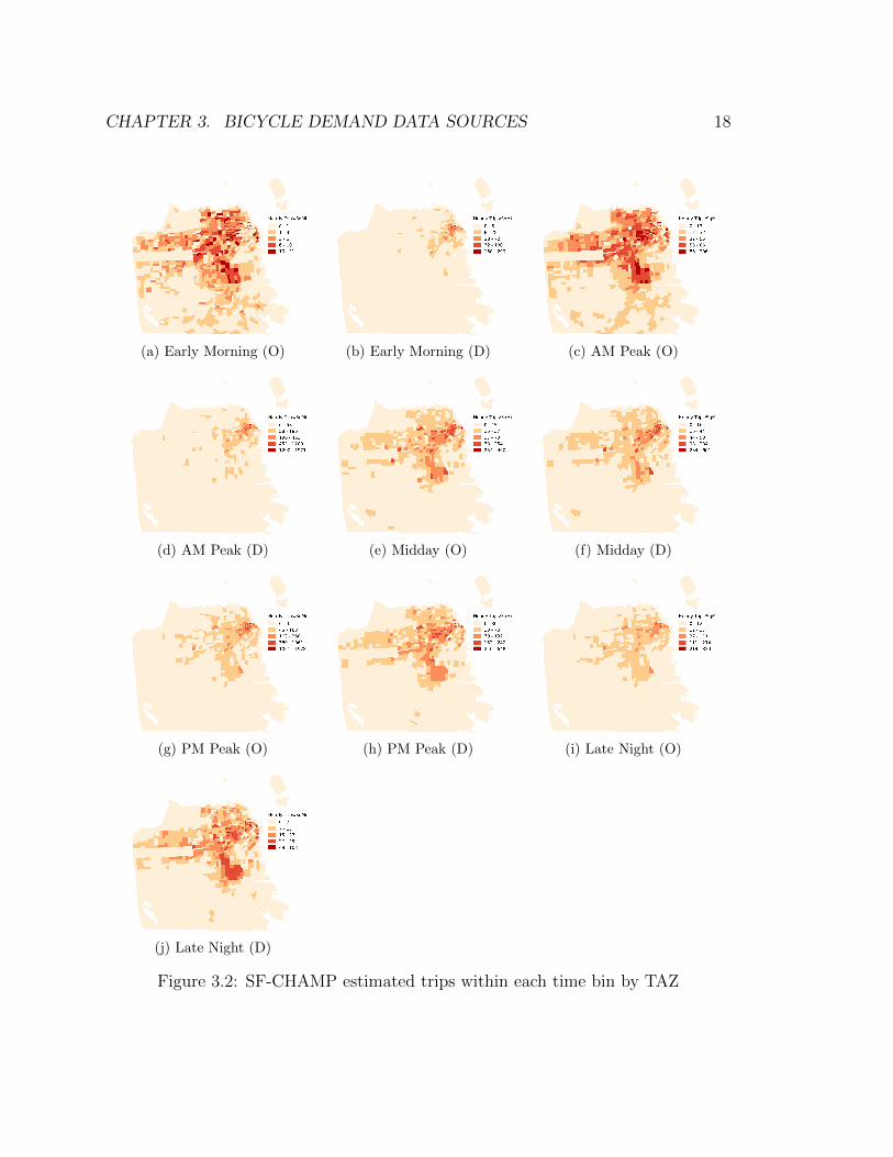
For San Francisco, there are two travel demand models available. Both of theseare activity-based travel demand models, which attempt to model individuals’ entireday schedules and decision processes such that dependencies between individual tripsare maintained. The Metropolitan Transportation Commission (MTC) maintains aregion-wide model on a spatial scale using 1,454 Travel Analysis Zones. The SanFrancisco County Transportation Authority (SFCTA) hosts a more detailed modelof travel patterns within the county of San Francisco using a more fine-grained 2,454TAZ system.
Figure 3.2 depicts the SFCTA’s zonal bicycle demand estimates for both triporigins (“O”) and destinations (“D”) for each of 5 time bins for a “typical weekday”.Note that these panels are internally scaled, meaning that they are not directlycomparable across time periods. The vast majority of the modeled trip destinationsduring the early morning and AM peak time periods are located in downtown, largelyalong the Market Street corridor, but with origins dispersed around the city. For thePM peak period, and late night, the Mission district stands out as a particularlypopular destination.
CHAPTER 3. BICYCLE DEMAND DATA SOURCES 18
(a) Early Morning (O) (b) Early Morning (D) (c) AM Peak (O)
(d) AM Peak (D) (e) Midday (O) (f) Midday (D)
(g) PM Peak (O) (h) PM Peak (D) (i) Late Night (O)
(j) Late Night (D)
Figure 3.2: SF-CHAMP estimated trips within each time bin by TAZ

CHAPTER 3. BICYCLE DEMAND DATA SOURCES 19
Crowdsourced Data
We can consider two different types of crowdsourced bicycle demand data beingcollected, based on the purpose of data collection. The first is “quantified self”smartphone applications where users record bicycle trips, runs, and other work-outs to track their athletic performance. These user-focused applications have hadwidespread uptake due to the benefits they offer to the user. Some companies havebegun selling anonymized usage data, as users have typically not opted in to sharingof their disaggregate data. In terms of transportation planning, this aggregation canbe advantageous, as raw GPS data is burdensome to work with. However, informa-tion is lost in the process on trip-level details, including origins/destinations and usercharacteristics, which makes it difficult to assess how representative a given datasetmight be. The second type of crowdsourced bicycle demand data is research-focuseddata, where the primary purpose of data collection is to support research or planningfunctions.
Strava Metro
Strava is a smartphone application on which users record running and bicyclingtrips that they make, fitting into the “quantified self” realm. Strava Metro isan anonymized data product that Strava sells for planning purposes, where map-matched link-flows of Strava users are recorded on a minute-by-minute basis acrossthe data collection period. These matched flows are directional, and include sepa-rate counts of “athletes” and “activities,” where activities are groups of users whoappear to be traveling together. In addition, separate aggregates are generated for“commute” trips, which are identified based on user tagging of records, having adifferent trip origin and destination (as compared with an “origin-origin” trip), andother similar contextual clues. However, in the extract provided for this case study,the commute counts were not directional, so they could not be separately considered.
There are limited ways that the Strava Metro dataset can be visualized. Similarto in Jestico et al. [2016], the main technique available is to simply filter the datasetto gain insight into how the spatial variation in reported traffic patterns varies basedon the conditions applied. For instance, Figure 3.3 depicts the average daily volumeon all links of the network comparing weekends and weekdays. The dominant fea-tures appear to be similar, although the Weekend traffic does appear to have greatrepresentation on the west half of the city, especially through Golden Gate Park andalong the Great Highway.

CHAPTER 3. BICYCLE DEMAND DATA SOURCES 20
Figure 3.3: Strava aggregates for weekdays and weekends.
Cycletracks
Cycletracks is a smartphone application generated by the San Francisco CountyTransportation Authority to collect cycling trip GPS data for planning purposes[Hood et al., 2011]. Launched in 2009, the platform has been active continuously, withtwo incentivized data collection efforts in 2011 and 2013. Many other communitieshave adopted Cycletracks to collect their own similar data. Users selectively recordbicycle trips that they make, and are prompted to provide the purpose of their tripfrom a drop-down menu. In addition, users are asked (but not required) to providetheir age, gender, cycling frequency, and zip codes of their home, work, and schoollocations. Trips are recorded as GPS traces with 1 second resolution. While thisdataset was considered for inclusion in the studies here, the sample size was deemedtoo small to be useful.
Bikeshare Data
Many cities have recently installed public bikesharing systems. Bikes are stored ata set of fixed-location docking stations, and users are free to check out and returnbicycles to any station with an available dock. Users buy a daily or annual member-ship, and with this membership trips are priced per 30 minute at an increasing rate,
CHAPTER 3. BICYCLE DEMAND DATA SOURCES 21
with the first 30 minutes often being free. This pricing scheme is used to increaseturnover by encouraging users to return their bicycle if it is no longer being ridden.Most systems make their trip records publicly available, and have held competi-tions for creative analysis of their datasets. This is a full time-series of timestampedrecords, with an origin-destination point spatial scale.
Bay Area Bikeshare was launched in 2013, with most of its stations installedaround the financial district and South of Market neighborhoods. This is a fairlyconstrained spatial extent, which limits the inference that can be drawn from thisdatasource.

22
Chapter 4
Data Fusion: GeographicallyWeighted Regression
1 Introduction
As has been argued in Chapter 3, the various available bicycle demand datasetsall have shortcomings in terms of their ability to fully characterize bicycle travelpatterns across the network. While details of travel patterns such as trip purposesdo not necessarily need to be understood in detail for modeling risk, spatial biases intraffic volumes are a critical problem for exposure estimation. These spatial biasescan manifest in many ways, either due to modeling inaccuracies or due to differencesin the types of trips or people being represented by a particular information source.
The goal of this chapter is to fuse together the available demand datasets toovercome these spatial biases and achieve a higher accuracy estimate of link-levelexposure than can be achieved using any individual source. A two step method isproposed. First, datasets are homogenized to a common representation followinga specified series of transformations. This homogenization process is necessary toaccount for differences in how space and time are handled by different sources ofdata.
In the second step, the datasets’ volume estimates are fused together by fittingto observed “ground-truth” counts with a least squares fit. In addition to a standardleast squares fit where the parameter weights are the same everywhere in space,spatially varying coefficients are considered in a method similar to GeographicallyWeighted Regression. In the spatially varying coefficients model, separate parametersare estimated for each link of the network. The variation in these estimates is drivenby applying a weighting scheme to the observations such that observations on links

CHAPTER 4. DATA FUSION: GEOGRAPHICALLY WEIGHTEDREGRESSION 23
that are expected to be similar to the link where estimation is being conductedcontribute more strongly to the loss function than those that are dissimilar. This“similarity” is on the basis of the relative proportion of traffic explained by eachdataset. Although we do not have a means of knowing how similar two links are apriori, various weighting schemes are considered both on the basis of spatial proximity(i.e. weights decay with distance) and on the basis of link characteristics (e.g. roadgeometry).
This chapter focuses on exposure estimation for a single time period (in particular,16h00-19h00 on weekdays) due to the limited availability of ground truth countsoutside of this window. In San Francisco, and in most cities, the majority of availablebicycle count data comes from manual intersection counts performed during the PMpeak. The larger sample size that arises from focusing on this time period allowsfor increased spatial resolution and hence estimation precision. The disadvantage offocusing on this small time window is that it does not tell us anything about theremainder of the week.
2 Methodology
Data Homogenization
The first step in fusing demand data to achieve volume estimates is homogenization interms of trip aggregation, temporal scale, temporal resolution, and spatial scale. Thepopulation scope and demographic variables are typically left untouched, with theexception that one might aggregate across demographics. For a dataset representinga sub-population, we rarely have a thorough understanding of the particular detailsof the sub-population represented, and therefore no basis for extending to a fullpopulation representation. This lack of understanding of the sub-populations is onepiece of the motivation in fusing demand data based on counts, where even “fullpopulation” representing datasets, namely utility-based travel demand models, maynot adequately capture a subset of the types of trips made, such as recreational orfirst/last-mile trips to transit. Generally speaking, homogenization to a lower levelof granularity requires fewer assumptions to be made. I will now detail the procedurefor homogenizing across each of these dimensions.
Trip aggregation
In converting from a disaggregate trip representation to an aggregate trip representa-tion, trips are simply cross-tabulated according to their characteristics on the other
CHAPTER 4. DATA FUSION: GEOGRAPHICALLY WEIGHTEDREGRESSION 24
metadata dimensions (e.g. spatial coordinate, time of day, and mode). To gener-ate disaggregate trips from an aggregate representation, on the other hand, wouldrequire simulation based on our knowledge of the other metadata dimensions. Forexample, suppose that we have a dataset with a 1-hour temporal resolution. Wemight presume a uniform distribution of trip departure times within each hour, andsynthesize individual trips based on this distribution. As noted, converting to thismore granular representation would introduce noise.
Temporal Scope
Three temporal scope representations have been specified, including the full time-series, partial time-series, and average/typical time-series.
Converting from a full time-series to a partial time-series involves truncating theseries to the specified time interval. For example, if we have one dataset which onlycovers a small subset of time, such as a short-duration count taken during the PMPeak period on a given day, we would truncate other dataset time-series’ to matchthis period. To convert from a partial to a full time-series, an assumption wouldneed to be made about how that partial time-series maps to the full unobservedtime-series.
Some sources of demand data refer to a typical or “normal” day. This is par-ticularly common in the case of travel demand models, where the typical conditionsbeing modeled are dependent on the time period in which the underlying travel sur-vey was collected. It is not immediately clear how these average days relate to anygiven day,
Spatial Scale
Converting between differing spatial scales is the most computation intensive com-ponent of this process. Specifically, to convert from an Origin-Destination format(either points or zones) to a site or trace format requires routing trips to the networkbased on a route choice model. Again, this includes making assumptions (ideallyinformed by observations), in this case about how bicyclists make their route choicedecisions. Conversion from a trace format to a site format is commonly termed“map-matching,” as observed GPS traces in raw format must be matched to thenetwork geometry.

CHAPTER 4. DATA FUSION: GEOGRAPHICALLY WEIGHTEDREGRESSION 25
Fitting Procedure
Once a common, site-level volume format is achieved for all datasets, they are fit toobserved counts according to weighted non-negative least squares. Directional linksare the specified unit of analysis. Overall bicycle traffic volumes on each link arepredicted as a linear combination of the volume estimates implied by each of thevarious datasets. That is,
yq = βqvq (4.1)
where
yq = the total bicycle traffic volume on link q
vq = vector of estimated volumes on link q from each dataset
βq = vector of weights dataset weights associated with link q
In other words, the goal is to estimate the weights βq by which each dataset’straffic volume estimates on each link should be scaled to yield the total traffic volumeestimates. It bears noting that these weights have been indexed by the link q, whichwill be discussed shortly.
The idea behind fusing the demand estimates vq is that each dataset yields dif-ferent insight into the aggregate travel patterns, as suggested by the exploratoryanalysis in the previous chapter. For instance, travel demand models are primarilyfocused on predicting utilitarian travel such as commute trips. Crowdsourced smart-phone applications, on the other hand, appear to capture recreational trips whichare not easily predicted by a model.
In using a linear combination of predictions, each data source (i.e. each value inthe vector vq) gets a weight β associated with it. These weights can be interpretedas the component of the aggregate travel that a single cyclist in each data sourcerepresents. For “full-population” datasets such as travel demand models, the idealis that the associated weight is 1, as this would mean that each link count predictedby that dataset corresponds to a single count in the real world.
We hypothesize that the dataset weights could exhibit spatial non-stationarity.That is, the relationship between each dataset’s predicted values and the overalltraffic volume might vary between links. There are a variety of reasons that thisnon-stationarity could occur, such as:
• Lack of coverage for a given dataset on a subset of links (e.g. bikeshare in SanFrancisco only describes travel within a small area of the city where stationslie).

CHAPTER 4. DATA FUSION: GEOGRAPHICALLY WEIGHTEDREGRESSION 26
• Differences in reporting rates based on location (e.g. Smartphone-based report-ing could be biased towards higher income neighborhoods, or towards “recre-ational routes”).
• Biases in route preference for the sub-population being represented (e.g. differ-ent GPS datasets might have differences within their samples in terms of degreeof preference for bicycle facilities, as evidenced by Watkins et al. [2016]).
Allowing the weights to vary arbitrarily on all links would not work, as we wouldencounter an identification problem. To get around this, we draw on a techniqueknown as Geographically Weighted Regression (GWR), following after Fotheringhamet al. [2002]. In general, GWR is specified as:
minimizeβi
∑q
(βivq − yq)2wiq (4.2)
s.t. βi ≥ 0 (4.3)
where
βi = vector of parameters estimated at location i
vq = vector of directional link-volume estimates from set of datasets for link q
yq = observed volume on link q
wiq(α) = weighting factor for regression point i and observation q, controlled by hyperparameters α
As suggested by the spatial variation in the parameters, this regression proceduremust be conducted at each location in space (i.e. link) i where volume estimates aredesired. To implement this, a method for weighting observations has to be specified,which is encapsulated in the term wiq above. The previously suggested identificationissue is avoided here by the weighting scheme. While the weights must vary inspace to yield different results than would be achieved with a standard regressionprocedure, the means by which they vary is controlled by the hyperparameters α,which are set using cross-validation. Once optimal values have been found for α theweights for fitting at each location i are effectively fixed, such that the number offree parameters for fitting at this particular location, the size of βi, is less than thenumber of observations used in their determination.
All that the weights affect, then, is how much each observation on link q con-tributes to the loss function for estimating parameters βi on link i. The specificationof this weighting scheme is generally determined by the analyst, but its specification

CHAPTER 4. DATA FUSION: GEOGRAPHICALLY WEIGHTEDREGRESSION 27
should reflect our beliefs about the nature of the non-stationarity in the data. Linksthat are believed to have similar reporting rates to the regression location ought tobe weighted higher, as the observations on these links can more accurately predictthe dataset weights on the link in question.
Two primary classes of weighting schemes are considered here. The first is thetraditional Geographically Weighted Regression, which expresses weights as a func-tion of the distance between between link i and q. The specific functional form usedis often referred to as the kernel, and here we consider the following:
Gaussian wiq = exp(−1
2(diqh
)2)
Bisquare wiq =
{(1− (
di,qh
)2)2 for di,q ≤ h
0 for di,q > h
where in both cases the bandwidth h is a model hyperparameter that affects theattenuation rate of the distance decay function. In previous work on GeographicallyWeighted Regression, it has been suggested that the specific kernel being used isfar less important than the bandwidth value in terms of predictive accuracy [?].Using a distance-decay weighting scheme supposes that the weights βi are spatiallycontinuous, or in other words that the non-stationarities in their estimates are afunction of location.
The second class of weighting schemes considered here depends on defining mea-sures of “link similarity” between the links i and q. This form conceives that multiplefeatures xiq which relate link i to q can be combined to form an overall similarityscore. Again, two possibilities for this combination are hypothesized here:
• Product: If all features P of xiq are constrained to the range [0, 1) or are binary,wi,q =
∏p∈P xi,q,p
• Logistic: wi,q =exp (α+x′
iqθ)
exp (α+x′i,qθ)+1
where α and θ is are model hyperparameters. One difficulty that arises with usingthe product formulation with multiple binary features is that the set of observa-tions affecting the fit on any particular link decreases (as an increasing number ofobservations receive weights of 0).
The features xiq can be defined using anything that enables comparison betweenlinks i and q, and can be conceived to affect the relative reporting rates of eachdataset. As one example, we could consider an indicator variable for whether ornot links i and q have the same bicycle facility present. If this is included using

CHAPTER 4. DATA FUSION: GEOGRAPHICALLY WEIGHTEDREGRESSION 28
the “product” formulation above, we would get a “hard weighting” whereby theparameter on link i would only be informed by links with the same bicycle facilitypresent. Using the same measure in the “logistic” formulation would instead yield a“soft” weighting where the weights are higher for links with the same facility present,but non-zero for all.
This “hard weighting” approach can also be formulated for cases where there isa known systematic non-response rate in a particular area. For example, bikesharesystem data that only provides origin and destination information cannot tell usanything about travel outside the convex hull of the observed stations. This is anopportune place to apply a hard weight defined by the link lying within the convexhull or not, as without this weighting our estimates for βi would be biased upwardoutside the zone and downward inside the zone.
In addition to specifying these weighting schemes separately, we can also eas-ily combine them by applying both a link similarity measure and a distance-decayweighting. In this approach, the two weighting factors would be interacted. Takingthe bike facility hard weight example again, this would imply that bike lanes near toeach other are more similar than bike lanes further away from each other.
Model Selection and Evaluation
In order to select between model forms and to identify optimal hyperparameter val-ues, leave one label out cross-validation is employed and fit is evaluated on the basisof root mean square deviation (RMSD). Cross-validation is the main criterion usedhere (as opposed to likelihood-ratio tests, for example) because our primary interestis in out-of-sample predictive accuracy [Hastie et al., 2009]. Additionally, becausethe emphasis here is on prediction, not explanation, tests of statistical significancehave not been reported. For more detail than can possibly be given here, see Shmueli[2010] for a comparison of explanatory and predictive modeling.
The “labels” in the cross-validation method refer to the intersections at whichobservations were taken. On each validation fold, all of the observations from agiven intersection are held out as the test set, and the remainder of observationsare used for training. This is done to avoid training and testing on observationstaken from links on the same intersection, which in many cases can be expected tobe highly correlated with each other as all trips through an intersection cross two ofthe intersection’s links.

CHAPTER 4. DATA FUSION: GEOGRAPHICALLY WEIGHTEDREGRESSION 29
3 Case Study Data
Now that the proposed model has been formulated in abstract, we will discuss thespecific data to be used in the case study. The case study focuses on San Francisco,CA during the 4-7 PM period on weekdays in September, 2014. San Francisco wasselected for having a relatively high commute bicycle mode share for American cities(3.5% in 2013, compared with 0.6% nationwide), as well as a wide variety of availabledemand data sources [U.S. Census Bureau]. The PM peak hour is the focus of thisstudy because the majority of available ground truth data comes from manual, peakperiod intersection counts.
Demand Datasets
The demand datasets under consideration have been discussed in detail in Chapter3. To briefly summarize, we are considering the results of two travel demand models(SFCTA and MTC), crowdsourced GPS data (Strava Metro), and usage data fromBay Area Bikeshare (BABS). To homogenize the spatial scale in the case study toa site-based representation, both travel demand models and the bikeshare systemdata must be routed to the network. Routing is performed here using a bicycle routechoice model, generated using GPS traces from San Francisco, and presented in Hoodet al. [2011]. The resulting PM peak volume estimates from each dataset are shownin Figure 4.1.
There are some notable patterns in these volume estimates. First, both theSF-Champ and MTC models are deficient in predicting trips along the northern wa-terfront/across the Golden Gate bridge. This has been traced back to the travelskims (zone-zone distance, time, and cost estimates) used in developing these pop-ulation level demand forecasts, which have trips for zone pairs that would requirecrossing the bridge encoded as infeasible. This is hypothesized to be because thereare relatively low population densities at close proximities on the opposite end of thebridge, so most trips on these zone pairs would have high costs and low populations,and hence a low expected number of utility-based bicycle trips. That is, even if thesetrips were not deemed infeasible prior to model application, the number of estimatedtrips may still be very low. It is also worth noting that the SF-CHAMP and MTCmodels, while both “full-population” estimates, produce vastly different maximumlink volumes - the greatest value on any link suggested by SFCTA’s model is nearlysix times that predicted by the MTC model.
However, it is very well known that bicycling across the Golden Gate Bridge is apopular activity, as documented both by the observed traffic volumes at the bridgeand by Strava Metro. Whereas both travel demand models predict a high densities of

CHAPTER 4. DATA FUSION: GEOGRAPHICALLY WEIGHTEDREGRESSION 30
Figure 4.1: September 2014 PM Peak volume estimates for each dataset.
bicycle traffic in downtown San Francisco, Strava Metro primarily picks up on travelalong the northern waterfront, Market Street, The Wiggle (a popular East-Westbicycle route), and through Golden Gate Park. This difference could be attributable

CHAPTER 4. DATA FUSION: GEOGRAPHICALLY WEIGHTEDREGRESSION 31
to the fact that the volumes in the demand models are a result of routing, andthus are limited to the accuracy of the route choice model, whereas Strava data isobserved and thus indicates the actual routes taken by users. Alternatively, this couldsupport the common hypothesis that Strava data is disproportionately representativeof recreational travel Jestico et al. [2016].
Finally, it is worth noting that the Bikeshare data is limited in spatial scope.The Bikeshare stations in San Francisco are currently limited to a small area focusedaround Market Street, the South of Market neighborhood, and along the Embar-cadero (Eastern waterfront). Because trips are represented on an origin-destinationpoint scale, and thus must be routed to the network to generate volumes, it is unlikelythat the actual volumes exactly match those shown here. That is, these volumes as-sume that travel is direct between the origin and destination. This assumption isa necessity given the nature of the data, and is somewhat justified given that thepricing scheme of the bikeshare system encourages short trips to increase turnover,particularly as this analysis focuses on the the PM peak on weekdays where less than15% of trips are made by non-subscribers.
Table 4.1: Coefficient of determination matrix for PM Peak volume estimates onobserved links.
Observed Volume SFCTA BABS Strava Metro MTC
Observed Volume 1.000 0.348 0.148 0.508 0.011SFCTA 0.348 1.000 0.081 0.045 0.130BABS 0.148 0.081 1.000 0.009 0.000Strava Metro 0.508 0.045 0.009 1.000 0.000MTC 0.011 0.130 0.000 0.000 1.000
In addition to geospatially mapping the volumes predicted by each dataset, wecan consider the pairwise coefficients of determination (R2) between each of thedatasets, and especially with the observed volumes, shown in Table 4.1. This tellsus, if we were to simply linearly scale the estimates from one dataset (and add anestimated intercept term) how well we would predict the other dataset. In the caseof comparing against the ground-truth volumes, this provides some idea as to howwell the dataset matches reality.
We see that the most predictive datasets against the observed volumes are StravaMetro (R2 = 0.508) and the SFCTA data (R2 = 0.347). Interestingly, these datasetsare not very predictive of each other (R2 = 0.045), further supporting the hypothesisthat they are representing different travel patterns, at least for the weekday PM peakperiod under consideration here.

CHAPTER 4. DATA FUSION: GEOGRAPHICALLY WEIGHTEDREGRESSION 32
Weighting Variables
In addition to the demand datasets discussed above, the local model specified hererequires additional variables to inform the weighting matrix component based onlink similarity, wsimi,q . Generally speaking, the features in xi,q can be any categoricalor continuous variables on which links i and q can be compared and are expected tobe related to representation rates of the various datasets. For this case study, thefollowing variables have been considered:
• Bicycle Facility (Categorical): Facility types considered here are “bike path”,“bike lane”, “bike route”, and “None/Unmarked shared lane”.
• Bearing (Continuous): Orientation of the link, based on relative position oflink start and end points.
• Bikeshare Zone (Categorical): Link intersects with the convex hull of the bike-share system stations.
• Street Type (Categorical): Road classification, according to OpenStreetMapscheme: “Primary”, “Secondary”, “Tertiary”, “Residential”, “Cycleway”, “Path”,and “Footway”.
4 Results
The data fusion results section is broken into two main sections. First, tests wereconducted to compare all possible subsets of datasets in terms of predictive accu-racy, using Ordinary Least Squares, a Gaussian distance-decay weighting scheme,and a bisquare distance-decay weighting scheme. For the distance weighted models,searches are performed over a range of possible bandwidth values to find the optimalbandwidth for each subset of data sources. The best prediction is found using theSFCTA model, Strava Metro data, and Bay Area Bikeshare data, weighting obser-vations with a 2500 ft. bandwidth Gaussian kernel. Second, results are shown forexperiments performed on the optimal data sources using various additional weight-ing terms. No substantial improvements to prediction are found here. Finally, theresiduals from the OLS and GWR models are compared to help understand whyprediction is improved with the spatially-varying coefficients model.
Feature Selection
The feature selection results are shown in Table 4.2. The best model, on the basis ofCross-Validation, is a geographically-weighted model with a Gaussian kernel drawing
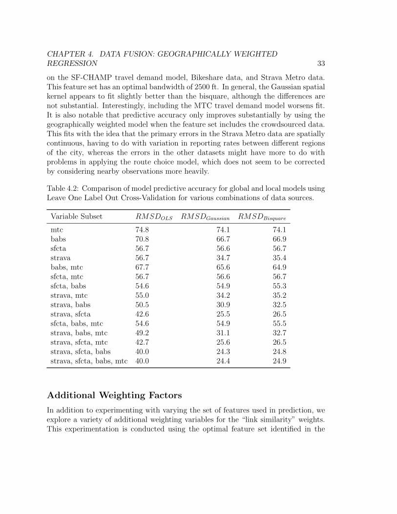
CHAPTER 4. DATA FUSION: GEOGRAPHICALLY WEIGHTEDREGRESSION 33
on the SF-CHAMP travel demand model, Bikeshare data, and Strava Metro data.This feature set has an optimal bandwidth of 2500 ft. In general, the Gaussian spatialkernel appears to fit slightly better than the bisquare, although the differences arenot substantial. Interestingly, including the MTC travel demand model worsens fit.It is also notable that predictive accuracy only improves substantially by using thegeographically weighted model when the feature set includes the crowdsourced data.This fits with the idea that the primary errors in the Strava Metro data are spatiallycontinuous, having to do with variation in reporting rates between different regionsof the city, whereas the errors in the other datasets might have more to do withproblems in applying the route choice model, which does not seem to be correctedby considering nearby observations more heavily.
Table 4.2: Comparison of model predictive accuracy for global and local models usingLeave One Label Out Cross-Validation for various combinations of data sources.
Variable Subset RMSDOLS RMSDGaussian RMSDBisquare
mtc 74.8 74.1 74.1babs 70.8 66.7 66.9sfcta 56.7 56.6 56.7strava 56.7 34.7 35.4babs, mtc 67.7 65.6 64.9sfcta, mtc 56.7 56.6 56.7sfcta, babs 54.6 54.9 55.3strava, mtc 55.0 34.2 35.2strava, babs 50.5 30.9 32.5strava, sfcta 42.6 25.5 26.5sfcta, babs, mtc 54.6 54.9 55.5strava, babs, mtc 49.2 31.1 32.7strava, sfcta, mtc 42.7 25.6 26.5strava, sfcta, babs 40.0 24.3 24.8strava, sfcta, babs, mtc 40.0 24.4 24.9
Additional Weighting Factors
In addition to experimenting with varying the set of features used in prediction, weexplore a variety of additional weighting variables for the “link similarity” weights.This experimentation is conducted using the optimal feature set identified in the

CHAPTER 4. DATA FUSION: GEOGRAPHICALLY WEIGHTEDREGRESSION 34
strictly distance-weighted component. The results have been summarized in Table4.3.
Table 4.3: Comparison of model predictive accuracy for various link similarity mea-sures in a local model, using SF-CHAMP, Strava Metro, and BABS datasets.
Kernel Weighting Link Variables Optimal Parameters RMSD
Gaussian Identity BABS Hull h: 2500 25.4Gaussian Identity Bike Facility h: 3000 28.0Gaussian Identity Bearing h: 2750 24.2Gaussian Identity Highway
Typeh: 3000 29.3
Gaussian Logit Bearing h: 2328α: -2.43θangle: 1.67
24.0
Gaussian Logit BearingBike Facility
h: 2533α: -2.75θangle: 1.16θfacility: 2.01
23.7
— Logit HighwayTypeBike Facility
α: 0.17θhwy: 7.32θfacility: 4.27
39.7
First, we consider simple indicator weights in conjunction with the Gaussiandistance-decay function. Using indicator weights with categorical variables has theeffect that any observations on links that are in the same category as the link wherethe fit is being performed are included, and other sites are not. For example, weight-ing on the “bike facility” variable means that coefficients fit on links with bike lanesonly draw upon observations on links with bike lanes. This supposes that the dataweights βi on link i should only be informed by observations on other links thatshare the specified characteristic with link i. As can be seen in Table 4.3, none of thetested variables substantially improve fit. Part of this could be that by applying thisinclusion/exclusion weighting scheme effectively reduces the sample size for each fitlocation, as dissimilar observations are simply omitted (by applying a weight of 0).
Next, we tested additional weighting formulations that apply a “softer” weightingscheme by utilizing a logistic link function. For example, one such model considersthe relative bearings of the two links on a range of 0 for anti-parallel to 1 for parallelorientations, as well as a separate distance-decay function. To help with interpreting

CHAPTER 4. DATA FUSION: GEOGRAPHICALLY WEIGHTEDREGRESSION 35
this result, consider some examples. Two links that are located at the same locationin space but oriented in opposite directions (i.e. the two sides of a street) wouldcontribute to each other as:
wij = e−12(0/2328)2 exp(−2.43)
1 + exp(−2.43)= 0.08 (4.4)
while two links 500 ft. from each other oriented in the same direction would con-tribute to each others’ data weights as:
wij = e−12( 5002328
)2 exp(−2.43 + 1.67)
1 + exp(−2.43 + 1.67)= 0.977× 0.319 = 0.312 (4.5)
As can be seen in the table, the added complexity of these additional modelsdoes not seem to improve fit. There are a few possible explanations for this. First,we might not have identified the best weighting variables or weighting formulationto correct for small-scale spatial variation in the input data. Second, while extensivecleaning and checking was performed on the input datasets, it is possible that thereare errors in the data that are resulting in a lower limit on the achievable accuracyof the model. That said, these results are of course specific to the datasets used inthis study. In cases where substantial traffic is predicted by a source with a clearcensoring issue (e.g. a more complete bikeshare network), we would expect thatapplying this weighting scheme would work better.
The volume estimates from the optimal geographically weighted model are pre-sented in Figure 4.2. As expected, the underlying patterns of heavy usage along thewaterfront, Market street, through Golden Gate Park, and throughout SoMa appear,although these distinct patterns were not well represented in the maps of individualdataset predictions. The volumes presented here are link totals (i.e. bidirectional),whereas the model predicted values are for each direction on the link separately.
5 Discussion
In this chapter, a novel method has been presented for estimating directional bicyclevolumes on all links of a network for a single time interval based on a variety ofdemand data sources. The proposed method, utilizing Geographically Weighted Re-gression, attempts to overcome spatial differences in reporting rates amongst datasetsby localizing parameters to a given link and weighting observations based on prox-imity. This method has been shown to improve estimation accuracy over using aglobal data weighting scheme.
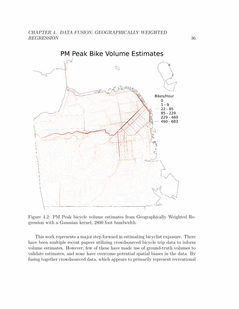
CHAPTER 4. DATA FUSION: GEOGRAPHICALLY WEIGHTEDREGRESSION 36
Figure 4.2: PM Peak bicycle volume estimates from Geographically Weighted Re-gression with a Gaussian kernel, 2800 foot bandwidth.
This work represents a major step forward in estimating bicyclist exposure. Therehave been multiple recent papers utilizing crowdsourced bicycle trip data to informvolume estimates. However, few of these have made use of ground-truth volumes tovalidate estimates, and none have overcome potential spatial biases in the data. Byfusing together crowdsourced data, which appears to primarily represent recreational

CHAPTER 4. DATA FUSION: GEOGRAPHICALLY WEIGHTEDREGRESSION 37
travel in the case study presented, with utility-based travel demand model estimatesand bikeshare data, we have presented a more complete view of directional bicyclevolumes on the network. Furthermore, the methodology presented here is flexibleto additional datasets that may become available in the near future, and provides ameans for evaluating how these datasets fit into the overall representation of travelpatterns.
There are ample opportunities to extend this work. First, within the context ofthe weighted model, we attempted multiple weighting schemes beyond a distancedecay function, such as based on bicycle facility similarity between links. Whilenone of these appeared to improve model fit in this case study, this could still bea useful way forward. Additional weighting schemes might include an estimate ofthe proportion of the trips that pass over the “fit location” and the “observationlocation” based on a trace dataset, or by similarities in surrounding land uses.
Second, we have only considered here spatial variation in the weighting scheme.However, given a greater availability of continuous count data, weights could be con-ceived to also vary temporally when considering panel data. In the case of crowd-sourced data, for example, this might be interpreted as trip reporting rates beinghigher at certain times of the day. Similarly, it would be useful to consider separatemodels for weekdays and weekends, as the bicycle traffic activity patterns are likelysubstantially different on weekends.
Finally, it would be interesting to see how this work replicates in different citiesor across a larger region. The improvements to predictive accuracy noted here byincluding crowdsourced data are due in part to an apparent deficiency in the inputsto the regional travel demand models. While this is a compelling argument for fusingthese data sources together, it is expected that further improvements could be hadin a region with greater variation in facilities, namely a higher preponderance of“primarily recreational” roads. Bicycle volumes on these roads due to recreationaltravel are virtually unpredictable within a utility-based model, but are an importantpart of evaluating risk factors.
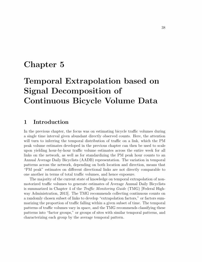
38
Chapter 5
Temporal Extrapolation based onSignal Decomposition ofContinuous Bicycle Volume Data
1 Introduction
In the previous chapter, the focus was on estimating bicycle traffic volumes duringa single time interval given abundant directly observed counts. Here, the attentionwill turn to inferring the temporal distribution of traffic on a link, which the PMpeak volume estimates developed in the previous chapter can then be used to scaleupon yielding hour-by-hour traffic volume estimates across the entire week for alllinks on the network, as well as for standardizing the PM peak hour counts to anAnnual Average Daily Bicyclists (AADB) representation. The variation in temporalpatterns across the network, depending on both location and direction, means that“PM peak” estimates on different directional links are not directly comparable toone another in terms of total traffic volumes, and hence exposure.
The majority of the current state of knowledge on temporal extrapolation of non-motorized traffic volumes to generate estimates of Average Annual Daily Bicyclistsis summarized in Chapter 4 of the Traffic Monitoring Guide (TMG) [Federal High-way Administration, 2013]. The TMG recommends collecting continuous counts ona randomly chosen subset of links to develop “extrapolation factors,” or factors sum-marizing the proportion of traffic falling within a given subset of time. The temporalpatterns of traffic volumes vary in space, and the TMG recommends classifying thesepatterns into “factor groups,” or groups of sites with similar temporal patterns, andcharacterizing each group by the average temporal pattern.

CHAPTER 5. TEMPORAL EXTRAPOLATION BASED ON SIGNALDECOMPOSITION OF CONTINUOUS BICYCLE VOLUME DATA 39
Factor groups are typically established based on the hour-of-day patterns onweekdays, hour-of-day patterns on weekends, and day-of-week patterns. For example,based on these three sub-patterns Miranda-Moreno et al. [2013] identify four factorgroups using induction loop data from multiple cities. These patterns are developedbased on bidirectional traffic and are semantically labeled as “recreational”, “mixedrecreational”, “mixed utilitarian,” and “utilitarian.” This method supposes thatparticular hour-of-day and day-of-week patterns are associated with each other withina given location, which might not necessarily be the case. Further, and perhaps mostimportantly, it does not readily provide a means of identification of the appropriateextrapolation factors for unobserved sites. This is a fundamental omission in the stateof practice that has not been addressed in any systematic way - previous works havematched short-duration count sites to factor groups on the basis of shared facilitytypes and/or common surrounding land uses, but there has been no validation orformal development of these methods [Roll, 2013, Hankey et al., 2014, Nordbacket al., 2013].
As an alternative, in this chapter a decomposition method for link characteriza-tion is presented. The proposed method utilizes Latent Dirichlet Allocation (LDA)for signal decomposition. LDA, originally presented by Blei [2003], is a hierarchi-cal Bayesian model developed for identifying latent topics in text documents. TheLDA model is applied here under the assumption that there exist latent types ofbicycle trips with distinct spatio-temporal patterns associated with them. That is,a given type of trip has a particular probability associated with being observed ata given time of week, and similarly has a varying probability of being observed ondifferent directional links of the network. To be more concrete, an easy example isAM commuting activity which we might suppose has the highest probability of beingobserved between 7 and 9 AM on weekdays, and which is most likely to be observedon links oriented towards the central business district and located in close proximity.
Applying LDA as a signal decomposition tool here, we are able to identify a setof latent bicycle activity patterns. We then develop estimates for the proportionof overall traffic on observed links attributable to each trip type. These weightscan then be used to estimate the overall distribution of traffic on observed links,and on unobserved links if the weights are estimated. Here we present a simplespatial/directional autoregressive model, which infers the mixture weights for thelatent trip types on unobserved links based on the observed signal components onspatially and directionally adjacent links.

CHAPTER 5. TEMPORAL EXTRAPOLATION BASED ON SIGNALDECOMPOSITION OF CONTINUOUS BICYCLE VOLUME DATA 40
2 Data Sources
For this chapter, the primary data source is one week of automated counts collectedbetween June 5 and June 12, 2016 on 75 directional links. Counts were collected using74 bicycle-specific induction loop detectors. Similar to those used to detect and countmotor vehicles, induction loop bicycle counters detect metal objects passing throughtheir detection zone and classify the vehicle according to the currents that it inducesin the loop.
The counters, including the type of facility on which they lie and their observedAverage Daily Bicycle (ADB) volumes during the study period are shown in Table5.1.
3 Methodology
We will now describe the methodology employed for inferring the temporal distribu-tion of traffic volumes across space. The “temporal patterns” referred to here arespecifically the proportion of traffic passing the link within each hour of the weekrelative to all traffic crossing the link in a week. We will denote this fy,t, i.e. thefactor for link y during time-slice t. As these are defined relative to the full week, bynecessity
167∑t=0
fy,t = 1 ∀ y (5.1)
This quantity is observed on a subset of links, but we desire an estimate on all links,so that “peak hour” volume estimates can be appropriately scaled to get volumeestimates for an average day.
There are three main steps to the proposed process:
• Signal Decomposition: Automated count data from the observed links is de-composed using Latent Dirichlet Allocation. For each observed directional link,this results in a set of weights associated with each of the identified latent bicy-cle trip types, as well as a definition of what each of those trip types’ temporalpatterns looks like.
• Spatial Interpolation: In order to infer the trip type proportions on unobservedlinks, we use a fully spatio-directionally autoregressive fractional logit model.
1L: Bike Lane, BL: Buffered Bike Lane, P: Path, CT: Cycletrack, —: No Facility2Average Daily Bicyclists
CHAPTER 5. TEMPORAL EXTRAPOLATION BASED ON SIGNALDECOMPOSITION OF CONTINUOUS BICYCLE VOLUME DATA 41
• Signal Reconstruction: Finally, a process is defined for reconstructing the over-all temporal profile of trips on a given link based on the trip-type proportionsassociated with that link.
Signal Decomposition
In the first step of the proposed method, we seek to decompose the observed temporalbicyclist count patterns on each link into a lower dimensional representation. TheLatent Dirichlet Allocation (LDA) model is employed. LDA is a Bayesian hierarchicalmodel originally developed to identify latent topics in text corpora. In the originalLDA model, it is supposed that we have a corpus of text documents. Each documentis conceived as having a mixture of latent topics underlying it. For each word in eachdocument, a topic is drawn from the document’s topic mixture, and conditional onthis topic a particular word is drawn. Both multinomial distribution parameters aregiven Dirichlet priors.
While LDA was originally conceived in the context of exchangeable text docu-ments, it has also proven useful as a method of decomposing discrete time series datawith multiple parallel signals into underlying components shared across the signals[Coffey and Pozdnoukhov, 2013]. In this application, rather than documents we con-sider time intervals (e.g. hours), which are comprised of a set of discrete observationsat each of a set of locations. In this paper, these observations are bicyclists beingcounted on specific directional links of the network.
LDA was originally conceived as a generative model, meaning that it explicitlymodels the process by which the observations were generated (i.e. for each document,words are drawn from the underlying topic mixture). The analogous generativeprocess for this application is:
1. For each time period t, draw Φ ∼ Dirichlet(α), the distribution of topics withinthe time period t.
2. For each observation of a bicyclist made in time period t:
a) Draw a trip purpose φi ∼ Multinomial(Φ).
b) Draw a link wi from Multinomial(wi|φi, β), which corresponds to the linkwhere the observation occurred.
While this generative story can help elucidate the parallel to topic discovery intext, a probabilistic interpretation provides more intuition on the topic at hand.In this interpretation, for a given time period we have a certain probability of anyobservation arising from a set of trip purposes Z, denoted p(z|t). For example,

CHAPTER 5. TEMPORAL EXTRAPOLATION BASED ON SIGNALDECOMPOSITION OF CONTINUOUS BICYCLE VOLUME DATA 42
during the 8:00 AM hour on a weekday, we might expect a high probability of atrip arising due to AM commuting. We would also expect that particular directionallinks of the network are more likely to have observations occur due to this latent AMcommuting trip type (in particular, links oriented towards downtown would seem tobe a reasonable guess).
Signal Reconstruction
This model as presented is useful for ascribing some meaning to the count observa-tions taken on a set of fully (temporally) observed links. However, it is also useful asa dimensionality reduction tool. Now each observed link can be described in termsof the proportion of the observed bicyclists who are presumed to be a part of eachof the latent trip types. The derivation of this probability will follow.
The output of the Latent Dirichlet Allocation gives us empirical estimates of:
• p(li = y|zi = k) – The conditional probability of link y being drawn for anobservation from topic k.
• p(zi = k|t) – The probability of a given topic k for time period (document) t.
• p(t) – The proportionate size of each time slice t, calculated as Nt∑tNt
, where Nt
is the total number of observations of cyclists in time period t.
From this, we could marginalize out the latent topics Z to get:
p(li|t) =∑k
p(zi = k|t)p(li = y|zi = k)
We should still marginalize out the p(t), yielding:
p(li) =∑t
∑k
p(zi|t)p(li|zi)p(t)
=∑k
p(li|zi)∑t
p(zi|t)p(t)
The overall goal here is to get weights to associate with each topic k for each linky,p(zi = k|li = y), which by Bayes Theorem can be written as:
p(zi|li) =p(li|zi)p(zi)
p(li)(5.2)
While we don’t exactly have p(zi), we can get it from p(zi) =∑
t p(zi|t)p(t).

CHAPTER 5. TEMPORAL EXTRAPOLATION BASED ON SIGNALDECOMPOSITION OF CONTINUOUS BICYCLE VOLUME DATA 43
So, overall, this gives us that:
p(zi|li) =p(li|zi)
∑t p(zi|t)p(t)∑
k p(li|zi)∑
t p(zi|t)p(t)(5.3)
Say that we want to construct the temporal profile for a link y given these weights.Let’s say we have N∗ total observation (i.e. in total across links and time periods).The temporal profile could be written as:
fy,t =Ny,t∑tNy,t
(5.4)
whereNy,t = p(li = y|t)p(t)N∗
bri so
fy,t =p(li = y|t)p(t)∑t p(li = y|t)p(t)
=
∑k p(zi|t)p(li|zi)p(t)∑
t
∑k p(zi|t)p(li|zi)p(t)
=p(t)
∑k p(zi|t)p(li|zi)∑
t p(t)∑
k p(zi|t)p(li|zi)
=p(t)
∑k p(zi|t)p(li|zi)p(li)
(5.5)
The problem in general is that we do not know what p(li|zi) is. But, we canre-express this in terms of p(zi|li) as
p(li|zi) =p(zi|li)p(li)∑t p(t)p(zi|t)
Hence, we can write the temporal distribution fy,t as:
fy,t =p(t)
p(li)
∑k
p(zi|t)p(zi|li)p(li)∑t p(t)p(zi|t)
(5.6)
= p(t)∑k
p(zi|t) p(zi|li)∑t p(t)p(zi|t)
(5.7)
(5.8)
This yields a way to reconstruct the temporal profile given topic probabilities for
each link, but for all unobserved links we will not have p(zi|li = y). Hence, we mustinfer.
CHAPTER 5. TEMPORAL EXTRAPOLATION BASED ON SIGNALDECOMPOSITION OF CONTINUOUS BICYCLE VOLUME DATA 44
Signal Interpolation
At this point, we have decomposed the bicycle counts on a set of observed links into aset of latent trip types, which are defined based on the spatio-temporal patterns un-derlying the data, and determined how to reconstruct the signals given a decomposedrepresentation. The “decomposed representation” referred to here is the proportionof overall traffic on the link attributable to each latent trip type. Re-notating theconditional probabilities as yki = P (zi = k|li)we can refer to the outcome variablematrix as Y which has dimensionality L×K, where L is the number of links and Kis the number of trip types. Our goal here is to estimate yki, which must obey twoconditions:
•∑
k yki = 1 ∀ i
• yki ≥ 0 ∀ k, i
In other words, the vector ~yi must lie on the standardized simplex. The predictionof a simplex outcome variable has been studied previously under the name “frac-tional regression.” One approach to this problem is formulating the outcome vectorY as following a Dirichlet distribution, with the predictor variables linked to theconcentration parameters of the Dirichlet [Woodland, 1979]. However, this provesproblematic if any of the components of the outcome vector take a value of 0 asthe log-likelihood tends towards −∞, which is the case here with some links havingnearly no weekend traffic component. As an alternative, Mullahy [2015] propose theuse of the multinomial logistic distribution, specified with the fractional share as theoutcome variable as opposed to the typical multinomial variable where the predictionis the probability of each discrete outcome occurring.
We will consider a similar formulation here, where we first define:
E[yik|Y, ρ] = ξik ∈ (0, 1), k = 1, ..., K (5.9)
K∑m=1
ξim = 1∀i ∈ I (5.10)
Pr(yk = 0|Y, ρ) ≥ 0, k = 1, ..., K (5.11)
Pr(yk = 1|Y, ρ) ≥ 0, k = 1, ..., K (5.12)
(5.13)
As in Mullahy [2015], we’ll first specify that
E[yik|Y, ρ] = ξik =egk(Y;ρk)∑k e
gk(Y;ρk)(5.14)

CHAPTER 5. TEMPORAL EXTRAPOLATION BASED ON SIGNALDECOMPOSITION OF CONTINUOUS BICYCLE VOLUME DATA 45
where gk(•) relates the observation of yik on link i to observations Y on all otherlinks J through the use of a spatial weighting matrix W . As in most spatial modelingcontexts, the weighting matrix must be exogenously specified, which will be discussedshortly. We also have options to consider for the form of gk(•). The most generaloption here would be to specify
gk(Y ,ρ) = αk +K∑m=1
J∑j=1
wijyjmρmk (5.15)
where
αk = Topic-specific constant for k. Must be fixed to 0 for one topic, e.g. αK = 0
wij = spatial weight relating link j to link i
yjm = observation of topic m on link j
ρmk = spatial autocorrelation between topic m and topic k
This is overly general, with potentially K2 free parameters within ρ. To makethis tractable, we will start with some simplifying assumptions on ρ. First, we mightspecify that ρmk = δmkρk; that is, assume that there are no cross-topic terms inthe spatial autocorrelation. A further, more restrictive assumption would be thatρmk = δmkρ, implying that spatial auto-correlation is constant across topics.
Taking the first of these assumptions, our specification for expected topic shareswould thus be:
ξik =eαk+
∑j wijyjkρk∑
m eαm+
∑j wijyjmρm
(5.16)
Similar to in the Geographically Weighted Regression models presented in Chap-ter 4, a specification for the weighting matrix Wij is required. For a first cut, we’llconsider a joint Gaussian distance decay and angular deviation parameterization,where the element relating observation j to location i is:
wij =
{e−(
dijh
)2 6 βangleij , for i 6= j
0, for i = j
where
6 ij = is the normalized angular deviation between the oreintation of link i and link j
βangle = is a free parameter for the weight given to the angular deviation
h = is the bandwidth for the Gaussian kernel
dij = is the distance between link i and link j
CHAPTER 5. TEMPORAL EXTRAPOLATION BASED ON SIGNALDECOMPOSITION OF CONTINUOUS BICYCLE VOLUME DATA 46
Leave One Out cross-validation is utilized here to find the hyperparameters forthe weighting matrix. Kullback-Leibler Divergence is considered for the loss-function,where fit is evaluated between the modeled and observed latent trip type shares onthe held-out links.
4 Results
Applying LDA to the automated bicycle count dataset results in a set of latent travelpatterns that can be attributed to underlying similarities in their spatio-temporalcharacteristics. The degree to which each of these latent temporal patterns revealsitself on a particular directional link of the network is presumably a function of acomplex assortment of factors, most importantly land use patterns “upstream” and“downstream” of the count location. In this section, we present the observed patternsto reveal their temporal and spatial characteristics. We also hypothesize about whatthese observed patterns might correspond to in terms of bicyclist behavior, althoughfully understanding the underlying causes is not critical to the primary purpose ofthis chapter which is to infer the normalized temporal patterns on unobserved linksof the network.
Decomposition on links with automated counts
The results of the LDA decomposition of automated counts can be visualized invarious ways. First, we can consider the latent topic sizes within each time period,shown in Figure 5.1. Utilizing four topics, we uncover what appear to be an AMcommuting pattern, a PM commuting pattern, a weekday pattern, and a midweekmidday pattern. The “midday” pattern appears to also include some late nightactivity, which would fit with a hypothesized social cause of this activity.
In addition to visualizing the temporal distributions of the identified latent triptypes, visualizing the spatial patterns of topic mixture weights can be informative.In Figure ??, the relative share of counts on each observed link that has been prob-abilistically attributed to each of the latent topics is visualized. This geographicvisualization lends further credence to the interpretation of the latent patterns, aswe can see where in space and direction each trip type is most heavily represented.
For example, Figures ??(a) and ??(b) show the “AM Commute” and “PM Com-mute” patterns, the temporal profiles of which are shown in Figure 5.1. As canbe seen, the travel pattern which we attribute to morning commuting (based on thetimes of day during which it is most prevalent) generally comprises the greatest shareof overall travel on the links that are oriented towards downtown and located close to

CHAPTER 5. TEMPORAL EXTRAPOLATION BASED ON SIGNALDECOMPOSITION OF CONTINUOUS BICYCLE VOLUME DATA 47
Figure 5.1: Latent topic sizes for each hour of the week for K=5 topics.
downtown. Similarly, we see the complementary evening commute patterns the moststrongly on the same links in the opposing direction, out of downtown and particu-larly along the East - West direction. These patterns are very readily interpretableas arising due to weekday commuting behavior.
The other three topics identified here, termed “Midday”, “Evenings”, and “LateNight” are slightly less clear, but we can still hypothesize based on the spatio-temporal patterns. “Midday” occurs most prominently on weekends, with a biastowards the morning, as well as on weekdays during the midday. Spatially, this pat-tern has its most weight along the northern waterfront, as well in the western halfof the city. This suggests some combination of recreational riding and lunchtime so-cial activity. The “Evenings” pattern naturally has its strongest showing during theevening, particularly on weekends. This spatiotemporal pattern appears especiallyprominent on links near to and oriented away from the Golden Gate Bridge, sug-gesting that this may primarily be return trips from trips across the bridge, makingit the complement to the “Midday” pattern similar to the duality of the AM/PMcommute patterns. Finally, the “Late Night” activity pattern occurs most heavilylate at night/in the early morning. This pattern does not comprise a particularlystrong share of overall traffic on any particular link, which is not surprising given theoverall relatively low amount of activity during these hours.
For all of the links with automated counters, we can consider how well the re-construction of the signal performs (based on known topic shares) by plotting thereconstructions and the observed patterns as is shown in Figure 5.2. These plotsdepict the fraction of overall weekly bicycle traffic traversing the links within eachhour. The volumes decomposed onto each latent topic are produced here by scal-
CHAPTER 5. TEMPORAL EXTRAPOLATION BASED ON SIGNALDECOMPOSITION OF CONTINUOUS BICYCLE VOLUME DATA 48
ing the overall topic-specific patterns (i.e. those in Figure 5.1) by the empiricallydetermined conditional topic weights for each link p(zi|li). Importantly, the recon-structed overall signals, shown by the dotted grey lines, reasonably well reproducethe observed signals (solid grey lines).
Inference on spatial distribution of trip types
In addition to visualizing the latent patterns that appear to underly the time seriessignals from automated bicycle counters around the city, we also seek to infer thetemporal distributions of traffic on unobserved links. As discussed in the methodol-ogy, this spatial inference is performed here using a purely autcorrelational model,where all variation in topic patterns is explained by observed variation in the samepatterns on nearby links. The autocorrelation weighting matrix hyperparametersare first set using Leave One One cross-validation and a grid search across potentialvalues, and the lowest average KL-Divergence is found for a bandwidth value of ap-proximately h = 10000ft. with a bearing parameter value of 1.75. The fact that thebearing parameter value is greater than one fits with expectations - this implies thatlinks being closer to parallel than anti-parallel are asymetrically more similar to eachother. In other words, links that “more or less” point in the same direction are moreexplanatory than those that are not, for equal deviations from perpendicular. Withthese hyperparameter values, the spatial autocorrelation coefficient has an estimatedvalue of ρ = 0.64
5 Discussion
This chapter has presented a novel method for accounting for the spatiotemporalpatterns underlying bicycle count data by using a signal decomposition method.These results have both theoretical and practical implications.
Theoretically, the identified latent trip patterns appear to correspond to partic-ular types of travel. This method therefore can be used to provide some insight intothe categories of travel underlying over bicycle traffic patterns, and by visualizingthe latent topic proportions we can see what these dynamics look like across the city.
Practically, we have provided a new means of defining factor groups for purposesof extrapolating short-duration traffic volume estimates to daily averages, as well asfor inferring traffic volumes across the week. While these factor group assignmentshave historically been performed in an ad hoc manner, by decomposing the referencecount site observations into sub-patterns that are assumed to have some spatial and
CHAPTER 5. TEMPORAL EXTRAPOLATION BASED ON SIGNALDECOMPOSITION OF CONTINUOUS BICYCLE VOLUME DATA 49
directional contiguity associated with them, we have shown a means of inferringpatterns based on surrounding observed patterns, rather than rules of thumb.
There are opportunities for improvement at various stages of the proposed model.First, the signal decomposition model could be improved by accounting for depen-dencies in space and time. For example, rather than drawing a topic mixture inde-pendently for each time period with a Dirichlet prior, topic weights within a giventime periods could be used to inform priors for the subsequent time period. Thisaccounting for temporal dependence might help to smooth the decomposed signalsshown in Figure 5.1, and further cement the interpretation of the latent topics astemporally types of travel. Similarly, correlation between links could be accountedfor in the formulation of the conditional link probabilities.
In addition, the spatial inference component as currently specified relies purelyon spatial and directional autocorrelation to infer topic mixture components on eachdirectional link. This could be improved upon by taking into account additionalregressors, such as similarly identified temporal patterns within the other availablebicycle demand datasets or land use variable as in a direct-demand model.
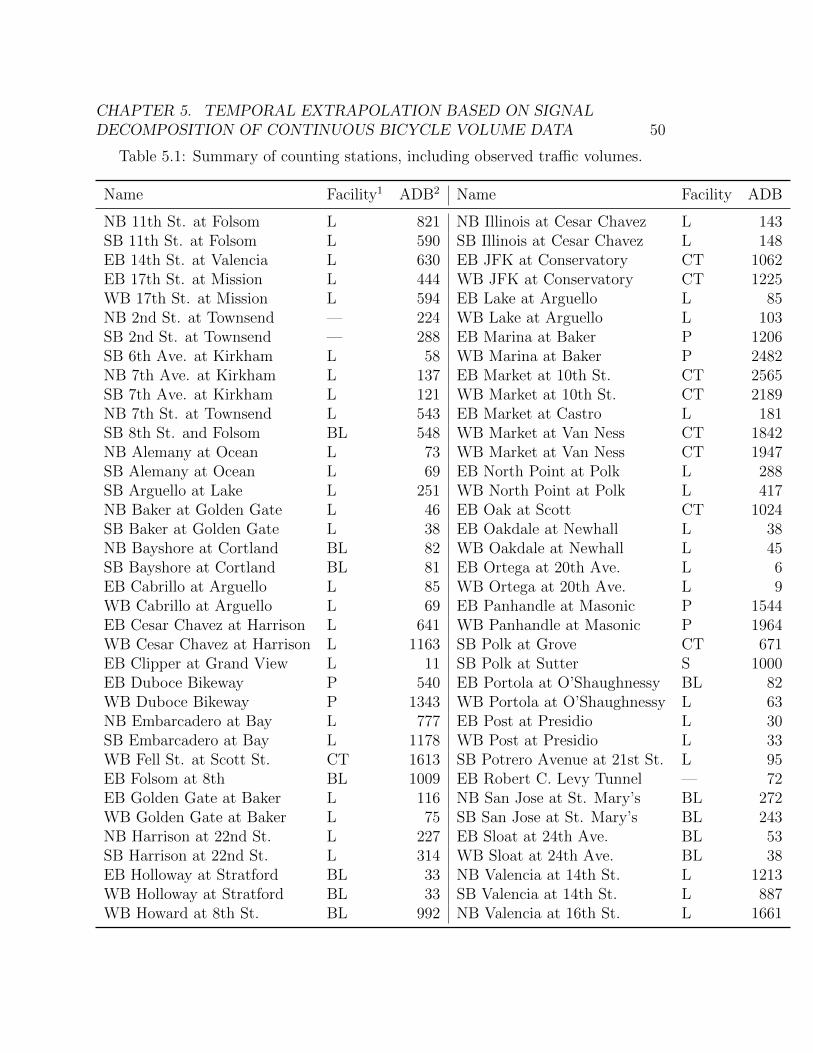
CHAPTER 5. TEMPORAL EXTRAPOLATION BASED ON SIGNALDECOMPOSITION OF CONTINUOUS BICYCLE VOLUME DATA 50
Table 5.1: Summary of counting stations, including observed traffic volumes.
Name Facility1 ADB2 Name Facility ADB
NB 11th St. at Folsom L 821 NB Illinois at Cesar Chavez L 143SB 11th St. at Folsom L 590 SB Illinois at Cesar Chavez L 148EB 14th St. at Valencia L 630 EB JFK at Conservatory CT 1062EB 17th St. at Mission L 444 WB JFK at Conservatory CT 1225WB 17th St. at Mission L 594 EB Lake at Arguello L 85NB 2nd St. at Townsend — 224 WB Lake at Arguello L 103SB 2nd St. at Townsend — 288 EB Marina at Baker P 1206SB 6th Ave. at Kirkham L 58 WB Marina at Baker P 2482NB 7th Ave. at Kirkham L 137 EB Market at 10th St. CT 2565SB 7th Ave. at Kirkham L 121 WB Market at 10th St. CT 2189NB 7th St. at Townsend L 543 EB Market at Castro L 181SB 8th St. and Folsom BL 548 WB Market at Van Ness CT 1842NB Alemany at Ocean L 73 WB Market at Van Ness CT 1947SB Alemany at Ocean L 69 EB North Point at Polk L 288SB Arguello at Lake L 251 WB North Point at Polk L 417NB Baker at Golden Gate L 46 EB Oak at Scott CT 1024SB Baker at Golden Gate L 38 EB Oakdale at Newhall L 38NB Bayshore at Cortland BL 82 WB Oakdale at Newhall L 45SB Bayshore at Cortland BL 81 EB Ortega at 20th Ave. L 6EB Cabrillo at Arguello L 85 WB Ortega at 20th Ave. L 9WB Cabrillo at Arguello L 69 EB Panhandle at Masonic P 1544EB Cesar Chavez at Harrison L 641 WB Panhandle at Masonic P 1964WB Cesar Chavez at Harrison L 1163 SB Polk at Grove CT 671EB Clipper at Grand View L 11 SB Polk at Sutter S 1000EB Duboce Bikeway P 540 EB Portola at O’Shaughnessy BL 82WB Duboce Bikeway P 1343 WB Portola at O’Shaughnessy L 63NB Embarcadero at Bay L 777 EB Post at Presidio L 30SB Embarcadero at Bay L 1178 WB Post at Presidio L 33WB Fell St. at Scott St. CT 1613 SB Potrero Avenue at 21st St. L 95EB Folsom at 8th BL 1009 EB Robert C. Levy Tunnel — 72EB Golden Gate at Baker L 116 NB San Jose at St. Mary’s BL 272WB Golden Gate at Baker L 75 SB San Jose at St. Mary’s BL 243NB Harrison at 22nd St. L 227 EB Sloat at 24th Ave. BL 53SB Harrison at 22nd St. L 314 WB Sloat at 24th Ave. BL 38EB Holloway at Stratford BL 33 NB Valencia at 14th St. L 1213WB Holloway at Stratford BL 33 SB Valencia at 14th St. L 887WB Howard at 8th St. BL 992 NB Valencia at 16th St. L 1661

CHAPTER 5. TEMPORAL EXTRAPOLATION BASED ON SIGNALDECOMPOSITION OF CONTINUOUS BICYCLE VOLUME DATA 51
(a) AM Commute (b) PM Commute
(c) Midday (d) Evenings
(e) Late Night

CHAPTER 5. TEMPORAL EXTRAPOLATION BASED ON SIGNALDECOMPOSITION OF CONTINUOUS BICYCLE VOLUME DATA 52
Figure 5.2: Reconstructed signals from 3 example counters.

53
Chapter 6
Conclusions
1 Contributions
This dissertation has pursued practical solutions to a long-standing problem in thefield of traffic safety; namely, the lack of bicyclist exposure estimates (i.e. trafficvolumes) across an entire street network. The increasingly widespread availability ofhigh quality, spatially and temporally resolved data on bicycle demand has enabledthe solutions proposed herein. In particular, here we have considered fusing trafficvolume estimates from travel demand models, crowdsourced data, and bikeshare sys-tem data. Once reasonable peak-hour volume estimates are available, predicting theunderlying temporal distribution of traffic at all locations is necessary for achievingannual daily traffic estimates.
The specific contributions of this dissertation are as follows:
1. Identified a “test case” location in San Francisco, CA with a relative abundanceof bicycle demand data. This study site could easily be used for future similarstudies.
2. Defined a metadata schema for use in classifying transportation demand data.The proposed schema is useful in defining how distinct datasets relate to oneanother.
3. Developed a data fusion method, based on Geographically Weighted Regres-sion, that can be used to estimate peak period traffic volumes across an entirenetwork. Improved predictive accuracy is shown for this model over a simpler“global” model, and over using any individual dataset independently.
CHAPTER 6. CONCLUSIONS 54
4. Reconsidered the typical formulation of “factor groups” as is promulgated inthe Traffic Monitoring Guide by applying Latent Dirichlet Allocation as a di-mensionality reduction tool to permanent bicycle counter data. This novelformulation provides greater insight into the underlying mechanisms of tem-poral traffic patterns, and allows for more fine-tuned prediction of temporalpatterns on a directional basis.
2 Future Work
This dissertation is just one step in using the ever-increasing abundance of data onbicycling to inform policy. Naturally there are ample opportunities for future work,which can be categorized as refinements upon the methods presented herein andlogical next steps.
For the data fusion method presented in Chapter 4, the formulation of the weight-ing matrix could be revisited. Here, two distance-decay weighting schemes wereexperimented with, as well as some simple “similarity index” weights based on ob-servations coming from locations with the same bicycle facility or road classification.More sophisticated similarity indices would be a worthwhile next step to see if ad-ditional refinements can be made in predictive accuracy. As more datasets becomeavailable, such as additional crowdsourcing streams, they can easily be incorporatedinto the proposed framework to improve estimates.
The temporal decomposition piece discussed in Chapter 5 also has room for im-provement. At the signal decomposition stage, we have here assumed independenceboth between time periods and between network links. Naturally, we might expectthat the probability of observed bicycle counts arising from a particular latent travelpattern might be correlated across time, and that links in close adjacency to oneanother would have similar correlation structures in terms of the their usage by tripsunder a common trip type. The refinement in the temporal dimension could bemade by assuming a random walk process across time periods. The structure acrossdirectional links, however, is less intuitively clear, as this relationship should ideallybe governed both by spatially proximity and directional similarity. One possibilitymight be to utilize GPS traces to inform this relationship. At the signal interpolationstage, at this point only autocorrelation has been used for prediction. Inclusion of ad-ditional regressors, such as land uses surrounding the count site or temporal patternsintimated by the additional demand datasets could potentially improve prediction ofthe topic shares.
Aside from these refinements to the model implementations shown here in SanFrancisco, application to regions with more variation in road types and functions

CHAPTER 6. CONCLUSIONS 55
could be interesting. Specifically, the inclusion of more suburban and rural environscould exemplify the power of the data fusion approach taken here, as part of theunderlying strength of this approach is presumed to be the lack of knowledge ofrecreational bicycle demand in regional travel demand models, and this type of rid-ing is disproportionately prevalent on rural roads. Similarly, the temporal patternspresent in this wider scope of places might benefit more from the temporal decom-position used here than at locations entirely within a fairly dense city, and providemore insight into the underlying predictors of these variations.
The natural next step of this work is to apply the exposure estimates developedherein to evaluating risks incurred by cyclists, especially due to crashes and airpollution. Because the exposure estimates developed here are both spatially andtemporally resolved, novel analytical methods are enabled, including studying boththe spatial factors affecting risk (such as roadway geometries and specifically bicyclefacilities) and temporal factors such as variations in crash risk between night andday and variations in exposure to pollution across space and time.
While very promising results have been shown here in San Francisco, this studylocation was selected in part due to its abundance of available datasets. An addi-tional future line of study would be to develop guidance for communities looking toapply these methods on how to allocate scarce data collections budgets, between con-ducting additional ground-truth counts, improving travel demand models, collectingor purchasing crowd-sourced data, and installing GPS transponders on bikesharesystem bicycles. The relative value of these sources in terms of their informationcontributions towards exposure estimation could be evaluated.

56
Bibliography
M. Ben-Akiva, M.J. Bergman, A.J. Daly, and R. Ramaswamy. Modeling inter-urban route choice behavior. In Proceedings of the 9th International Symposiumon Transportation and Traffic Theory, VNU Press, Utrecht, pages 299–330, 1984.
Chandra R. Bhat and Rachel Gossen. A mixed multinomial logit model analysisof weekend recreational episode type choice. Transportation Research Part B, 38:767–787, 2004.
Chandra R. Bhat and Frank S. Koppelman. Handbook of Transportation Science,chapter Activity-Based Modeling of Travel Demand, pages 39–65. Springer US,2nd edition, 2003.
Andrew Y. Jordan Michael I. Blei, David M. Ng. Latent dirichlet allocation. TheJournal of Machine Learning Research, 3:993–1022, 2003.
Piet H.L. Bovy. On modelling route choice sets in transportation networks: A syn-thesis. Transport Reviews, 29(1):43–68, 2009.
Joseph Broach, Jennifer Dill, and John Gliebe. Where do cyclists ride? a route choicemodel developed with revealed preference gps data. Transportation Research PartA: Policy and Practice, 46, December 2012.
Edmund G. Brown Jr., Brian P. Kelly, Malcolm Dougherty, and Kome Ajise. Caltransstrategic management plan 2015-2020. Technical report, California Department ofTransportation, 2015.
Cathal Coffey and Alexei Pozdnoukhov. Temporal decomposition and semantic en-richment of mobility flows. In LBSN’13 at 21st ACM SIGSPATIAL GIS, 2013.
Corey, Canapary & Galanis. Mode Share Survey 2011: Summary Report. Technicalreport, San Francisco Municipal Transportation Agency (SFMTA), 2011.
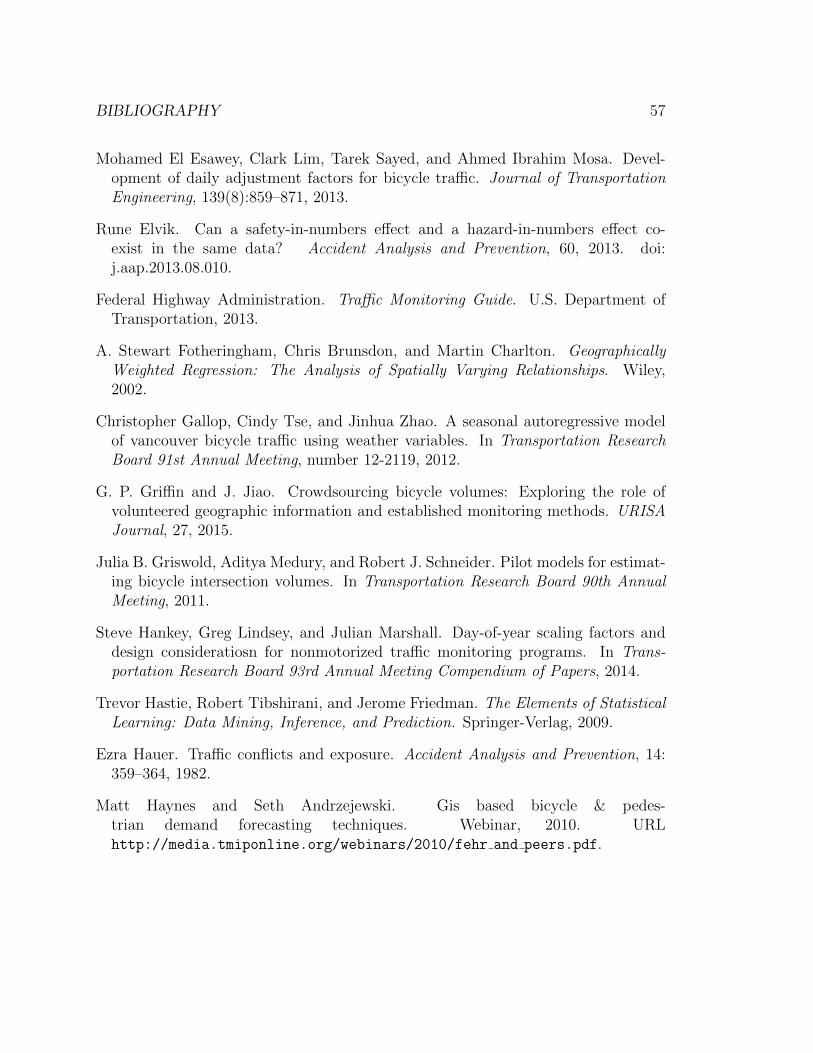
BIBLIOGRAPHY 57
Mohamed El Esawey, Clark Lim, Tarek Sayed, and Ahmed Ibrahim Mosa. Devel-opment of daily adjustment factors for bicycle traffic. Journal of TransportationEngineering, 139(8):859–871, 2013.
Rune Elvik. Can a safety-in-numbers effect and a hazard-in-numbers effect co-exist in the same data? Accident Analysis and Prevention, 60, 2013. doi:j.aap.2013.08.010.
Federal Highway Administration. Traffic Monitoring Guide. U.S. Department ofTransportation, 2013.
A. Stewart Fotheringham, Chris Brunsdon, and Martin Charlton. GeographicallyWeighted Regression: The Analysis of Spatially Varying Relationships. Wiley,2002.
Christopher Gallop, Cindy Tse, and Jinhua Zhao. A seasonal autoregressive modelof vancouver bicycle traffic using weather variables. In Transportation ResearchBoard 91st Annual Meeting, number 12-2119, 2012.
G. P. Griffin and J. Jiao. Crowdsourcing bicycle volumes: Exploring the role ofvolunteered geographic information and established monitoring methods. URISAJournal, 27, 2015.
Julia B. Griswold, Aditya Medury, and Robert J. Schneider. Pilot models for estimat-ing bicycle intersection volumes. In Transportation Research Board 90th AnnualMeeting, 2011.
Steve Hankey, Greg Lindsey, and Julian Marshall. Day-of-year scaling factors anddesign consideratiosn for nonmotorized traffic monitoring programs. In Trans-portation Research Board 93rd Annual Meeting Compendium of Papers, 2014.
Trevor Hastie, Robert Tibshirani, and Jerome Friedman. The Elements of StatisticalLearning: Data Mining, Inference, and Prediction. Springer-Verlag, 2009.
Ezra Hauer. Traffic conflicts and exposure. Accident Analysis and Prevention, 14:359–364, 1982.
Matt Haynes and Seth Andrzejewski. Gis based bicycle & pedes-trian demand forecasting techniques. Webinar, 2010. URLhttp://media.tmiponline.org/webinars/2010/fehr and peers.pdf.
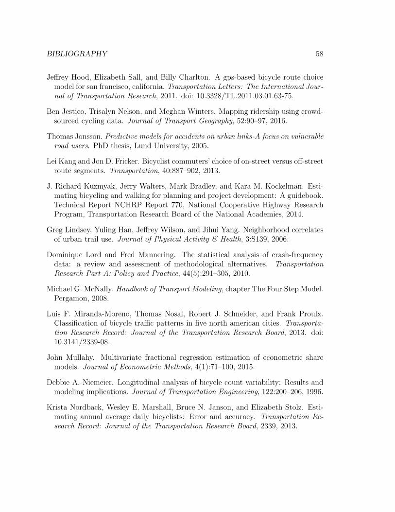
BIBLIOGRAPHY 58
Jeffrey Hood, Elizabeth Sall, and Billy Charlton. A gps-based bicycle route choicemodel for san francisco, california. Transportation Letters: The International Jour-nal of Transportation Research, 2011. doi: 10.3328/TL.2011.03.01.63-75.
Ben Jestico, Trisalyn Nelson, and Meghan Winters. Mapping ridership using crowd-sourced cycling data. Journal of Transport Geography, 52:90–97, 2016.
Thomas Jonsson. Predictive models for accidents on urban links-A focus on vulnerableroad users. PhD thesis, Lund University, 2005.
Lei Kang and Jon D. Fricker. Bicyclist commuters’ choice of on-street versus off-streetroute segments. Transportation, 40:887–902, 2013.
J. Richard Kuzmyak, Jerry Walters, Mark Bradley, and Kara M. Kockelman. Esti-mating bicycling and walking for planning and project development: A guidebook.Technical Report NCHRP Report 770, National Cooperative Highway ResearchProgram, Transportation Research Board of the National Academies, 2014.
Greg Lindsey, Yuling Han, Jeffrey Wilson, and Jihui Yang. Neighborhood correlatesof urban trail use. Journal of Physical Activity & Health, 3:S139, 2006.
Dominique Lord and Fred Mannering. The statistical analysis of crash-frequencydata: a review and assessment of methodological alternatives. TransportationResearch Part A: Policy and Practice, 44(5):291–305, 2010.
Michael G. McNally. Handbook of Transport Modeling, chapter The Four Step Model.Pergamon, 2008.
Luis F. Miranda-Moreno, Thomas Nosal, Robert J. Schneider, and Frank Proulx.Classification of bicycle traffic patterns in five north american cities. Transporta-tion Research Record: Journal of the Transportation Research Board, 2013. doi:10.3141/2339-08.
John Mullahy. Multivariate fractional regression estimation of econometric sharemodels. Journal of Econometric Methods, 4(1):71–100, 2015.
Debbie A. Niemeier. Longitudinal analysis of bicycle count variability: Results andmodeling implications. Journal of Transportation Engineering, 122:200–206, 1996.
Krista Nordback, Wesley E. Marshall, Bruce N. Janson, and Elizabeth Stolz. Esti-mating annual average daily bicyclists: Error and accuracy. Transportation Re-search Record: Journal of the Transportation Research Board, 2339, 2013.
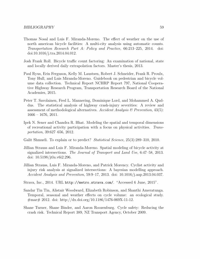
BIBLIOGRAPHY 59
Thomas Nosal and Luis F. Miranda-Moreno. The effect of weather on the use ofnorth american bicycle facilities: A multi-city analysis using automatic counts.Transportation Research Part A: Policy and Practice, 66:213–225, 2014. doi:doi:10.1016/j.tra.2014.04.012.
Josh Frank Roll. Bicycle traffic count factoring: An examination of national, stateand locally derived daily extrapolation factors. Master’s thesis, 2013.
Paul Ryus, Erin Ferguson, Kelly M. Laustsen, Robert J. Schneider, Frank R. Proulx,Tony Hull, and Luis Miranda-Moreno. Guidebook on pedestrian and bicycle vol-ume data collection. Technical Report NCHRP Report 797, National Coopera-tive Highway Research Program, Transportation Research Board of the NationalAcademies, 2015.
Peter T. Savolainen, Fred L. Mannering, Dominique Lord, and Mohammed A. Qud-dus. The statistical analysis of highway crash-injury severities: A review andassessment of methodological alternatives. Accident Analysis & Prevention, 43(5):1666 – 1676, 2011.
Ipek N. Sener and Chandra R. Bhat. Modeling the spatial and temporal dimensionsof recreational activity participation with a focus on physical activities. Trans-portation, 39:627–656, 2012.
Galit Shmueli. To explain or to predict? Statistical Science, 25(3):289–310, 2010.
Jillian Strauss and Luis F. Miranda-Moreno. Spatial modeling of bicycle activity atsignalized intersections. The Journal of Transport and Land Use, 6:47–58, 2013.doi: 10.5198/jtlu.v6i2.296.
Jillian Strauss, Luis F. Miranda-Moreno, and Patrick Morency. Cyclist activity andinjury risk analysis at signalized intersections: A bayesian modelling approach.Accident Analysis and Prevention, 59:9–17, 2013. doi: 10.1016/j.aap.2013.04.037.
Strava, Inc., 2014. URL http://metro.strava.com/. “Accessed 6 June, 2015”.
Sandar Tin Tin, Alistair Woodward, Elizabeth Robinson, and Shanthi Ameratunga.Temporal, seasonal and weather effects on cycle volume: an ecological study.#mar# 2012. doi: http://dx.doi.org/10.1186/1476-069X-11-12.
Shane Turner, Shane Binder, and Aaron Roozenburg. Cycle safety: Reducing thecrash risk. Technical Report 389, NZ Transport Agency, October 2009.
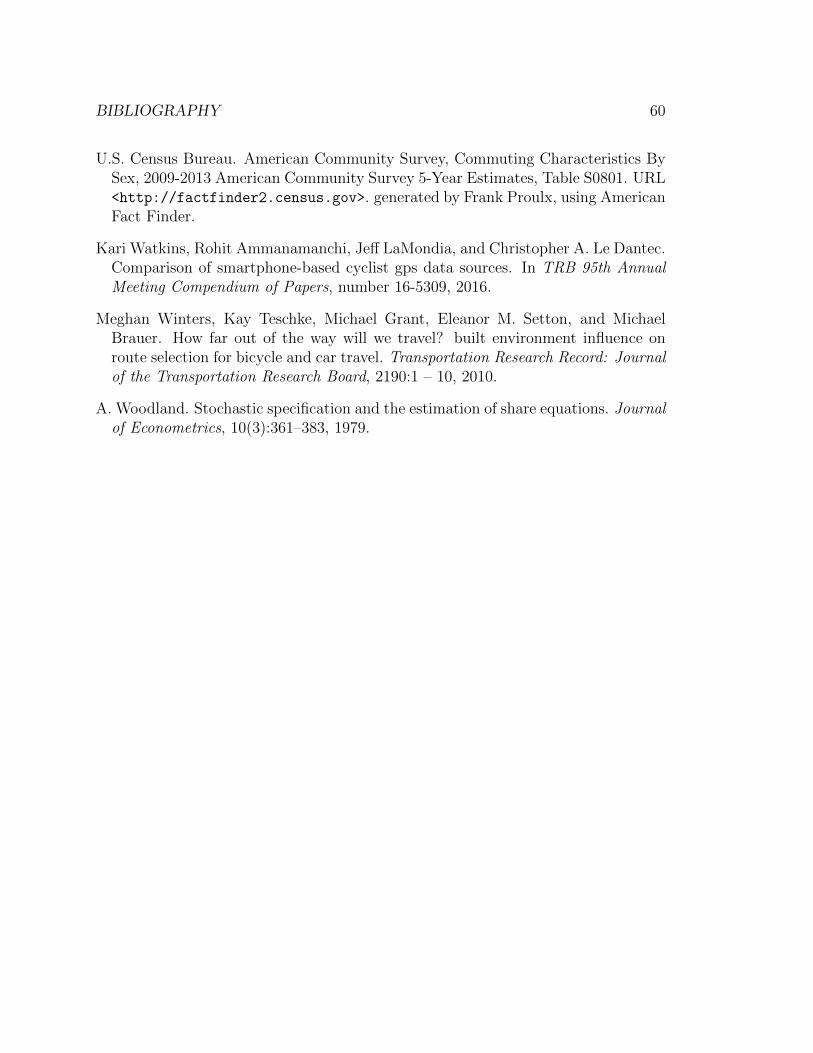
BIBLIOGRAPHY 60
U.S. Census Bureau. American Community Survey, Commuting Characteristics BySex, 2009-2013 American Community Survey 5-Year Estimates, Table S0801. URL<http://factfinder2.census.gov>. generated by Frank Proulx, using AmericanFact Finder.
Kari Watkins, Rohit Ammanamanchi, Jeff LaMondia, and Christopher A. Le Dantec.Comparison of smartphone-based cyclist gps data sources. In TRB 95th AnnualMeeting Compendium of Papers, number 16-5309, 2016.
Meghan Winters, Kay Teschke, Michael Grant, Eleanor M. Setton, and MichaelBrauer. How far out of the way will we travel? built environment influence onroute selection for bicycle and car travel. Transportation Research Record: Journalof the Transportation Research Board, 2190:1 – 10, 2010.
A. Woodland. Stochastic specification and the estimation of share equations. Journalof Econometrics, 10(3):361–383, 1979.