The WeatherResearch & Forecasting Model

WRF

Laura Bianco

ATOC 7500: Mesoscale

Meteorological Modeling Spring 2008

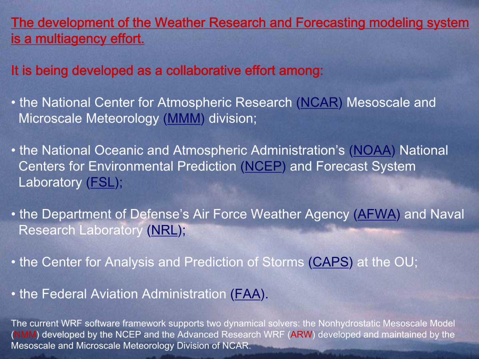
The development of the Weather Research and Forecasting modeling

system is a multiagency effort.

It is being developed as a collaborative effort among:

• the National Center for Atmospheric Research (NCAR)

Mesoscale

andMicroscale

Meteorology (MMM)

division;

• the National Oceanic and Atmospheric Administration’s (NOAA)

NationalCenters for Environmental Prediction (NCEP)

and Forecast SystemLaboratory (FSL);

• the Department of Defense’s Air Force Weather Agency (AFWA)

and NavalResearch Laboratory (NRL);

• the Center for Analysis and Prediction of Storms (CAPS)

at the OU;

• the Federal Aviation Administration (FAA).

The current WRF software framework supports two dynamical solvers: the Nonhydrostatic

Mesoscale

Model (NMM) developed by the NCEP and the Advanced Research WRF (ARW) developed and maintained by the Mesoscale

and Microscale

Meteorology Division of NCAR.

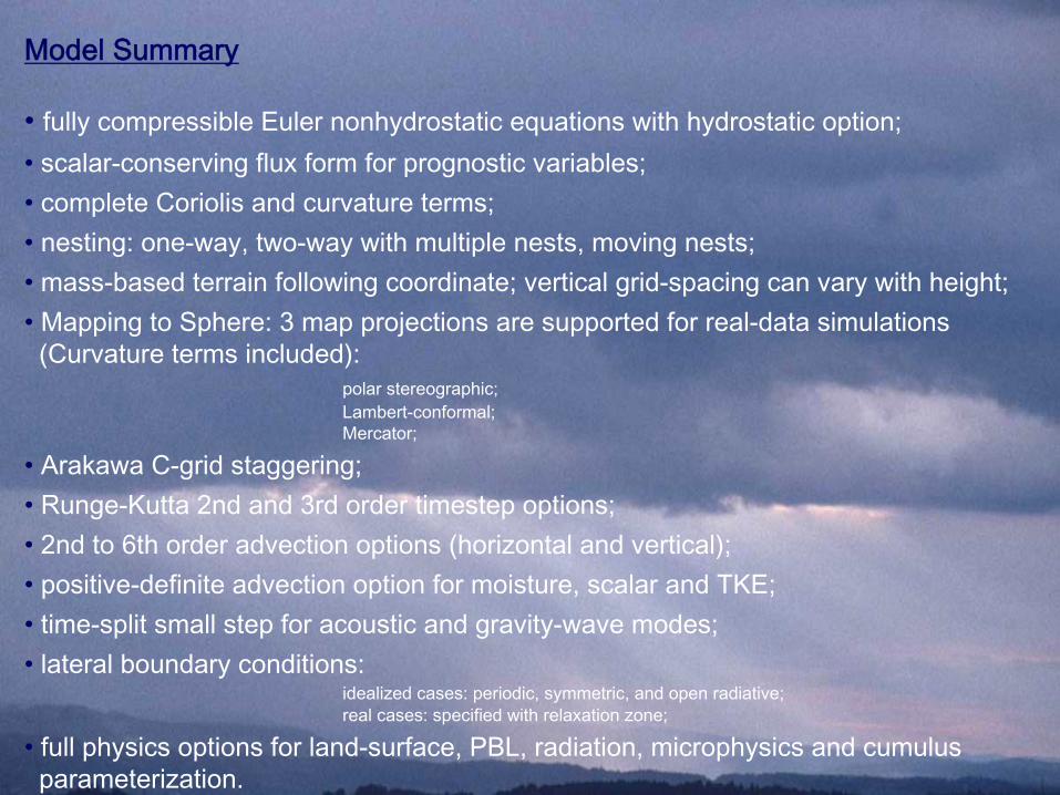
Model Summary

• fully compressible Euler nonhydrostatic

equations with hydrostatic option;• scalar-conserving flux form for prognostic variables;• complete Coriolis

and curvature terms;• nesting: one-way, two-way with multiple nests, moving nests; • mass-based terrain following coordinate; vertical grid-spacing can vary with height; • Mapping to Sphere: 3 map projections are supported for real-data simulations (Curvature terms included):

polar stereographic;Lambert-conformal;Mercator;

• Arakawa C-grid staggering; • Runge-Kutta

2nd and 3rd order timestep

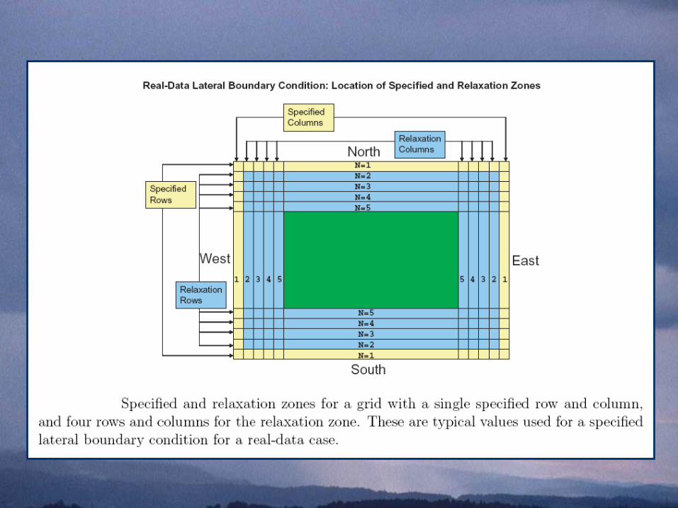
options; • 2nd to 6th order advection options (horizontal and vertical); • positive-definite advection option for moisture, scalar and TKE; • time-split small step for acoustic and gravity-wave modes; • lateral boundary conditions:

idealized cases: periodic, symmetric, and open radiative;real cases: specified with relaxation zone;

• full physics options for land-surface, PBL, radiation, microphysics and cumulusparameterization.

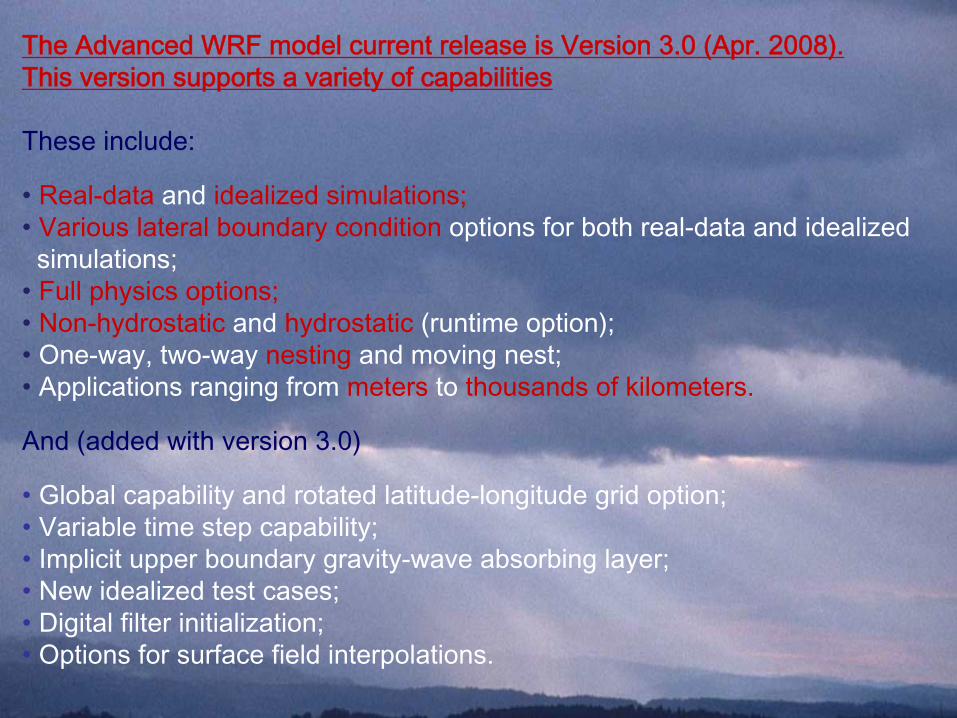
The Advanced WRF model current release is Version 3.0 (Apr. 2008).This version supports a variety of capabilities

These include:

• Real-data

and idealized simulations;• Various lateral boundary condition

options for both real-data and idealizedsimulations;

• Full physics options;• Non-hydrostatic

and hydrostatic

(runtime option);• One-way, two-way nesting

and moving nest;• Applications ranging from meters

to thousands of kilometers.

And (added with version 3.0)

• Global capability and rotated latitude-longitude grid option;• Variable time step capability;• Implicit upper boundary gravity-wave absorbing layer;• New idealized test cases;• Digital filter initialization;• Options for surface field interpolations.

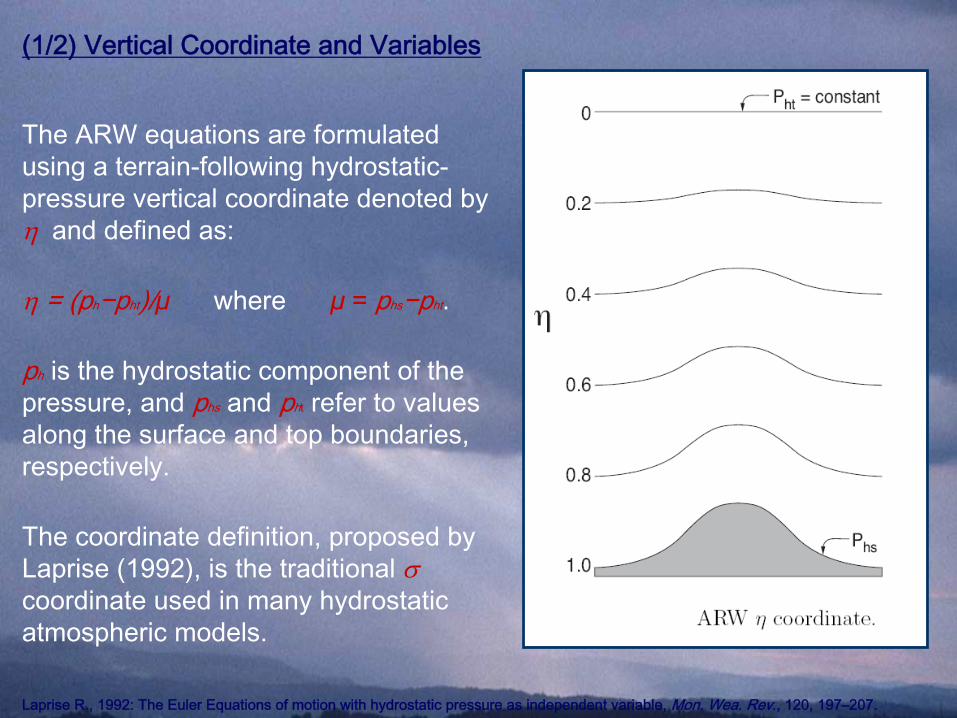
(1/2) Vertical Coordinate and Variables

The ARW equations are formulated using a terrain-following hydrostatic-

pressure vertical coordinate denoted by η and defined as:

η = (ph

−pht

)/μ

where

μ

= phs

−pht

.

ph

is the hydrostatic component of the pressure, and phs

and pht

refer to values along the surface and top boundaries, respectively.

The coordinate definition, proposed by Laprise

(1992), is the traditional

σ

coordinate used in many hydrostatic atmospheric models.

Laprise

R., 1992: The Euler Equations of motion with hydrostatic pressure as independent variable, Mon. Wea. Rev., 120, 197–207.

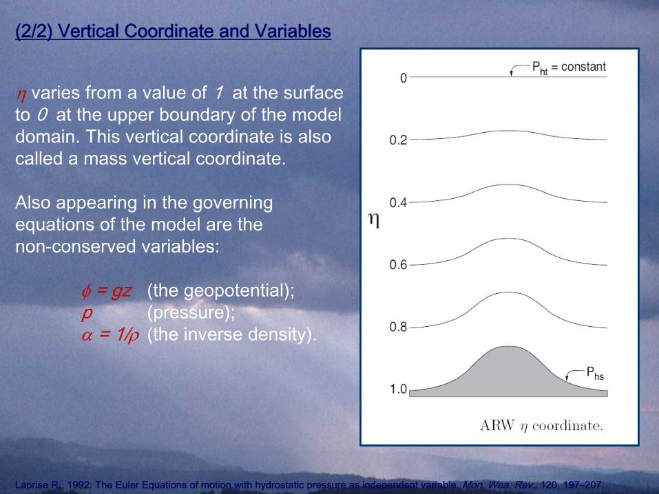
(2/2) Vertical Coordinate and Variables

η varies from a value of 1 at the surface to 0 at the upper boundary of the model domain. This vertical coordinate is also called a mass vertical coordinate.

Also appearing in the governing equations of the model are thenon-conserved variables:

φ = gz

(the geopotential);p

(pressure);α = 1/ρ (the inverse density).

Laprise

R., 1992: The Euler Equations of motion with hydrostatic pressure as independent variable, Mon. Wea. Rev., 120, 197–207.

Equations

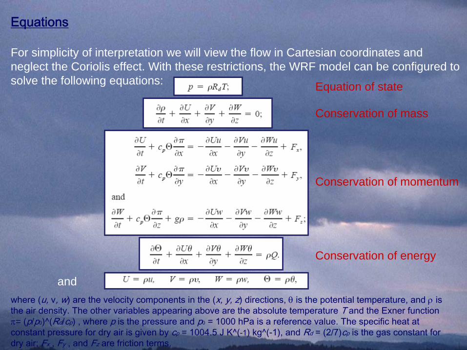
For simplicity of interpretation we will view the flow in Cartesian coordinates and neglect the Coriolis effect. With these restrictions, the WRF model can be configured to solve the following equations:

andwhere (u, v, w) are the velocity components in the (x, y, z) directions,

θ

is the potential temperature, and

ρ

is the air density. The other variables appearing above are the absolute temperature T and the Exner

functionπ= (p/p0

)^(Rd/cp) , where p is the pressure and p0

= 1000 hPa

is a reference value. The specific heat at constant pressure for dry air is given by cp = 1004.5 J K^(-1) kg^(-1), and Rd = (2/7)cp is the gas constant for dry air; Fx , Fy , and Fz are friction terms.

Conservation of momentum

Equation of state

Conservation of mass

Conservation of energy

Runge-Kutta

Time Integration Scheme

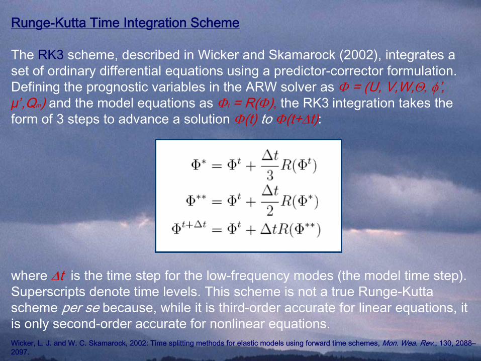
The RK3

scheme, described in Wicker and Skamarock

(2002), integrates a set of ordinary differential equations using a predictor-corrector formulation. Defining the prognostic variables in the ARW solver as Φ = (U, V,W,Θ, φ’, μ’,Qm

) and the model equations as Φt

= R(Φ),

the RK3

integration takes the form of 3 steps to advance a solution Φ(t) to Φ(t+Δt):

where Δt is the time step for the low-frequency modes (the model time step). Superscripts denote time levels. This scheme is not a true Runge-Kutta

scheme per se because, while it is third-order accurate for linear equations, it is only second-order accurate for nonlinear equations.Wicker, L. J. and W. C. Skamarock, 2002: Time splitting methods for elastic models using forward time schemes, Mon. Wea. Rev., 130, 2088–

2097.

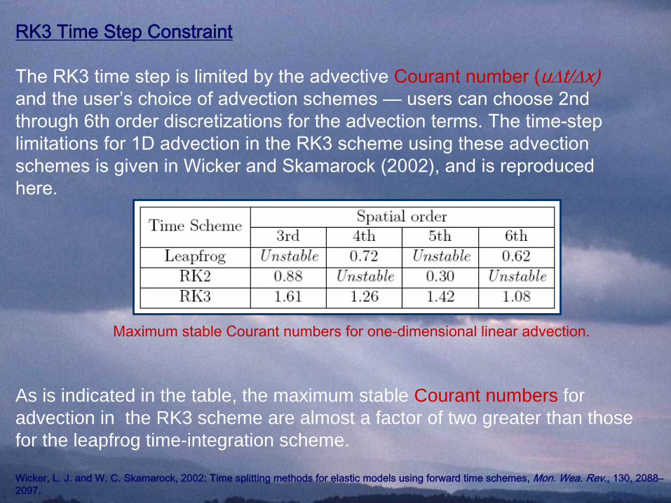
RK3 Time Step Constraint

The RK3 time step is limited by the advective

Courant number (uΔt/Δx) and the user’s choice of advection schemes —

users can choose 2nd through 6th order discretizations

for the advection terms. The time-step limitations for 1D advection in the RK3 scheme using these advection schemes is given in Wicker and Skamarock

(2002), and is reproduced here.

Maximum stable Courant numbers for one-dimensional linear advection.

Wicker, L. J. and W. C. Skamarock, 2002: Time splitting methods for elastic models using forward time schemes, Mon. Wea. Rev., 130, 2088–

2097.

As is indicated in the table, the maximum stable Courant numbers for advection in the RK3 scheme are almost a factor of two greater than those for the leapfrog time-integration scheme.

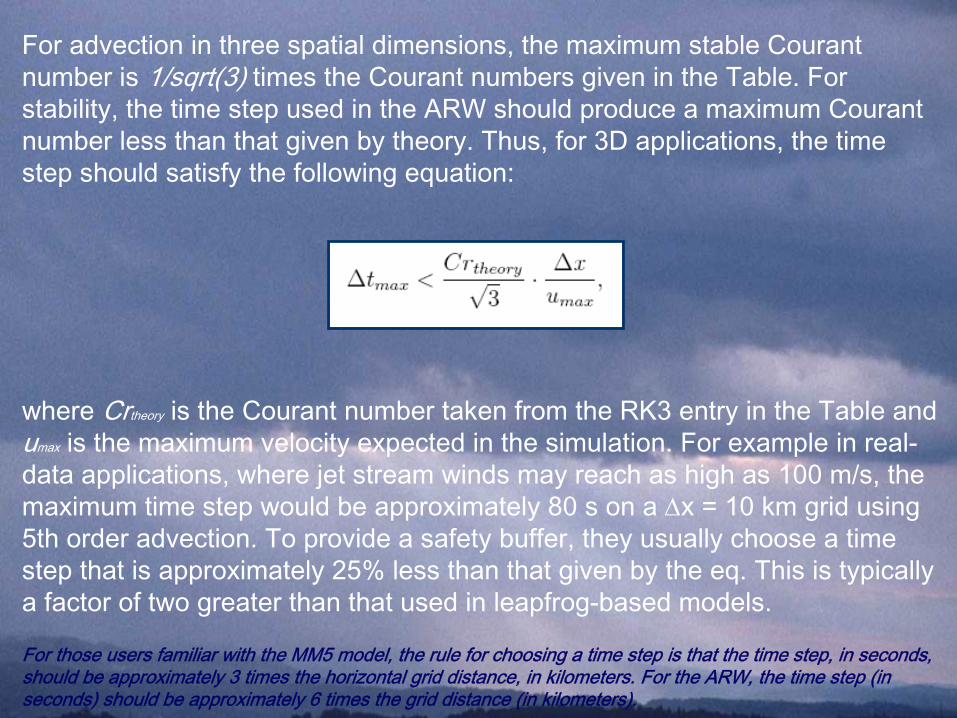
For advection in three spatial dimensions, the maximum stable Courant number is 1/sqrt(3) times the Courant numbers given in the Table. For stability, the time step used in the ARW should produce a maximum Courant number less than that given by theory. Thus, for 3D applications, the time step should satisfy the following equation:

where Crtheory

is the Courant number taken from the RK3 entry in the Table and

umax

is the maximum velocity expected in the simulation. For example

in real-

data applications, where jet stream winds may reach as high as 100 m/s, the maximum time step would be approximately 80 s on a

Δx

= 10 km grid using 5th order advection. To provide a safety buffer, they usually choose a time step that is approximately 25% less than that given by the eq. This is typically a factor of two greater than that used in leapfrog-based models.

For those users familiar with the MM5 model, the rule for choosing a time step is that the time step, in seconds, should be approximately 3 times the horizontal grid distance, in kilometers. For the ARW, the time step (in seconds) should be approximately 6 times the grid distance (in kilometers).

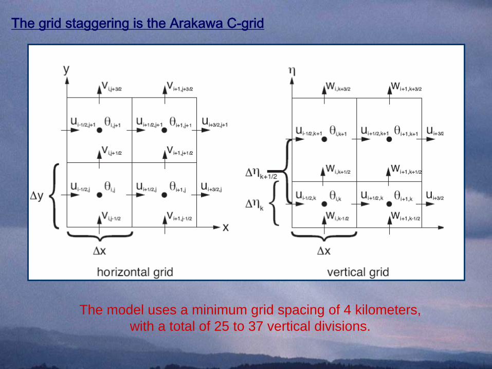
The grid staggering is the Arakawa C-grid

The model uses a minimum grid spacing of 4 kilometers,with a total of 25 to 37 vertical divisions.

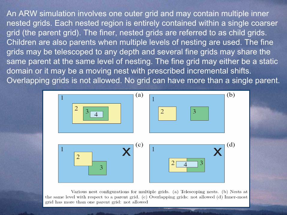
An ARW simulation involves one outer grid and may contain multiple inner nested grids. Each nested region is entirely contained within a single coarser grid (the parent grid). The finer, nested grids are referred to as child grids. Children are also parents when multiple levels of nesting are used. The fine grids may be telescoped to any depth and several fine grids may share the same parent at the same level of nesting. The fine grid may either be a static domain or it may be a moving nest with prescribed incremental shifts. Overlapping grids is not allowed. No grid can have more than a single parent.

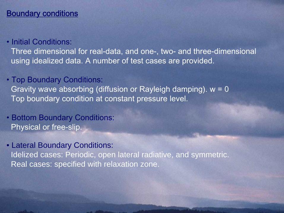
Boundary conditions

• Initial Conditions:Three dimensional for real-data, and one-, two-

and three-dimensionalusing idealized data. A number of test cases are provided.

• Top Boundary Conditions:Gravity wave absorbing (diffusion or Rayleigh damping). w = 0Top boundary condition at constant pressure level.

• Bottom Boundary Conditions:Physical or free-slip.

• Lateral Boundary Conditions:Idelized cases: Periodic, open lateral radiative, and symmetric.Real cases: specified with relaxation zone.

Fine Grid Initialization Options

The ARW supports several strategies to refine a coarse-grid simulation with the introduction of a nested grid. When using 1-way and 2-way nesting, several options for initializing the fine grid are provided.

•

All of the fine grid variables can be interpolated from the coarse grid.

•

All of the fine grid variables can be input from an external file which hashigh-resolution information for both the meteorological and the terrestrialfields.

•

The fine grid can have some of the variables initialized with a high-resolution external data set, while other variables are interpolated from thecoarse grid.

Model Physics

•

Microphysics;

•

Cumulus parameterizations;

•

Surface physics;

•

Planetary boundary layer physics;

•

Atmospheric radiation physics.

Microphysics (mp_physics)

• Kessler scheme:

A warm-rain (i.e. no ice) scheme used commonly inidealized cloud modeling studies (mp_physics

= 1).• Lin et al. scheme:

A sophisticated scheme that has ice, snow and graupel

processes, suitable for real-data high-resolution simulations (2).• WRF Single-Moment 3-class scheme:

A simple efficient scheme withice and snow processes suitable for mesoscale

grid sizes (3).• WRF Single-Moment 5-class scheme:

A slightly more sophisticated version of the previous that allows for mixed-phase processes andsuper-cooled water (4).

• Eta microphysics:

The operational microphysics in NCEP models.A simple efficient scheme with diagnostic mixed-phase processes (5).

• WRF Single-Moment 6-class scheme:

A scheme with ice, snow andgraupel

processes suitable for high-resolution simulations (6).• Thompson et al. scheme:

A new scheme with ice, snow and graupelprocesses suitable for high-resolution simulations (8; replacing theversion in 2.1).

• NCEP 3-class:

An older version of (3) (98).• NCEP 5-class: An older version of (4) (99).

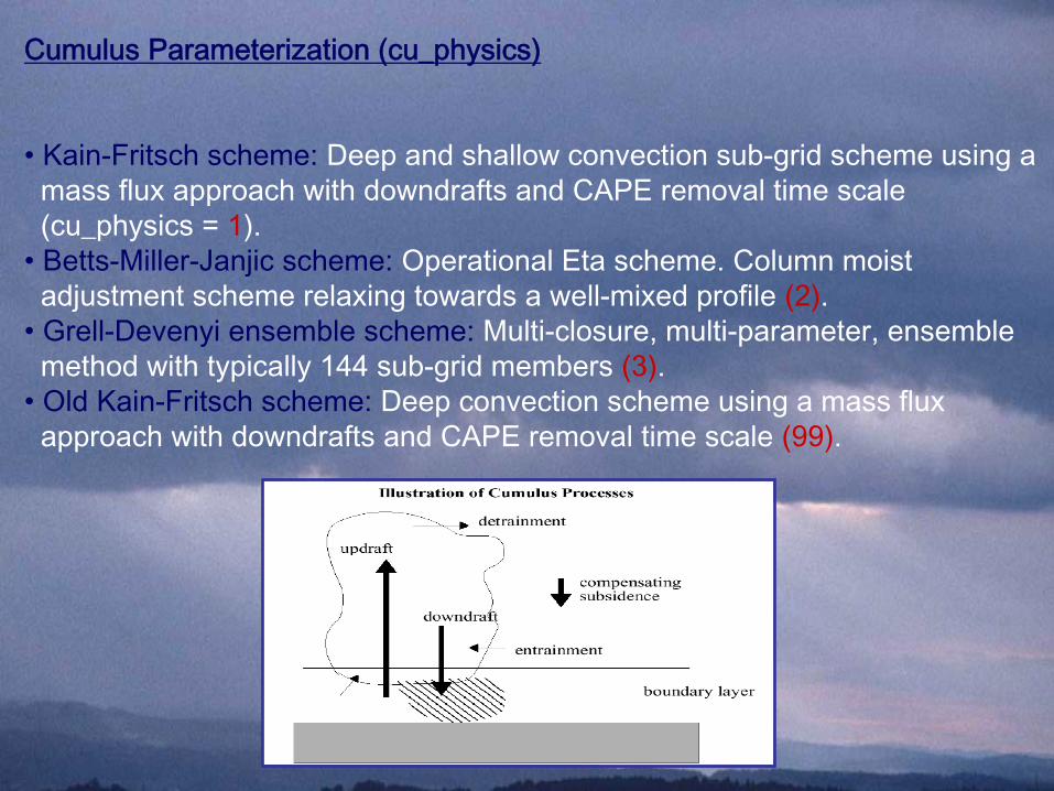
Cumulus Parameterization (cu_physics)

• Kain-Fritsch scheme:

Deep and shallow convection sub-grid scheme using a mass flux approach with downdrafts and CAPE removal time scale(cu_physics

= 1).• Betts-Miller-Janjic

scheme:

Operational Eta scheme. Column moist adjustment scheme relaxing towards a well-mixed profile (2).

• Grell-Devenyi

ensemble scheme:

Multi-closure, multi-parameter, ensemblemethod with typically 144 sub-grid members (3).

• Old Kain-Fritsch scheme:

Deep convection scheme using a mass flux approach with downdrafts and CAPE removal time scale (99).

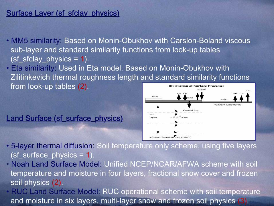
Surface Layer (sf_sfclay_physics)

• MM5 similarity:

Based on Monin-Obukhov

with Carslon-Boland viscoussub-layer and standard similarity functions from look-up tables(sf_sfclay_physics

= 1).• Eta similarity:

Used in Eta model. Based on Monin-Obukhov

with Zilitinkevich

thermal roughness length and standard similarity functionsfrom look-up tables (2).

Land Surface (sf_surface_physics)

• 5-layer thermal diffusion:

Soil temperature only scheme, using five layers(sf_surface_physics

= 1).• Noah Land Surface Model:

Unified NCEP/NCAR/AFWA scheme with soiltemperature and moisture in four layers, fractional snow cover

and frozensoil physics (2).

• RUC Land Surface Model:

RUC operational scheme with soil temperature and moisture in six layers, multi-layer snow and frozen soil physics (3).

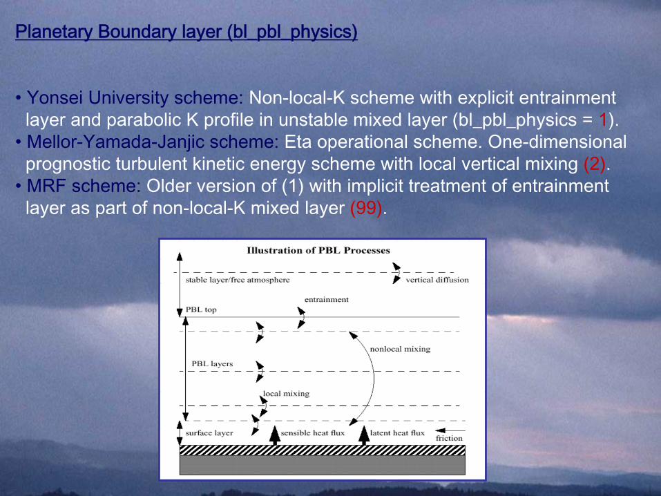
Planetary Boundary layer (bl_pbl_physics)

• Yonsei

University scheme:

Non-local-K scheme with explicit entrainment layer and parabolic K profile in unstable mixed layer (bl_pbl_physics

= 1).• Mellor-Yamada-Janjic

scheme:

Eta operational scheme. One-dimensionalprognostic turbulent kinetic energy scheme with local vertical

mixing (2).• MRF scheme:

Older version of (1) with implicit treatment of entrainmentlayer as part of non-local-K mixed layer (99).

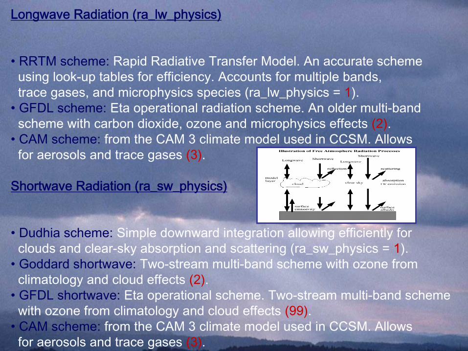
Shortwave Radiation (ra_sw_physics)

• Dudhia

scheme:

Simple downward integration allowing efficiently for clouds and clear-sky absorption and scattering (ra_sw_physics

= 1).• Goddard shortwave:

Two-stream multi-band scheme with ozone fromclimatology and cloud effects (2).

• GFDL shortwave:

Eta operational scheme. Two-stream multi-band schemewith ozone from climatology and cloud effects (99).

• CAM scheme:

from the CAM 3 climate model used in CCSM. Allowsfor aerosols and trace gases (3).

Longwave

Radiation (ra_lw_physics)

• RRTM scheme:

Rapid Radiative

Transfer Model. An accurate schemeusing look-up tables for efficiency. Accounts for multiple bands,trace gases, and microphysics species (ra_lw_physics

= 1).• GFDL scheme:

Eta operational radiation scheme. An older multi-bandscheme with carbon dioxide, ozone and microphysics effects (2).

• CAM scheme:

from the CAM 3 climate model used in CCSM. Allowsfor aerosols and trace gases (3).

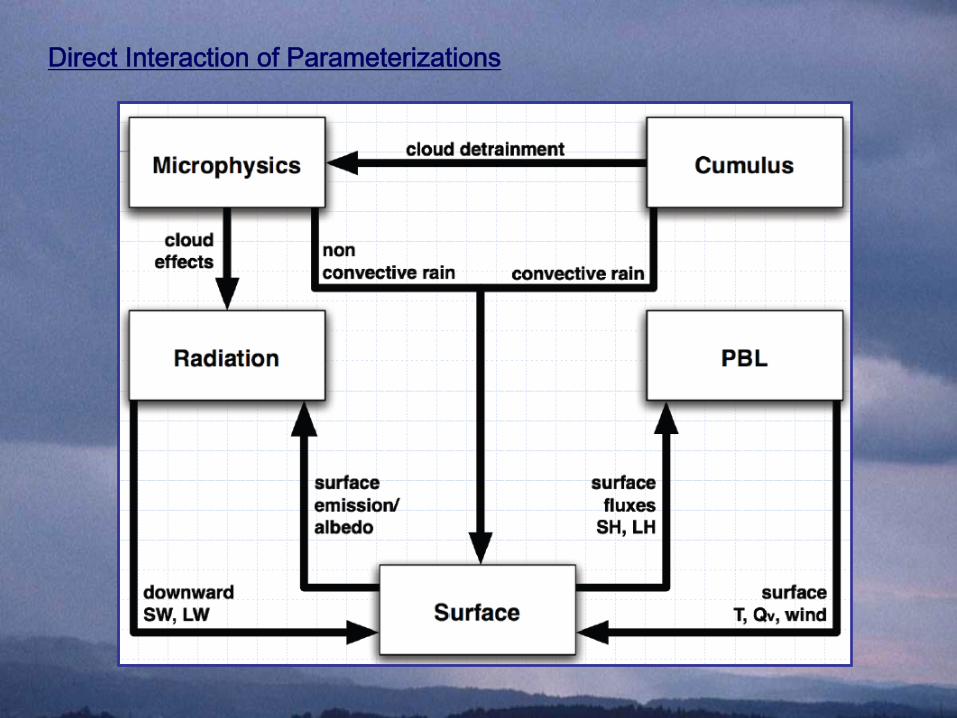
Direct Interaction of Parameterizations

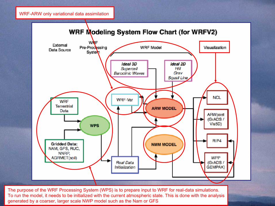
The purpose of the WRF Processing System (WPS) is to prepare input to WRF for real-data simulations.To run the model, it needs to be initialized with the current atmospheric state. This is done with the analysisgenerated by a coarser, larger scale NWP model such as the Nam or GFS

WRF-ARW only variational

data assimilation

References

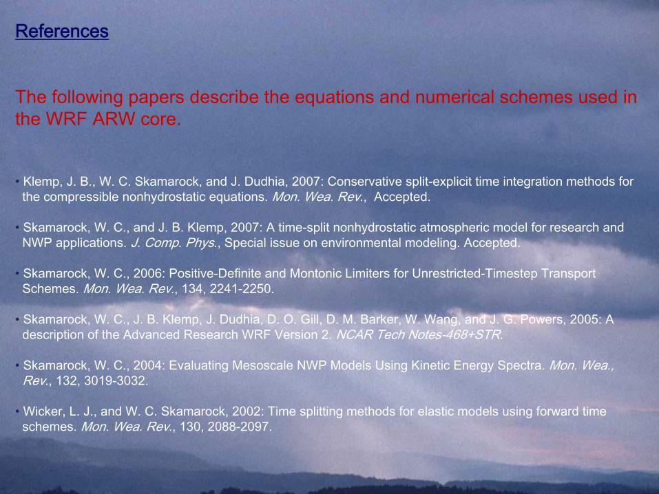
The following papers describe the equations and numerical schemes used in the WRF ARW core.

• Klemp, J. B., W. C. Skamarock, and J. Dudhia, 2007: Conservative split-explicit time integration methods forthe compressible nonhydrostatic

equations. Mon. Wea. Rev., Accepted.

• Skamarock, W. C., and J. B. Klemp, 2007: A time-split nonhydrostatic

atmospheric model for research andNWP applications. J. Comp. Phys., Special issue on environmental modeling. Accepted.

• Skamarock, W. C., 2006: Positive-Definite and Montonic

Limiters for Unrestricted-Timestep

TransportSchemes. Mon. Wea. Rev., 134, 2241-2250.

• Skamarock, W. C., J. B. Klemp, J. Dudhia, D. O. Gill, D. M. Barker, W. Wang, and J. G. Powers, 2005: Adescription of the Advanced Research WRF Version 2. NCAR Tech Notes-468+STR.

• Skamarock, W. C., 2004: Evaluating Mesoscale

NWP Models Using Kinetic Energy Spectra. Mon. Wea.,Rev., 132, 3019-3032.

• Wicker, L. J., and W. C. Skamarock, 2002: Time splitting methods for elastic models using forward timeschemes. Mon. Wea. Rev., 130, 2088-2097.