Descriptor

BIAFLOWS: A Collaborativ

e Framework toReproducibly Deploy and Benchmark BioimageAnalysis Workflows

Highlights

d Image analysis is inescapable in extracting quantitative data

from scientific images

d It can be difficult to deploy and apply state-of-the-art image

analysis methods

d Comparing heterogeneous image analysis methods is

tedious and error prone

d We introduce a platform to deploy and fairly compare image

analysis workflows

Rubens et al., 2020, Patterns 1, 100040June 12, 2020 ª 2020 The Author(s).https://doi.org/10.1016/j.patter.2020.100040

Authors

Ulysse Rubens, Romain Mormont,

Lassi Paavolainen, ...,

Perrine Paul-Gilloteaux,

Rapha€el Maree, Sebastien Tosi

Correspondencesebastien.tosi@irbbarcelona.org

In Brief

While image analysis is becoming

inescapable in the extraction of

quantitative information from scientific

images, it is currently challenging for life

scientists to find, test, and compare

state-of-the-art image analysis methods

compatible with their own microscopy

images. It is also difficult and time

consuming for algorithm developers to

validate and reproducibly share their

methods. BIAFLOWS is a web platform

addressing these needs. It can be used as

a local solution or through an immediately

accessible and curated online instance.

ll

OPEN ACCESS

Please cite this article in press as: Rubens et al., BIAFLOWS: A Collaborative Framework to Reproducibly Deploy and Benchmark Bioimage AnalysisWorkflows, Patterns (2020), https://doi.org/10.1016/j.patter.2020.100040

ll

Descriptor

BIAFLOWS: A Collaborative Frameworkto Reproducibly Deploy and BenchmarkBioimage Analysis WorkflowsUlysse Rubens,1,16 Romain Mormont,1,16 Lassi Paavolainen,2 Volker B€acker,3 Benjamin Pavie,4 Leandro A. Scholz,5

Gino Michiels,6 Martin Ma�ska,7 Devrim Unay,8 Graeme Ball,9 Renaud Hoyoux,10 Remy Vandaele,1 Ofra Golani,11

Stefan G. Stanciu,12 Natasa Sladoje,13 Perrine Paul-Gilloteaux,14 Rapha€el Maree,1,17 and Sebastien Tosi15,17,18,*1Montefiore Institute, University of Liege, 4000 Liege, Belgium2FIMM, HiLIFE, University of Helsinki, 00014 Helsinki, Finland3MRI, BioCampus Montpellier, Montpellier 34094, France4VIB BioImaging Core, 3000 Leuven, Belgium5Universidade Federal do Parana, Curitiba 80060-000, Brazil6HEPL, University of Liege, 4000 Liege, Belgium7Masaryk University, 601 77 Brno, Czech Republic8Faculty of Engineering _Izmir, Demokrasi University, 35330 Balcova, Turkey9Dundee Imaging Facility, School of Life Sciences, University of Dundee, Dundee DD1 5EH, UK10Cytomine SCRL FS, 4000 Liege, Belgium11Life Sciences Core Facilities, Weizmann Institute of Science, Rehovot 7610001, Israel12Politehnica Bucarest, Bucarest 060042, Romania13Uppsala University, P.O. Box 256, 751 05 Uppsala, Sweden14Structure Federative de Recherche Francois Bonamy, Universite de Nantes, CNRS, INSERM, Nantes Cedex 1 13522 44035, France15Institute for Research in Biomedicine, IRB Barcelona, Barcelona Institute of Science and Technology, BIST, 08028 Barcelona, Spain16These authors contributed equally17These authors contributed equally18Lead Contact

*Correspondence: sebastien.tosi@irbbarcelona.org

https://doi.org/10.1016/j.patter.2020.100040

THE BIGGER PICTURE Image analysis is currently one of the major hurdles in the bioimaging chain, espe-cially for large datasets. BIAFLOWS seeds the ground for virtual access to image analysis workflowsrunning in high-performance computing environments. Providing a broader access to state-of-the-art im-age analysis is expected to have a strong impact on research in biology, and in other fields where imageanalysis is a critical step in extracting scientific results from images. BIAFLOWS could also be adoptedas a federated platform to publishmicroscopy images together with theworkflows that were used to extractscientific data from these images. This is a milestone of open science that will help to accelerate scientificprogress by fostering collaborative practices.

Production: Data science output is validated, understood,and regularly used for multiple domains/platforms

SUMMARY

Image analysis is key to extracting quantitative information from scientific microscopy images, but themethods involved are now often so refined that they can no longer be unambiguously described by writtenprotocols. We introduce BIAFLOWS, an open-source web tool enabling to reproducibly deploy and bench-mark bioimage analysis workflows coming from any software ecosystem. A curated instance of BIAFLOWSpopulated with 34 image analysis workflows and 15 microscopy image datasets recapitulating common bio-image analysis problems is available online. The workflows can be launched and assessed remotely bycomparing their performance visually and according to standard benchmark metrics. We illustrated thesefeatures by comparing seven nuclei segmentation workflows, including deep-learning methods. BIAFLOWSenables to benchmark and share bioimage analysis workflows, hence safeguarding research results and

Patterns 1, 100040, June 12, 2020 ª 2020 The Author(s). 1This is an open access article under the CC BY license (http://creativecommons.org/licenses/by/4.0/).

llOPEN ACCESS Descriptor

Please cite this article in press as: Rubens et al., BIAFLOWS: A Collaborative Framework to Reproducibly Deploy and Benchmark Bioimage AnalysisWorkflows, Patterns (2020), https://doi.org/10.1016/j.patter.2020.100040

promoting high-quality standards in image analysis. The platform is thoroughly documented and ready togather annotated microscopy datasets and workflows contributed by the bioimaging community.

INTRODUCTION

As life scientists collect microscopy datasets of increasing size

and complexity,1 computational methods to extract quantita-

tive information from these images have become inescapable.

In turn, modern image analysis methods are becoming so com-

plex (often involving a combination of image-processing steps

and deep-learning methods) that they require expert configura-

tion to run. Unfortunately, the software implementations of

these methods are commonly shared as poorly reusable and

scarcely documented source code and seldom as user-friendly

packages for mainstream bioimage analysis (BIA) platforms.2–4

Even worse, test images are not consistently provided with the

software, and it can hence be difficult to identify the baseline

for valid results or the critical adjustable parameters to optimize

the analysis. Altogether, this does not only impair the reusability

of the methods and impede reproducing published results5,6

but also makes it difficult to adapt these methods to process

similar images. To improve this situation, scientific datasets

are now increasingly made available through public web-based

applications7–9 and open-data initiatives,10 but existing plat-

forms do not systematically offer advanced features such as

the ability to view and process multidimensional images online

or to let users assess the quality of the analysis against a

ground-truth reference (also known as benchmarking). Bench-

marking is at the core of biomedical image analysis challenges

and it a practice known to sustain the continuous improvement

of image analysis methods and promote their wider diffusion.11

Unfortunately, challenges are rather isolated competitions and

they suffer from known limitations12: each event focuses on a

single image analysis problem, and it relies on ad hoc data for-

mats and scripts to compute benchmark metrics. Both chal-

lenge organizers and participants are therefore duplicating ef-

forts from challenge to challenge, whereas participants’

workflows are rarely available in a sustainable and reproducible

fashion. Additionally, the vast majority of challenge datasets

come from medical imaging, not from biology: for instance,

as of January 2020, only 15 out of 198 datasets indexed in

Grand Challenge13 were collected from fluorescence micro-

scopy, one of the most common imaging modalities for

research in biology. As a consequence, efficient BIA methods

are nowadays available but their reproducible deployment

and benchmarking are still stumbling blocks for open science.

In practice, end users are faced with a plethora of BIA ecosys-

tems and workflows to choose from, and they have a hard time

reproducing results, validating their own analysis, or ensuring

that a given method is the most appropriate for the problem

they face. Likewise, developers cannot systematically validate

the performance of their BIA workflows on public datasets or

compare their results to previous work without investing time-

consuming and error-prone reimplementation efforts. Finally,

it is challenging to make BIA workflows available to the whole

scientific community in a configuration-free and reproducible

manner.

2 Patterns 1, 100040, June 12, 2020

RESULTS

Conception of Software Architecture for ReproducibleDeployment and BenchmarkingWithin the Network of European Bioimage Analysts (NEUBIAS

COST [www.cost.eu] Action CA15124), an important body of

work focuses on channeling the efforts of bioimaging stake-

holders (including biologists, bioimage analysts, and software

developers) to ensure a better characterization of existing

bioimage analysis workflows and to bring these tools to a

larger number of scientists. Together, we have envisioned and

implemented BIAFLOWS (Figure 1), a community-driven,

open-source web platform to reproducibly deploy and bench-

mark bioimage analysis workflows on annotated multidimen-

sional microscopy data. Whereas some emerging bioinformatics

web platforms14,15 simply rely on ‘‘Dockerized’’ (https://www.

docker.com/resources/what-container) environments and inter-

active Python notebooks to access and process scientific data

from public repositories, BIAFLOWS offers a versatile and exten-

sible integrated framework to (1) import annotated image data-

sets and organize them into BIA problems, (2) encapsulate BIA

workflows regardless of their target software, (3) batch process

the images, (4) remotely visualize the images together with the

results, and (5) automatically assess the performance of the

workflows from widely accepted benchmark metrics.

BIAFLOWS content can be interactively explored and trig-

gered (Box 1) from a streamlined web interface (Figure 1). For

a given problem, a set of standard benchmark metrics (Supple-

mental Experimental Procedures section 6) are reported for

every workflow run, with accompanying technical and interpre-

tation information available from the interface. One main metric

is also highlighted as the most significant metric to globally

rank the performance of the workflows. To complement bench-

mark results, workflow outputs can also be visualized simulta-

neously from multiple annotation layers or synchronized image

viewers (Figure 2). BIAFLOWS is open-source and thoroughly

documented (https://biaflows-doc.neubias.org/), and extends

Cytomine,16 a web platform originally developed for the collabo-

rative annotation of high-resolution bright-field bioimages. BIA-

FLOWS required extensive software development and content

integration to enable the benchmarking of BIA workflows;

accordingly, the web user interface has been completely rede-

signed to streamline this process (Figure 1). First, a module to

upload multidimensional (C, Z, T) microscopy datasets and a

fully fledged remote image viewer were implemented. Next, the

architecture was refactored to enable the reproducible remote

execution of BIA workflows encapsulated with their original soft-

ware environment in Docker images (workflow images). To ab-

stract out the operations performed by a workflow, we adopted

a rich application description schema17 describing its interface

(input, output, parameters) and default parameter values (Sup-

plemental Experimental Procedures section 3). The system

was also engineered to monitor trusted user spaces hosting a

collection of workflow images and to automatically pull new or

Figure 1. BIAFLOWS Web Interface

(1) Users select a BIA problem (Table S1) and (2) browse the images illustrating this problem, for instance to compare themwith their own images, then (3) select a

workflow (Table S1) and associated parameters (4) to process the images. The results can then be overlaid on the original images from the online image viewer (5),

and (6) benchmark metrics can be browsed, sorted, and filtered both as overall statistics or per image.

llOPEN ACCESSDescriptor

Please cite this article in press as: Rubens et al., BIAFLOWS: A Collaborative Framework to Reproducibly Deploy and Benchmark Bioimage AnalysisWorkflows, Patterns (2020), https://doi.org/10.1016/j.patter.2020.100040

updated workflows (Figure 3, DockerHub). In turn, workflow im-

ages are built and versioned in the cloudwhenever a new release

is triggered from their associated source code repositories (Fig-

ure 3, GitHub). To ensure reproducibility, we enforced that all

versions of the workflow images are permanently stored and

accessible from the system. Importantly, the workflows can be

run on any computational resource, including high-performance

computing and multiple server architectures. This is achieved by

seamlessly converting the workflow images to a compatible

Box 1. How to Get Started with BIAFLOWS

d Watch BIAFLOWS video tutorial (https://biaflows.neubias.o

d Visit BIAFLOWS documentation portal (https://biaflows-doc

d Access BIAFLOWS online instance (https://biaflows.neubias

BIAS (http://neubias.org) and backed by bioimage analysts

BIAFLOWS sandbox server (https://biaflows-sandbox.neub

d Install your own BIAFLOWS instance on a desktop compute

isting BIAFLOWS workflows. Follow ‘‘Installing and populat

d Download a workflow to process your own images locally.

server’’ from the documentation portal.

d Share your thoughts and get help on our forum (https://forum

at biaflows@neubias.org.

format (Singularity18), and dispatching them to the target compu-

tational resources over the network by SLURM19 (Figure 3, addi-

tional computing servers). To enable interoperability between all

components, some standard object annotation formats were

specified for important classes of BIA problems (Supplemental

Experimental Procedures section 4). We also developed a soft-

ware library to compute benchmark metrics associated with

these problem classes by adapting and integrating the code

from existing biomedical challenges13 and scientific

rg).

.neubias.org).

.org) in read-only mode.This public instance is curated by NEU-

and software developers across the world. You can also access

ias.org/) without access restriction.

r or a server to manage images locally or process them with ex-

ing BIAFLOWS locally’’ from the documentation portal.

Follow ‘‘Executing a BIAFLOWS workflow without BIAFLOWS

.image.sc/tags/biaflows), or write directly to our developer team

Patterns 1, 100040, June 12, 2020 3

Figure 2. Synchronizing Image Viewers Displaying Different Workflow Results

Region from one of the sample images available in NUCLEI-SEGMENTATION problem (accessible from the BIAFLOWS online instance). Original image (upper

left), same image overlaid with results from: custom ImageJ macro (upper right), custom CellProfiler pipeline (lower left), and custom Python script (lower right).

llOPEN ACCESS Descriptor

Please cite this article in press as: Rubens et al., BIAFLOWS: A Collaborative Framework to Reproducibly Deploy and Benchmark Bioimage AnalysisWorkflows, Patterns (2020), https://doi.org/10.1016/j.patter.2020.100040

publications.20 With this new design, benchmark metrics are

automatically computed after every workflow run. BIAFLOWS

can also be deployed on a local server to manage private images

and workflows and to process images locally (Figure 3, BIA-

FLOWS local; Supplemental Experimental Procedures section

2). To simplify the coexistence of these different deployment

scenarios, we developed migration tools (Supplementary Exper-

imental Procedures section 5) to transfer content between exist-

ing BIAFLOWS instances (including the online instance

described hereafter). Importantly, all content from any instance

can be accessed programmatically through a RESTful interface,

which ensures complete data accessibility and interoperability.

Finally, for full flexibility, workflows can be downloaded manually

from DockerHub to process local images independently of BIA-

FLOWS (Figure 3, standalone local; Supplemental Experimental

Procedures section 5).

BIAFLOWS Online Curated Instance for PublicBenchmarkingAn online instance of BIAFLOWS is maintained by NEUBIAS and

available at https://biaflows.neubias.org/ (Figure 3). This server

is ready to host community contributions and is already popu-

lated with a substantial collection of annotated image datasets

illustrating common BIA problems and several associated work-

flows to process these images (Table S1). Concretely, we inte-

grated BIAworkflows spanning nine important BIA problem clas-

ses illustrated by 15 image datasets imported from existing

challenges (DIADEM,21 Cell Tracking Challenge,22 Particle

4 Patterns 1, 100040, June 12, 2020

Tracking Challenge,23 Kaggle Data Science Bowl 201824),

created from synthetic data generators25 (CytoPacq,26 TREES

toolbox,27 Vascusynth,28 SIMCEP29), or contributed by

NEUBIAS members.30 The following problem classes are

currently represented: object detection/counting, object seg-

mentation, and pixel classification (Figure 4); particle tracking,

object tracking, filament network tracing, filament tree tracing,

and landmark detection (Figure 5). To demonstrate the versa-

tility of the platform we integrated 34 workflows, each target-

ing a specific software or programming language: ImageJ/FIJI

macros and scripts,31 Icy protocols,32 CellProfiler pipelines,33

Vaa3D plugins,34 ilastik pipelines,35 Octave scripts,36 Jupyter

notebooks,15 and Python scripts leveraging Scikit-learn37 for

supervised learning algorithms, and Keras38 or PyTorch39 for

deep learning. This list, although already extensive, is not

limited, as BIAFLOWS core architecture enables one to seam-

lessly add other software as long as they fulfill minimal require-

ments (Supplemental Experimental Procedures section 3). To

demonstrate the potential of the platform to perform open

benchmarking, a case study has been performed with (and

is available from) BIAFLOWS to compare workflows identifying

nuclei in microscopy images. The content from the BIAFLOWS

online instance (https://biaflows.neubias.org) can be viewed in

read-only mode from the guest account, while the workflows

can be launched from the sandbox server (https://biaflows-

sandbox.neubias.org/). An extensive user guide and video

tutorial are available online from the same URLs. To enhance

their visibility, all workflows hosted in the system are also

Figure 3. BIAFLOWS Architecture and Possible Deployment Scenarios

Workflows are hosted in a trusted source code repository (GitHub). Workflow (Docker) images encapsulate workflows together with their execution environments

to ensure reproducibility. Workflow images are automatically built by a cloud service (DockerHub) whenever a newworkflow is released or an existing workflow is

updated from its trusted GitHub repository. Different BIAFLOWS instances monitor DockerHub and pull new or updated workflow images, which can also be

downloaded to process local images without BIAFLOWS (Standalone Local).

llOPEN ACCESSDescriptor

Please cite this article in press as: Rubens et al., BIAFLOWS: A Collaborative Framework to Reproducibly Deploy and Benchmark Bioimage AnalysisWorkflows, Patterns (2020), https://doi.org/10.1016/j.patter.2020.100040

referenced from NEUBIAS Bioimage Informatics Search Index

(http://biii.eu/). BIAFLOWS online instance is fully extensible

and, with minimal effort, interested developers can package

their own workflows (Supplemental Experimental Procedures

section 3) and make them available for benchmarking (Box

2). Similarly, following our guidelines (Supplemental Experi-

mental Procedures section 2), scientists can make their im-

ages and ground-truth annotations available online through

the online instance or through a local instance they manage

(Box 2). Finally, all online content can be seamlessly migrated

to a local BIAFLOWS instance (Supplemental Experimental

Procedures section 5) for further development or to process

local images.

To further increase the content currently available in

BIAFLOWS online instance, calls for contribution will be shortly

launched to gather more annotated microscopy images and

encourage developers to package their own workflows. The

support of new problem classes is also planned, for example,

to benchmark the detection of blinking events in the context of

super-resolution localization microscopy or the detection of

landmark points for image registration. There is no limitation in

using BIAFLOWS in other fields where image analysis is a critical

step in extracting scientific results from images, for instancema-

terial or plant science and biomedical imaging.

Case Study: Comparing the Performance of NucleiSegmentation by Classical Image Processing, ClassicalMachine Learning, and Deep-Learning MethodsTo illustrate how to useBIAFLOWS for the open benchmarking of

BIA workflows, we integrated seven nuclei segmentation

workflows (Supplemental Experimental Procedures section

1). All content (images, ground-truth annotations, workflows,

benchmark results) is readily accessible from the BIAFLOWS

online instance. The workflows were benchmarked on two

Patterns 1, 100040, June 12, 2020 5

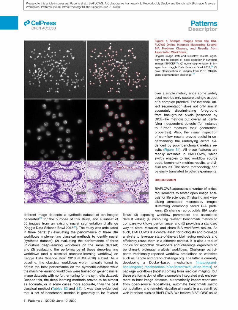
Figure 4. Sample Images from the BIA-

FLOWS Online Instance Illustrating Several

BIA Problem Classes, and Results from

Associated Workflows

Original image (left) and workflow results (right),

from top to bottom: (1) spot detection in synthetic

images (SIMCEP29); (2) nuclei segmentation in im-

ages from Kaggle Data Science Bowl 2018;24 (3)

pixel classification in images from 2015 MICCAI

gland segmentation challenge.40

llOPEN ACCESS Descriptor

Please cite this article in press as: Rubens et al., BIAFLOWS: A Collaborative Framework to Reproducibly Deploy and Benchmark Bioimage AnalysisWorkflows, Patterns (2020), https://doi.org/10.1016/j.patter.2020.100040

different image datasets: a synthetic dataset of ten images

generated29 for the purpose of this study, and a subset of

65 images from an existing nuclei segmentation challenge

(Kaggle Data Science Bowl 201824). The study was articulated

in three parts: (1) evaluating the performance of three BIA

workflows implementing classical methods to identify nuclei

(synthetic dataset); (2) evaluating the performance of three

ubiquitous deep-learning workflows on the same dataset;

and (3) evaluating the performance of these deep-learning

workflows (and a classical machine-learning workflow) on

Kaggle Data Science Bowl 2018 (KDSB2018) subset. As a

baseline, the classical workflows were manually tuned to

obtain the best performance on the synthetic dataset while

the machine-learning workflows were trained on generic nuclei

image datasets with no further tuning for the synthetic dataset.

Despite this, the deep-learning methods proved to be almost

as accurate, or in some cases more accurate, than the best

classical method (Tables S2 and S3). It was also evidenced

that a set of benchmark metrics is generally to be favored

6 Patterns 1, 100040, June 12, 2020

over a single metric, since some widely

used metrics only capture a single aspect

of a complex problem. For instance, ob-

ject segmentation does not only aim at

accurately discriminating foreground

from background pixels (assessed by

DICE-like metrics) but overall at identi-

fying independent objects (for instance

to further measure their geometrical

properties). Also, the visual inspection

of workflow results proved useful in un-

derstanding the underlying errors evi-

denced by poor benchmark metrics re-

sults (Figure S1). All these features are

readily available in BIAFLOWS, which

swiftly enables to link workflow source

code, benchmark metrics results, and vi-

sual results. The same methodology can

be easily translated to other experiments.

DISCUSSION

BIAFLOWS addresses a number of critical

requirements to foster open image anal-

ysis for life sciences: (1) sharing and visu-

alizing annotated microscopy images

illustrating commonly faced BIA prob-

lems; (2) sharing reproducible BIA work-

flows; (3) exposing workflow parameters and associated

default values; (4) computing relevant benchmark metrics to

compare workflows performance; and (5) providing a standard

way to store, visualize, and share BIA workflows results. As

such, BIAFLOWS is a central asset for biologists and bioimage

analysts to leverage state-of-the-art bioimaging methods and

efficiently reuse them in a different context. It is also a tool of

choice for algorithm developers and challenge organizers to

benchmark bioimage analysis workflows. Challenge partici-

pants traditionally reported workflow predictions on websites

such as Kaggle and grand-challenge.org. The latter is currently

developing a Docker-based mechanism (https://grand-

challengeorg.readthedocs.io/en/latest/evaluation.html#) to

package workflows (mostly coming from medical imaging), but

these platforms do not offer a complete integrated web environ-

ment to host image datasets, automatically import workflows

from open-source repositories, automate benchmark metric

computation, and remotely visualize all results in a streamlined

web interface such as BIAFLOWS. We believe BIAFLOWS could

Figure 5. Sample Images from the BIA-

FLOWS Online Instance Illustrating Several

BIA Problem Classes, and Results from

Associated Workflows

Original image (left) and workflow results (right),

from top to bottom: (1) particle tracking in synthetic

time-lapse displaying non-dividing nuclei (Cyto-

PACQ26), single frame + dragon-tail tracks; (2)

neuron tree tracing in 3D image stacks from

DIADEM challenge,21 average intensity projection

(left), traced skeleton z projection (dilated, red); (3)

landmark detection in Drosophila wing images.30

llOPEN ACCESSDescriptor

Please cite this article in press as: Rubens et al., BIAFLOWS: A Collaborative Framework to Reproducibly Deploy and Benchmark Bioimage AnalysisWorkflows, Patterns (2020), https://doi.org/10.1016/j.patter.2020.100040

be made interoperable with the grand-challenge.org Docker-

basedmechanism to packageworkflows, and used by challenge

organizers as a fully integrated platform to automate bench-

marking and share challenge results in a more reproducible

way. Finally, BIAFLOWS provides a solution to authors willing

to share online supporting data,methods, and results associated

with their published scientific results.

With respect to sustainability and scalability, BIAFLOWS is

backed by a team of senior bioimage analysts and software

Box 2. How to Contribute to BIAFLOWS

d Scientists can contribute published annotated microscopy

ground truth annotations and reportedmetrics’’ from the do

ground-truth annotations formats, and contact us through

d To showcase a workflow in the BIAFLOWS online instance,

BIAFLOWS instance or BIAFLOWS sandbox server (https:/

tHub repository: https://github.com/Neubias-WG5/SubmitT

BIAFLOWS instance’’ from the documentation portal.

d Feature requests or bug reports can be posted to BIAFLOW

d Users can contribute to the documentation by submitting a

github.io.

d Any user can share data and results, e.g., accompanying

notebook’’ from the documentation portal or by directly link

developers. The software is compatible with high-performance

computing environments and is based on Cytomine architec-

ture,16 which has already proved itself capable of serving large

datasets to many users simultaneously.41 We invested a large

amount of effort in documenting BIAFLOWS, and the online

instance is ready to receive hundreds of new image datasets

and workflows as community contributions (Box 2). To in-

crease the content of BIAFLOWS online instance, we will

briefly launch calls for contributions targeting existing

images to BIAFLOWS online instance. See ‘‘Problem classes,

cumentation portal for information on the expected images and

the dedicated thread on https://forum.image.sc/tags/biaflows.

developers can encapsulate their source code, test it on a local

/biaflows-sandbox.neubias.org/), and open an issue in this Gi-

oBiaflows. Follow ‘‘Creating a BIA workflow and adding it to a

S GitHub (https://github.com/neubias-wg5).

pull request to https://github.com/Neubias-WG5/neubias-wg5.

scientific publications, via ‘‘Access BIAFLOWS from a Jupyter

ing the content of a BIAFLOWS instance.

Patterns 1, 100040, June 12, 2020 7

llOPEN ACCESS Descriptor

Please cite this article in press as: Rubens et al., BIAFLOWS: A Collaborative Framework to Reproducibly Deploy and Benchmark Bioimage AnalysisWorkflows, Patterns (2020), https://doi.org/10.1016/j.patter.2020.100040

BIAFLOWS problem classes. We propose that BIAFLOWS be-

comes a hub for BIA methods developers, bioimage analysts,

and life scientists to share annotated datasets, reproducible

BIA workflows, and associated results from benchmark and

research studies. In future work, we will work toward interop-

erability with existing European image storage and workflow

management infrastructures such as BioImage Archive,42

https://www.eosc-life.eu/, and Galaxy,15 and further improve

the scalability and sustainability of the platform.

EXPERIMENTAL PROCEDURES

Resource Availability

Lead Contact

Further information and requests for resources should be directed to the Lead

Contact, Sebastien Tosi (sebastien.tosi@irbbarcelona.org).

Materials Availability

No materials were used in this study.

Data and Code Availability

BIAFLOWS is an open-source project and its source code can be freely down-

loaded at https://github.com/Neubias-WG5.

All images and annotations described and used in this article can be down-

loaded from the BIAFLOWS online instance at https://biaflows.neubias.org/.

A sandbox server from which all workflows available in BIAFLOWS online

instance can be launched remotely, and new workflows/datasets appended

for testing are available at https://biaflows-sandbox.neubias.org/.

The documentation to install, use, and extend the software is available at

https://neubias-wg5.github.io/.

SUPPLEMENTAL INFORMATION

Supplemental Information can be found online at https://doi.org/10.1016/j.

patter.2020.100040.

ACKNOWLEDGMENTS

This project is funded by COSTCA15124 (NEUBIAS). BIAFLOWS is developed

by NEUBIAS (http://neubias.org) Workgroup 5, and it would not have been

possible without the great support from the NEUBIAS vibrant community of

bioimage analysts and the dedication of Julien Colombelli and Kota Miura in

organizing this network. Local organizers of the Taggathonswho have fostered

the development of BIAFLOWS are also greatly acknowledged: Chong Zhang,

Gabriel G. Martins, Julia Fernandez-Rodriguez, Peter Horvath, Bertrand Ver-

nay, Aymeric Fouquier d’Herou€el, Andreas Girod, Paula Sampaio, Florian

Levet, and Fabrice Cordelieres. We also thank the software developers who

helped us integrating external code, among others Jean-Yves Tinevez (Image

Analysis Hub of Pasteur Institute) and Anatole Chessel (Ecole Polytechnique).

We thank the Cytomine SCRL FS for developing additional open-source mod-

ules and Martin Jones (Francis Crick Institute) and Pierre Geurts (University of

Liege) for proofreading themanuscript and for their useful comments. R.V. was

supported by ADRIC Pole Mecatech Wallonia grant and U.R. by ADRIC Pole

Mecatech and DeepSport Wallonia grants. R. Maree was supported by an

IDEES grant with the help of theWallonia and the European Regional Develop-

ment Fund. L.P. was supported by the Academy of Finland (grant 310552).

M.M. was supported by the Czech Ministry of Education, Youth and Sports

(project LTC17016). S.G.S. acknowledges the financial support of UEFISCDI

grant PN-III-P1-1.1-TE-2016-2147 (CORIMAG). V.B. and P.P.-G. acknowl-

edge the France-BioImaging infrastructure supported by the French National

Research Agency (ANR-10-INBS-04).

AUTHOR CONTRIBUTIONS

S.T. and R. Maree conceptualized BIAFLOWS, supervised its implementation,

contributed to all technical tasks, and wrote the manuscript. U.R. worked on

the core implementation and web user interface of BIAFLOWS with contribu-

tions from G.M. and R.H. R. Mormont implemented several modules to inter-

8 Patterns 1, 100040, June 12, 2020

face bioimage analysis workflows and the content of the system. S.T., M.M.,

and D.U. implemented the module to compute benchmark metrics. S.T.,

V.B., R. Mormont, L.P., B.P., M.M., R.V., and L.A.S. integrated their own work-

flows or adapted existing workflows, and tested the system. S.T., D.U., O.G.,

and G.B. organized and collected content (image datasets, simulation tools).

S.G.S., N.S., and P.P.-G. provided extensive feedback on BIAFLOWS and

contributed to the manuscript. All authors took part in reviewing the

manuscript.

DECLARATION OF INTERESTS

R Maree and R.H. are co-founders and members of the board of directors of

the non-profit cooperative company Cytomine SCRL FS.

Received: February 14, 2020

Revised: April 4, 2020

Accepted: April 27, 2020

Published: June 3, 2020

REFERENCES

1. Ouyang, W., and Zimmer, C. (2017). The imaging tsunami: computational

opportunities and challenges. Curr. Opin. Syst. Biol. 4, 105–113.

2. Eliceiri, K.W., Berthold, M.R., Goldberg, I.G., Ibanez, L., Manjunath, B.S.,

Martone, M.E., Murphy, R.F., Peng, H., Plant, A.L., Roysam, B., et al.

(2012). Biological imaging software tools. Nat. Methods 9, 697–710.

3. Carpenter, A.E., Kamentsky, L., and Eliceiri, K.W. (2012). A call for bio-

imaging software usability. Nat. Methods 9, 666–670.

4. Schneider, C.A., Rasband, W.S., and Eliceiri, K.W. (2012). NIH Image to

ImageJ: 25 years of image analysis. Nat. Methods 9, 671–675.

5. Munafo, M.R., Nosek, B.A., Bishop, D.V.M., Button, K.S., Chambers, C.D.,

Percie du Sert, N., Simonsohn, U., Wagenmakers, E.-J., Ware, J.J., and

Ioannidis, J.P.A. (2017). A manifesto for reproducible science. Nat. Hum.

Behav. 1, 0021.

6. Hutson, M. (2018). Artificial intelligence faces reproducibility crisis.

Science 359, 725–726.

7. Ellenberg, J., Swedlow, J.R., Barlow, M., Cook, C.E., Sarkans, U.,

Patwardhan, A., Brazma, A., and Birney, E. (2018). A call for public ar-

chives for biological image data. Nat. Methods 15, 849–854.

8. Allan, C., Burel, J.M., Moore, J., Blackburn, C., Linkert, M., Loynton, S.,

Macdonald, D., Moore, W.J., Neves, C., Patterson, A., et al. (2012).

OMERO: flexible, model-driven data management for experimental

biology. Nat. Methods 9, 245–253.

9. Kvilekval, K., Fedorov, D., Obara, B., Singh, A., and Manjunath, B.S.

(2010). Bisque: a platform for bioimage analysis and management.

Bioinformatics 26, 544–552.

10. Williams, E., Moore, J., Li, S.W., Rustici, G., Tarkowska, A., Chessel, A.,

Leo, S., Antal, B., Ferguson, R.K., Sarkans, U., et al. (2017). Image Data

Resource: a bioimage data integration and publication platform. Nat.

Methods 14, 775–781.

11. Vandewalle, P. (2012). Code sharing is associated with research impact in

image processing. Comput. Sci. Eng. 14, 42–47.

12. Maier-Hein, L., Eisenmann, M., Reinke, A., Onogur, S., Stankovic, M.,

Scholz, P., Arbel, T., Bogunovic, H., Bradley, A.P., Carass, A., et al.

(2018). Why rankings of biomedical image analysis competitions should

be interpreted with care. Nat. Commun. 9, 5217.

13. Meijering, E., Carpenter, A., Peng, H., Hamprecht, F.A., and Olivo-Marin,

J.C. (2016). Imagining the future of bioimage analysis. Nat. Biotechnol.

34, 1250–1255.

14. Perkel, J.M. (2018). A toolkit for data transparency takes shape. Nature

560, 513–515.

15. Gr€uning, B.A., Rasche, E., Rebolledo-Jaramillo, B., Eberhard, C.,

Houwaart, T., Chilton, J., Coraor, N., Backofen, R., Taylor, J., and

Nekrutenkoet, A. (2017). Jupyter and Galaxy: easing entry barriers into

llOPEN ACCESSDescriptor

Please cite this article in press as: Rubens et al., BIAFLOWS: A Collaborative Framework to Reproducibly Deploy and Benchmark Bioimage AnalysisWorkflows, Patterns (2020), https://doi.org/10.1016/j.patter.2020.100040

complex data analyses for biomedical researchers. PLoS Comput. Biol.

13, e1005425.

16. Maree, R., Rollus, L., Stevens, B., Hoyoux, R., Louppe, G., Vandaele, R.,

Begon, J.M., Kainz, P., Geurts, P., and Wehenkel, L. (2016).

Collaborative analysis of multi-gigapixel imaging data with Cytomine.

Bioinformatics 32, 1395–1401.

17. Glatard, T., Kiar, G., Aumentado-Armstrong, T., Beck, N., Bellec, P.,

Bernard, R., Bonnet, A., Brown, S.T., Camarasu-Pop, S., Cervenansky,

F., et al. (2018). Boutiques: a flexible framework to integrate command-

line applications in computing platforms. GigaScience 7, giy016.

18. Kurtzer, G.M., Sochat, V., and Bauer, M.W. (2017). Singularity: scientific

containers for mobility of compute. PLoS One 12, e0177459.

19. Yoo, A., Jette, M., and Grondona, M. (2003). SLURM: simple Linux utility

for resource management, job scheduling strategies for parallel process-

ing. Lect. Notes Comput. Sci. 2862, 44–60.

20. Kozubek, M. (2016). Challenges and benchmarks in bioimage analysis.

Adv. Anat. Embryol. Cell Biol. 219, 231–262.

21. Brown, K.M., Barrionuevo, G., Canty, A.J., De Paola, V., Hirsch, J.A.,

Jefferis, G.S., Lu, J., Snippe, M., Sugihara, I., and Ascoli, G.A. (2011).

The DIADEM data sets: representative light microscopy images of

neuronal morphology to advance automation of digital reconstructions.

Neuroinformatics 9, 143–157.

22. Ulman, V., Ma�ska, M., Magnusson, K.E.G., Ronneberger, O., Haubold, C.,

Harder, N., Matula, P., Matula, P., Svoboda, D., Radojevic, M., et al.

(2017). An objective comparison of cell-tracking algorithms. Nat.

Methods 14, 1141–1152.

23. Chenouard, N., Smal, I., de Chaumont, F., Ma�ska, M., Sbalzarini, I.F.,

Gong, Y., Cardinale, J., Carthel, C., Coraluppi, S., Winter, M., et al.

(2014). Objective comparison of particle tracking methods. Nat.

Methods 11, 281–289.

24. Caicedo, J.C., Goodman, A., Karhohs, K.W., Cimini, B.A., Ackerman, J.,

Haghighi, M., Heng, C., Becker, T., Doan, M., McQuin, C., et al. (2019).

Nucleus segmentation across imaging experiments: the 2018 data sci-

ence bowl. Nat. Methods 16, 1247–1253.

25. Svoboda, D., Kozubek, M., and Stejskal, S. (2009). Generation of digital

phantoms of cell nuclei and simulation of image formation in 3D image cy-

tometry. Cytometry A 75, 494–509.

26. Wiesner, D., Svoboda, D., Ma�ska, M., and Kozubek, M. (2019). CytoPacq:

a web-interface for simulating multi-dimensional cell imaging.

Bioinformatics 35, 4531–4533.

27. Cuntz, H., Forstner, F., Borst, A., and H€ausser, M. (2010). One rule to grow

them all: a general theory of neuronal branching and its practical applica-

tion. PLoS Comput. Biol. 6, e1000877.

28. Jassi, P., and Hamarneh, G. (2011). VascuSynth: vascular tree synthesis

software. Insight J http://hdl.handle.net/10380/3260.

29. Lehmussola, A., Ruusuvuori, P., Selinummi, J., Huttunen, H., and Yli-

Harja, O. (2007). Computational framework for simulating fluorescencemi-

croscope images with cell populations. IEEE Trans. Med. Imaging 26,

1010–1016.

30. Vandaele, R., Aceto, J., Muller, M., Peronnet, F., Debat, V., Wang, C.W.,

Huang, C.T., Jodogne, S., Martinive, P., Geurts, P., et al. (2018).

Landmark detection in 2D bioimages for geometric morphometrics: a

multi-resolution tree-based approach. Sci. Rep. 8, 538.

31. Schneider, C.A., Rasband, W.S., and Eliceiri, K.W. (2012). NIH Image to

ImageJ: 25 years of image analysis. Nat. Methods 9, 671–675.

32. de Chaumont, F., Dallongeville, S., Chenouard, N., Herve, N., Pop, S.,

Provoost, T., Meas-Yedid, V., Pankajakshan, P., Lecomte, T., Le

Montagner, Y., et al. (2012). Icy: an open bioimage informatics platform

for extended reproducible research. Nat. Methods 9, 690–696.

33. McQuin, C., Goodman, A., Chernyshev, V., Kamentsky, L., Cimini, B.A.,

Karhohs, K.W., Doan, M., Ding, L., Rafelski, S.M., Thirstrup, D., et al.

(2018). CellProfiler 3.0: next-generation image processing for biology.

PLoS Biol. 16, e2005970.

34. Peng, H., Ruan, Z., Long, F., Simpson, J.H., and Myers, E.W. (2010). V3D

enables real-time 3D visualization and quantitative analysis of large-scale

biological image data sets. Nat. Biotechnol. 28, 348–353.

35. Berg, S., Kutra, D., Kroeger, T., Straehle, C.N., Kausler, B.X., Haubold, C.,

Schiegg, M., Ales, J., Beier, T., Rudy, M., et al. (2019). ilastik: interactive

machine learning for (bio)image analysis. Nat. Methods 16, 1226–1232.

36. Eaton, J.W., Bateman, D., Hauberg, S., and Wehbring, R. (2016). GNU

Octave Version 4.2.0 Manual: A High-Level Interactive Language for

Numerical Computations (Free Software Foundation). https://octave.org/

doc/octave-4.2.0.pdf.

37. Pedregosa, F., Varoquaux, G., Gramfort, A., Michel, V., Thirion, B., Grisel,

O., Blondel, M., Prettenhofer, P., Weiss, R., Dubourg, V., et al. (2011).

Scikit-learn: machine learning in Python. J. Mach. Learn. Res. 12,

2825–2830.

38. Chollet, F. (2017). Deep Learning with Python (Manning).

39. Paszke, A., Gross, S., Chintala, S., Chanan, G., Yang, E., DeVito, Z., Lin, Z.,

Desmaison, A., Antiga, L., Lerer, A. (2017). Automatic Differentiation in

PyTorch. NIPS Autodiff Workshop, 2017.

40. Sirinukunwattana, K., Pluim, J.P.W., Chen, H., Qi, X., Heng, P.A., Guo,

Y.B., Wang, L.Y., Matuszewski, B.J., Bruni, E., Sanchez, U., et al.

(2017). Gland segmentation in colon histology images: the glas challenge

contest. Med. Image Anal. 35, 489–502.

41. Multon, S., Pesesse, L., Weatherspoon, A., Florquin, S., Van de Poel, J.F.,

Martin, P., Vincke, G., Hoyoux, R., Maree, R., Verpoorten, D., et al. (2018).

A Massive Open Online Course (MOOC) on practical histology: a goal, a

tool, a large public! Return on a first experience. Ann. Pathol. 38, 76–84.

42. Ellenberg, J., Swedlow, J.R., Barlow, M., Cook, C.E., Sarkans, U.,

Patwardhan, A., Brazma, A., and Birney, E. (2018). A call for public ar-

chives for biological image data. Nat. Methods 15, 849–854.

Patterns 1, 100040, June 12, 2020 9

PATTER, Volume 1

Supplemental Information

BIAFLOWS: A Collaborative Framework

to Reproducibly Deploy and Benchmark

Bioimage Analysis Workflows

Ulysse Rubens, Romain Mormont, Lassi Paavolainen, Volker Bäcker, BenjaminPavie, Leandro A. Scholz, Gino Michiels, Martin Ma�ska, Devrim Ünay, GraemeBall, Renaud Hoyoux, Rémy Vandaele, Ofra Golani, Stefan G. Stanciu, NatasaSladoje, Perrine Paul-Gilloteaux, Raphaël Marée, and Sébastien Tosi

Problem class Problem Workflow repository BISE link

1. Object detection SPOT-COUNTING-2DW_SpotDetection-IJ

http://biii.eu/spot-detection-imagej

/ SPOT-DETECTION-2D W_SpotDetection-Icy http://biii.eu/spot-detection-icy

2. Object counting W_SpotDetection-Dmap-IJ http://biii.eu/node/1603

SPOT-COUNTING-3D W_SpotDetection3D-IJ http://biii.eu/node/1458

SPOT-DETECTION-3D W_SpotDetection3D-Icy http://biii.eu/node/1604

W_SpotDetection3D-Hessian-IJ

http://biii.eu/spot-detection-3d-

hessian-imagej

3. Object

segmentation

NUCLEI-

SEGMENTATION W_NucleiSegmentation-ImageJ

http://biii.eu/nuclei-segmentation-

2d-imagej

W_NucleiSegmentation-CellProfiler

https://biii.eu/nuclei-segmentation-

cellprofiler

W_NucleiSegmentation-Python

http://biii.eu/nuclei-segmentation-

python

W_NucleiSegmentation-MaskRCNN https://biii.eu/node/1487

W_NucleiSegmentation-DeepCell http://biii.eu/node/1607

W_NucleiSegmentation-UNet http://biii.eu/node/1608DATA-SCIENCE-

BOWL-2018 W_NucleiSegmentation-MaskRCNN https://biii.eu/node/1487

W_NucleiSegmentation-UNet http://biii.eu/node/1608

W_NucleiSegmentation-ilastik

https://biii.eu/nuclei-segmentation-

ilastik

NUCLEI-

SEGMENTATION-3D W_NucleiSegmentation3D-ImageJ

http://biii.eu/nuclei-segmentation-

3d-imagej

W_NucSeg3DThr-ImageJ http://biii.eu/node/1609

W_NucleiSegmentation3D-ilastik http://biii.eu/node/1610

4. Pixel classificationGLAND-

SEGMENTATION W_PixCla-UNet-GlaS

https://biii.eu/pixel-classification-

glas-challenge-unet

5. Particle trackingNUCLEI-TRACKING-

NODIVISION W_NucleiTracking-ImageJ

https://biii.eu/nuclei-tracking-

imagej

W_LogPartTrack_IJ http://biii.eu/node/1611

W_NucleiTrackingTrackmate-IJ

http://biii.eu/nuclei-tracking-

trackmate

W_ObjectTracking-Octave http://biii.eu/node/1615

W_ObjectTraking-MU-Lux-CZ http://biii.eu/node/1616NUCLEI-TRACKING-

3D NO WORKFLOW YET

6. Object trackingNUCLEI-TRACKING-

DIVISIONW_ObjectTracking-ImageJ http://biii.eu/node/1614

Table S1. BIA problems and workflows currently available from BIAFLOWS online instance. Related to Figure 1. Problem class: type of image analysis problem. Problem: concrete BIA problem, as listed from BIAFLOWS > Problems webpage. Workflows repository: code repository, as linked from BIAFLOWS > Workflows webpage (and stored at https://github.com/Neubias-WG5). BISE link: workflow webpage on BISE, NEUBIAS Bioimage Informatics Search Engine.

7. Filament tree

network tracingNEURON-TRACING-3D W_NeuronTracing_vaa3d https://biii.eu/app-all-path-pruning

W_NeuronTracing_vaa3d_app2 http://biii.eu/node/1617

W_NeuronTracing3D_Rivuletpy http://biii.eu/node/1618

W_NeuronTracing_vaa3d_most http://biii.eu/node/1620

W_NeuronTracing_vaa3d_fastmarching_spanningtreehttp://biii.eu/node/1623NEURON-TRACING-

TREES-3DW_NeuronTracing_vaa3d https://biii.eu/app-all-path-pruning

W_NeuronTracing_vaa3d_app2 http://biii.eu/node/1617

W_NeuronTracing_vaa3d_most http://biii.eu/node/1620

W_NeuronTracing_vaa3d_fastmarching_spanningtreehttp://biii.eu/node/16238. Filament network

tracingVESSEL-TRACING-3D W_FilamentTracing3D-ImageJ http://biii.eu/node/1453

W_FilamentTracing3D-Tub-IJ http://biii.eu/node/1621

W_FilamentTracing3D-LocThr-IJ http://biii.eu/node/1622

W_LandmarkDetect-ML-MSET-Predhttps://biii.eu/landmark-detection-

mset-models-prediction

W_LandmarkDetect-ML-LC-Predhttps://biii.eu/landmark-detection-

lc-models-prediction

W_LandmarkDetect-ML-DMBL-Pred https://biii.eu/node/1485

9. Landmark

detectionLANDMARKS-DROSO

Name mAP FO DICE AHD

w_nucleisegmentation_maskrcnn 0.606 0.797 0.915 0.224

w_nucleisegmentation_unet 0.596 0.795 0.922 0.361

w_nucleisegmentation-imagej 0.593 0.821 0.912 0.119

w_nucleisegmentation_deepcell 0.58 0.768 0.917 0.416

w_nucleisegmentation-python 0.549 0.763 0.904 0.322

w_nucleisegmentation_cellprofiler 0.482 0.724 0.872 0.148

Table S2. Benchmark metrics results for the six nuclei segmentation workflows (SIMCEP dataset). Best results in bold, green highlights results significantly better than average, and red highlights results significantly worse than average.

Name mAP FO DICE AHD

w_nucleisegmentation_maskrcnn 0.394 0.625 0.798 2.702

w_nucleisegmentation_unet 0.282 0.542 0.754 8.485

w_nucleisegmentation_ilastik 0.208 0.502 0.725 3.843

Table S3. Benchmark metrics results for the three nuclei segmentation machine learning workflows (DSB dataset). Best results in bold, green highlights results significantly better than average, and red highlights results significantly worse than average.

Figure S1. Some workflow results (SIMCEP dataset). Cropped out regions from original images (left), same regions with workflow results overlay (right), top: U-NET (red) and CellProfiler (orange), bottom: DeepCell (green) and CellProfiler (orange).

Supplemental Experimental Procedures

Section 1. Case study: Nuclei segmentation

In this section, we present two simple comparison experiments showcasing BIAFLOWS features. Both experiments can be fully reproduced from BIAFLOWS online instance. Datasets (available from BIAFLOWS > Problems)

1. BIAFLOWS NUCLEI-SEGMENTATION (SIMCEP), Related to Figure 2 10 synthetic grayscale images simulating widefield fluorescence microscopy images created by

1. The images exhibit strong non-uniform illumination, saturation, and some nuclei are

heavily clustered.

2. BIAFLOWS DATA-SCIENCE-BOWL-2018 (DSB), Related to Figure 4 65 RGB images from Data Science Bowl 2018 challenge dataset

2, exhibiting heterogeneous

stained nuclei samples imaged from various microscopy modalities. Workflows (available from BIAFLOWS > Workflows), Related to Figure 2 and Figure S1

Name Pre-processing

Classification Mask post-processing

w_nucleisegmentation-imagej

Laplacian of Gaussian

Global threshold (user defined)

Binary watershed from distance map

w_nucleisegmentation-python

Gaussian blur

Adaptive threshold (local mean)

Binary watershed from smoothed distance map, remove small objects

w_nucleisegmentation_cellprofiler

Illumination correction

Global threshold (3 class Otsu’s method)

Hole filling, Binary watershed from smoothed distance map, remove small and large objects

w_nucleisegmentation_ilastik

None 2 class pixel random forest classifier

1 (trained

on 15 images from DSB2018 training set 1)

Hole filling, binary watershed from smoothed distance map, remove small objects

w_nucleisegmentation_maskrcnn

3

None Pre-trained Mask R-CNN model from

4 (trained on

670 images from DSB2018 training set 1)

None, but classifier accounts for object geometry

w_nucleisegmentation_unet

5

None 3 class pixel classifier U-NET model trained

2 on

670 images from DSB2018 training set 1

Hole filling, binary watershed from smoothed distance map, remove small and edge touching objects

w_nucleisegmentation_deepcell

None Pre-trained DeepCell 1.0 model from

6 (trained on

mammalian nuclei images)

Hole filling, binary watershed from smoothed distance map, remove small and edge touching objects

1 Features: Gaussian Smoothing, Laplacian of Gaussian, Gaussian Gradient Magnitude, Difference of

Gaussians, Structure Tensor Eigenvalues, Hessian of Gaussian Eigenvalues. Sigma: 0.7, 1.0, 1.6 and 3.5. 2 lr = 1e-4, 15 epochs (500 steps), batch size: 10, loss: weighted cross-entropy, optimizer: RMSprop.

Benchmark metrics (reported in BIAFLOWS > Problems > Workflow runs), Related to Figure 1 Dice coefficient (DICE, 0-1): normalized overlap between ground truth and prediction binary masks. DICE is equal to 1 only for perfect segmentation. Average Hausdorff Distance (AHD, >=0): average distance between object pixels in ground truth (/prediction) masks and closest object pixels in prediction (/ground truth) masks. AHD is equal to 0 only for perfect segmentation. Fraction overlap (FO, 0-1): 0.5 fraction overlap can be interpreted as "on average the overlap of a predicted object with the ground truth object with largest overlap is half the area of the larger of these two objects". This would for instance happen if objects are either systematically split into two identical objects or merged by pair. FO is equal to 1 only for perfect segmentation. Mean Average Precision (mAP, 0-1)

2: IoU (Intersection over Union) between predicted and

ground-truth objects are computed. IoU are then compared to 10 thresholds (0.5, 0.55 ... 0.95) and, if greater, the object is set as true positive (TP) for that threshold. Precision is computed as P = TP / (TP + FP + FN) for each threshold, where FP = number of predicted objects - TP and FN = number of ground-truth objects - TP. Precision is finally averaged out for all objects and images. mAP is equal to 1 only for perfect segmentation.

Benchmark metrics results (available from BIAFLOWS > Problems > Workflow runs) Synthetic nuclei image dataset (SIMCEP) The aim of this first experiment is two-fold: 1) comparing the performance of three nuclei segmentation workflows implementing classical image analysis methods, and which parameters were manually tuned for the SIMCEP dataset, 2) comparing the performance of these workflows to three Deep Learning (DL) workflows trained on generic nuclei microscopy image datasets. All content, including workflow source code, workflows parameters used for this experiment, benchmark metrics results, and workflow visual results, are available online: https://biaflows.neubias.org/#/project/5955/analysis. The benchmark metrics results of this experiment are summarized in Table S2. For object segmentation, mean Average Precision (mAP, from Data Science Bowl 2018 challenge) is one of the most relevant metric (main metric) since it assesses the ability of a workflow to identify independent nuclei. Despite the fact that they were trained on generic nuclei datasets, DL workflows achieve among the best mAP. Clearly, DICE and AHD only reflects one aspect of the problem, concretely the ability of a workflow to classify pixels as being part of an object (DICE coefficient), or in its vicinity (Average Hausdorff Distance, AHD). As a consequence, DICE metric is poorly discriminative for this experiment as it does not account for erroneous object merging or splitting. Still, comparing the best (U-NET) and worse workflow (CellProfiler) for DICE metric, it is apparent that this latter tend to overestimate the extension of the nuclei by including part of the blur surrounding them. AHD is rather poorly informative for this experiment, the only two workflows achieving significantly higher AHD are the only ones excluding nuclei touching the edges (these objects contribute to significantly increasing AHD). A simple workflow consisting of Laplacian of Gaussian (LoG) pre-filtering followed by user defined global thresholding (ImageJ workflow) and binary watershed achieves close or better than the DL workflows, and it is the most successful classical method represented. This is probably since 1) the size of the nuclei is rather uniform for this dataset (LoG radius can be fine-tuned), 2) the images suffer from heavy non-uniform illumination (LoG is insensitive to smooth intensity variations) and 3) some nuclei are heavily clustered (LoG displays a strong response around blobs helping to split them apart). Fine-tuned local adaptive thresholding (Python workflow) and illumination correction followed by automatic global thresholding (CellProfiler workflow), both followed by similar post-processing, achieve lower mAP. CellProfiler workflow especially does not manage to identify independent nuclei in heavily clustered regions. Finally, the results from the relatively simpler Fraction Overlap (FO) metric (implemented for the first time in BIAFLOWS) correlates quite well with the more complex mAP metric results.

Real microscopy nuclei dataset (DSB) The aim of this experiment is two-fold: 1) comparing some of the previous deep learning workflows on a real microscopy test set similar to their training sets, 2) comparing their performance to a more classical machine learning workflow (Ilastik, using local feature extraction and random forest pixel classification). All content, including workflow source code, workflows parameters used for this experiment, benchmark metrics results, and workflow visual results, are available online: https://biaflows.neubias.org/ #/project/12182234/analysis. The benchmark metrics results of this experiment are summarized in Table S3. Overall, all metric results are significantly worse than for the previous experiment, showing that this dataset is far more challenging. Due to the complexity and heterogeneity of this dataset, classical workflows were not evaluated. DeepCell 1.0 workflow was also excluded since it was trained on a dataset too different from DSB dataset (grayscale, fluorescence microscopy images). Mask R-CNN clearly outperforms other ML workflows (for all four metrics), suggesting that a strategy consisting in classifying pixels and splitting apart clusters of objects is not as successful as direct object detection and segmentation for complex images. It is also apparent that more classical pixel classification ML techniques (Ilastik) are not able to deal with class heterogeneity as well as DL methods. As a common practice, Ilastik developers actually recommend to enforce in class homogeneity, which cannot be checked for this dataset. Also, Ilastik was only trained from 15 representative images of the whole training set (65 images) since the size of the model quickly becomes unpractical for growing image numbers (the software is originally designed for sparse hand annotations). Discussion This simple case study showcased some important BIAFLOWS features and the importance of using a set of benchmark metrics (as opposed to a single metric). It also confirmed the versatility of Deep Learning methods, both to deal with heterogeneous datasets

2, and to generalize to datasets

completely different than their training sets (even without transfer learning or other advanced strategies). The simple Fraction Overlap (FO) metric that we implemented for BIAFLOWS correlates quite well with the more complex mean Average Precision (mAP) proposed for the Data Science Bowl challenge. These two metrics are undoubtedly the best of the four metrics to capture the ability of the workflows to identify independent objects. mAP metric seems slightly more sensitive than the simpler FO metric, but this latter is easier to interpret in terms of the average normalized overlap between predicted and ground truth objects. DICE and AHD metrics, while bringing complementary information and orientation on how to interpret difference in performance, are not sufficient to assess true accuracy since they do not account for object splitting and merging errors. Importantly, visual inspection was instrumental to conclude on the actual shortcomings of the workflows. BIAFLOWS enables to browse benchmark metrics results both as agglomerated statistics and per image, and it is also easy to jump from benchmark metrics results to the original images or compare visual workflow results side by side. Finally, all results are publically available (including workflows source code) and can be reproduced online, which contrasts with common benchmarking publication practices, e.g.

2, where the code provided sometimes requires expert setup to run locally.

BIAFLOWS workflow runs for SIMCEP dataset. For every run, the parameters used and the execution log can be retrieved from drop down tabs.

BIAFLOWS workflow metric results table for the SIMCEP dataset. Top: aggregated (all images, metrics average and standard deviation), bottom: metrics per image.

BIAFLOWS gallery showing cells segmented by U-NET (first 25) from DSB dataset. Each individual object can be clicked and visualized in context.

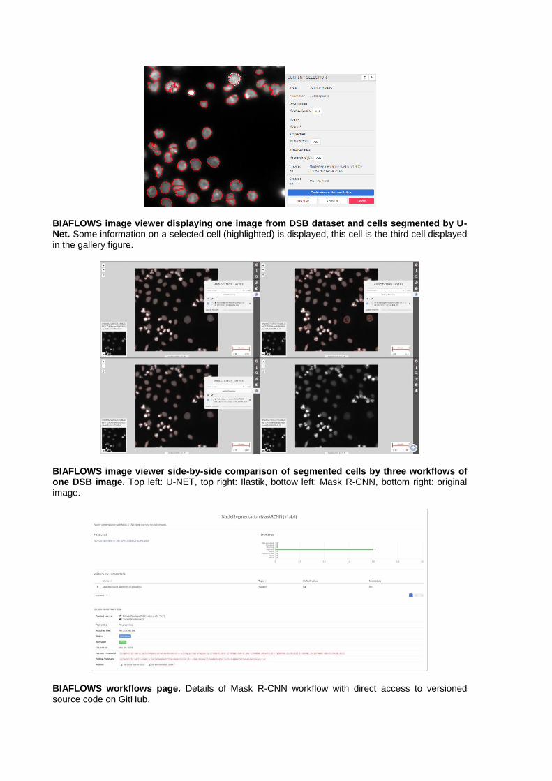
BIAFLOWS image viewer displaying one image from DSB dataset and cells segmented by U-Net. Some information on a selected cell (highlighted) is displayed, this cell is the third cell displayed in the gallery figure.

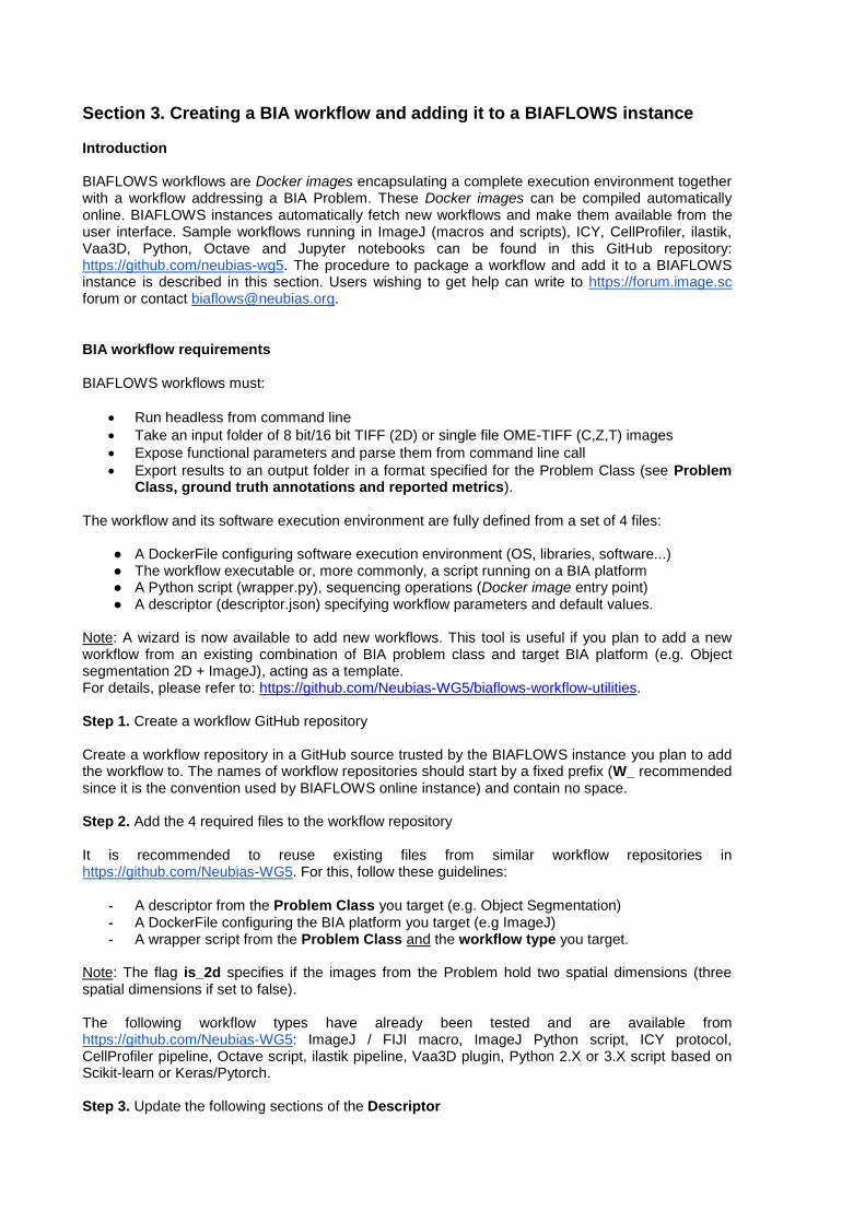
BIAFLOWS image viewer side-by-side comparison of segmented cells by three workflows of one DSB image. Top left: U-NET, top right: Ilastik, bottow left: Mask R-CNN, bottom right: original image.

BIAFLOWS workflows page. Details of Mask R-CNN workflow with direct access to versioned source code on GitHub.

Section 2. Installing and populating BIAFLOWS locally

It is possible to install BIAFLOWS on a local server or a desktop computer. This might be useful to manage and analyse images locally or organize challenges. The procedure is described below and should take less than 30 minutes (UNIX-like based system recommended). Installing a local instance of BIAFLOWS The procedure described in this section is for Linux Ubuntu but it should be possible to install BIAFLOWS on other platforms (not tested). Some specific details related to deployment on Mac OS can be found online: https://doc.uliege.cytomine.org/display/PubOp/Install+Cytomine+on+MacOS 1/ Installation requirements BIAFLOWS runs in Docker containers, the only requirement is to install Docker. Check the official Docker documentation to install Docker for Ubuntu: https://docs.docker.com/install/linux/docker-ce/ubuntu/ Choose Install using the repository, set up the repository and install Docker CE. 2/ Retrieve BIAFLOWS installation files by typing the following commands in a terminal mkdir Biaflows/ cd Biaflows/ git clone https://github.com/Neubias-WG5/Biaflows-bootstrap.git cd Biaflows-bootstrap 3/ Configure the local instance Edit configuration.sh and, if necessary, update URLs (CORE_URL, IMS_URL, UPLOAD_URL). Make sure to use URLs that are not already used by other applications (avoid localhost) to prevent conflicts. In /etc/hosts of the host machine, add the following lines, adapting them accordingly to chosen XXX_URL in configuration.sh. 127.0.0.1 biaflows

127.0.0.1 biaflows-ims

127.0.0.1 biaflows-upload

127.0.0.1 rabbitmq

If needed, update data path variables (IMS_STORAGE_PATH…) in configuration.sh. All data paths must be valid and mappable in the Docker engine. If they don't exist, create the directories (mkdir) corresponding to the following variables: A reference to these URLs and paths is provided here: https://doc.uliege.cytomine.org/display/PubOp/Cytomine+configuration+reference Configure BIAFLOWS_WORKFLOWS_METRICS to true or false depending if you want to perform benchmarking or not on this instance: ground truth annotations are then required for all images. Set this flag to false if you plan to manage / process local images only. 4/ Initialize the deployment Run the installation script: sudo bash init.sh 5/ Deploy the local instance Run the generated deployment script: sudo bash start.sh 6/ Check the running instance

When startup is finished, check that the application is running in your browser at the URL specified by CORE_URL (default: http://biaflows). Three accounts with different access rights are automatically created (username: admin; password: admin; username: guest; password: guest; username: neubias; password: neubias). Passwords should be updated from the Account page (top right). 7/ Install sample Problems (images and ground-truth data) After BIAFLOWS is successfully installed locally, the local instance is empty. All projects available in BIAFLOWS online instance can be imported to the local instance. For this, get the public and private keys of the admin account (Account page), then run: cd Biaflows-bootstrap sudo bash ./inject_demo_data.sh ADMIN_PUBLIC_KEY ADMIN_PRIVATE_KEY where ADMIN_PUBLIC_KEY and ADMIN_PRIVATE_KEY have been substituted with their respective values. The script starts to download projects and import them in your local BIAFLOWS. The list of imported projects can be tweaked by editing the file Biaflows-bootstrap/configs/project_migrator/projects.txt. The whole data injection procedure can take several minutes, depending on your Internet connection and the number of projects being imported. Creating a new Problem (project) in a local BIAFLOWS instance To create a new problem, connect as regular user or admin. 1/ Go to the Problems tab

2/ Click New Problem

3/ Choose a meaningful problem name and save

4/ The problem is ready to be configured, the following configuration is recommended

5/ Assign your problem to a problem class (see Section 4 Problem Class, Ground truth annotations and reported metrics) by clicking on Change problem class. The problem class specifies the format of ground truth annotations (and workflow outputs), as well as the associated benchmark metrics to be computed (if benchmark is enabled).

6/ Configure project members. If you work alone, you can leave contributors and project managers to default user. This can be done from the “Members” tab in the problem configuration. 7/ The problem can be fully configured to display or hide panels / tabs / tools in the user interface. This is achieved from the Custom UI tab in the problem configuration. 8/ A description of the problem can optionally be added from the Information (left sidebar). The description is displayed in Problems list. Uploading images to a local BIAFLOWS instance To upload new images, connect as regular user or admin. Supported formats

- 2D images: 8-bit/16-bit TIFF (or OME-TIFF files) - Multi-dimensional images (Z, C, T): single file 8-bit/16-bit OME-TIFF

Note: The text string _lbl should not be used in image names since it is a reserved string for ground truth annotation images. 1/ Go to Storage section

2/ Select the Problem to which the images should be associated with (Link with problem)

Note: If a problem is not in the list, make sure you are a member for this problem 3/ Click on Add files… and select the files from the file browser 4/ Start upload with Start upload and wait until completion The status can be:

DEPLOYED/CONVERTED: The image is correctly imported to BIAFLOWS ERROR FORMAT: The file format is not supported ERROR EXTRACTION: Something went wrong during metadata extraction ERROR CONVERSION: Something went wrong during the conversion of the image into the

BIAFLOWS internal image format ERROR DEPLOYMENT: Something went wrong during the communication with BIAFLOWS

API. It can be due to access rights, or other unexpected error Note: Images uploaded to storage can also be associated to a Problem after upload (Problem: Add image). This can be useful to associate the same image to several Problems. Uploading ground truth annotations to an existing BIAFLOWS problem If you plan to perform benchmarking, ground truth annotations should also be uploaded and associated to every image of a problem. The format of these annotations depends on the associated problem class (see Section 4 Problem Class, ground truth annotations and reported metrics). Image annotations (e.g. binary masks) should be uploaded as 16-bit TIFF (or OME-TIFF) for 2D images and as single file 16-bit OME-TIFF for multidimensional (C,Z,T) images. They should be uploaded by following the procedure described in the previous section and by setting the same name as their corresponding image + _lbl suffix (e.g. AnImage.ome.tif and AnImage_lbl.ome.tif). Other required annotations (e.g. SWC, division text file) should be added to the images as attached files. To do so, expand the image (blue arrow) in the list and click on Add next to Attached files. These can also be added programmatically using our Python client.

Adding existing workflows from trusted sources to a local BIAFLOWS instance It is possible to integrate existing BIAFLOWS workflows to any BIAFLOWS instance. This operation requires configuring an external trusted source made of:

1. A source code registry (typically a GitHub user space) 2. An execution environment registry (typically a DockerHub user space)

If your workflow repositories are mixed with other repositories in your user space, you can specify a prefix to distinguish workflow repositories. For instance, all bioimage analysis workflows developed by NEUBIAS are prefixed by W_ and available from this user space: https://github.com/Neubias-WG5. Some information regarding trusted sources is given below. To manage trusted sources, you need to be administrator. 1/ Connect as administrator by clicking Open admin session:

2/ In the administration page, go to Trusted sources tab and click Add trusted source

3/ Fill the form and Save For instance, to add NEUBIAS curated set of workflows, the trusted source has to be configured as follows:

Source code provider: github Source code provider username: Neubias-WG5 Environment provider: docker Environment provider username: neubiaswg5 Prefix: W_

4/ Trusted sources are periodically checked (about every 10 minutes) to automatically add new versions of existing workflows or new workflows, but you can also click on Refresh to trigger the check.

5/ Once a workflow is imported, it has to be linked to a BIAFLOWS Problem. This can be performed in the Configuration panel of the Problem (Workflows tab) by toggling Enable for that workflow as illustrated below:

Section 3. Creating a BIA workflow and adding it to a BIAFLOWS instance Introduction BIAFLOWS workflows are Docker images encapsulating a complete execution environment together with a workflow addressing a BIA Problem. These Docker images can be compiled automatically online. BIAFLOWS instances automatically fetch new workflows and make them available from the user interface. Sample workflows running in ImageJ (macros and scripts), ICY, CellProfiler, ilastik, Vaa3D, Python, Octave and Jupyter notebooks can be found in this GitHub repository: https://github.com/neubias-wg5. The procedure to package a workflow and add it to a BIAFLOWS instance is described in this section. Users wishing to get help can write to https://forum.image.sc forum or contact biaflows@neubias.org.

BIA workflow requirements BIAFLOWS workflows must:

Run headless from command line

Take an input folder of 8 bit/16 bit TIFF (2D) or single file OME-TIFF (C,Z,T) images

Expose functional parameters and parse them from command line call

Export results to an output folder in a format specified for the Problem Class (see Problem Class, ground truth annotations and reported metrics).

The workflow and its software execution environment are fully defined from a set of 4 files:

● A DockerFile configuring software execution environment (OS, libraries, software...) ● The workflow executable or, more commonly, a script running on a BIA platform ● A Python script (wrapper.py), sequencing operations (Docker image entry point) ● A descriptor (descriptor.json) specifying workflow parameters and default values.

Note: A wizard is now available to add new workflows. This tool is useful if you plan to add a new workflow from an existing combination of BIA problem class and target BIA platform (e.g. Object segmentation 2D + ImageJ), acting as a template. For details, please refer to: https://github.com/Neubias-WG5/biaflows-workflow-utilities. Step 1. Create a workflow GitHub repository Create a workflow repository in a GitHub source trusted by the BIAFLOWS instance you plan to add the workflow to. The names of workflow repositories should start by a fixed prefix (W_ recommended since it is the convention used by BIAFLOWS online instance) and contain no space. Step 2. Add the 4 required files to the workflow repository It is recommended to reuse existing files from similar workflow repositories in https://github.com/Neubias-WG5. For this, follow these guidelines:

- A descriptor from the Problem Class you target (e.g. Object Segmentation)

- A DockerFile configuring the BIA platform you target (e.g ImageJ) - A wrapper script from the Problem Class and the workflow type you target.

Note: The flag is_2d specifies if the images from the Problem hold two spatial dimensions (three spatial dimensions if set to false). The following workflow types have already been tested and are available from https://github.com/Neubias-WG5: ImageJ / FIJI macro, ImageJ Python script, ICY protocol, CellProfiler pipeline, Octave script, ilastik pipeline, Vaa3D plugin, Python 2.X or 3.X script based on Scikit-learn or Keras/Pytorch. Step 3. Update the following sections of the Descriptor

Workflow and associated Docker image names

Update name to match GitHub workflow repository name (without prefix) Update image to match the name of your workflow GitHub repository (lower case only) Command line call of the Docker image

Description: Update workflow description Command-line: Update parameter list (here last 3 arguments) Workflow parameter sections

Update / add as many parameter sections as required to match the parameter list from command line call. id: should match parameter name in command line call (lower case) name: name that will appear in BIAFLOWS user interface (parameter dialog box) description: context help in BIAFLOWS user interface (parameter dialog box) type: “String” or “Number” default-value: the default value in BIAFLOWS user interface (parameter dialog box).

Step 4. Update DockerFile Update the line copying the workflow from the GitHub repository to the workflow Docker image, for instance: ADD NucleiTracking.ijm /fiji/macros/macro.ijm If necessary, append commands to install additional required libraries/plugins to the execution environment.

Step 5. Update wrapper script Update workflow command line call in wrapper.py.

Update/add parameters to match parameters defined in JSON descriptor (Step 2).

Step 6. Adapt your workflow script Adapt your workflow script to fulfil workflow requirements and parse parameters from command line. For instance for an ImageJ macro:

Step 7. Create Docker image in DockerHub Sign in to DockerHub and create a new public repository. The repository name must match the container-image name used in Step 3. Step 8. Link repository to workflow GitHub repository and configure workflow Docker image automated build according to the following example:

Step 9. Trigger a workflow release Trigger a release from GitHub workflow repository with version tag such as 0.1, 0.2, 1.0...

Step 10. Workflow Docker image build Check from DockerHub that the workflow Docker image has built successfully. If not, parse the log and fix issues by modifying DockerFile and retriggering a new release.

Step 11. Add workflow to BIAFLOWS problem Once the Docker image is built, a BIAFLOWS instance fetches the image from the trusted source and make it available (possibly after up to 5/10 minutes). Sign in as administrator to BIAFLOWS and browse to the Problem you want to add the workflow to. Then, click on the Configuration icon (bottom left of the side bar).

Search for the workflow (recently added workflows are on top of the list) and enable it. Older workflow versions can be disabled if this is an update to an existing workflow.

Step 12. Run the workflow Test the workflow by running it from BIAFLOWS / Workflow runs (requires execution rights).

If execution fails, read the execution log, update the code and trigger a new release.

Detailed Developer guide This section provides some more details on BIAFLOWS workflows and details how to compile and debug BIAFLOWS workflows Docker image locally and add them to an existing BIAFLOWS instance. Details on Python wrapper script and JSON descriptor The sequence of operations commonly performed by BIAFLOWS Python wrapper scripts is detailed in following table. All workflows provided in BIAFLOWS repository follow this template. A complete reference to BIAFLOWS workflows JSON descriptor can be found online: https://doc.uliege.cytomine.org/display/ALGODOC/Software+JSON+descriptor+reference (

Phase Actions Notes

Initialization*

Connect to BIAFLOWS Retrieve Problem Class Retrieve job parameters

Prepare_data*

Create empty in_folder, out_folder, gt_folder, tmp_folder Download all images without _lbl suffix to in_folder Download all images with _lbl suffix to gt_folder Download all image file attachments to gt_folder

Folders are created in user home folder (gt = ground truth). File names: annotation files must have the same name as input images + _attached

Workflow call

Call workflow from command line and passing in_folder, out_folder and parameters

The images from in_folder are sequentially processed, the results are stored in out_folder

Upload_data*

Parse images from out_folder (typically binary masks) and for each image/slice create annotations (polygon or point) and export them to BIAFLOWS

(1) Plain objects: extract connected particles (2D/3D) from mask, create polygon contours (slice by slice) and set contour ID (color LUT) to mask object ID (2) Points: Find non null pixels/voxels. Create point annotation at this position (3) Skeletons: Project mask (fully or by block), dilate, find contour around skeleton

Upload_metrics*

For each input file: call ComputeMetrics passing pairs of out_file(s) / gt_file(s), problem class (string) and optional metric parameters. Export metrics keys/values to benchmark database

gt_file: same name as out_file If an attached file is expected (e.g. division text file), it is assumed at the same location as out_file / gt_file and with the same name as the image + _attached

Typical steps of a BIAFLOWS Python wrapper script. Phases with * can be skipped (depends on the flags passed to workflow container). For instance, for the local processing (no BIAFLOWS server) all steps are skipped while for a local BIAFLOWS instance upload_metrics may be skipped if

the images to be processed are not annotated. Installing software required for development (only once) As workflows run inside a Docker container and since their Python wrapper script interacts with a BIAFLOWS instance, it is required to install Docker and Python 3 on your local machine. Our Python client is also required for development. Docker installation instructions can be found here: For Linux: https://www.digitalocean.com/community/tutorials/how-to-install-and-use-docker-on-ubuntu-18-04 For Windows: https://docs.docker.com/docker-for-windows/install/#install-docker-for-windows-desktop-app Python 3 and Cytomine Python client instructions can be found here: https://doc.uliege.cytomine.org/display/ALGODOC/Data+access+using+Python+client

In the following steps, we will use the workflow “NucleiSegmentation-ImageJ” as reference: https://github.com/Neubias-WG5/W_NucleiSegmentation-ImageJ Step 1. Uploading a new workflow descriptor to BIAFLOWS Workflows have first to be described through a JSON descriptor, e.g.: https://github.com/Neubias-WG5/W_NucleiSegmentation-ImageJ/blob/master/descriptor.json Currently, some sections have to be customized manually, and some conventions must be respected to allow automatic parsing by BIAFLOWS. We recommend using https://github.com/Neubias-WG5/W_Template/blob/master/descriptor.json as template for your JSON descriptor. Choose a workflow name that does not contain space. The description field (supporting restricted HTML) should be filled to document the workflow and it will be displayed from BIAFLOWS UI. As inputs (workflow parameters), the five parameters (CYTOMINE_HOST CYTOMINE_PUBLIC_KEY, CYTOMINE_PRIVATE_KEY, CYTOMINE_ID_PROJECT, CYTOMINE_ID_SOFTWARE) are mandatory. The fields associated to workflow parameters are described here:

- id: the parameter name (e.g : “ij_radius”) - value-key: a reference for the parameter in the command line. Keep “@ID”, which is a

shorthand meaning “replace by the parameter id, in uppercase”. In our example, it will be replaced at parsing time by “IJ_RADIUS”

- command-line-flag: At execution time, the value-key in the command line will be replaced by the command-line-flag followed by the parameter value. Keep “--@id”. In our example, it will be replaced in the command line by “--ij_radius”.

- name: a human readable name displayed in BIAFLOWS - type: Number, String, Boolean - optional: set to true only if the workflow execution is not influenced by the presence or the

absence of the parameter (e.g a “verbose” parameter). Workflow parameters having an influence on the results should never be optional.

- default-value: the default value of the parameter (in BIAFLOWS interface). Do not forget to update the parameter value keys in the command line. For instance, for workflow parameters ij_radius and ij_threshold: python wrapper.py CYTOMINE_HOST … IJ_RADIUS IJ_THRESHOLD To make a workflow available from a BIAFLOWS instance, it is currently required to publish its descriptor using Cytomine Python client. This can be performed by running the following Python code inside the folder holding the JSON descriptor you have created: from cytomine import Cytomine from cytomine.utilities.descriptor_reader import read_descriptor with Cytomine(host, public_key, private_key) as c: read_descriptor("descriptor.json") host is the url of your BIAFLOWS server, e.g. https://biaflows.neubias.org public_key and private_key can be found from user Account page (section API KEYS)

Step 2. Linking a new workflow to a BIAFLOWS project

- From Problems, select the problem to which you want to add the workflow - Go to Problems > Configuration > Workflows and enable the workflow

For now, as the workflow has been added manually, it will be referenced as Not Runnable and no version information will be provided from the UI.

Next, Go to Projects > Configuration and make sure that Jobs tab is activated (green)

Step 3. Creating the DockerFile Docker files specify the execution environment. They typically start by creating (FROM) a layer from an existing Docker image with basic operating system. Then they execute commands (RUN) to install specific software and libraries, and copy (ADD) files (e.g. the Python wrapper script and workflow script) into the execution environment the workflow will be called from. Finally, the ENTRYPOINT is set to the wrapper script. A sample DockerFile is available here: https://github.com/Neubias-WG5/W_NucleiSegmentation-ImageJ/blob/master/Dockerfile If you do not know how to configure the DockerFile, it is recommended to adapt the DockerFile from an existing BIAFLOWS workflow using the same target software (e.g. an ImageJ macro). Note: If you create a DockerFile from scratch, always use the most accurate tag when referring to an existing Docker image (e.g. prefer python:3.6.9-stretch over python:3.6). If the tag is not accurate, the underlying Docker image could change over time, heavily impairing reproducibility! Step 4. Creating the wrapper script It is recommended to adapt a wrapper script: 1) from same problem class, 2) processing image of same dimensionality (e.g. 3D), and 3) matching the software you are planning to use (e.g. ImageJ macro). In this case, only the workflow call (command line) needs to be adapted. A sample wrapper script is available here: https://github.com/Neubias-WG5/W_NucleiSegmentation-ImageJ/blob/master/wrapper.py Note: The flag is_2d should be used to specify if the images are strictly 2d or multidimensional. Step 5. Building the workflow image, running it in a local container and debugging A new workflow can be directly pushed to GitHub and be built in DockerHub, but it is preferable to test it locally beforehand. For this, it is required to build and run the Docker image locally:

Building the container (you need at least around 5GB disk space for this operation) From a directory where you gathered the 4 files required to describe the workflow: cd ~/Documents/Code/NEUBIAS/W_NucleiSegmentation-ImageJ$ sudo docker build -t seg2d . Here seg2d is the name of the Docker image to build locally. Running the Docker image: sudo docker run -it seg2d --host host --public_key public_key --private_key private_key --software_id software_id --project_id project_id --ij_threshold 15 --ij_radius 4 The list of command line parameters should exactly match the parameters defined in the JSON descriptor file. BIAFLOWS instance URL and credentials should also be filled, as well as valid workflow_id (using --software_id) and problem_id (using --project_id). These IDs can be retrieved from the URL bar while respectively clicking on a problem (from BIAFLOWS Problems tab) and on a workflow (from BIAFLOWS Workflows tab):

In this example, workflow_id=23771763 and problem_id=5955. If a workflow fails at execution this is reported in Workflow runs section. Some Execution log information can be downloaded by expanding a workflow run from the blue arrow:

In this case, no associated benchmark metric is associated to this run. There is hence no risk that this would be left unnoticed by the user. For debugging, Docker can be run with an interactive session: sudo docker run --entrypoint bash -it seg2d If needed, it is also possible to launch the Docker with X enabled, e.g. to debug an ImageJ macro more easily: xhost + sudo docker run --entrypoint bash -v /home/yourusername/tmp/test:/data -e DISPLAY=$DISPLAY -v /tmp/.X11-unix:/tmp/.X11-unix -it seg2d If you want to access local images without having to download them each time from BIAFLOWS, you can also attach a local folder to a folder inside the Docker container (-v option), for instance: sudo docker run --entrypoint bash -v /home/yourusername/tmp/test:/data -it seg2d Some other useful Docker commands

Check if an image is running: ps -a Remove a running container: sudo docker rm CONTAINER_ID Remove all running containers: sudo docker rm $(sudo docker ps -a -q) Download a specific container sudo docker pull neubiaswg5/fiji-base:latest Note: To download a recently updated workflow image, it is necessary to first remove older versions manually. Step 6. Publishing a workflow with version control Once your workflow is running properly, you can officially publish it with version control. To allow automatic import to BIAFLOWS, the set of files previously described should be stored in a GitHub repository (linked to DockerHub) from an account trusted by the target BIAFLOWS instance. The Github repository name must be given by:

Github repo name = {prefix}{workflow_name} where:

- {prefix} is an optional prefix for the trusted source (see Installing and populating BIAFLOWS locally)

- {workflow_name} is the name of the workflow as given in the “name” field in the JSON descriptor (see Step 1).

For instance, for a trusted source with a prefix W_: W_NucleiSegmentation-ImageJ. Adding/editing trusted sources is performed from Admin / Trusted sources (Installing and populating BIAFLOWS locally):

Step 7. Linking a GitHub repository to DockerHub (only once) We assume that you created a trusted GitHub organization (e.g. neubias-wg5) and a workflow repository holding the 4 workflow files. It is now required to link DockerHub to GitHub. Fortunately, this operation has to be performed only once for a given GitHub organization:

1. Create an account on DockerHub : https://hub.docker.com/ and login 2. Create an automatic build by linking Docker account to GitHub organization account 3. On DockerHub website, click on Create > Create Automated Build

4. In Linked Accounts, click on Link Github

5. Click Select 6. Ensure that Organization access (e.g. Neubias-WG5) is selected (green check mark) and

click on Authorize docker 7. Enter your GitHub password to enable access

Step 8. Associating a new workflow repository to DockerHub Once your GitHub organization account and DockerHub are linked, it is possible to create an automated build procedure for each workflow. This procedure will build a workflow Docker image each time a new release is triggered from a GitHub workflow repository. This image is automatically downloaded by the BIAFLOWS instance and the new workflow version will be available for the target problem. To do so, from DockerHub:

1. Click on Create > Create Repository+

2. In build settings click on GitHub icon

3. Select organization (e.g. neubiaswg5) and workflow Github repository (e.g. W_NucleiSegmentation-ImageJ) at the bottom of the page

4. Choose the Docker registry repository name. In practice, keep the same as GitHub repository (DockerHub will convert uppercase letters into lowercase).

5. Enter a short description (less than 100 characters) and click Create

6. Click on Click here to customize the build settings and configure as in figure below

7. Click on Save

The DockerHub repository name must be reflected in the JSON descriptor:

image = {dockerhub_organization}/{github_repo_name.toLowerCase()} For example, in the JSON descriptor: container-image: {

image: "neubiaswg5/w_nucleisegmentation-imagej", type: "singularity"

}, Step 9. Creating a versioned release on GitHub To create versioned releases of the workflow, go to GitHub and draft a new release (see https://goo.gl/bFz66N). This will add a new tag to the last commit. As we configured automatic build in previous step, a new Docker image will be built and published with the same tag. BIAFLOWS instances trusting this GitHub / DockerHub repository will now automatically fetch and make this new version available from the UI (this may take up to 5/10 minutes).

Section 4. Problem class, ground truth annotations and reported metrics

To perform benchmarking, ground truth annotations should be encoded in a format that is specific to the associated problem class. BIA workflows are also expected to output results in the same format. Currently 9 problem classes are supported in BIAFLOWS and their respective annotation formats and computed benchmark metrics are described below. Each problem class has a long name (explicit) and short name, for instance Object Segmentation (ObjSeg). The same hold for metrics, for instance DICE (DC). See section 6 Benchmark Metrics for metrics description. Problem class: Object Segmentation (ObjSeg) Task: Delineate objects or isolated regions Object Encoding: 2D/3D label masks with foreground > 0 (one unique ID per object), background = 0 Reported metrics: DICE (DC), AVERAGE_HAUSDORFF_DISTANCE (AHD), computed by VISCERAL executable (archived here), Fraction overlap (FOVL) computed by custom Python code, Mean Average Precision computed by Data Science Bowl 2018 Python code. Problem class: Spot / object counting (SptCnt) Task: Estimate the number of objects Object Encoding: 2D/3D binary masks, exactly 1 spot/object per non null pixel Reported metrics: RELATIVE_ERROR_COUNT (REC), computed by custom Python code. Problem class: Spot / object detection (ObjDet) Task: Detect objects in an image (e.g. nucleus) Object Encoding: 2D/3D binary masks, exactly 1 object per non null pixel Reported metrics: CONFUSION_MATRIX (TP, FN, FP), F1_SCORE (F1), PRECISION (PR), RECALL (RE), Distance RMSE (RMSE), computed by Particle Tracking Challenge metric Java code (particle matching only, archived here in bin / DetectionPerformance.jar) Problem class: Pixel/Voxel Classification (PixCla) Task: Estimate pixels class Object Encoding: 2D/3D class masks, gray level encodes pixel/voxel class, background = 0 Reported metrics: F1_SCORE (F1), ACCURACY (ACC), PRECISION (PR), RECALL (RE), computed by custom Python code Problem class: Filament Tree Tracing (TreTrc) Task: Estimate the medial axis of a connected filament tree network (one per image) Object Encoding: SWC file Reported metrics: UNMATCHED_VOXEL_RATE (UVR), computed by custom Python code

NetMets metrics: Geometric False Negative rate (FNR), Geometric False Positive rate (FPR) computed by NetMets Python code Metrics parameters: GATING_DIST (UVR): Maximum distance between skeleton voxels in reference and prediction skeletons to be considered as matched (default = 5 pix) Sigma (NetMets): tolerance in centreline position (default: 5 pix) Problem class: Filament Networks Tracing (LooTrc) Task: Estimate the medial axis of one or several connected filament network(s) Object Encoding: 2D/3D skeleton binary masks with skeleton pixels > 0, background = 0 Reported metrics: UNMATCHED_VOXEL_RATE (UVR), computed by custom Python code. NetMets metrics: Geometric False Negative rate (FNR), Geometric False Positive rate (FPR) computed by NetMets Python code Metrics parameters: GATING_DIST (UVR): Maximum distance between skeleton voxels in reference and prediction skeletons to be considered as matched (default = 5 pix) Sigma (NetMets): tolerance in centreline position (default: 5 pix) Skeleton sampling distance (NetMets): skeletons are sampled to be converted to SWC models. (default: 3 voxels, default Z Ratio: 1) Problem class: Landmark Detection (LndDet) Task: Estimate the position of specific feature points Object Encoding: 2D/3D class masks, exactly 1 landmark per non null pixel, gray level encodes landmark class (1 to N, N is the number of landmarks) Reported metrics: Number of reference / predicted landmarks (NREF, NPRED), Mean distance from predicted landmarks to closest reference landmarks with same class (MRE). All metrics computed by custom Python code Problem class: Particle Tracking (PrtTrk) Task: Estimate the tracks followed by particles (no division) Object Encoding: 2D/3D label masks, exactly 1 particle per non-null pixel, gray level encodes particle track ID Reported metrics: Normalized pairing score alpha (NPSA), Full normalized pairing score beta (FNPSB), Number of reference tracks (NRT), Number of candidate tracks (NCT), Jaccard Similarity Tracks (JST), Number of paired tracks (NPT), Number of missed tracks (NMT), Number of spurious tracks (NST), Number of reference detections (NRD), Number of candidate detections (NCD), Jaccard similarity detections (JSD), Number of paired detections (NPD), number of missed detections (NMD), Number of spurious detections (NSD) All metrics computed by Particle Tracking Challenge Java code (archived here) Metrics parameters: GATING_DIST (default = 5, maximum distance between particle detections in reference / prediction tracks to be considered as matching)

Problem class: Object Tracking (ObjTrk) Task: Estimate object tracks and segmentation masks (with possible divisions) Encoding: 2D/3D TIFF label masks, gray level encodes object ID + division text file (see Cell Tracking Challenge format) Reported metrics: Segmentation measure (SEG), Tracking measure (TRA). All computed from Cell Tracking Challenge metric command line executables (archived here and here)

Section 5. Additional features This section describes additional tools, different ways to interact with a BIAFLOWS server, and content migration / importation. Using BIAFLOWS as an image source for a Jupyter notebook

The procedure is self-documented online, press from this GitHub repository: https://github.com/Neubias-WG5/biaflows_jupyter_minimal Importing existing datasets from a BIAFLOWS instance Content migration from an existing instance (e.g. BIAFLOWS online instance) to a local instance is possible. To migrate data, we developed tools that rely on BIAFLOWS RESTful programming interface to export project data (including images and object annotations) from the source instance to the destination instance. Corresponding code and documentation is available here and can be adapted for specific purposes: https://github.com/Neubias-WG5/Cytomine-project-migrator. Manual Import of annotations In order to be able to compute metrics for benchmarking (optional), ground-truth annotations should also be provided for all uploaded images and encoded with format specified in Section 4 Problem class, ground truth annotations and reported metrics. Workflow results use the same formats as ground truth annotations, but to be visualized in BIAFLOWS they are internally converted to polygons and points. It is possible to manually convert annotations from an annotation image mask (or CSV files) to this format with the Python library: https://github.com/Neubias-WG5/biaflows-utilities/tree/master/biaflows/helpers/data_upload.py. Supported formats include 2D, 3D/2D+t and 3D+t objects. These annotations can then be uploaded to BIAFLOWS and displayed using overlays in the web image viewer as any annotation automatically created by a workflow. RESTful API documentation All interactions with BIAFLOWS are performed through a RESTful API. This API enables communication between a BIAFLOWS instance and a client. All the services provided by the API are summarized in a user-friendly way on a website automatically installed with BIAFLOWS installation procedure. From this interface, the documentation can be browsed and API queries / replies directly tested in a playground area: BIAFLOWS RESTful API documentation can be found here: https://biaflows.neubias.org/restApiDoc/?doc_url=https://biaflows.neubias.org/restApiDoc/api# and here from a local instance of BIAFLOWS: http://biaflows/restApiDoc/?doc_url=http://biaflows/restApiDoc/api

Executing a BIAFLOWS workflow without BIAFLOWS server It is possible to run a workflow image independently of any BIAFLOWS server. This can for instance be useful to process a local folder of images. For this, first install Docker on the target workstation, then:

● Get the docker image of the workflow from DockerHub (recommended): docker pull {remote_image} Or, alternatively, build workflow Docker image from source (GitHub repository)

Inside repository folder: docker build -t {local_image} .

● Prepare an empty folder {DATA_PATH} with a subfolder /data and subfolders: {DATA_PATH}/data/in: add input images to this folder*

{DATA_PATH}/data/out: workflow results are exported to this folder

{DATA_PATH}/data/gt: leave empty

* Images should be 8/16-bit TIFF (2D) or 8/16-bit single file OME-TIFF (C,Z,T). The string _lbl is forbidden in image name since it is used to identify ground truth annotation images.

● Run the workflow with the local flag: docker run -v {DATA_PATH}/data:/data -it {image_name} {WORKFLOW_PARAMETERS} --infolder /data/in --gtfolder /data/gt --outfolder /data/out --local

This whole procedure is illustrated in the following Python Jupyter notebook: https://github.com/Neubias-WG5/biaflows_jupyter_local Notes: --local (-l): do not download nor upload any content from / to BIAFLOWS. The images (input and ground truth) are read from specified folders. Metrics are optionally displayed to standard output. For a more fine-grained control over BIAFLOWS interactions: --no_download (-nd): images and ground truth are not downloaded from BIAFLOWS --no_annotations_upload (-nau): annotations are not uploaded to BIAFLOWS --no_metrics_computation (-nmc): metrics are not computed --no_metrics_upload (-nmu): metrics are not uploaded to BIAFLOWS.

Section 6. Benchmark Metrics

In this Section we describe the benchmark metrics computed by BIAFLOWS. The source code is available from our metrics library: https://github.com/Neubias-WG5/neubiaswg5-utilities/tree/master/neubiaswg5/metrics. Object Segmentation (ObjSeg) DICE (DICE) DICE coefficient is computed as:

2 * AreaOverlap( X, Y ) / ( Area( X ) + Area( Y ) ) where X is ground truth binary mask and Y is prediction binary mask. Object pixels are nonnull pixels in the original masks. DICE coefficient ranges from 0 (no overlap between segmented objects) to 1 (perfect overlap). AVERAGE HAUSDORFF DISTANCE (AHD) The Average Hausdorff Distance (AHD) is:

(Avg( D1 ) + Avg( D2 )) / 2 where, for every object pixel of the ground truth mask the minimum distance D1 to the closest object pixel of the prediction mask is computed (and vice versa, leading to minimum distance D2 for every object pixel of the prediction mask). Object pixels are all nonnull pixels of the masks, and averages are computed over the object pixels of the respective masks. Lower AHD implies better segmentation and the metric is equal to 0 only for perfect segmentation. FRACTION OVERLAP Every object R from the ground truth label mask is associated to the object P from the prediction label mask with maximum overlap. The score for this object is computed as:

S = AreaOverlap ( R, P ) / max( Area (R), Area (P) )

The reported metric is the average score S over all objects R. A 0.5 fraction overlap can be interpreted as "on average the area of a predicted object overlapping with the ground truth object with largest overlap is half the area of the larger of these two objects". The metric is equal to 1 only for perfect segmentation. This would for instance happen if an object is erroneously split into two objects of the same size, or if two objects of the same size are erroneously merged. Mean Average Precision Mean average precision as used in Data Science Bowl 2018 evaluation: https://www.kaggle.com/c/data-science-bowl-2018/overview/evaluation Intersection over union (IoU) between two sets of pixels is calculated as:

IoU(A,B) = (A ∩ B) / (A ∪ B). The metric calculates IoU between all predicted objects and ground-truth objects. Then IoU for each predicted object is tested with 10 thresholds (0.5, 0.55, ..., 0.95) and if the IoU is greater than the tested threshold, the object is set as true positive (TP) for that threshold.

Precision at each threshold value is calculated as P = TP / (TP + FP + FN), where FP = number of predicted objects - TP and FN = number of ground-truth objects - TP. Average precision (AP) of a single image is the mean of precision with 10 different thresholds. Mean average precision (mAP) is the mean of AP for all images. Spot / object counting (ObjCnt) RELATIVE_ERROR_COUNT (REC) The relative error count is computed as the absolute difference between the number of ground truth and prediction objects, normalized to the number of ground truth objects. A perfect count leads to REC = 0. Spot / object detection (ObjCnt) CONFUSION_MATRIX (TP, FN, FP) F1_SCORE (F1) PRECISION (PR) RECALL (RE) Distance RMSE (RMSE) The set of ground truth and prediction detections are first associated by solving a distance-constrained assignment problem with the Hungarian algorithm. This procedure pairs detections up to a maximum (gating) distance by minimizing their overall distance. Paired detections are considered True Positives (TP). In a classification setup, given a classification problem with C distinct classes, a

confusion matrix is a square matrix of dimensions C x C where the element aij (i ∈ [0, C[, j ∈ [0, C[) is the number of samples of class j that are predicted to be class i. For binary classification (C = 2), a10 is the number of False Positives (FP) and a01 is the number of False Negatives (FN).

The precision is defined as (see definitions of True Positive and False Positive metrics):

PR = TP / (TP + FP) The precision reflects the ability of a classifier not to label as positive a sample that is negative. It ranges from 0 (all positive samples are misclassified) to 1 (no false positive). For Multiclass classification (C > 2), we use the weighted averaged precision: precision is computed for each class separately and then the resulting precisions are averaged weighted by support (number of positive samples for each class). This weighting strategy accounts for class imbalance. The Recall is defined as (see definitions of True Positive and False Negative metrics):

RE = TP / (TP + FN) Intuitively, the recall is the ability of the classifier to find all positive samples. It ranges from 0 (all positive samples misclassified) to 1 (no false negative). For Multiclass classification, we use the same approach as for Precision (PR): a support weighted average recall. The accuracy (ACC) is the proportion of correctly predicted samples (the sum of the diagonal elements of the confusion matrix divided by the total number of samples). The accuracy ranges from 0 (all samples misclassified) to 1 (all samples correctly classified). A classifier that would pick a class at random typically yields accuracy around 1 / C. For binary classification, we have:

ACC = (TP + TN) / (TP + TN + FP + FN) The F1-score is defined as:

F1 = 2 * (PR * RE) / (PR + RE)

where PR is the Precision and RE is the Recall (see the definition of these metrics). Recall and precision must be analyzed jointly and it makes no sense to benchmark one or the other independently. For instance, for a balanced binary classification problem, it is easy to get a perfect recall of 1 with a constant classifier that would always predict the positive class but this classifier would yield a precision of 0.5 (which is the score a random classifier would get). This is what F1-score attempts to capture. It ranges from 0 (precision and / or recall equal 0) to 1 (all samples correctly classified). Localization accuracy (root mean square distance) of paired detections between ground truth and predictions. The default gating distance (maximum pairing distance) is set to 5 pixels. For instance, a RMSE distance of 3 means that on average the detected particles (objects) are 3 pixel away from the ground truth particles (objects). Pixel/Voxel Classification (PixCla) F1_SCORE (F1) ACCURACY (ACC) PRECISION (PR) RECALL (RE) See definitions from Spot / object detection (ObjCnt) Landmark Detection (LndDet) Number of ground truth landmarks (NREF) Number of predicted landmarks (NPRED) Mean distance (MRE): Mean distance from predicted to ground truth landmarks (pix) Particle Tracking (PrtTrk) 14 metrics from PTC challenge (Supplemental note 3), of which 5 metrics are derived: 1. α(X, Y) = 1−d(X, Y)/d(X, Ø). Ø denotes a set of dummy tracks; hence, d(X, Ø) is the maximum possible total distance (error) from the ground truth. The measure ranges from 0 (worst) to 1 (best), indicating the overall degree of matching of ground truth and predicted tracks without taking into account spurious (non-paired estimated) tracks. 2. β(X, Y) = (d(X, Ø)−d(X, Y))/(d(X, Ø) + d(Y, Ø)). Y denotes the set of spurious tracks, and d(Y, Ø) is the corresponding penalty term. The measure ranges from 0 (worst) to α (best) and is essentially α with a penalization of non-paired estimated tracks. 3. JSC = TP/(TP + FN + FP). This is the Jaccard similarity coefficient for track points. It ranges from 0 (worst) to 1 (best) and characterizes overall particle detection performance. TP (true positives) denotes the number of matching points in the optimally paired tracks; FN (false negatives), the number of dummy points in the optimally paired tracks; and FP (false positives), the number of non-matching points including those of the spurious tracks. 4. JSCθ = TPθ/(TPθ + FNθ + FPθ). This is the Jaccard similarity coefficient for entire tracks instead of single track points. Similarly to JSC, it ranges from 0 (worst) to 1 (best). TPθ denotes the number of predicted tracks paired with ground-truth tracks; FNθ, the number of dummy tracks paired with ground-truth tracks; and FPθ, the number of spurious tracks. 5. RMSE, the r.m.s. error, indicates the overall localization accuracy of matching points in the optimally paired tracks (the TP as in JSC), being a nonnegative number with the upper bound given by the maximum distance specified. Note: gating distance to pair particles from ground truth and prediction default to 5 pixels.

Object Tracking (ObjTrk) The metrics are computed from Cell Tracking Challenge: http://celltrackingchallenge.net/ code and are described in detail in: https://doi.org/10.1038/nmeth.4473. Segmentation accuracy measure (SEG) evaluates the average amount of overlap, being expressed by the Jaccard similarity index, between the ground truth segmentation ground truth and the prediction. Tracking accuracy measure (TRA) is a normalized weighted distance between the prediction and the ground truth, with weights chosen to reflect the effort it takes a human curator to carry out the edits manually (see https://doi.org/10.1371/journal.pone.0144959 for details). Both SEG and TRA take values in the interval [0, 1], with higher values corresponding to better performance. Filament Networks Tracing (LooTrc) NetMets metrics Geometric False Negative rate (GFNR) Geometric False Positive rate (GFPR) Unmatched voxel rate (UVR) Citations: Mayerich, D., Bjornsson C.,Taylor J., Roysam B. (2012). NetMets: software for quantifying and visualizing errors in biological network segmentation. BMC Bioinformatics, 13(Suppl 8): S7. NetMets relies on mapping nodes between ground truth and prediction filament networks. Given two networks N1 and N2, it estimates the integrated length of sections of N1 without correspondence in N2 normalized to N1 length. This is estimated by surrounding N2 by a penalty weighting Gaussian envelope (penalty increase with distance) and integrating along N1. In order to estimate both missed and erroneously detected sections, a bi-directional measurement is performed by inverting the role of the networks: this leads to GFNR and GFPR. Overall, the more distant nodes are from the nearest node in the other network, the lower the metrics (1: perfect match). Note: The skeleton masks are first converted to SWC models by sampling them (default sampling step is 3 voxels and default Z ratio is 1). Unmatched voxel rate (UVR) Ground truth and prediction skeleton masks are both dilated by a gating distance (default: 5 voxels). The number of object voxels from prediction mask not falling within the gating distance of an object voxel of the ground truth are counted. The same is performed for ground truth object voxels (respect to prediction object voxels). Unmatched Voxel Rate (UVR) is computed as the number of unmatched voxels (two-ways) divided by the sum of the number of object voxels in both skeleton mask. It equals to 0 for perfect matching (within the gating distance) and to 1 for the worse possible matching. Filament Tree Tracing (TreTrc) Geometric False Negative rate (GFNR) Geometric False Positive rate (GFPR) See metrics definition from Filament Networks Tracing (LooTrc). The note does not apply since workflows directly outputs the trees in SWC format.

Supplemental References 1. Lehmussola, A., Ruusuvuori, P., Selinummi, J., Huttunen, H., Yli-Harja, O. (2007). Computational framework for simulating fluorescence microscope images with cell populations. IEEE Transactions on Medical Imaging. 26(7), 1010–1016. 2. Caicedo, J.C., Goodman, A., Karhohs, K.W., Cimini, B.A., Ackerman, J., Haghighi, M., Heng, C., Becker, T., Doan, M., McQuin, C., et al. (2019). Nucleus segmentation across imaging experiments: the 2018 Data Science Bowl. Nature Methods 16, 1247–1253. 3. He, K., Gkioxari, G., Dollár, P., Girshick., R. (2017). Mask R-CNN. Proceedings of IEEE International Conference on Computer Vision (ICCV), 2980–2988. 4. Hollandi, R., Szkalisity, A., Toth, T., Tasnadi, E., Molnar, C., Mathe, B., Grexa, I., Molnar, J., Balind, A., Gorbe, M., et al. (2019). A deep learning framework for nucleus segmentation using style transfer. bioRxiv: 580605. 5. Ronneberger, O., Fischer, P., Brox., T. (2015). U-Net: Convolutional networks for biomedical image segmentation. Proceedings of Medical Image Computing and Computer-Assisted Intervention (MICCAI), Springer, Lecture Notes in Computer Science 9351, 234–241. 6. Van Valen, D.A., Kudo, T., Lane, K.M, Macklin, D.N., Quach, N.T., DeFelice, M.M., Maayan, I., Tanouchi, Y., Ashley, E.A., Covert, M.W. (2016). Deep learning automates the quantitative analysis of individual cells in live-cell imaging experiments. PLOS Computational Biology 12(11), e1005177.