Beyond the Quintessential Quincunx

Michael A. Proschan 1 and Jeffrey S. Rosenthal 2

ABSTRACT

The quincunx, a contraption with balls rolling through a triangle-shaped arrangementof nails, was invented to illustrate the binomial distribution and the central limit theoremfor Bernoulli random variables. As it turns out, a modification of the quincunx can be usedto teach many different concepts, including the central limit theorem for independent butnot identically distributed random variables, permutation tests in a paired setting, and thegeneration of a random variable with an arbitrary continuous distribution from a uniformvariate. This paper uses a universal quincunx–“uncunx”–applet to illustrate these and otherapplications.

KEY WORDS: Bernoulli Random Variables; Binomial Distribution; Central Limit Theorem;Permutation Test; Random Number Generation; Symmetric Distribution

1 Introduction

The Quincunx is a device invented by Francis Galton to illustrate the binomial distribution

and the central limit theorem (CLT) for Bernoulli random variables. For the very interesting

history, see pages 275-281 of Stigler (1986) or Kunert, Montag, and Pohlmann (2001). In

this device, balls roll one-by-one down a board, striking nails head-on and deflecting to the

left or right, and then collect in bins at the bottom (Figure 1).

Each deflection is a binary random variable parameterized with left and right correspond-

ing to −1 and +1, respectively. Regardless of the deflections in previous rows, the ball is

equally likely to go left or right in the current and future rows, so the deflections in different

rows are independent. The position of the ball at the end is determined by the sum of the

deflections; with 2n rows, if there are just as many left as right deflections, the sum of the

−1s and +1s is S2n = 0 and the ball will end in the middle chute. On the other hand, if all

of the deflections are to the right (+1), the sum will be S2n = 2n and the ball will end in the

rightmost chute, etc. Each ball is a single realization of S2n, whereas the proportions of balls

in the different chutes represent the simulated distribution of S2n. With a large number of

balls, the simulated distribution will tend to the true distribution of S2n. If we relabel left

and right deflections as 0 and 1 instead of −1 and +1, the distribution of S2n is binomial

1National Institute of Allergy and Infectious Diseases (E-mail: ProschaM@mail.nih.gov)2University of Toronto (E-mail: jeff@math.toronto.edu)

1

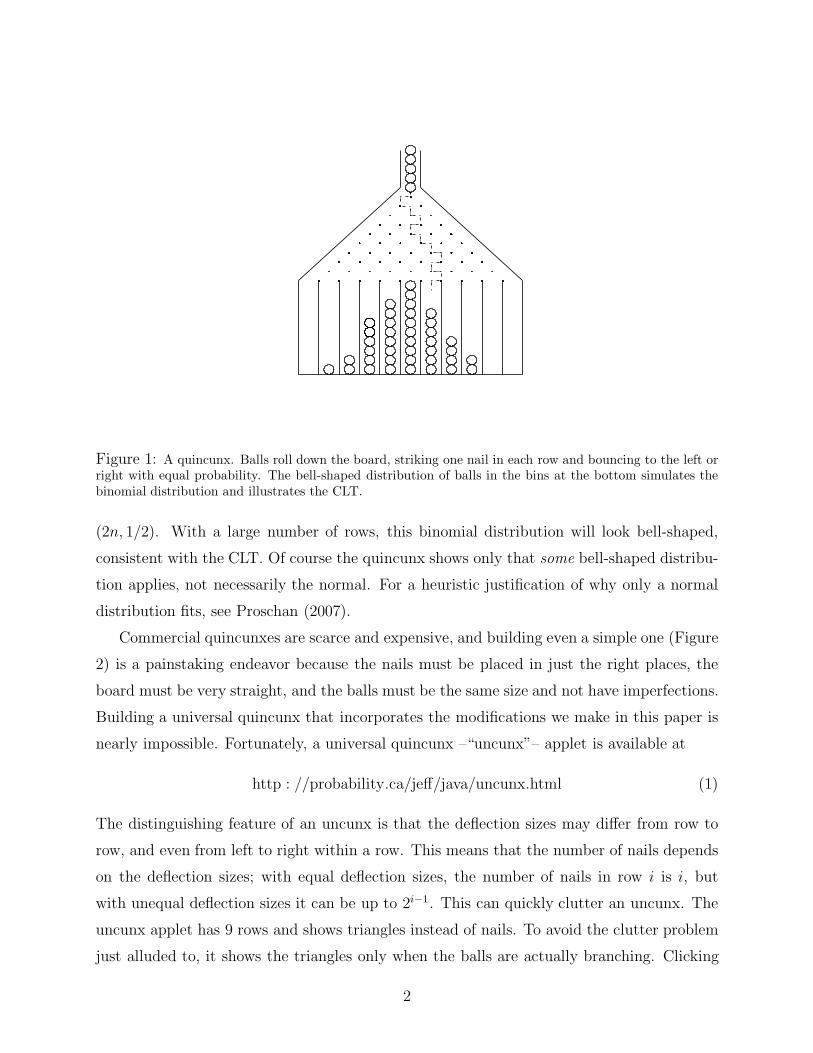
Figure 1: A quincunx. Balls roll down the board, striking one nail in each row and bouncing to the left orright with equal probability. The bell-shaped distribution of balls in the bins at the bottom simulates thebinomial distribution and illustrates the CLT.

(2n, 1/2). With a large number of rows, this binomial distribution will look bell-shaped,

consistent with the CLT. Of course the quincunx shows only that some bell-shaped distribu-

tion applies, not necessarily the normal. For a heuristic justification of why only a normal

distribution fits, see Proschan (2007).

Commercial quincunxes are scarce and expensive, and building even a simple one (Figure

2) is a painstaking endeavor because the nails must be placed in just the right places, the

board must be very straight, and the balls must be the same size and not have imperfections.

Building a universal quincunx that incorporates the modifications we make in this paper is

nearly impossible. Fortunately, a universal quincunx –“uncunx”– applet is available at

http : //probability.ca/jeff/java/uncunx.html (1)

The distinguishing feature of an uncunx is that the deflection sizes may differ from row to

row, and even from left to right within a row. This means that the number of nails depends

on the deflection sizes; with equal deflection sizes, the number of nails in row i is i, but

with unequal deflection sizes it can be up to 2i−1. This can quickly clutter an uncunx. The

uncunx applet has 9 rows and shows triangles instead of nails. To avoid the clutter problem

just alluded to, it shows the triangles only when the balls are actually branching. Clicking

2

on the display and typing “f” or “s” causes the balls to go faster or slower, respectively.

As each ball reaches the bottom of the uncunx, the corresponding histogram bar becomes

taller. Also shown is a normal curve with the same mean and variance as the binomial. As

more balls accumulate, the histogram looks very similar to the normal curve. Later we will

illustrate more sophisticated features of the applet.

Figure 2: A homemade quincunx made with pushpins, rubber bands, a ruler, steel balls, nails, and a board.

This paper argues that the uncunx applet is a wonderful teaching device that can be used

to illustrate many different concepts in probability and statistics, including Pascal’s triangle,

CLTs for independent but not identically distributed random variables, and permutation

tests. The presentation is heuristic rather than rigorous, but the intuition instilled by the

uncunx applet is valuable for statistics students of all levels.

2 Pascal’s Triangle

One reason a quincunx is helpful is that it gets students to think about the number of paths

a ball can take, which can help with combinatorics. For this application only, it is helpful to

number the rows sequentially beginning with 0 instead of the more conventional 1. Similarly,

number the nails in each row sequentially beginning with nail 0. How many paths lead to

nail k of row r of the quincunx? Denote this number by Nr,k. The number of paths is simple

3

Figure 3: The uncunx applet in its default mode with equal row deflections. The superimposed normaldistribution has the same mean and variance as the binomial it simulates.

if k = 0; every deflection must be to the left, so Nr,0 = 1. Similarly, Nr,r = 1. Now consider

nail k of row r, where k 6= 0 and k 6= r. For the ball to strike nail k in row r, in row r − 1 it

must have struck either nail k − 1 and bounced right, or nail k and bounced left. Therefore,

the number of paths leading to nail k in row r is the sum of the numbers of paths striking

nails k − 1 and k of row r − 1. In symbols, Nr,k = Nr−1,k−1 + Nr−1,k (see equation 1.11 on

page 37 of Parzen, 1960). This suggests an iterative way to determine Nr,k. Place a 1 in row

0 and at the extreme left and right ends of each row. To get the number corresponding to

a given nail in a row, add the numbers in the preceding row just to the left and just to the

right of the position in the current row. This is the algorithm for Pascal’s triangle (Table

1). The equation Nr,k = Nr−1,k−1 + Nr−1,k is usually proven by induction, which offers no

intuition. The quincunx is a concrete model that provides the intuition.

3 Central Limit Theorems for Symmetric Binary Ran-

dom Variables

The Introduction explained that the bell-shaped distribution of balls in the different chutes

illustrates the CLT for iid symmetric Bernoulli random variables, but does the CLT hold for

4

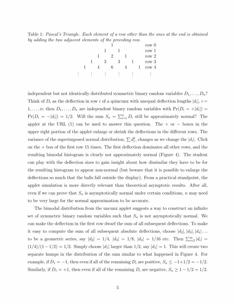
Table 1: Pascal’s Triangle. Each element of a row other than the ones at the end is obtainedby adding the two adjacent elements of the preceding row.

1 row 01 1 row 1

1 2 1 row 21 3 3 1 row 3

1 4 6 4 1 row 4...

......

......

...

independent but not identically distributed symmetric binary random variables D1, . . . ,Dn?

Think of Di as the deflection in row i of a quincunx with unequal deflection lengths |di|, i =

1, . . . , n; then D1, . . . ,Dn are independent binary random variables with Pr(Di = +|di|) =

Pr(Di = −|di|) = 1/2. Will the sum Sn =∑n

i=1 Di still be approximately normal? The

applet at the URL (1) can be used to answer this question. The + or − boxes in the

upper right portion of the applet enlarge or shrink the deflections in the different rows. The

variance of the superimposed normal distribution,∑

d2i , changes as we change the |di|. Click

on the + box of the first row 15 times. The first deflection dominates all other rows, and the

resulting bimodal histogram is clearly not approximately normal (Figure 4). The student

can play with the deflection sizes to gain insight about how dissimilar they have to be for

the resulting histogram to appear non-normal (but beware that it is possible to enlarge the

deflections so much that the balls fall outside the display). From a practical standpoint, the

applet simulation is more directly relevant than theoretical asymptotic results. After all,

even if we can prove that Sn is asymptotically normal under certain conditions, n may need

to be very large for the normal approximation to be accurate.

The bimodal distribution from the uncunx applet suggests a way to construct an infinite

set of symmetric binary random variables such that Sn is not asymptotically normal. We

can make the deflection in the first row dwarf the sum of all subsequent deflections. To make

it easy to compute the sum of all subsequent absolute deflections, choose |d2|, |d3|, |d4| . . .to be a geometric series, say |d2| = 1/4, |d3| = 1/8, |d4| = 1/16 etc. Then

∑∞i=2 |di| =

(1/4)/(1− 1/2) = 1/2. Simply choose |d1| larger than 1/2, say |d1| = 1. This will create two

separate humps in the distribution of the sum similar to what happened in Figure 4. For

example, if D1 = −1, then even if all of the remaining Di are positive, Sn ≤ −1+1/2 = −1/2.

Similarly, if D1 = +1, then even if all of the remaining Di are negative, Sn ≥ 1− 1/2 = 1/2.

5

Figure 4: The applet after clicking on the “+” button in the first row 15 times to make its deflectiondominate all others, causing a bimodal distribution.

Therefore, P (−1/2 < Sn < 1/2) = 0 for all n, and the distribution of Sn has two symmetric

humps. The conditions ensuring asymptotic normality must therefore rule out cases like

this in which one row’s deflection dominates the overall sum. Students in undergraduate

probability and statistics courses need not understand the precise Lindeberg condition that

ensures normality (e.g., see page 239 of Feller, 1957), just that some condition is needed to

prevent one row from dominating.

4 Permutation Tests in A Paired Setting

Sometimes data consist of pairs, one member of which is given a treatment (T) and the other

a control (C). Examples are crossover studies or clinical trials with pair matching. Under

the null hypothesis of no treatment effect, the distribution of paired differences should be

symmetric about 0. One attractive option for analyzing such data is a permutation test

(Good, 2005). We condition on the absolute value of pairwise differences, |di|, i = 1, . . . , n

Conditioned on |di|, the ith paired difference is equally likely to be ±|di|, so the test statistic∑n

i=1 Di is conditionally a sum of independent but not identically distributed binary random

variables. The distribution of this sum is the permutation distribution. The situation is

6

identical to that of the preceding section. We can use the uncunx applet to see whether,

given |d1|, . . . , |dn|, the permutation distribution is approximately normal.

Most statisticians have a vague notion that when the sample size is large, the permutation

distribution is approximately normal, so the permutation test gives the same answer as

the t-test asymptotically. But what does this statement really mean? We saw that it

is possible to make up values |d1|, . . . , |dn| such that the permutation distribution is not

approximately normal, even if n is large. Are such sets of |d1|, . . . , |dn| aberrant, or could they

reasonably arise as iid realizations from a distribution with finite variance? To investigate

this, click on the uncunx display and press “d” for distribution. This causes the applet

to choose row deflection sizes iid from a uniform distribution on [1, 40]. Despite the fact

that this distribution is very spread out and this uncunx has only 9 rows, the permutation

distribution is nearly always approximately normal with mean 0 and variance∑n

i=1 d2i . That

is, Zn = Sn/(∑n

i=1 d2i )

1/2 is approximately standard normal for any values |d1|, . . . , |dn| that

might arise as iid observations from this distribution. More generally, for any distribution

of row deflection sizes with finite variance, the set of infinite realizations |d1|, . . . , |dn|, . . . for

which the permutation distribution of Zn = Sn/(∑n

i=1 d2i )

1/2 does not approach N(0, 1) as

n → ∞ has probability 0 of occurring. In other words, we get the same answer asymptotically

whether we use a t-test or a permutation test in the paired setting. Van der Vaart (1998)

proves the analog of this result in an unpaired setting.

5 The CLT for Symmetric Random Variables

The arguments of the preceding section can be used to deduce that the CLT holds not just for

symmetric binary random variables, but for any iid random variables Di symmetric about 0.

The steps consist of: 1) conditioning on |di|, i = 1, . . . , n, which creates independent, sym-

metric binary random variables; 2) using the uncunx applet to conclude that conditioned on

the |di|, Sn is approximately N(0,∑n

i=1 d2i ), or equivalently, Zn = Sn/(

∑ni=1 d2

i )1/2 is approx-

imately standard normal; 3) arguing that because the conditional distribution of Zn given

|di|, i = 1, . . . , n is approximately standard normal for all possible values |d1|, |d2| . . . , |dn|, . . .(except those in a set of probability 0), Zn is unconditionally asymptotically standard

normal as well; 4) arguing that σ̂2 =∑

D2i /n is very close to E(D2

1) = σ2, so because∑

Di/(∑

D2i )

1/2 = n1/2Sn/σ̂ is approximately standard normal, so is n1/2Sn/σ. From this

argument the student can see that the CLT should hold whenever the iid random variables

7

have a symmetric distribution with mean 0 and finite variance.

6 Random Number Generation

Thus far we have considered random variables symmetric about 0, but an interesting modifi-

cation of the quincunx allows us to visualize the inverse probability transform for generating

random variables with an arbitrary continuous distribution F . In the first row, place the nail

at the median of F . The 2 nails in the second row are placed at the first and third quartiles,

while the 4 nails in the third row are at percentiles corresponding to probabilities 1/8, 3/8,

5/8, and 7/8, and similarly for subsequent rows. When a ball strikes the nail in the first

row, it deflects either to the left or right, striking either the first or second nail in the second

row. The size of the left deflection may not be the same as the size of the right deflection.

Similarly, if the ball deflects left at the first row, hitting the nail at the 1/4 quantile of the

second row, it deflects left or right and strikes either the 1/8 or 3/8 quantile of the third row,

etc. (Figure 5). The distribution of balls at the bottom of this uncunx with a large number

of rows will be arbitrarily close to the density f of F .

Q1 Q2 Q3

Figure 5: Using an uncunx to simulate from an arbitrary distribution. The nail in the first row divides thedistribution into less than or greater than the median. The nail in the second row subdivides into below orabove the quartiles Q1 and Q3. As we add rows, the distribution of balls at the bottom approaches that ofthe continuous curve.

8

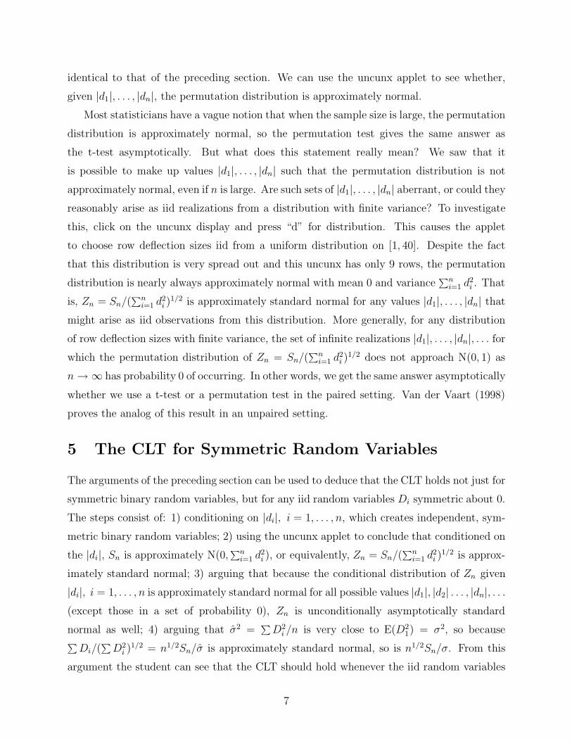
The applet can be used to illustrate this process for four different distributions: gamma

(2, 1), gamma (4, 1), exponential, and lognormal. Click on the display and type “q” for

quantile, which illustrates generation from a gamma (2, 1) distribution (pressing “q” repeat-

edly cycles through the other three distributions and returns to normal mode). The first

row corresponds to the largest deflection because for the gamma (2, 1) distribution the dis-

tance between the median and the first or third quartile is larger than distances between

subsequent quartiles and octiles, etc. The triangles get smaller as we move down the rows.

Because the left-right deflections are of different sizes, the triangles are asymmetric. After

sufficiently many balls have passed through the uncunx, the histogram strongly resembles

the density f(x) (Figure 6).

Figure 6: Using the applet to illustrate simulation from an arbitrary distribution with density f(x) usingthe method described in the legend of Figure 5. The resulting histogram strongly resembles the density f(x).

To see the connection between the applet and the generation of an arbitrary random

deviate from a uniform deviate, imagine placing the nails not at the quantiles of the distri-

bution, but at their corresponding probabilities. That is, the nail in the first row is placed at

horizontal location 1/2, the two nails in the second row are placed at horizontal locations 1/4

and 3/4, etc. Call this the probability uncunx as opposed to the quantile uncunx generated

by the applet in quantile mode. There is exactly one path leading to each of the two nails

in row 2 of the probability uncunx, exactly one path leading to each of the 4 nails in row 3,

9

and more generally, exactly one path leading to each of the 2i−1 nails in row i. Therefore,

the distribution of balls in row i is a discrete uniform on 1, . . . , 2i−1. Take the same set of

left-right deflections generated by the quantile uncunx and superimpose them on the prob-

ability uncunx. As the number of rows increases, the quantile uncunx generates a deviate

from a distribution that is arbitrarily close to F , while the probability uncunx generates a

deviate from a distribution that is arbitrarily close to a uniform [0, 1]. Therefore, there is a

1-1 connection between generating a uniform deviate and generating an arbitrary continu-

ous random variable. The process maps the percentiles of an arbitrary distribution to the

corresponding percentiles of a uniform. The uncunx therefore gives a visual representation

of the well-known result that one can simulate from any continuous distribution function F

by F−1(U), where U is uniformly distributed (see, for example, page 156 of DeGroot, 1986).

The uncunx applet in quantile mode is interesting because the indicators of whether the

deflections are left or right are iid Bernoullis, but the deflection sizes are not independent.

For example, knowing that the first deflection was to the right pins down the deflection size

in the second row to one of two choices; if the first row deflection had instead been to the

left, the deflection size choices in the second row would have been different.

7 Summary

The quincunx allowed early statisticians to perform simulations long before the advent of

modern computers. The problem is that building even a simple physical quincunx is diffi-

cult, and building one that incorporates the modifications in this paper is nearly impossible.

Fortunately, the URL (1) provides a virtual universal quincunx that can be used to demon-

strate a multitude of useful concepts, including the central limit theorem for independent but

not identically distributed random variables, permutation tests in a paired setting, and the

generation of a random variable with an arbitrary continuous distribution from a uniform

variate. Young students are often enthralled by video games, so the uncunx applet may

provide that spark that sways them to go into the field of statistics. Its versatility makes

the uncunx an essential tool in mathematics and statistics classes of all levels.

10

Acknowledgment

We would like to thank the referees, editor, and associate editor for suggestions that improved

the paper markedly, and Wendy Lou, who introduced us to each other.

References

1. DeGroot, M.H. (1986). Probability and Statistics, 2nd ed. Addison Wesley, Reading

Massachusetts.

2. Feller, W. (1957). An Introduction to Probability Theory and Its Applications, Vol 1.

John Wiley and Sons, New York.

3. Good, P. (2005). Permutation, Parametric, and Bootstrap Tests of Hypotheses, 3rd ed.

Springer, New York.

4. Kunert, J., Montag, A., and Pohlmann, S. (2001). The quincunx: history and mathe-

matics. Statistical Papers 42, 143-169.

5. Parzen, E. (1960). Modern Probability Theory and Its Applications. John Wiley and

Sons, New York.

6. Proschan, M.A. (2008). The normal approximation to the binomial. The American

Statistician 62, 62-63.

7. Stigler, S.M. (1986). The History of Statistics: The Measurement of Uncertainty before

1900. The Belknap Press of Harvard University Press. Cambridge, Massachusetts.

8. van der Vaart, A.W. (1998). Asymptotic Statistics. Cambridge University Press.

11